
Four-Dimensional Plant Phenotyping Model Integrating Low-Density LiDAR Data and Multispectral Images


School of Engineering, Pontificia Universidad Javeriana Bogota, Cra. 7 No. 40-62, Bogotá 110231, Colombia
*
Author to whom correspondence should be addressed.
Remote Sens. 2022, 14(2), 356; https://doi.org/10.3390/rs14020356
Submission received: 29 November 2021
/
Revised: 16 December 2021
/
Accepted: 21 December 2021
/
Published: 13 January 2022
(This article belongs to the Special Issue 3D Modelling and Mapping for Precision Agriculture)
Abstract
:High-throughput platforms for plant phenotyping usually demand expensive high-density LiDAR devices with computational intense methods for characterizing several morphological variables. In fact, most platforms require offline processing to achieve a comprehensive plant architecture model. In this paper, we propose a low-cost plant phenotyping system based on the sensory fusion of low-density LiDAR data with multispectral imagery. Our contribution is twofold: (i) an integrated phenotyping platform with embedded processing methods capable of providing real-time morphological data, and (ii) a multi-sensor fusion algorithm that precisely match the 3D LiDAR point-cloud data with the corresponding multispectral information, aiming for the consolidation of four-dimensional plant models. We conducted extensive experimental tests over two plants with different morphological structures, demonstrating the potential of the proposed solution for enabling real-time plant architecture modeling in the field, based on low-density LiDARs.
1. Introduction
Global agriculture faces major challenges to ensure the world’s food security, specially because the annual increase in crops yield achieved by traditional breeding methods around the world are no longer sufficient to meet the projected demand. In that context, one particular challenge is the need to produce high-yielding crops adapted to future climate changes and resilient to several biotic factors and abiotic stresses (Furbank et al. [1]).
Crop phenotyping offers a set of new technologies to understand the traits resulting from the interaction of genes and the environmental conditions that surround crops, thus allowing actions to improve crop performance (Furbank et al. [2], Reynolds et al. [3] and Tester et al. [4]). In plants, phenotyping specifically refers to a quantitative description of the morphological, physiological and biochemical parameters of plants. In order to obtain these parameters, traditional methods involve manual and direct manipulation of the plants, leading to a destructive process (Paulus et al. [5], Furbank et al. [1] and McCouch. [6]). However, with the recent advances in the field and the use of new technological tools, such as 3-dimensional (3D) reconstruction and analysis of conventional and multispectral images, these parameters can be estimated without affecting the integrity of the plants (Mokarram et al. [7]).
As the physiological and biochemical parameters of plants (vegetative indices) are three-dimensionally distributed, the multispectral images that can be acquired should also be mapped to the morphological parameters of the plant, which is commonly referred to as four-dimensional (4D) phenotyping models (Apelt et al. [8]). Plant model phenotyping approaches have recently gained significant traction to characterize functional-structural plant traits, in order to associate the phenotypic data with genomic information. Most of the body of work relies on optical techniques such as photoluminescence and photoacoustics for both inorganic and organic compounds detection. However, imaging-based plant phenotyping has demonstrated to be more portable, with the advantage of producing 4D models of plants that would significantly aid phenotyping practice and increase accuracy and repeatability of the measurements of interest (Donald et al. [9]). Nonetheless, a single optical sensor is not capable of producing a comprehensive 4D plant model, since the morphological information of the plant must be also fused with multispectral data and the time evolution of the interested variables of the plant, such as leaf nitrogen and chlorophyll, vegetation indices, among others. In this regard, 4D plant architecture refers to computational models that combine: (i) 3D plant geometrical information (point cloud data), (ii) several wavelengths of light reflectances (multi-spectral imagery), and (iii) the temporal evolution of the phenotyping variables. Based on that, multisensor platforms are necessary to achieve an effective combination of the spatial, geometric, and temporal components of the multiple streams of information coming from different sensors, for instance, multispectral cameras and LiDARs. which is commonly referred as sensory fusion (Luo et al. [10])
Sensory fusion between 3D and 2D time-of-flight (ToF) sensors has already been used in plant phenotyping, using different methods to accomplish this task. For instance, in (Hosoi et al. [11]) perspective projections with multispectral images acquired with the Micasense camera and dense point clouds (with an error range of up to 2 mm) from the Focus 3D X330 LiDAR were used to find the chlorophyll distribution in Yoshino cherry and bamboo-leaved oak trees.
In [12], Sun et al. used RGB-D (RGB and depth) images from a Kinect camera and images from the SOC710 hyperspectral camera to perform sensory fusion between these two sensors and obtain distributed biochemical parameters of plants. For the fusion of information between these two sensors, the authors first performed a registration between the RGB-D images and the hyperspectral images, according to the principles of the Fourier transform, calculating the translation, the rotation matrix and the scale coefficients of the images to be registered. Once the registration between the images was done, they generated a 3D point cloud from the RGB-D image with the multispectral information, and by measuring the plant in steps of (4 takes in total) and registering these four point clouds, they obtained a distributed reconstruction of the biochemical parameters of the plants.
In [13], Itakura et al. took 50 sample images (utilizing a Canon EOS M2 camera) of an eggplant plant and using the structure-from-motion (SfM) methodology (Haming et al. [14]) they obtained a 3D representation of the plant. Then, taking the normalized red channel of the 3D object, they estimated the chlorophyll levels of the plant. In a related work, in [15] Zhang et al. used a SLR camera with near-infrared filters on the lens to estimate vegetative indices and chlorophyll level of rice plants. Then, using the multiview passive 3D reconstruction method (El Hazzat et al. [16]), they created 3D reconstructions of the plant with its vegetative indices and chlorophyll-level information.
Phenotyping platforms offer a powerful alternative to traditional methods for understanding plant behavior. These platforms provide non-destructive and unbiased methods to quantify complex and previously unattainable plant traits (Perez-Ruiz et al. [17]). At plant scale, there are studies on 4D phenotyping platforms, however, these studies use 2D sensors or structured light methods to reconstruct the plant in 3D, but do not use 3D sensors such as LiDAR radars or 3D scanners. In fact, although there are studies that integrate the use of LiDAR radars for the extraction of plant morphological parameters (Jimenez-Berni et al. [18], Hosoi et al. [11] and Thapa et al. [19]), these studies do not consider a sensory fusion to extend the plant’s physiological and biochemical parameters into a 3D space, which in most of the cases, are paramount for predicting and estimating plant and crop yields (Reynolds et al. [3]). Most of these approaches require bulky equipment that would not allow the on-site extraction of these parameters.
Considering this, we proposed the development of a flexible and portable phenotyping platform, fusing low-density LiDAR data and multispectral imagery to generate four-dimensional plant models. With that purpose, we utilize the Velodyne’s VLP-16 LiDAR and the Parrot’s Sequoia multispectral camera, and by integrating a novel set of mechanisms that also involves the calibration of the intrinsic and extrinsic parameters of these sensors, we are capable of implementing a sensory fusion that allows us to generate 4D phenotyping models where morphological and biochemical parameters of plants can be estimated.
2. Materials and Methods
This section will present the materials and equipment utilized, as well as the algorithms and methods proposed and implemented for this work.
2.1. Materials
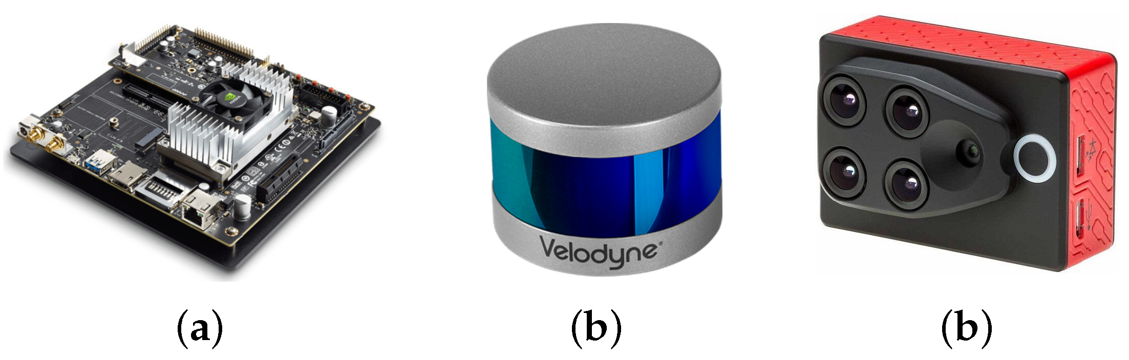
As it was mentioned before, one of the goals of the project is to have a flexible and portable platform, which requires the utilization of an embedded device to perform the control of the sensors and the corresponding processing and generation of the 4D phenotyping model. The embedded system that we used for this project was NVIDIA’s Jetson TX2 (see Figure 1a) that integrates NVIDIA’s Denver2 dual-core, an ARM Cortex-A57 quad-core, 8 GB 128 bit LPDDR4 RAM and a 256-core Pascal GPU which becomes very useful for implementing machine vision and deep learning algorithms. The Jetson TX2 runs Linux and provides more than 1TFLOPS of FP16 compute performance in less than 7.5 W of power.
As presented before, we integrated Velodyne’s VLP-16 LiDAR (see Figure 1b) which has a range of 100 m, low power consumption (aprox. 8 W), a weight of 830 g and a compact form factor (⌀103 mm × 72 mm). This LiDAR also supports 16 channels (approx. 300,000 points/s), a horizontal field of view of and a vertical field of view of . Since this specific LiDAR has no external rotating parts, it is highly resistant in challenging environments (IP67 rating). For each sensed point, this sensor generates: (i) position , (ii) intensity of the received signal, (iii) azimuth angle with which the point was sensed, and (iv) ID of the laser beam that acquired the point.
In order to control and capture the information that the LiDAR sensor, we developed a Python library that allows the connection to the sensor through an Ethernet interface, its setup (e.g., selecting the number of samples to be sensed) and performs the preprocessing necessary to store the corresponding point clouds.
In addition to the LiDAR, we included the Parrot’s Sequoia multispectral camera (see Figure 1c), which in addition to images in the visible spectrum (RGB), it also captures the calibrated wavelength green (GRE), red (RED), red-edge (REG), and near-infrared (NIR), providing rich data to properly monitor the health and vigor of crops and plants. The Sequoia camera generates a WiFi access point, through which it is possible to control and access the information of the camera. With this purpose, another Python library was developed which allows us to connect to the Sequoia camera and, through HTTP requests, to access and control the multispectral imaging.
In order to properly acquired a model of the plan, a mechanical structure was designed and constructed entirely of modular aluminum to ensure that it can be disassembled and easily transported. In addition, the structure has a rail system that allows the sensors (multispectral camera and LiDAR) to move vertically on a 1.8 m aluminum profile and to move the rotating base closer or farther from the sensors on a 2 m aluminum profile. Additionally, it has leveling screws on the four legs of the platform, in order to adjust the inclination of the mechanical structure. In comparison with the structures in other investigations (Thapa et al. [19], Sun et al. [12,20], Zhang et al. [15]), the proposed structure (shown in Figure 2) is able to freely move both the sensors and the rotating base over the rails system allowing the phenotyping of plants with a height up to 2.5 m, regardless of their structure.
The implemented rotating base is controlled by the Jetson TX2 embedded platform and it uses a Nema 700 motor and a crown/gear system. To control the positioning of the rotating base, the Ky-040 rotary encoder was used, achieving steps down to .
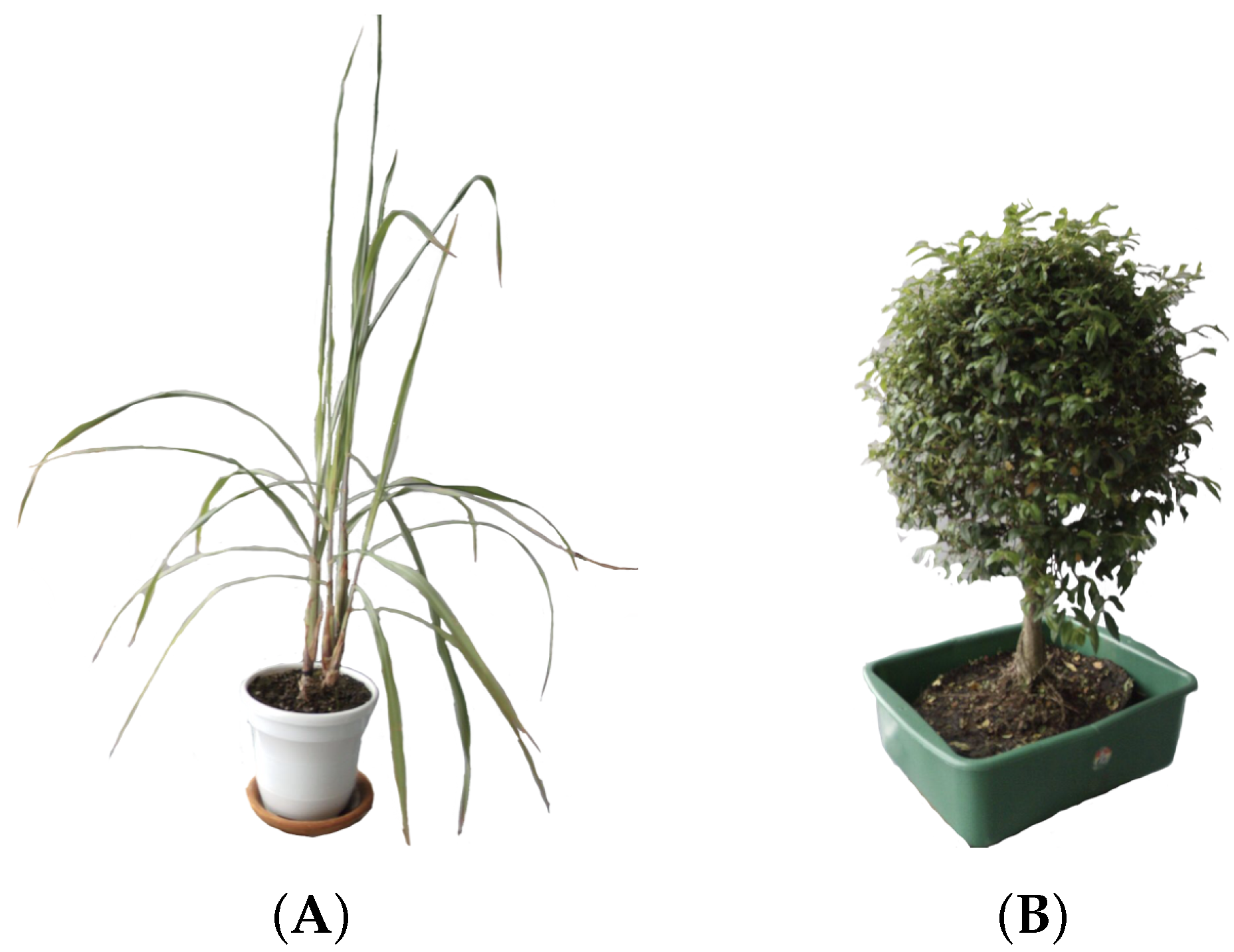
Due to the difficulty to properly maintain a rice plant into a laboratory environment, we selected one plant with a structure similar. The plant chosen was Limonaria (Cymbopogon citratus), which belongs to the grass family, Poaceae. Its leaves are simple, green, with entire margins and linear shape. The leaves are usually 20–90 cm long and, like other grasses, the leaves also have parallel venation. The particular Limonaria used during the experimentation stages had a height of 97 cm from the base of the stem to the tip of its highest leaf (see Figure 3A).
Since we wanted to properly characterize the resulting systems, another plant with a completely different structure was also utilized. The Guaiacum bonsai (cuaiacum officinale) has a bush-like structure that allowed us to qualitative measure the accuracy of the generated model. The Guaiacum used in the experimentation stages had a height of 67 cm from the base to the tip of its canopy (see Figure 3B).
2.2. Methods
A general architecture of the proposed system is shown in Figure 4. Our approach to obtaining 4D phenotyping models is based on four main components: (i) the estimation of vegetative indices, (ii) the generation of a filtered point cloud, (iii) the sensory fusion process based on the calibration of the intrinsic and extrinsic parameters of the sensors, and (vi) a point cloud registration process.
2.3. Extraction of Vegetative Indices
To obtain correct vegetative indexes, it is necessary to register the bands coming from the multispectral camera, otherwise, when performing the operations between the multispectral bands, the resulting image of the vegetative index will be misaligned. The process of registering the images consists of taking different images and finding key points in common between them. Then, selecting a reference image and using the key points found to obtain a homography matrix for each remaining image, which allows to apply geometric transformations to the images and thus register them to the reference image.
With the homography matrices of each multispectral image and using Equations (1)–(6), the vegetative indices are estimated. The process of estimating vegetative indices with multispectral images is presented in Algorithm 1.
| Algorithm 1: Algorithm for estimating vegetative indices with multispectral imagery. |
 |
2.4. Point Cloud Processing
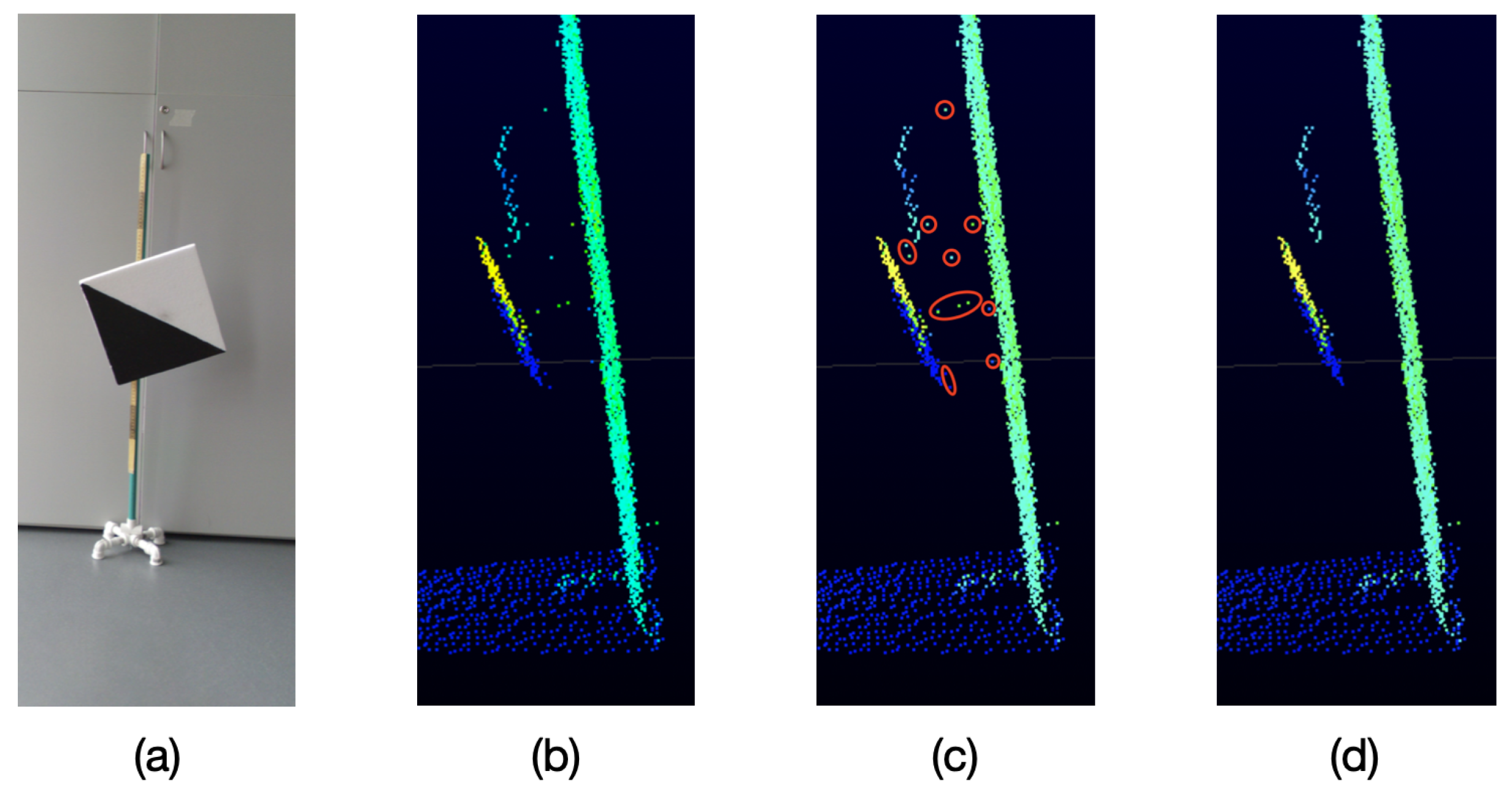
As it can be seen in Figure 5, because of the particular characteristics of the VLP-16 LiDAR, when an object is sensed and behind it there is another object at a distance of approximately 40 cm or less, unwanted points are generated in the space between both objects,
These unwanted points appear near the edges of the sensed object which is closest to the LiDAR. This effect occurs when a laser beam hits the edge of the closest object as well as the object behind it, as represented in Figure 6. Therefore, the LiDAR receives the two measurements and delivers an average of these, which becomes the unwanted point.
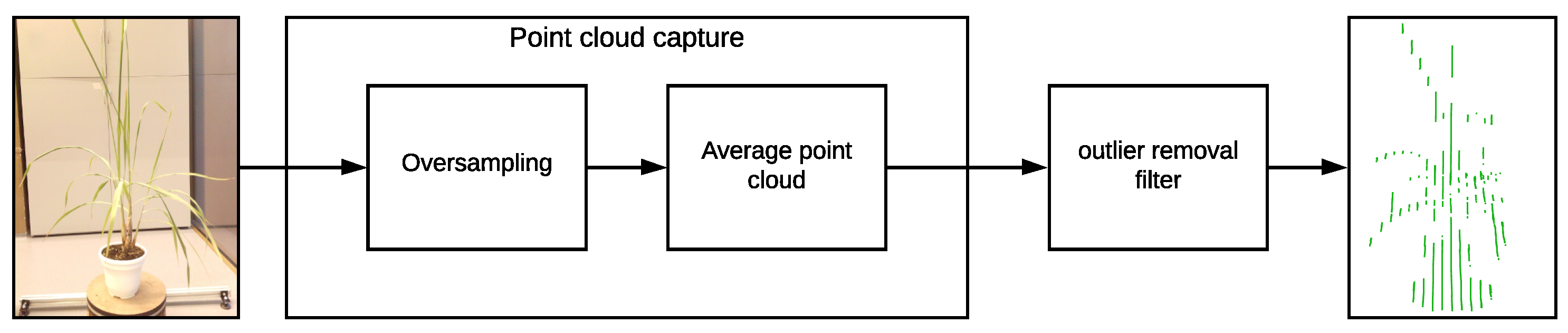
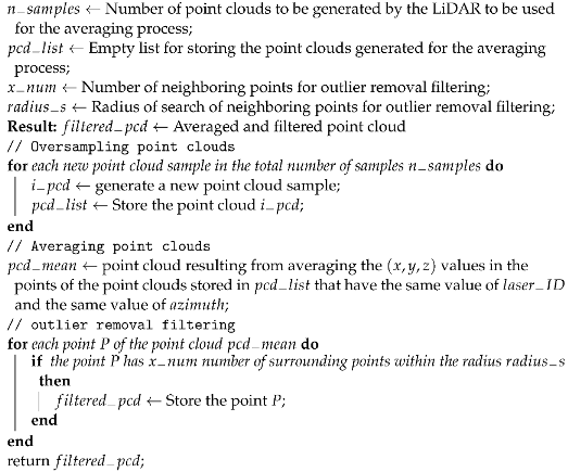
In order to solve this issue and considering that the VLP-16 LiDAR has an accuracy of ±3 cm and a low vertical resolution, a process of oversampling, averaging, and filtering is performed on the point clouds to improve the accuracy of the acquired data and for removing outliers. This oversampling, averaging, and filtering process is described in Figure 7 and in Algorithm 2.
For the oversampling and averaging process, different samples of the plant were acquired, and in order to obtain a single point cloud an averaging process is performed. The points with the same were combined by averaging the values, as well as their values.
For the outlier removal filtering process, a number of neighboring points and a search radius are defined. We expect that each point in the cloud has a typical number of neighboring points, based on the LiDAR resolution. Points in the cloud that do not meet this typical number are considered outliers and hence are removed from the point cloud.
| Algorithm 2: Algorithm for averaging and outlier removal filtering VLP-16 LiDAR point clouds. |
 |
2.5. Sensory Fusion: 3D and 2D Calibration
In order to generate 3D models that includes color information, different algorithms have been proposed that seek sensory fusion between LiDAR point clouds and imagery.
Park et al. [21], Debattisti et al. [22], Hurtado et al. [23], Li et al. [24] and Zhou, Deng. [25]) have utilized sensorial fusion of LiDAR radars and conventional cameras, in order to generate point clouds with color information that represent 3D objects. To carry out this fusion, different calibration methods were considered, including linear regressions, random sample consensus algorithms (RANSAC), among others.
For instance, Park et al. [21] and Debattisti et al. [22] used a unicolor diamond-shaped and triangle-shaped boards to find the corresponding points (vertices of the boards) between the LiDAR point clouds and RGB images. With a simple linear regression, it was possible to find the calibration matrix that allowed the fusion between the sensors.
De Silva et al. [26] proposed a calibration board with a circular shape, where the center of the circle was used as the point of correspondence between the point clouds and the RGB images. In a similar approach, Rodriguez et al. [27] found the calibration matrix to align and fuse the information between the sensors, by applying absolute orientation photogrammetry.
In our approach to implement a fusion between the LiDAR data (3D) and the multispectral images (2D), an intrinsic and extrinsic parameter calibration method is required, which is composed of three main stages: (i) the detection of key points in the images (2D) by using a half colored diamond-shaped calibration board; (ii) the detection of key points in the point cloud (3D) by using a diamond-shaped calibration board; and (iii) the application of the random sample consensus (RANSAC) algorithm to find the projection matrix that allows the alignment of the sensor data.
2.5.1. Calibration Board
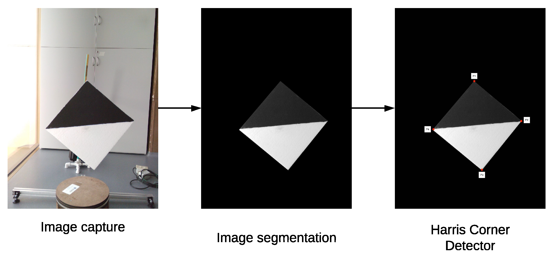
In order to automate the calibration process, we proposed a diamond-shaped calibration board with one half painted black and the other half painted white, as seen in Figure 8. The calibration board has this shape because its vertices can be easily located using the data acquired by the LiDAR, even if it has a low vertical resolution. In addition, in the case of 2D images, there is already a large number of algorithms oriented to find vertices within images.
Since the signal intensity measured by the LiDAR in each 3D point varies according to the material and color of the surface where the LiDAR’s lasers bounce, the selected colors for the calibration board are white and black. When the lasers bounce off on a white colored surface, the LiDAR receives signals with a higher intensity, when compared to the case of a black surface. This difference in intensity levels at the 3D points can later be used to verify the calibration between the LiDAR and the multispectral camera.
2.5.2. Key Points Extraction
To find the key points in the 2D images, a background subtraction in order to isolate the calibration board and, then, a morphological opening transformation is applied to filter the pixels that do not belong to the calibration board. Afterwards, the resulting image is converted to grayscale and a Harris corner detector is applied to find the key points (Ardeshir et al. [28]). This process is described in detail in Algorithm 3.
| Algorithm 3: Algorithm to obtain the key points of a 2D image. |
| Background image (without calibration board); Image with calibration board; Empty list for storing the key points of the image; Result: key points of the image (corners of the calibration board) Image resulting from a background subtraction between the images and ; Image resulting from applying the opening transformation to the image ; in grayscale; Key points found by a corner detector on the image ; return |
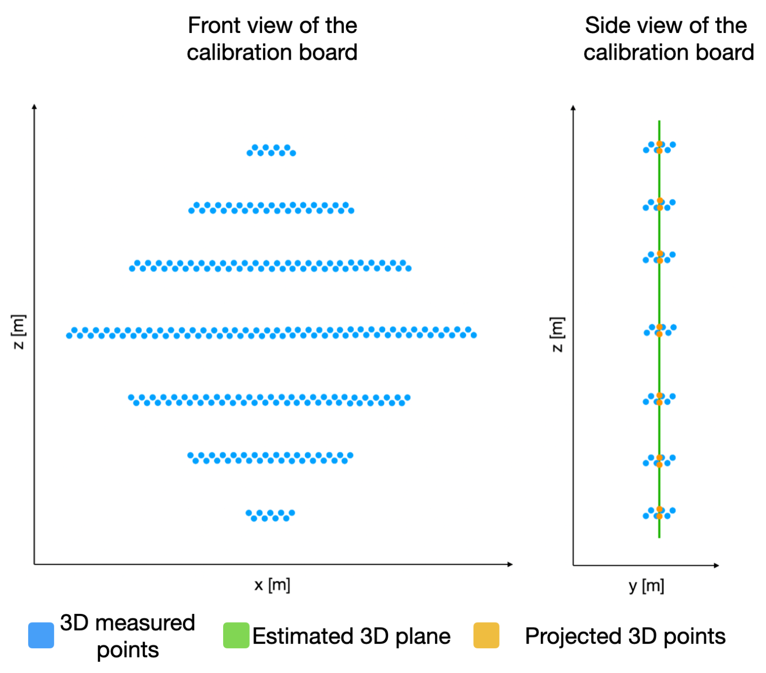
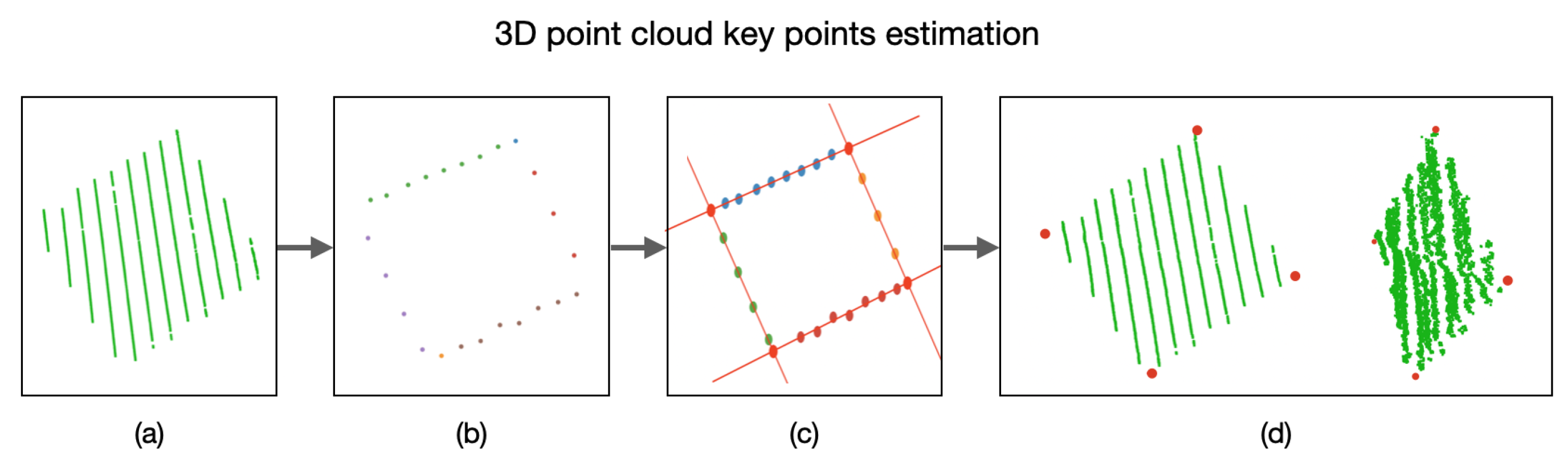
In order to identify the key points in the 3D point cloud, we must first estimate a plane P that satisfies as many 3D points (belonging to the calibration board) as possible, as presented in Figure 9. This plane P is built using the depth information of each 3D point with respect to its coordinate. With this goal in mind, the RANSAC algorithm is applied on the acquired 3D points that belong to the calibration board.
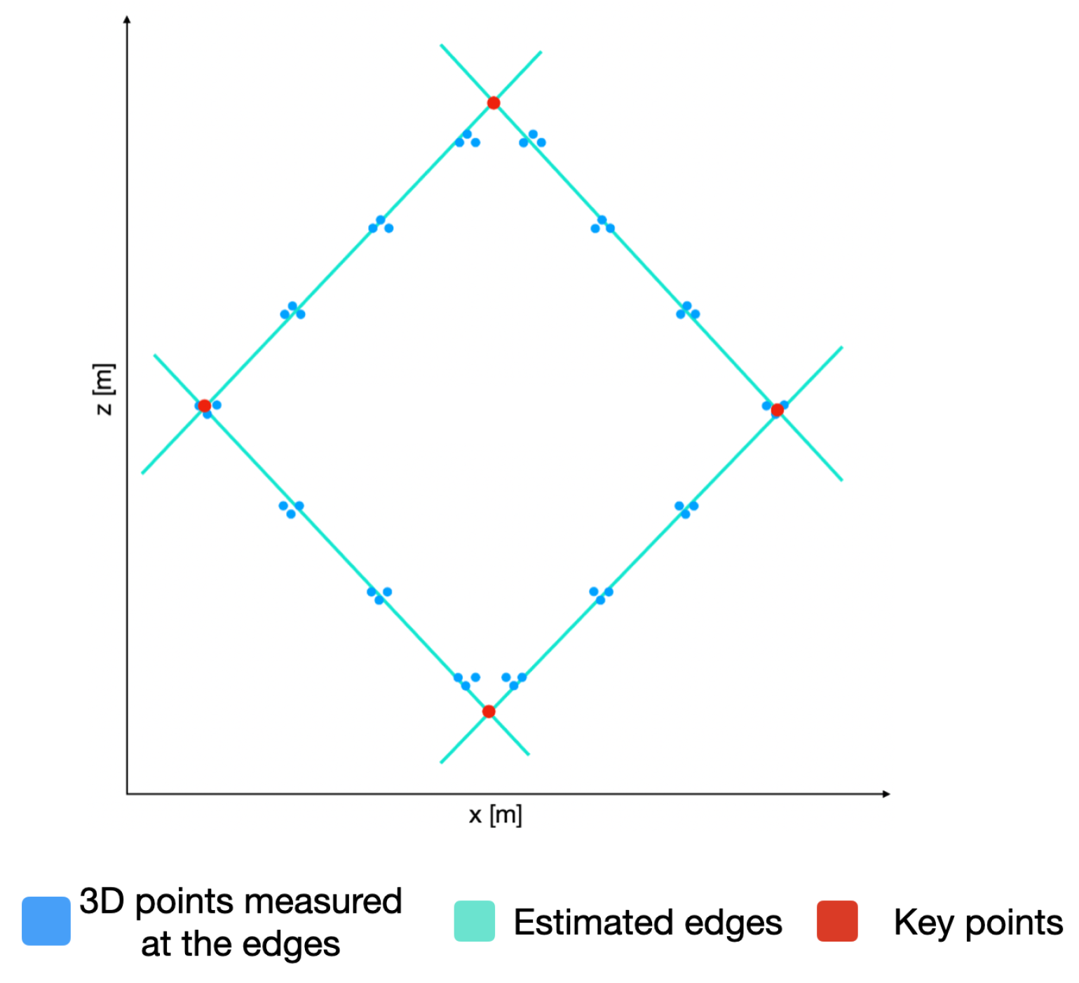
With the plane P and using only the coordinates of the 3D points, we can now detect the edges of the calibration board and, hence, the lines describing these edges. In order to do so, the RANSAC algorithm is used again to estimate the lines describing the edges. By equating these lines, the coordinates of the key points of the calibration board are estimated, as presented in Figure 10. By utilizing the plane P, we can obtain the 3D coordinate of the detected key points.
2.5.3. Sensory Fusion between Point Clouds and Images
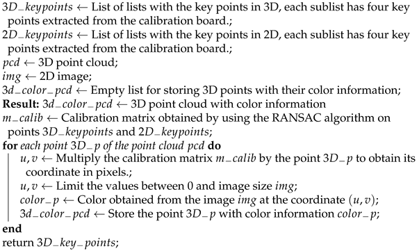
Considering the widely known pinhole camera model (Ardeshir et al. [28]), it is possible to build matrices that relate the intrinsic and extrinsic parameters of a camera and a LiDAR, as presented in Equation (7). Through this relationship between the parameters of the sensors, it is possible to create a projection of the 3D points to the 2D space in order to estimate the fusion of the information.
where are the pixel coordinates of the projection of point A; are the spatial coordinates of point A; and are the effective focal distances; is the center point of the image plane; and R and t are the rotation and translation matrices of the image. These matrices can be represented as a projection matrix C that transforms the coordinates from 3D space to 2D space.
As shown in Equation (8), to solve the projection matrix C at least 12 corresponding points must be found between the 3D and 2D spaces, and using the RANSAC algorithm to find the values that represent the variables of the projection matrix.
Once the projection matrix C is obtained, each 3D point can be projected onto a 2D image and the corresponding color for that point in 3D space can be obtained. Algorithm 4 presents the steps to perform the sensory fusion between point clouds and images.
| Algorithm 4: Algorithm to perform sensory fusion between point clouds and images. |
 |
For the verification of the calibration method, we propose an algorithm that first applies a thresholding stage to the laser intensity for each point in space in order to classify them as black or white 3D points, and also a thresholding stage to the fused color values in order to classify them as black or white color points. With this information, we compare each 3D point with its corresponding fused color point, in order to verify if they are both classify as black or white. Then, by calculating the ratio between the erroneous points and the total number of points in the point cloud, an error measurement of the sensory fusion is estimated.
2.6. Point Cloud Registration for a 360 Model
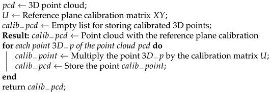
To obtain the 360 model of the plant, it is necessary to perform a calibration of the point clouds to adjust them to the reference plane of the sensors. Subsequently, because the plant is rotating and the sensors are fixed while it is being sensed, a rotation and translation of the point clouds must be performed with reference to the angle at which the rotating base was located when the plant was sensed.
Since the rotating base may have an inclination and it could not be completely parallel to the ground or to the reference plane of the sensors, it is necessary to perform a calibration that allows to correct such inclination. In this way, we are able to make a correct registration of the sensed point clouds at different angles of the rotating base. To perform such plane calibration, it is necessary to find a transformation matrix U that aligns the rotating base plane described in Equation (9), to the reference plane of the sensors described in Equation (11).
With Equation (9), we can find the unit vector A that is normal to the plane, as presented in Equation (10).
The reference plane of the sensors can be considered without inclinations and represented by Equation (11).
With Equation (11) of the plane of reference of the sensors, the unit vector B that is normal to the plane can also be found, as presented in Equation (12).
With the two unit column vectors, A and B and . It is worth noticing that the rotation from A to B is only a 2D rotation on a plane with the normal . This 2D rotation by an angle is given by Equation (13).
However, since A and B are unit vectors, it is not necessary to compute the trigonometric functions since and , and then the rotation matrix can be described by Equation (14).
This matrix represents the rotation of A towards B in the base consisting of the column vectors in Equations (15) (normalized vector projection of A onto B), (16) (normalized vector projection of B on A) and (17) (cross product between B and A). All these vectors are orthogonal and form an orthogonal basis.
The corresponding basis change matrix is represented by Equation (18).
Therefore, in the original basis, the rotation from A to B can be expressed as the right multiplication of a vector by the matrix in Equation (19), arriving at Equation (20).
Therefore, to calibrate the reference plane of the measurements, it is necessary to multiply each point in the point cloud by matrix U. Algorithm 5 presents the general steps to calibrate the sensed reference plane.
| Algorithm 5: Algorithm for calibrating the reference plane of point clouds. |
 |
2.6.1. Calibration of the Rotating Base’s Center
The LiDAR delivers the distance information of a point in the axes regarding to its own center, as it can be seen in Figure 11. Hence, in order to rotate the point clouds relative to the angle of the rotating base, it is necessary to find the coordinates of the center of the rotating base.
In order to find the axis of rotation of the rotating base, a guide object is placed in the center of the rotating base. Then, using the rails of the structure shown in Figure 12, the sensors are moved until one of the LiDAR’s lasers detects the guide object. Once this happens, the position of the center axis of the rotating base is estimated, following Algorithm 6.
| Algorithm 6: Estimation of the coordinates of the axis of rotation of the rotating base. |
| ← point cloud with the calibration of the reference plane belonging to the rotating base and to the guiding object; Result: rotating axis’ coordinates of the rotating base ← laser ID to which the points with the highest values belong to the axis Z; ← points coming from the laser(); ← coordinate of the maximum value on the Y-axis of the points of the ; ← points with coordinates located within a radius of around the coordinate ; average coordinates’ value of the points of ; return |
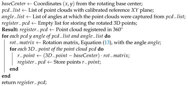
2.6.2. Point Cloud Rotation
To register the point clouds, first, a translation from the acquired point clouds to the origin point of the LiDAR’s coordinate system must be performed. To perform this translation, it is necessary to subtract each point from the point cloud with the center of rotation’s coordinates of the rotating base. Once the point clouds have been translated, each one must be rotated by a rotation angle that is given by the angle at which the rotating base was at the time of capturing the point cloud.
After the plane calibration, the point clouds’ rotation could be expressed by the rotation matrix described in Equation (13). This translation and rotation process is presented in Algorithm 7.
| Algorithm 7: Rotation of point clouds for the 360 registration |
 |
3. Results
3.1. Extraction of Vegetative Indexes
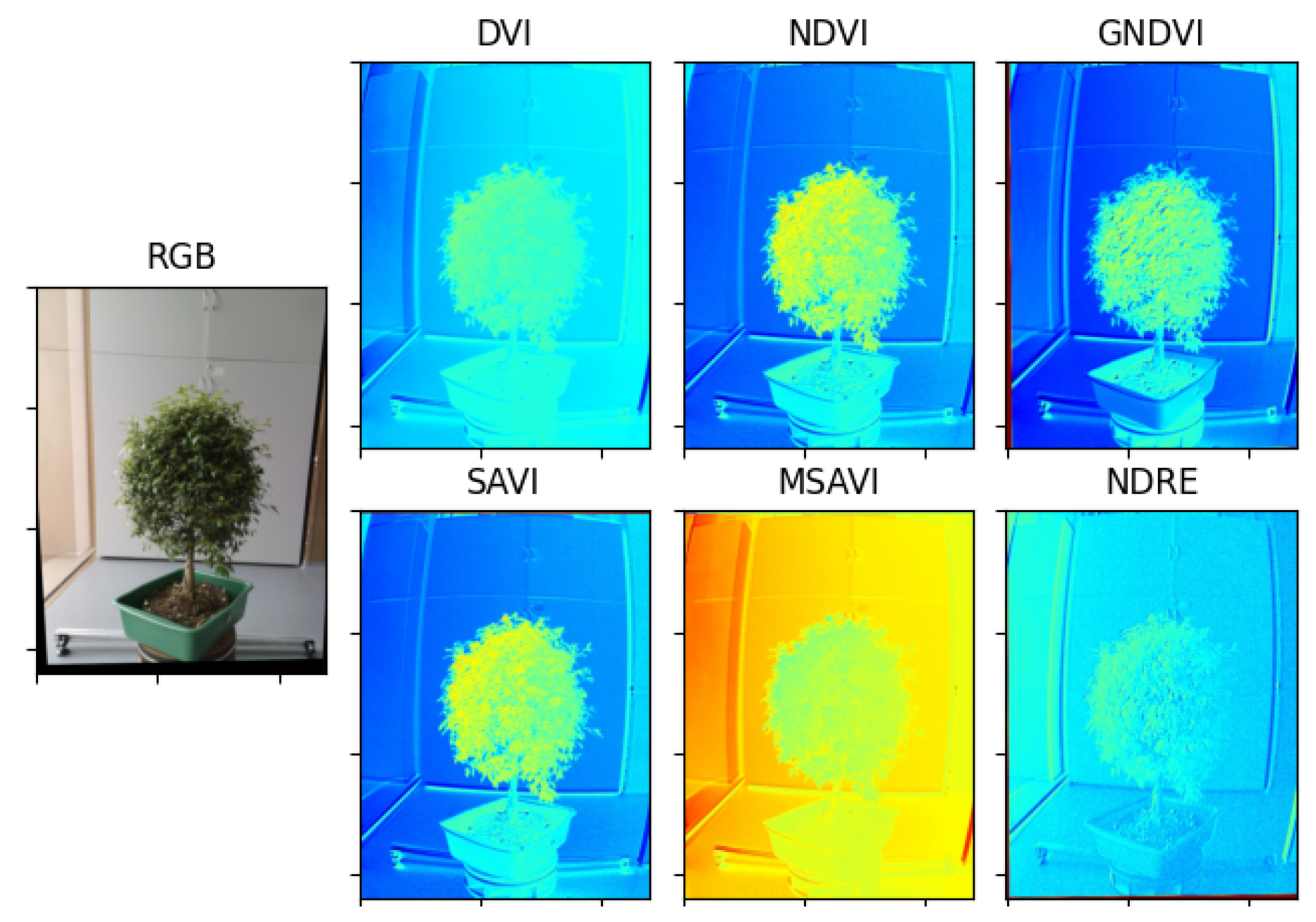
Multispectral photographs were taken to the Limonaria and Guaiacum plants in order to estimate their vegetative indices. Subsequently, using the images from the NIR, REG, RED, and GREEN multispectral bands already registered to the NIR band, the vegetative indices, DVI, NDVI, GNDVI, NDRE, SAVI, and MSAVI, of the plants were calculated. Figure 12 and Figure 13 present the results obtained for each of the vegetative indexes.
Vegetation indices are widely used to quantify plant variables by associating certain spectral reflectances that are highly related to variations in leaf chemical components such as nitrogen, chlorophyll, and other nutrients. In this regard, vegetation indices are key features to characterize the health status of a plant. From the extensive list of vegetation indices available in the specialized literature [29,30,31], we selected 6 vegetation indices with sufficient experimental evidence and quantitative trait loci (QTL)-based characterization regarding their high correlation with plant health, specifically, the photosynthetic activity associated with certain spectral reflectances: green and near-infrared bands.
The Parrot Sequoia multispectral camera comes with a radiometric calibration target that enables reflectance calibration across the spectrum of light captured by the camera. Additionally, the camera has an integrated irradiance sensor designed to correct images for illumination differences in real time, enabling precise radiometrically response, with narrow discrete Red, Green, Red-Edge, and Near-Infrared bands. Regarding the lens disparity, we have observed minimum and neglectable misalignments of pixels between the spectral bands [9], which do not require further image processing for co-registration.
3.2. Oversampling and Point Cloud Processing
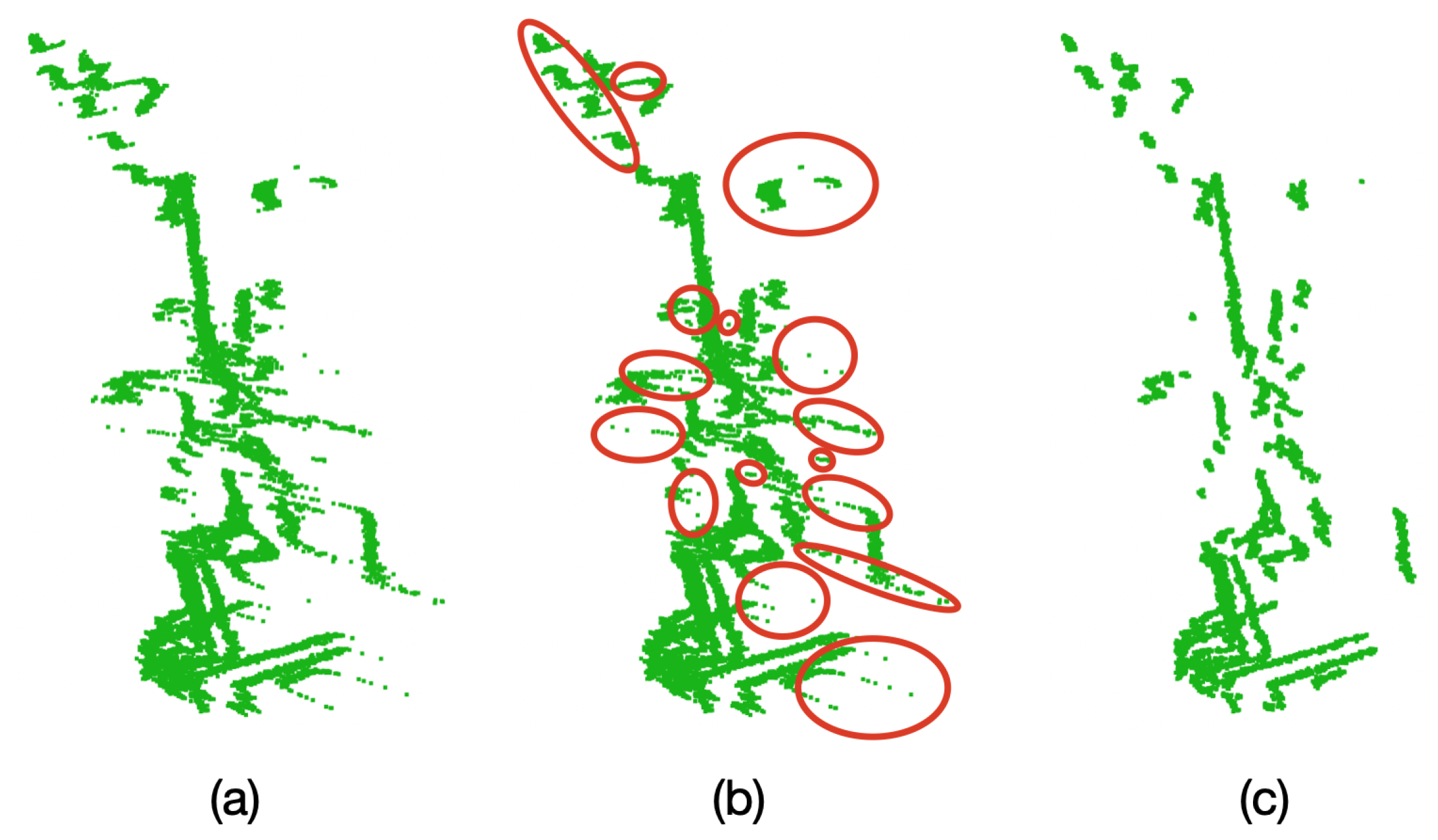
Due to the characteristics of the VLP-16 LiDAR, during the scanning of an object (a plant in this case) if there is another object behind it at a distance of approximately 40 cm or less, unwanted points are generated in the space between the objects. This behavior negatively affects the model generation of plants with long leaf architectures, as these unwanted points will be considered as part of the leaves. To eliminate these unwanted points, the oversampling and filtering of the point clouds described in Algorithm 2 was implemented and tested with the Limonaria plant.
In order to carry out this test, 10 complete samples (1 sample = 1 point cloud) were taken before any rotation is performed on the plant. With these samples, the average point cloud was found and the outlier filter described in Algorithm 2 was applied. Figure 14 presents the results of this test.
3.3. Sensory Fusion: 3D and 2D Calibration
To find the key points in the 2D image, 16 images of the calibration board were captured at different positions. After applying Algorithm 3, 64 key points were found within these images, as presented in Figure 15.
Afterwards, in order to find the key points in the 3D point cloud, 16 point clouds were taken from the calibration board at different positions. By applying the mechanisms detailed before, 64 key points were found within the point clouds, as presented in Figure 16.
With the 64 key points found in the 2D images and the 64 points found in the 3D point clouds, the Algorithm 4 was used to find the calibration matrix that allows the sensory fusion between sensors. Subsequently, to verify the result of this sensor calibration, five new 2D images and five point clouds were acquired with the calibration board at different positions.
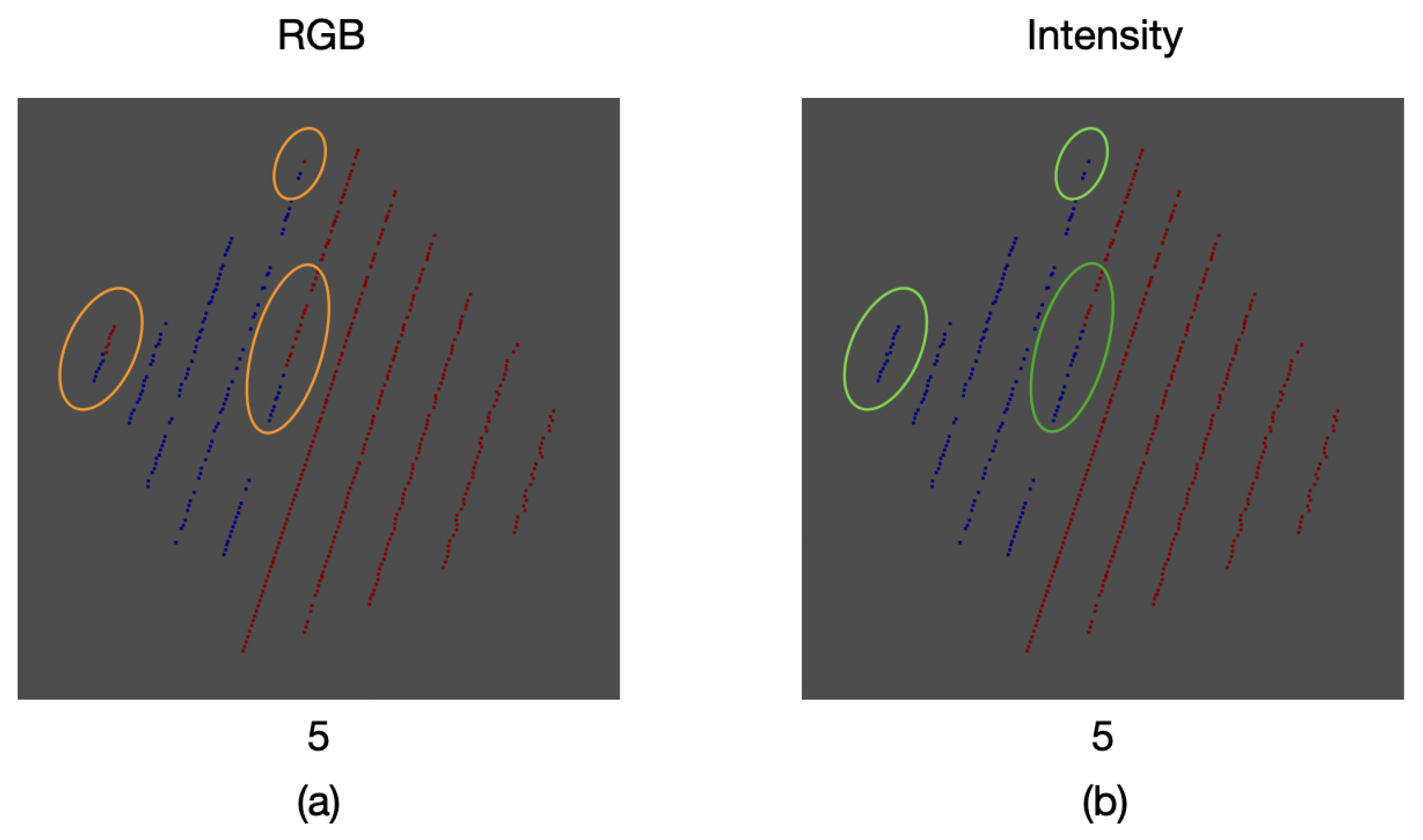
With these five complete samples (point clouds and 2D images), Algorithm 4 was applied in order to assign the corresponding color information to each point in the cloud, as shown in Figure 17a. Subsequently, using color segmentation, a thresholding stage was applied to the point clouds: points close to a black color took the value of , those close to a white color took the value of and the remaining points took the value of . Figure 17b shows the point clouds after this color thresholding stage.
After this thresholding stage, we utilized the intensity information returned by the LiDAR and compared it to the black-white classified point cloud. Figure 17c presents the point clouds with intensity information. Since the intensity returned by the LiDAR provides enough information to identify a black or white color, we applied another thresholding stage to the intensity information as presented in Figure 17d. With this information, it is now possible to compare both thresholding stages (color and intensity) in order to measure the error of the calibration method.
3.4. Four-Dimensional Phenotyping Model
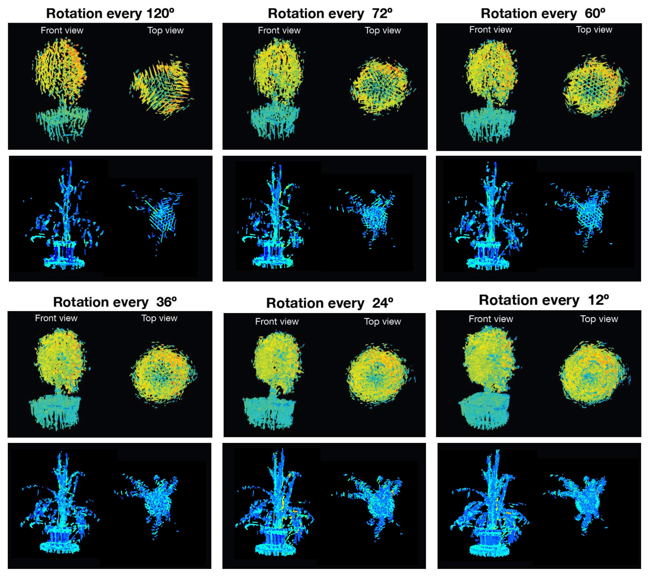
Since the main goal of this research project is the generation of complete 4D phenotyping models, an experiment was performed first to verify how the morphological and biological parameters extracted from the plant were affected by using different rotation angles at the time of sensing. For this purpose, the Limonaria and Guaiacum plants were scanned with steps of , , , , , and , simultaneously using the LiDAR and the multispectral camera. Subsequently, Algorithm 4 was executed to obtain the sensory fusion between each 3D point cloud and each multispectral camera image. By using Algorithm 7, the registration of the point clouds with color information was done, obtaining the 4D phenotyping models. The 4D phenotyping models of both Guaiacum and Limonaria plants are shown in Figure 18.
During the acquisition and analysis stages of a phenotyping platform, there are many external factors that may affect its stability, e.g., environmental conditions. With that in mind, it becomes paramount to validate the stability of the measurements in time. For this purpose, an experiment was conducted in which the Guaiacum plant was scanned during different moments of a single day, to observe how the vegetative index average behaved over time in this plant. As a result, the graph of the average NDVI of the Guaiacum plant during the day is presented in Figure 19. In order to perform a qualitative analysis of this behavior, Figure 20 presents the 4D phenotyping models of the Guaiacum plant for three different moments in the day, in which the lowest and highest values of the average NDVI were found.
Figure 19 and Figure 20 present a very interesting behavior that would not be easy to predict or validate. Although NDVI is useful for vegetation monitoring, specially because it should compensate for varying illumination conditions. Moreover, the NDVI has the advantage of weighting more the light reflectances in both NIR and green compared to other wavelengths, which enables to characterize the plant health status. Our results show that a variation of this metric indeed occurs at different hours of the day. With that limitation, the analysis process that utilizes the NDVI index would require an adjustment in order to consider this natural behavior, as presented next in the discussion section.
4. Discussion
Due to the technological limitations of the selected LiDAR, a mechanism to remove the generated noisy points was necessary. As shown in Figure 14, after averaging and filtering the point cloud, the unwanted noisy intermediate points are successfully removed, which becomes paramount for the proper registration of the point clouds.
As a result of the comparison between the intensity and color information thresholding stages, an error of was found for the proposed calibration method. This error can be seen in some of the samples where, due to the inclination of the calibration board edges, the mapped color was that of the background and not the one of the board itself. Likewise, in other areas there is not a proper match for the color of the board, as it can be seen in Figure 21.
As it can be seen in Figure 18, as we decrease the rotation step of the rotating base, there is an evident increase in the details of the morphological structure of the plant for the generated phenotyping model. Additionally, the estimated average NDVI index for the plant also tends to stabilize as the rotation step decreases.
Although the proposed system successfully generates a 4D phenotyping model of the scanned plant, it was necessary to validate the stability of these measurements. It was possible to demonstrate that the biochemical and physiological parameters of plants vary at different times of the day, due to the processes they undergo to obtain nutrients when exposed to different light and environmental conditions along the day.
Thus, as shown in Figure 19 and Figure 20, the temporal distribution of the biochemical parameters of the plant can be studied with the 4D models that are generated by the implemented platform. In this case, the results obtained show how the levels of the NDVI index of the plant have maximum at noon, when the sun rays’ intensity is also at its maximum levels. These results evince a relationship between the amount of sunlight that the plant can absorb during day hours and its vegetative indices. Furthermore, plant-health status is usually characterized throughout the entire phenological state of the crop, however, in Figure 19, we note that the NDVI index shows significant fluctuations during the day, allowing an analysis with a higher and more precise temporal resolution.
5. Conclusions
In this research work, it was shown how the use of low-density vertical LiDAR radars together with multispectral images can be successfully used for the generation of 4D phenotyping models of plants, which allows its morphological study and the temporal analysis of variables and physiological parameters, under different environmental conditions.
On the other hand, the proposed calibration board with a novel shape and color configuration eases the verification of the resulting calibration of the intrinsic and extrinsic parameters of the LiDAR and the camera. An algorithm that combines the averaging and filtering of the point cloud values was designed and implemented to remove unwanted points within the point cloud data.
Our ongoing work is focused on the generation of a surface model of the plant, utilizing the available point cloud and color information, in order to support the analysis of the 4D phenotyping model, aimed at using the calculated spatio-temporal vegetation indices as features for training machine learning models for leaf nitrogen estimation.
Author Contributions
Conceptualization, D.M., J.D.C., M.G.R.; methodology, D.M., J.D.C., M.G.R.; software, M.G.R.; validation, D.M., J.D.C., M.G.R.; formal analysis and investigation, D.M., J.D.C., M.G.R.; data curation, J.D.C., M.G.R.; writing—original draft preparation, M.G.R.; writing—review and editing, D.M., J.D.C.; supervision, D.M., J.D.C. All authors have read and agreed to the published version of the manuscript.
Funding
This work was funded by the OMICAS program: “Optimización Multiescala In-silico de Cultivos Agrícolas Sostenibles (Infraestructura y validación en Arroz y Caña de Azúcar)”, anchored at the Pontificia Universidad Javeriana in Cali and funded within the Colombian Scientific Ecosystem by The World Bank, the Colombian Ministry of Science, Technology and Innovation, the Colombian Ministry of Education, the Colombian Ministry of Industry and Tourism, and ICETEX, under grant ID: FP44842-217-2018 and OMICAS Award ID: 792-61187.
Data Availability Statement
Datasets supporting the experimental results presented in Figures are available at the Open Science Framework: https://osf.io/cde6h/?view_only=1c4e5e03b9a34d3b96736ad8ab1b2774 accessed on 29 November 2021, folder Raw Data-MDPI Remote Sensing-Special Issue 3D Modelling and Mapping for Precision Agriculture.
Acknowledgments
The authors would like to thank all CIAT staff that supported the experiments conducted above the crops located at CIAT headquarters in Palmira, Valle del Cauca, Colombia; in particular, thanks to Eliel Petro for his feedback during this project.
Conflicts of Interest
The authors declare no conflict of interest.
References
- Furbank, R.T.; Tester, M. Phenomics-technologies to relieve the phenotyping bottleneck. Trends Plant Sci. 2011, 16, 635–644. [Google Scholar] [CrossRef]
- Furbank, R.T.; Von Caemmerer, S.; Sheehy, J.; Edwards, G. C4 rice: A challenge for plant phenomics. Funct. Plant Biol. 2009, 36, 845–856. [Google Scholar] [CrossRef] [PubMed]
- Reynolds, M.; Foulkes, M.J.; Slafer, G.A.; Berry, P.; Parry, M.A.; Snape, J.W.; Angus, W.J. Raising yield potential in wheat. J. Exp. Bot. 2009, 60, 1899–1918. [Google Scholar] [CrossRef] [PubMed] [Green Version]
- Tester, M.; Langridge, P. Breeding technologies to increase crop production in a changing world. Science 2010, 327, 818–822. [Google Scholar] [CrossRef]
- Paulus, S.; Schumann, H.; Kuhlmann, H.; Léon, J. High-precision laser scanning system for capturing 3D plant architecture and analysing growth ofcereal plants. Biosyst. Eng. 2014, 121, 1–11. [Google Scholar] [CrossRef]
- Newsome, R. Feeding the future. Food Technol. 2010, 64, 48–56. [Google Scholar] [CrossRef]
- Mokarram, M.; Hojjati, M.; Roshan, G.; Negahban, S. Modeling the behavior of Vegetation Indices in the salt dome of Korsia in North-East of Darab, Fars, Iran. Model. Earth Syst. Environ. 2015, 1, 1–9. [Google Scholar] [CrossRef] [Green Version]
- Apelt, F.; Breuer, D.; Nikoloski, Z.; Stitt, M.; Kragler, F. Phytotyping4D: A light-field imaging system for non-invasive and accurate monitoring of spatio-temporal plant growth. Plant J. 2015, 82, 693–706. [Google Scholar] [CrossRef]
- Donald, M.R.; Mengersen, K.L.; Young, R.R. A Four Dimensional Spatio-Temporal Analysis of an Agricultural Dataset. PLoS ONE 2015, 10, e0141120. [Google Scholar] [CrossRef] [Green Version]
- Luo, R.C.; Yih, C.C.; Su, K.L. Multisensor fusion and integration: Approaches, applications, and future research directions. IEEE Sens. J. 2002, 2, 107–119. [Google Scholar] [CrossRef]
- Hosoi, F.; Umeyama, S.; Kuo, K. Estimating 3D chlorophyll content distribution of trees using an image fusion method between 2D camera and 3D portable scanning lidar. Remote Sens. 2019, 11, 2134. [Google Scholar] [CrossRef] [Green Version]
- Sun, G.; Ding, Y.; Wang, X.; Lu, W.; Sun, Y.; Yu, H. Nondestructive determination of nitrogen, phosphorus and potassium contents in greenhouse tomato plants based on multispectral three-dimensional imaging. Sensors 2019, 19, 5295. [Google Scholar] [CrossRef] [PubMed] [Green Version]
- Itakura, K.; Kamakura, I.; Hosoi, F. Three-dimensional monitoring of plant structural parameters and chlorophyll distribution. Sensors 2019, 19, 413. [Google Scholar] [CrossRef] [Green Version]
- Häming, K.; Peters, G. The structure-from-motion reconstruction pipeline—A survey with focus on short image sequences. Kybernetika 2010, 46, 926–937. [Google Scholar]
- Zhang, J.; Li, Y.; Xie, J.; Li, Z. Research on optimal near-infrared band selection of chlorophyll (SPAD) 3D distribution about rice PLANT. Spectrosc. Spectr. Anal. 2017, 37, 3749–3757. [Google Scholar]
- El Hazzat, S.; Saaidi, A.; Satori, K. Multi-view passive 3D reconstruction: Comparison and evaluation of three techniques and a new method for 3D object reconstruction. In Proceedings of the International Conference on Next Generation Networks and Services, NGNS, Casablanca, Morocco, 28–30 May 2014; pp. 194–201. [Google Scholar] [CrossRef]
- Pérez-Ruiz, M.; Prior, A.; Martinez-Guanter, J.; Apolo-Apolo, O.E.; Andrade-Sanchez, P.; Egea, G. Development and evaluation of a self-propelled electric platform for high-throughput field phenotyping in wheat breeding trials. Comput. Electron. Agric. 2020, 169, 105237. [Google Scholar] [CrossRef]
- Jimenez-Berni, J.A.; Deery, D.M.; Rozas-Larraondo, P.; Condon, A.T.G.; Rebetzke, G.J.; James, R.A.; Bovill, W.D.; Furbank, R.T.; Sirault, X.R. High throughput determination of plant height, ground cover, and above-ground biomass in wheat with LiDAR. Front. Plant Sci. 2018, 9, 1–18. [Google Scholar] [CrossRef] [Green Version]
- Thapa, S.; Zhu, F.; Walia, H.; Yu, H.; Ge, Y. A novel LiDAR-Based instrument for high-throughput, 3D measurement of morphological traits in maize and sorghum. Sensors 2018, 18, 1187. [Google Scholar] [CrossRef] [Green Version]
- Sun, G.; Wang, X.; Sun, Y.; Ding, Y.; Lu, W. Measurement method based on multispectral three-dimensional imaging for the chlorophyll contents of greenhouse tomato plants. Sensors 2019, 19, 3345. [Google Scholar] [CrossRef] [Green Version]
- Park, Y.; Yun, S.; Won, C.S.; Cho, K.; Um, K.; Sim, S. Calibration between color camera and 3D LIDAR instruments with a polygonal planar board. Sensors 2014, 14, 5333–5353. [Google Scholar] [CrossRef] [Green Version]
- Debattisti, S.; Mazzei, L.; Panciroli, M. Automated extrinsic laser and camera inter-calibration using triangular targets. IEEE Intell. Veh. Symp. Proc. 2013, 696–701. [Google Scholar] [CrossRef] [Green Version]
- Hurtado-ramos, J.B. LIDAR and Panoramic Camera Extrinsic. In Lecture Notes in Computer Science (LNCS); Springer: Berlin/Heidelberg, Germany, 2013; pp. 104–113. [Google Scholar]
- Li, J.; He, X.; Li, J. 2D LiDAR and camera fusion in 3D modeling of indoor environment. In Proceedings of the IEEE National Aerospace Electronics Conference, NAECON 2016, Dayton, OH, USA, 26–29 July 2016; pp. 379–383. [Google Scholar] [CrossRef]
- Zhou, L.; Deng, Z. Extrinsic calibration of a camera and a lidar based on decoupling the rotation from the translation. IEEE Intell. Veh. Symp. Proc. 2012, 642–648. [Google Scholar] [CrossRef]
- Silva, V.D.; Roche, J.; Kondoz, A. Robust Fusion of LiDAR and Wide-Angle Camera. Sensors 2018, 18, 2730. [Google Scholar] [CrossRef] [PubMed] [Green Version]
- Rodriguez F., S.A.; Frémont, V.; Bonnifait, P. Extrinsic calibration between a multi-layer lidar and a camera. In Proceedings of the IEEE International Conference on Multisensor Fusion and Integration for Intelligent Systems, Seoul, Korea, 20–22 August 2008; pp. 214–219. [Google Scholar] [CrossRef] [Green Version]
- Ardeshir, A. 2-D and 3-D Image Registration, 1st ed.; John Wiley & Sons: Hoboken, NJ, USA, 2005. [Google Scholar]
- Luo, P.; Liao, J.; Shen, G. Combining Spectral and Texture Features for Estimating Leaf Area Index and Biomass of Maize Using Sentinel-1/2, and Landsat-8 Data. IEEE Access 2020, 8, 53614–53626. [Google Scholar] [CrossRef]
- Harrell, D.; Tubana, B.; Walker, T.; Phillips, S. Estimating rice grain yield potential using normalized difference vegetation index. Agron. J. 2011, 103, 1717–1723. [Google Scholar] [CrossRef]
- Viljanen, N.; Honkavaara, E.; Näsi, R.; Hakala, T.; Niemeläinen, O.; Kaivosoja, J. A novel machine learning method for estimating biomass of grass swards using a photogrammetric canopy height model, images and vegetation indices captured by a drone. Agriculture 2018, 8, 70. [Google Scholar] [CrossRef] [Green Version]
Figure 1.
The selected embedded system and sensors (a) Jetson TX2 (b) VLP-16 LiDAR (c) Sequoia camera.
Figure 1.
The selected embedded system and sensors (a) Jetson TX2 (b) VLP-16 LiDAR (c) Sequoia camera.

Figure 2.
Mechanical structure for the 4D phenotyping platform.

Figure 3.
Plants used for the experimentation stages of this work: (A) The Limonaria (Cymbopogon citratus), (B) The Guaiacum bonsai (Cuaiacum officinale).
Figure 3.
Plants used for the experimentation stages of this work: (A) The Limonaria (Cymbopogon citratus), (B) The Guaiacum bonsai (Cuaiacum officinale).

Figure 4.
General architecture of the proposed 4D phenotyping system.
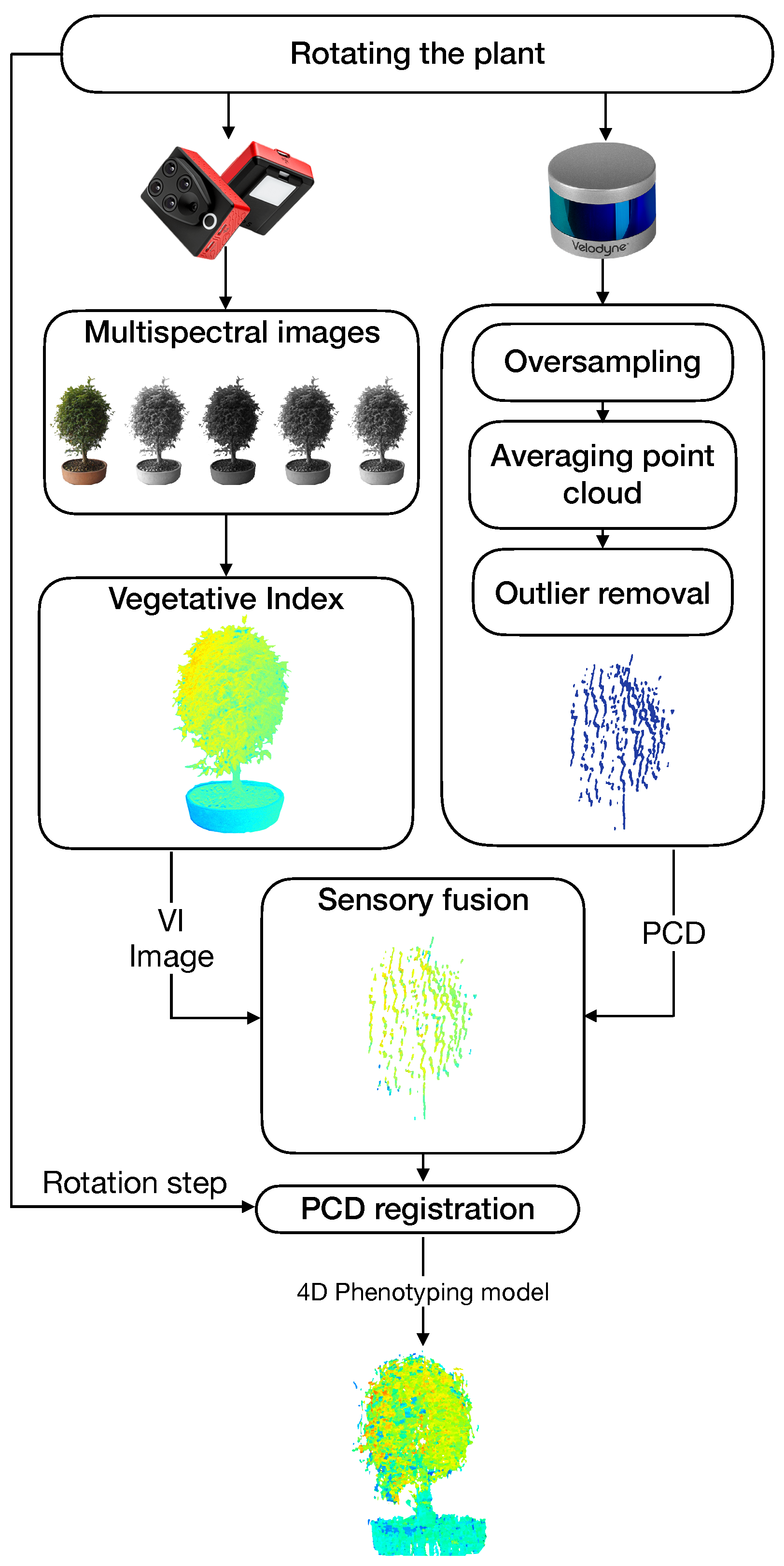
Figure 5.
Unwanted points returned by the VLP-16 LiDAR. (a) Object sensed by the LiDAR. (b) Point cloud (side view) returned by the LiDAR. (c) Unwanted points in red. (d) Expected filtered result.
Figure 5.
Unwanted points returned by the VLP-16 LiDAR. (a) Object sensed by the LiDAR. (b) Point cloud (side view) returned by the LiDAR. (c) Unwanted points in red. (d) Expected filtered result.

Figure 6.
Behavior of the LiDAR’s lasers when they hit the edges of an object and another object is behind it.
Figure 6.
Behavior of the LiDAR’s lasers when they hit the edges of an object and another object is behind it.
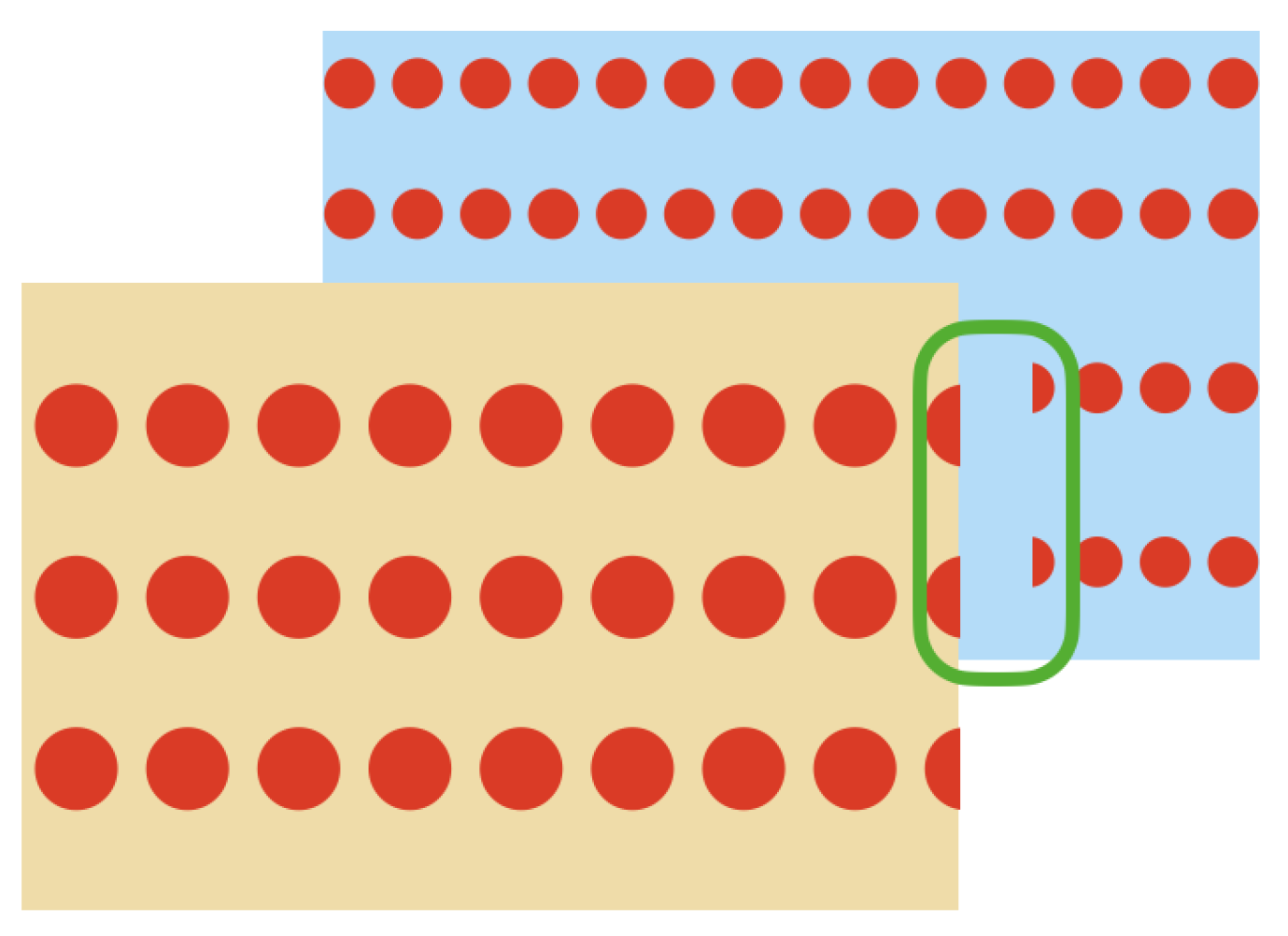
Figure 7.
Point cloud oversampling and filtering diagram.

Figure 8.
Proposed board for calibration between 2D and 3D data.

Figure 9.
Acquired 3D points belonging to the calibration board and their projection on an estimated plane P.
Figure 9.
Acquired 3D points belonging to the calibration board and their projection on an estimated plane P.

Figure 10.
3D points belonging to the calibration point, the corresponding estimated edges, and the resulting key points.
Figure 10.
3D points belonging to the calibration point, the corresponding estimated edges, and the resulting key points.

Figure 11.
Origin point of the LiDAR coordinate system and the axis of rotation of the rotating base.
Figure 11.
Origin point of the LiDAR coordinate system and the axis of rotation of the rotating base.

Figure 12.
Result of the estimation of vegetative indexes in the Limonaria plant.
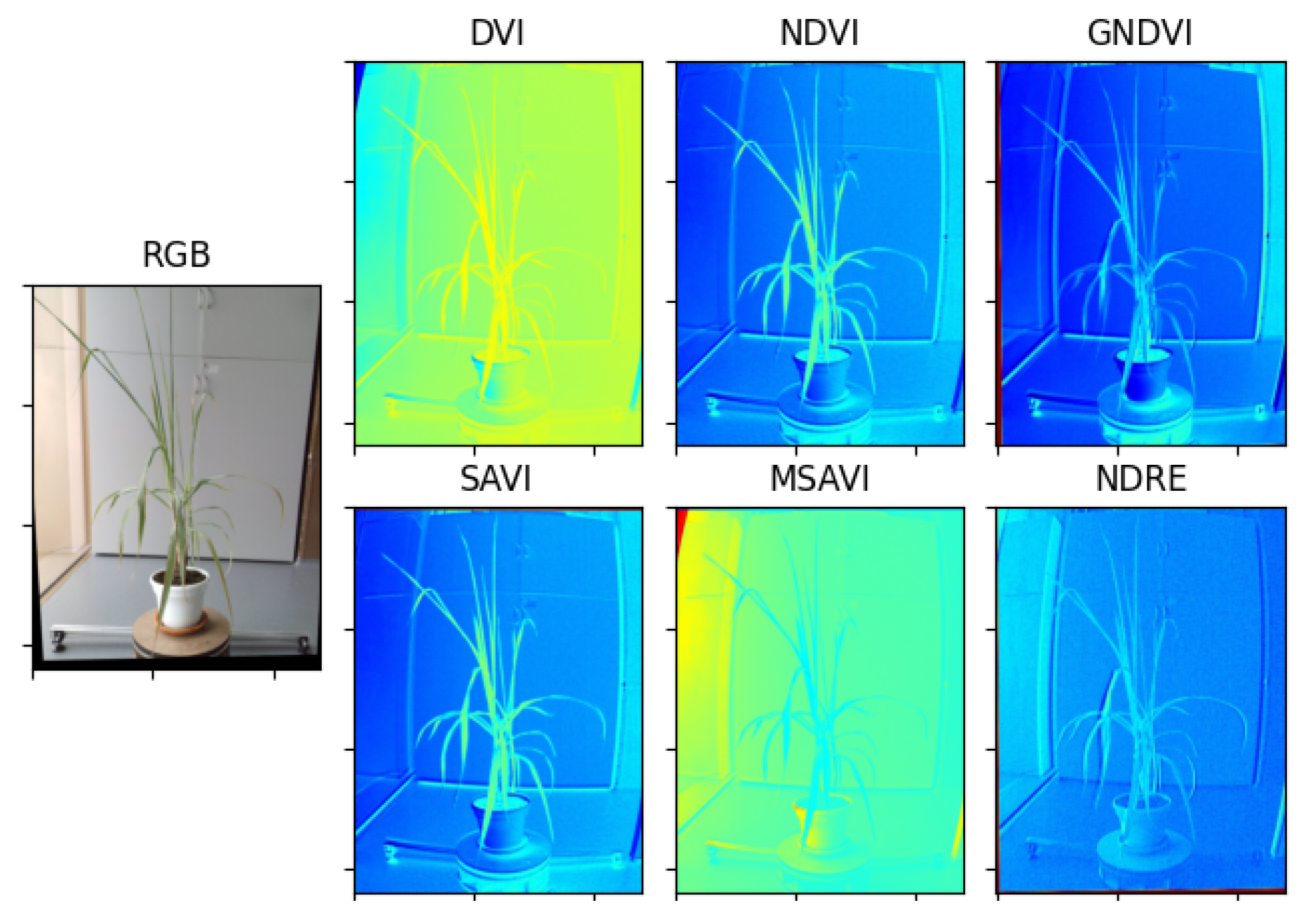
Figure 13.
Result of the estimation of vegetative indexes in the Guayacan plant.

Figure 14.
Oversampling and outlier removal on the the point clouds. (a) Raw point cloud of the Limonaria plant. (b) Regions of the point cloud where unwanted points are found (in red). (c) Point cloud after oversampling, averaging, and filtering.
Figure 14.
Oversampling and outlier removal on the the point clouds. (a) Raw point cloud of the Limonaria plant. (b) Regions of the point cloud where unwanted points are found (in red). (c) Point cloud after oversampling, averaging, and filtering.

Figure 15.
2D key point extraction process.

Figure 16.
Key points estimation in a 3D point cloud. (a) Point cloud of the calibration board. (b) Extraction of points belonging to the edges of the calibration board. (c) Edge lines intersection and estimated key points. (d) Projection of the key points into the 3D space.
Figure 16.
Key points estimation in a 3D point cloud. (a) Point cloud of the calibration board. (b) Extraction of points belonging to the edges of the calibration board. (c) Edge lines intersection and estimated key points. (d) Projection of the key points into the 3D space.

Figure 17.
Point cloud processing. (a) Color information, (b) Color thresholding stage. (c) Intensity information. (d) Intensity thresholding stage.
Figure 17.
Point cloud processing. (a) Color information, (b) Color thresholding stage. (c) Intensity information. (d) Intensity thresholding stage.
Figure 18.
4D phenotyping models captured at different rotation angles.

Figure 19.
Average vegetative index NDVI of the Guaiacum plant during the day.
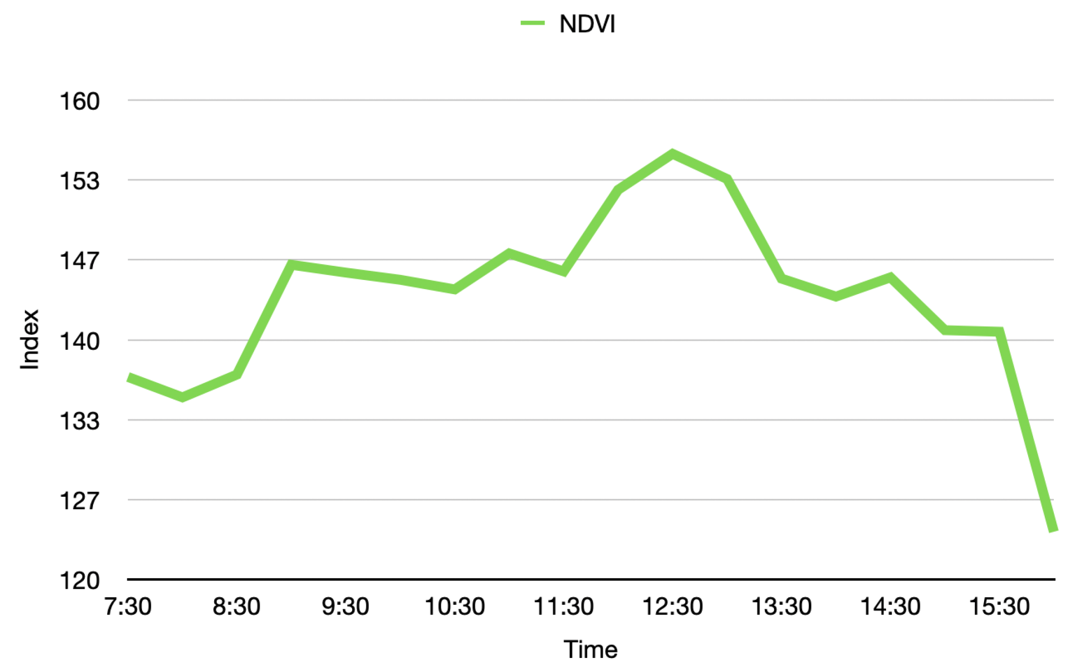
Figure 20.
4D phenotyping models of the Guaiacum plant in the three hours of the day where it had the lowest and highest peaks.
Figure 20.
4D phenotyping models of the Guaiacum plant in the three hours of the day where it had the lowest and highest peaks.
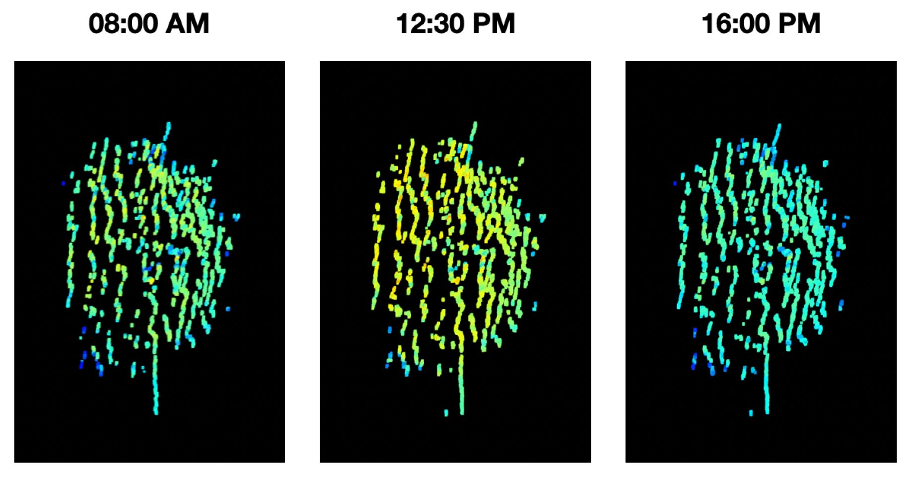
Figure 21.
Comparison between thresholding stages: (a) RGB color information, (b) intensity information. Some areas with wrongly mapped points are highlighted.
Figure 21.
Comparison between thresholding stages: (a) RGB color information, (b) intensity information. Some areas with wrongly mapped points are highlighted.

Publisher’s Note: MDPI stays neutral with regard to jurisdictional claims in published maps and institutional affiliations. |
© 2022 by the authors. Licensee MDPI, Basel, Switzerland. This article is an open access article distributed under the terms and conditions of the Creative Commons Attribution (CC BY) license (https://creativecommons.org/licenses/by/4.0/).
Share and Cite
MDPI and ACS Style
Rincón, M.G.; Mendez, D.; Colorado, J.D. Four-Dimensional Plant Phenotyping Model Integrating Low-Density LiDAR Data and Multispectral Images. Remote Sens. 2022, 14, 356. https://doi.org/10.3390/rs14020356
AMA Style
Rincón MG, Mendez D, Colorado JD. Four-Dimensional Plant Phenotyping Model Integrating Low-Density LiDAR Data and Multispectral Images. Remote Sensing. 2022; 14(2):356. https://doi.org/10.3390/rs14020356
Chicago/Turabian StyleRincón, Manuel García, Diego Mendez, and Julian D. Colorado. 2022. "Four-Dimensional Plant Phenotyping Model Integrating Low-Density LiDAR Data and Multispectral Images" Remote Sensing 14, no. 2: 356. https://doi.org/10.3390/rs14020356
Note that from the first issue of 2016, this journal uses article numbers instead of page numbers. See further details here.