An Improved Fast Estimation of Satellite Phase Fractional Cycle Biases

Abstract

Satellite phase fractional cycle biases (FCBs) are crucial to precise point positioning with ambiguity resolution (PPP–AR), and they can improve the accuracy and reliability of a solution. Traditional methods need multiple iterations and need to keep the same reference when estimating satellite phase fractional cycle biases. In this paper, we propose an improved fast estimation of FCB, which does not need any iterations and can select any reference when estimating FCB. We compare the suitability and precision of a traditional and a proposed method by BDS-3 experiments. The results of the FCB experiments show that the calculated time of the proposed method is less than the traditional method and that computation efficiency is increased by 34.71%. These two methods have a similar rate of fixed epochs and ambiguities in the static and dynamic models. However, the time to first fix (TTFF) of the proposed method decreased by 19.69% and 28.83% for the static and dynamic models, respectively. The results show that the proposed method has a better convergence time in PPP–AR.

1. Introduction

The International Geodesy Service (IGS) is an international organization established by the International Association of Geodesy to support geodetic and geodynamic research. In the mid-1990s, IGS began to provide precise orbit and clock products for users around the world, which made it possible for the realization of PPP based on an undifferenced model. Zumberge et al. [1] realized a centimeter-level static PPP through the ionosphere-free (IF) combined model, which used precise ephemeris and clock products provided by IGS. It was verified through experiments that it is completely feasible to use undifferenced observations for PPP in theory. Héroux et al. [2] also obtained centimeter-level positioning accuracy by using a dual-frequency ionosphere-free (IF) combined model in PPP. Ye et al. [3] analyzed the PPP models and discussed the final and real-time PPP models based on a network. Gao et al. [4] proposed the UofC model, which significantly mitigated the problem of large observation noise in the IF model and reduced the convergence time of PPP.

With the advantage of more redundant observations and better satellite spatial geometry, multi-GNSS combinations can reduce convergence time and improve the positioning accuracy of PPP. Some research shows that it can effectively speed up the convergence of PPP by adding the satellites of GLONASS. The effect is obvious in improving the accuracy of static positioning, but the effect is not obvious in improving the accuracy of dynamic positioning [5,6,7,8,9]. In 2011, IGS started the Multi-GNSS Experiment (MGEX) program with the purpose of observing, collecting, and analyzing multi-GNSS data, providing precise products and services [10]. With the completion of BDS-3 in 2020, there are four global satellite navigation systems (GPS, GLONASS, BDS, and Galileo) and two regional satellite navigation systems (QZSS and IRNSS). Multi-GNSS PPP–AR has become a developmental trend for precise positioning [11]. As an important part of GNSS, it is necessary to ensure the validity of BDS-3 PPP–AR in the long run. In other words, we need to ensure that the FCB is precise and available in the long run.

Traditional PPP technology still has problems such as long convergence time and low accuracy. The PPP fixed solution can greatly improve positioning accuracy and shorten convergence time. The key to PPP–AR is to separate the FCB between receivers and satellites and then recover the integer characteristics of ambiguity. Gabor et al. [12] decomposed the IF-combined ambiguity into wide-lane (WL) and narrow-lane (NL) ambiguities with integer characteristics and then used the GPHASE function to separate FCBs from the ambiguities. They then tried to solve the WL and NL single-differenced FCBs between satellites. However, due to the limitation of the precise ephemeris and clock products at that time, only the WL FCB could be effectively separated. Due to the improved accuracy of IGS precise products, Ge et al. [13] used the single-differenced model to estimate WL and NL FCB and successfully fixed the single-differenced ambiguities. Zhang et al. [14] used the least square method to estimate the undifferenced FCBs between receivers and satellites by constructing the observation equations of the undifferenced FCBs. Laurichesse et al. [15] proposed the Integer Phase Clock (IPC), where the NL FCB is sucked into the satellite clock error to form the IPC, and users can fix the ambiguities by using IPC. Collons et al. [16] proposed the Decoupled Clock (DC) method on the basis of IPC to estimate the satellite pseudorange and phase clock errors at the same time. Geng. et al. and Shi et al. [17,18] proved the equivalence of FCB, IPC, and DC through experiments. However, the IPC and DC methods are complicated and difficult because we need to estimate the satellite clock errors. It is hard for most researchers to estimate satellite clock errors. The estimation of the FCB method has the advantages of a simple model, easy algorithm programming, and mature theory, and it is easy to use for users. It can adapt to the orbit and clock error products of different analysis centers for users. Therefore, we used the FCB method to estimate the BDS-3 FCB in this paper. The traditional method requires several iterative calculations and takes a long time to obtain a convergent solution when estimating NL FCB [14,19,20] because the iterative condition of NL FCB is that the fixed NL ambiguities are not changed. For real-time PPP (RT–PPP), users need state-space representation (SSR). They also need FCB for ambiguity-resolved real-time PPP (AR–RT–PPP). The real-time data are generally delayed during processing or transmission. The research shows that if the time of transmission is longer, the precision of PPP is lower. In addition, the precision of PPP can significantly decrease when the time of transmission is longer than 20 seconds [21]. Especially for the users of AR–RT–PPP, it is also important to speed up the computational efficiency of FCB. In order to speed up the convergence of the algorithm, some researchers proposed an initial value of NL FCB by traversing all stations. However, it also needs several times to iterate the initial value in order to obtain precise NL FCB, because the lower precise initial value of NL FCB cannot fixed all NL ambiguities correctly.

In this paper, an improved FCB method of estimation is proposed, and we test the performance of this method under different models by using BDS-3. The second section analyzes the PPP model and the error sources of BDS-3. The third section introduces the traditional BDS-3 WL and NL FCB methods of estimation and then proposes an improved FCB method of estimation. The fourth section shows an analysis of the stability and accuracy of the BDS-3 WL and NL FCB. Then, we analyze the performance of FCB through static and dynamic PPP–AR experiments by using the proposed method.

2. Methods

2.1. PPP Model of BDS-3

The BDS-3 pseudorange and carrier phase observation equation can be expressed as

$$\begin{array}{l}{P}_{r,i}^s={\rho }_r^s+cd{t}_r-cd{t}^s+{\gamma }_i{I}_{r,1}^s+T_r^s+b_{r,i}-b_i^s+{\epsilon }_{r,i}^s\\ L_{r,i}^s={\rho }_r^s+cd{t}_r-cd{t}^s-{\gamma }_i{I}_{r,1}^s+T_r^s+{\lambda }_i\left(N_{r,i}^s+{\psi }_{r,i}+{\varphi }_{r,i}-{\psi }_i^s-{\varphi }_i^s\right)+{\delta }_{r,i}^s\end{array}$$

(1)

where s, i, and r, respectively denote the SV number of a satellite’s system, frequency, and receiver. $P_{r,i}^s$ and $L_{r,i}^s$ are the pseudorange and carrier phase observation values (m), respectively. ${\rho }_r^s$ is the Euclidean distance between the satellite and receiver. $d{t}_r$ and $d{t}^s$ are receiver and satellite errors, respectively. c is the speed of light. ${\gamma }_i=f_1^2/f_i^2$ is ionospheric mapping factor. $I_{r,1}^s$ is the ionospheric delay at the first frequency. $T_r^s$ is the tropospheric delay. $b_{r,i}$ and $b_i^s$ are the receiver and satellite pseudorange hardware delay, respectively. $N_{r,i}^s$ is the carrier phase integer ambiguity. ${\varphi }_{r,i}$ and ${\varphi }_i^s$ are the receiver and satellite of initial phase shift, respectively. ${\psi }_{r,i}$ and ${\psi }_i^s$ are the receiver and satellite phase hardware delay, respectively. We merged the initial phase shift and phase hardware delay and the so-called uncalibrated phase delays (UPD) because they cannot be separated. The receiver and satellite UPD can be described as ${\phi }_{r,i}={\psi }_{r,i}+{\varphi }_{r,i}$ and ${\phi }_i^s={\psi }_i^s+{\varphi }_i^s$. The fractional part of UPD is called phase fractional cycle biases (FCB). It is the reason that the ambiguities are not integers in PPP. ${\epsilon }_{r,i}^s$ and ${\delta }_{r,i}^s$ are the other unmodeled errors of pseudorange and carrier, such as observation noise and multipath errors. These errors can be decreased by long smoothing. In the above equation, the antenna phase center correction, relativistic effect, tide loading correction (solid tide, extreme tide, and ocean tide), Sagnac effect, satellite antenna phase wind-up, and other corrections at the satellite and receiver are not included. These corrections were applied by appropriate models in advance [22].

The dual-frequency IF combination commonly used in PPP eliminates the effect of the first-order ionospheric delay. The pseudorange and carrier phase IF combination of frequencies i and j can be expressed as

$$\{\begin{array}{l}{P}_{r,IF}^s={\alpha }_{ij}·P_{r,i}^s+{\beta }_{ij}{P}_{r,j}^s\\ L_{r,IF}^s={\alpha }_{ij}·L_{r,i}^s+{\beta }_{ij}{L}_{r,j}^s\end{array}$$

(2)

where ${\alpha }_{ij}$ and ${\beta }_{ij}^{}$ are IF combination coefficients.

$${\alpha }_{ij}=\frac{f_i^2}{f_i^2-f_j^2},{\beta }_{ij}^{}=-\frac{f_j^2}{f_i^2-f_j^2}$$

(3)

Then, the IF observation model corresponding to Equation (1) can be written as

$$\{\begin{array}{l}{P}_{r,\mathrm{I}\mathrm{F}}^s={\rho }_r^s+d{t}_r-d{t}^s+T_r^s+b_{r,\mathrm{I}\mathrm{F}}-b_{IF}^s+{\epsilon }_{r,\mathrm{I}\mathrm{F}}^s\\ L_{r,\mathrm{I}\mathrm{F}}^s={\rho }_r^s+d{t}_r-d{t}^s+T_r^s+{\lambda }_{IF}\left(N_{r,\mathrm{I}\mathrm{F}}^s+{\phi }_{r,\mathrm{I}\mathrm{F}}-{\phi }_{IF}^s\right)+{\delta }_{r,\mathrm{I}\mathrm{F}}^s\end{array}$$

(4)

Then,

$$\{\begin{array}{l}{b}_{r,\mathrm{I}\mathrm{F}}={\alpha }_{ij}{b}_{r,i}+{\beta }_{ij}{b}_{r,j}\\ b_{IF}^s={\alpha }_{ij}{b}_i^s+{\beta }_{ij}{b}_j^s\\ N_{r,\mathrm{I}\mathrm{F}}^s=\left({\alpha }_{ij}{\lambda }_i{N}_{r,i}^s+{\beta }_{ij}{\lambda }_j{N}_{r,j}^s\right)/{\lambda }_{IF}\\ {\phi }_{r,\mathrm{I}\mathrm{F}}=\left({\alpha }_{ij}{\lambda }_i{\phi }_{r,i}+{\beta }_{ij}{\lambda }_j{\phi }_j\right)/{\lambda }_{IF}\\ {\phi }_{IF}^s=\left({\alpha }_{ij}{\lambda }_i{\phi }_i^s+{\beta }_{ij}{\lambda }_j{\phi }_i^s\right)/{\lambda }_{IF}\\ {\widehat{N}}_{r,\mathrm{I}\mathrm{F}}^s=N_{r,\mathrm{I}\mathrm{F}}^s+{\phi }_{r,\mathrm{I}\mathrm{F}}-{\phi }_{IF}^s\\ {\lambda }_{IF}=c/({\alpha }_{ij}{f}_i+{\beta }_{ij}{f}_j)\end{array}$$

(5)

where $b_{r,\mathrm{I}\mathrm{F}}$ and $b_{IF}^s$ are the IF combination of receiver and satellite pseudorange hardware delay, respectively. $N_{r,\mathrm{I}\mathrm{F}}^s$, ${\phi }_{r,\mathrm{I}\mathrm{F}}$, and ${\phi }_{IF}^s$ are the IF combination of carrier phase integer ambiguity, receiver, and satellite UPD, respectively. ${\widehat{N}}_{r,\mathrm{I}\mathrm{F}}^s$ is the IF float ambiguity. ${\lambda }_{IF}$ is the IF wavelength, and it is also the L1 wavelength.

It can be seen from Equations (4) and (5) that the IF ambiguity does not have integer characteristics. In order to obtain the fixed solution by using the IF model in PPP, the IF float ambiguity is generally decomposed into the linear combination of WL and NL integer ambiguity (i = 1, j = 2) as follows:

$$N_{r,\mathrm{I}\mathrm{F}}^s=\left(\frac{c{f}_2}{f_1^2-f_2^2}{N}_{r,WL}^s+\frac{c}{f_1+f_2}{\widehat{N}}_{r,NL}^s\right)/{\lambda }_{IF}$$

(6)

where $N_{r,WL}^s$ is WL integer ambiguity. WL float ambiguity is generally calculated by MW combination [23,24].

$$\begin{array}{ll}{\widehat{N}}_{r,WL}^s& =\left[\left(f_1{L}_{r,1}^s-f_2{L}_{r,2}^s\right)/\left(f_1-f_2\right)-\left(f_1{P}_{r,1}^s-f_2{P}_{r,2}^s\right)/\left(f_1+f_2\right)\right]/{\lambda }_{IF}\\ & =N_{r,WL}^s+{\phi }_{r,WL}^{}-{\phi }_{WL}^s\end{array}$$

(7)

$${\phi }_{r,WL}={\phi }_{r,1}-{\phi }_{r,2}-\left(f_1{b}_{r,1}+f_2{b}_{r,2}\right)/\left(f_1+f_2\right)/{\lambda }_{WL}$$

(8)

$${\phi }_{WL}^s={\phi }_1^s-{\phi }_2^s-\left(f_1{b}_1^s+f_2{b}_2^s\right)/\left(f_1+f_2\right)/{\lambda }_{WL}$$

(9)

where ${\widehat{N}}_{r,WL}^s$ is WL float ambiguity. ${\lambda }_{WL}$ is WL wavelength. The influence of multipath errors can be decreased by smoothing MW ambiguities in the long run. It can be seen from Equation (7) that the WL ambiguity $N_{r,WL}^s$ can be fixed by eliminating ${\phi }_{r,WL}^{}$ and ${\phi }_{WL}^s$. When the WL ambiguity is fixed, the NL ambiguity can be expressed as the combination of IF ambiguity and WL ambiguity as follows:

$$\begin{array}{ll}{\widehat{N}}_{r,NL}^s& ={\lambda }_{IF}\left(f_1+f_2\right){\widehat{N}}_{r,IF}^s/c-f_2\left(f_1-f_2\right)N_{r,WL}^s\\ & =N_{r,1}^s+{\phi }_{r,NL}^{}-{\phi }_{NL}^s\end{array}$$

(10)

$$\begin{array}{ll}{\phi }_{r,NL}^{}& =\left(f_1+f_2\right)/c\left({\phi }_{r,IF}{\lambda }_{IF}-b_{r,IF}\right)\\ & =f_1\left(f_1-f_2\right)\left({\phi }_{r,1}-b_{r,1}/{\lambda }_1\right)-f_2\left(f_1-f_2\right)\left({\phi }_{r,2}-b_{r,2}/{\lambda }_2\right)\end{array}$$

(11)

$$\begin{array}{ll}{\phi }_{NL}^s& =\left(f_1+f_2\right)/c\left({\phi }_{IF}^s{\lambda }_{IF}-b_{IF}^s\right)\\ & =f_1\left(f_1-f_2\right)\left({\phi }_1^s-b_1^s/{\lambda }_1\right)-f_2\left(f_1-f_2\right)\left({\phi }_2^s-b_2^s/{\lambda }_2\right)\end{array}$$

(12)

where ${\widehat{N}}_{r,NL}^s$ is the linear combination of $N_{r,1}^s$, pseudorange hardware delay, and phase delay. Since the coefficient of $N_{r,NL}^s$ in Equation (6) is the wavelength of NL ambiguity, $N_{r,NL}^s$ is also called the NL ambiguity. It can be seen from Equation (10) that the NL ambiguity $N_{r,NL}^s$ can be fixed by eliminating ${\phi }_{r,NL}^{}$ and ${\phi }_{NL}^s$.

The IF ambiguity with integer ambiguity accuracy can be obtained after recombining fixed WL ambiguity and NL ambiguity into IF ambiguity. PPP–AR can be achieved by using the IF model. Therefore, it is key to successfully fixing the WL ambiguity and NL ambiguity.

2.2. Improved Fast Estimation of FCB

2.2.1. Estimation of WL FCB

From Equation (7), we can see that the WL float ambiguity can be obtained by MW combination, which can be written as follows:

$${\widehat{N}}_{r,WL}^s=N_{r,WL}^s+{\phi }_{r,WL}^{}-{\phi }_{WL}^s$$

(13)

where ${\phi }_{r,WL}^{}$ and ${\phi }_{WL}^s$ are the receiver and satellite FCB, respectively. Generally, in PPP–AR, ambiguity is fixed by the single difference between satellites, and ${\phi }_{r,WL}^{}$ can be eliminated by the single-difference model. However, the single-difference FCB, which involves the conversion of the reference satellite, is not conducive to the user side. Therefore, the satellite and receiver FCB were estimated by using the undifferenced method in the paper.

Then, Equation (8) can be rewritten as

$$R_r^s\equiv {\widehat{N}}_{r,WL}^s-\mathrm{int}\left[{\widehat{N}}_{r,WL}^s\right]={\phi }_{r,WL}^{}-{\phi }_{WL}^s$$

(14)

where $R_r^s$ is the fractional part of WL float ambiguity. $\mathrm{int}[ ]$ is the rounding symbol. Assuming that m satellites are observed by n stations, the float ambiguities of each station-satellite continuous arc can be combined into the following equations:

$$\underset{R_0}{\underbrace{\left[\begin{array}{c}\begin{array}{l}{R}_1^1\\ ⋮\end{array}\\ R_1^m\\ R_2^1\\ \begin{array}{l}⋮\\ R_2^m\\ ⋮\\ R_n^1\\ ⋮\\ R_n^m\end{array}\end{array}\right]}}=\underset{A_0}{\underbrace{\left[\begin{array}{ccccccc}1& 0& \cdots & 0& -1& \cdots & 0\\ ⋮& ⋮& ⋮& ⋮& ⋮& ⋮& ⋮\\ 1& 0& \ddots & 0& 0& \cdots & -1\\ 0& 1& \cdots & 0& -1& \cdots & 0\\ ⋮& ⋮& ⋮& ⋮& ⋮& \ddots & ⋮\\ 0& 1& \cdots & 0& 0& \cdots & -1\\ \cdots & \cdots & \cdots & \cdots & \cdots & \cdots & \cdots \\ 0& 0& \cdots & 1& -1& \cdots & 0\\ ⋮& ⋮& ⋮& ⋮& ⋮& \cdots & ⋮\\ 0& 0& \cdots & 1& 0& \cdots & -1\end{array}\right]}}\underset{X}{\underbrace{\left[\begin{array}{l}{\phi }_1\\ {\phi }_2\\ ⋮\\ {\phi }_n\\ {\phi }^1\\ ⋮\\ {\phi }^m\end{array}\right]}}$$

(15)

Due to the linear correlation between the WL FCB at the receiver and satellite in Equation (15), the equation system is rank deficient, and the rank deficient number is 1. There are three commonly used methods to solve the rank deficit: (1) choose a receiver FCB to 0; (2) choose a satellite FCB to 0; (3) the sum of all satellite FCB is 0. The three reference data are theoretically equivalent. In this paper, we selected (3), then

$${\phi }^1+{\phi }^2+\cdots +{\phi }^m=0$$

(16)

Combining Equations (15) and (16) allows us to write it in matrix form as

$$\underset{R}{\underbrace{\left[\begin{array}{l}{R}_0\\ 0\end{array}\right]}}=\underset{A}{\underbrace{\left[\begin{array}{l}{A}_0\\ A_1\end{array}\right]}}X$$

(17)

where $A$ is the design matrix of the observation equation of FCB, and $A_1=\left[\begin{array}{ccccccc}0& 0& \cdots & 0& 1& \cdots & 1\end{array}\right]$ is the design matrix of a gravity reference. Then, the receiver and satellite WL FCB can be calculated by least squares as follows:

$$X={\left(A^{\mathrm{T}}PA\right)}^{-1}{A}^{\mathrm{T}}PR$$

(18)

In Equation (18), the weight matrix $P$ can be determined by the variance of the float WL ambiguity in continuous arcs. In order to improve the robustness and accuracy of the solution, the IGG3 method can be used for iterative calculations. There are some points that should be noted when calculating the WL FCB—namely,(1) the observation time of WL float ambiguity is not less than 45 min in a continuous arc; (2) the WL float ambiguity in the arc can be averaged to reduce the influence of observation noise and multipath; (3) for ambiguities with residuals greater than 0.5 cycles, the corresponding integer ambiguity can be adjusted to perform ±1 cycles operation.

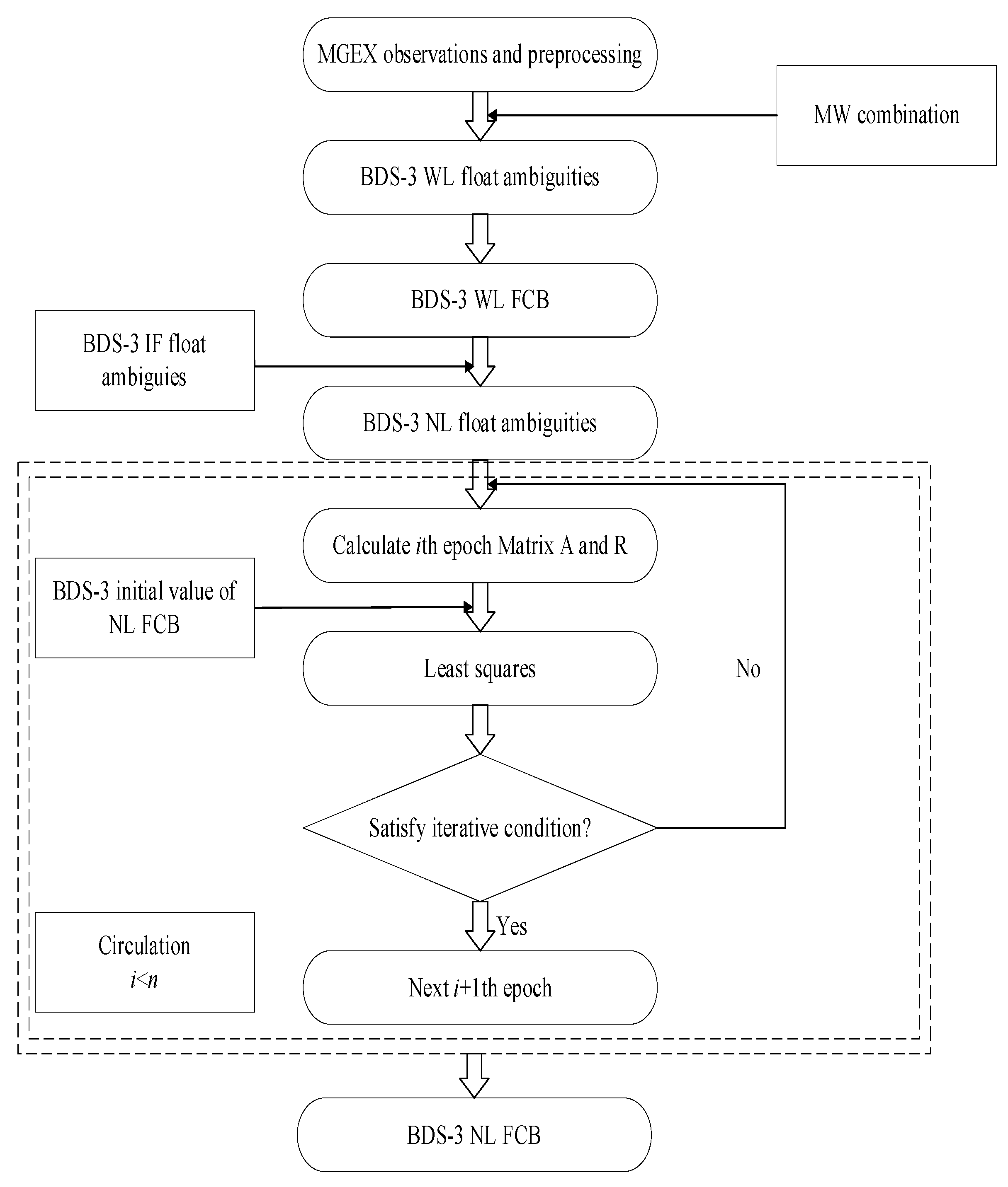
2.2.2. Traditional Estimation of NL FCB

From Equation (10), NL float ambiguity can be expressed as follows:

$${\widehat{N}}_{r,NL}^s=N_{r,1}^s+{\phi }_{r,NL}^{}-{\phi }_{NL}^s$$

(19)

The estimation method of BDS-3 NL FCB is similar to WL FCB; therefore, it can be estimated by Equations (15)–(18). Since the NL float ambiguity is the combination of IF float ambiguity and WL integer ambiguity, the variance of NL FCB is [19]

$${\sigma }_{NL}=\frac{f_1+f_2}{f_1}{\sigma }_{IF}$$

(20)

where ${\sigma }_{IF}$ is the variance of the IF float ambiguity. It can be used to determine the weight of NL FCB by Equation (20). In order to improve the robustness and accuracy of the solution, the IGG3 method can be used for iterative calculation. The following points should be noted when calculating the NL FCB: (1) Due to the short wavelength of NL ambiguity, NL FCB is susceptible to other errors. Thus, the iterative least-squares method is often used to obtain a precise NL FCB, and the initial value of NL FCB can improve the convergent speed of iterative least squares. The method that estimates the initial value of the NL FCB is as follows: First, a station with the largest number of satellite observations is selected as the reference station, and the receiver FCB of the station is set to 0. Then, the satellite FCB of this station can be obtained. For the next station with common-view satellites, the ambiguities of common-view satellites can be corrected by using the FCB of common-view satellites, and these ambiguities should have a close fractional part. The receiver FCB can be obtained by averaging common-view ambiguities. The uncommon-view satellite FCB can be obtained by correcting the receiver FCB in this station. Finally, this method can be used to traverse all stations to obtain all satellite FCB; (2) the NL FCB is unstable in a single day, and therefore, we estimated it every 15 min; (3) it can improve the accuracy of IF float ambiguity by fixed station coordinates in PPP and can improve the accuracy of NL float ambiguity.

Then, the BDS-3 WL and NL FCB can be successfully estimated by using the above method. The specific flowchart of the estimation method is shown in Figure 1.

By analyzing the traditional NL FCB method, we found the following disadvantages: (1) needing an iterative computation when estimating NL FCB—it can consume much time, especially when using many MGEX stations; (2) the reference datum of a traditional initial value of NL FCB was chosen as a receiver FCB at 0. Thus, we had to choose the same reference datum when estimating NL FCB. If not, it could also consume much iterative computation time; (3) the traditional method limited our selection of a reference datum. We could not balance convergence speed and the selection of a reference datum at the same time.

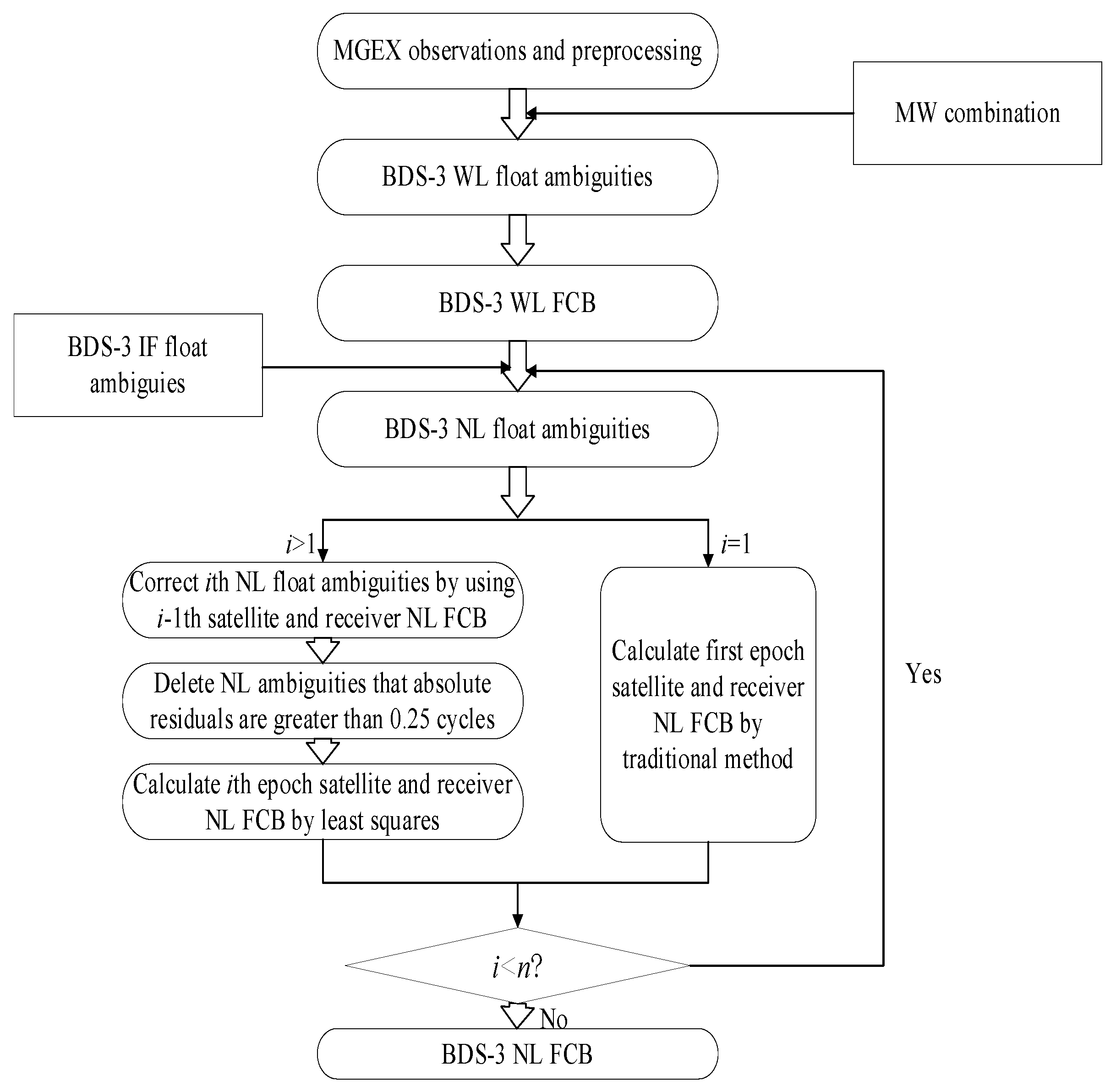
2.2.3. Improved Estimation of NL FCB

As we can see from Section 2.2.2, the traditional estimation of NL FCB needs several iterations and a long time to obtain convergent solutions. In this section, we propose an improved NL FCB method of estimation that does not need any iteration, and we can choose any reference datum. The method can be expressed as follows: (1) we obtained the first epoch satellite and receiver NL FCB by using the method in Figure 1, ${\phi }_{r_1,NL}^{}$ and ${\phi }_{NL}^{s_1}$ representing them, respectively. This may consume some time, but the precision of ${\phi }_{r_1,NL}^{}$ and ${\phi }_{NL}^{s_1}$ is high; (2) for the next epoch, we used ${\phi }_{r_1,NL}^{}$ and ${\phi }_{NL}^{s_1}$ to correct NL float ambiguities first, and these ambiguities should be close to the integer. Then, we eliminated the ambiguities with absolute residuals that are greater than 0.25 cycles. Finally, we obtained precise ${\phi }_{r_2,NL}^{}$ and ${\phi }_{NL}^{s_2}$ by using the least-squares method; (3) similar to step II, we used ${\phi }_{r_2,NL}^{}$ and ${\phi }_{NL}^{s_2}$ to correct the third epoch NL float ambiguities; then, we obtained ${\phi }_{r_3,NL}^{}$ and ${\phi }_{NL}^{s_3}$. Finally, we obtained all epoch satellites and receiver NL FCBs by using this method.

Then, the BDS-3 NL FCB could be successfully estimated by using the proposed method. The specific flowchart of the proposed estimation method is shown in Figure 2.

A comparison of Figure 2 with Figure 1 reveals that the traditional method needs multiple iterations for the initial value of NL FCB, and the iterative condition is that fixed NL ambiguities are not changed. However, before estimating NL FCB, the proposed method deleted NL ambiguities that absolute residuals were greater than 0.25 cycles by using the previous epoch NL FCB. Therefore, the left NL ambiguities are precise, and we could estimate NL FCB by least squares without any iterations. Due to the stable peculiarity of NL FCB of adjacent epochs, we could use this method to correct NL ambiguities. This is the main reason that the proposed method is relatively faster when estimating NL FCB.

3. Results and Discussion

In this paper, in order to analyze the performance of the proposed method, we used the observation data of MGEX station in 2021 to estimate BDS-3 WL and NL FCB. The distribution of MGEX sites is shown in Figure 3.

Since in the first step, we have to establish float ambiguities when estimating NL FCBs, it is necessary to perform PPP calculations for each MGEX station. The data processing model used in PPP in this paper is shown in

Table 1. PPP data processing model.

Processing Type	Correction Model
Satellite orbit error	Precise ephemeris products(CODE,15 min)
Satellite clock error	Precise clock products(CODE, 30 seconds)
Error caused by the rotation of the Earth	Erp products(CODE)
DCB	DCB product(CODE)
Tropospheric delay	Saastamoinen + GPT2w + Estimate
Ionospheric delay	IF model
PCO/PCV	IGS14 atx
Receiver clock error	Estimate
Phase wind-up	Model correction
Solid tide, extreme tide, and ocean tide	Model correction
Elevation mask angle	7
Stochastic model	Elevation model
Parameter estimation method	Kalman filter (constrained station coordinates)

.

3.1. FCB Experiment

As the WL FCB is relatively stable, only one value per day can be estimated. In this paper, we used the MW combination to calculate BDS-3 WL FCB. The time series of WL FCB over the day-of-year (DOY) period of 182–213 are shown in Figure 4.

It can be seen from Figure 4 that the WL FCB of BDS-3 maintains stable characteristics within 30 days. All satellites have a fluctuation range of no more than 0.1 cycles in a single day. The GEO orbit accuracy of BDS-3 is bad, and the WL FCB was not estimated.

The residual error distribution of FCB is also one of the standards for testing the quality of FCB products. In order to analyze the estimation accuracy of the WL FCB, the posteriori residual errors of the WL float ambiguities are shown in the following figures (with 185 days as an example).

The RMS of BDS-3 is 0.098 cycles. The accuracy of WL FCB is high, mainly because of the long wavelength of the WL ambiguity, and not susceptible to various residual errors and observation noise. By analyzing the posteriori residual error figures of Figure 5, it can be seen that the percentages of BDS-3 WL float ambiguity posteriori residual errors are less than 0.15 cycles, which is at 91.73%. Percentages less than 0.25 cycles are at 96.27%. In addition, the residual distribution of BDS-3 is even and symmetrical, and the mean of residual errors is close to 0, which further verifies the precision of the BDS-3 WL FCB.

As evident, the NL float ambiguity can be obtained by using Equation (10) when WL ambiguity is fixed by using the estimated WL FCB. The IF float ambiguity needs to be obtained by PPP before calculating NL float ambiguity. In order to improve the accuracy and stability of IF float ambiguity, we used tight constraints in PPP by using the station coordinates in this paper.

After fixing BDS-3 WL ambiguity by WL FCB, BDS-3 NL float ambiguity is calculated. Then, NL FCB can be estimated by using the proposed method in Section 3.2. The BDS-3 NL FCB for 185 days in 2021 for the traditional and proposed methods is shown in Figure 6 and Figure 7.

We counted the calculated time of the program when estimating NL FCB by different methods. As shown in

Table 2. Hardware configuration details.

Configuration of PC	Details
PC	Lenovo ThinkStation P340
CPU	Intel Core i9-10900 @ 2.80GHz
GPU	NVIDIA Quadro P400
Memory	16G
Mainboard	Lenovo 1048
Hard Disk Drive	256G SSD + 1T HDD

, in the same environment (such as software, computer, number of stations, data, etc.), the calculated time of the traditional method is 27386 seconds, and the calculated time of the proposed method is 17881 seconds. The calculated time is the average time over 10 runs. Therefore, the computational efficiency of NL FCB increases by about 34.71% when using the proposed method. Figure 6b and Figure 7b show 1–10 epochs of NL FCB by the traditional and proposed methods, which are also included in the overall epochs in one day, shown in Figure 6a and Figure 7a. We can see that the NL FCB of the traditional method needs about four epochs to be stable. From Figure 7b, the NL FCB of the proposed method is more stable in 1–10 epochs.

The residual errors distribution of FCB is also one of the standards for testing the quality of FCB products. For analyzing the estimation accuracy of NL FCB, the posteriori residual errors of the NL float ambiguities are shown in Figure 8.

The RMS of posteriori residual errors with the traditional and proposed methods are 0.0928 and 0.087 cycles, respectively. The accuracy of NL FCB is high, mainly because IF ambiguity is relatively stable after fixing the coordinates in PPP. While analyzing the posteriori residuals shown in Figure 8, when using the traditional method, 88.19% of residuals are less than 0.15 cycles and 99.99% of residuals are less than 0.25 cycles. When using the proposed method, 88.43% of residuals are less than 0.15 cycles, and 99.99% of residuals are less than 0.25 cycles. This shows that the precision of NL FCB is close with each method. In addition, the residual distribution of BDS-3 is even and symmetrical, and the mean residual error is close to 0, which further verifies the precision of the BDS-3 NL FCB when using different methods.

3.2. PPP–AR Experiment

In order to analyze the performance of FCB, estimated by the proposed method, we carried out some static and dynamic PPP–AR experiments by using the data of European reference stations and comparing them with the traditional method. The European reference stations are distributed, as shown in Figure 9.

In the static PPP–AR experiments, we used two indexes to assess the performance of FCB products, which are

$$\eta =\frac{n_{epoch,fixed}}{N_{epoch,all}}$$

(21)

$$\xi =\frac{n_{amb,fixed}}{N_{amb,all}}$$

(22)

where $\eta$ is the rate of the fixed epoch, $n_{epoch,fixed}$ is the number of the fixed epoch, and $N_{epoch,all}$ is the number of all epochs in a station. $\xi$ is the rate of fixed ambiguities, $n_{amb,fixed}$ is fixed NL or WL ambiguities, and $N_{amb,all}$ is all NL or WL ambiguities in a station.

To verify the suitability of the FCB products estimated by the proposed method for positioning, BDS-3 data from 37 European reference stations were selected on day 185. As WL FCBs are estimated in a similar way in both the traditional and the proposed method, we only calculated ${\eta }_{static}$ and ${\xi }_{static,NL}$ in this paper. The results of static PPP–AR by using different methods are shown in Figure 10 and Figure 11.

From Figure 10, the ${\eta }_{static}$ of most stations is more than 90%, and the mean ${\eta }_{static}$ that uses the traditional and proposed methods are 94.50% and 94.96%, respectively. The ${\eta }_{static}$ of the proposed method is 0.5% more than in the traditional method. From Figure 11, the ${\xi }_{static,NL}$ values using the traditional and proposed methods are 77.61% and 78.03%, respectively. The mean ${\xi }_{static,NL}$ of the proposed method is 0.5% more than in the traditional method. Therefore, the proposed method offers an improved precision compared to the traditional one. We also counted the time to first fixed (TTFF) of the stations, and the results are shown in Figure 12.

We believe the ambiguities would be fixed steadily if the ambiguities are fixed for 10 min in the PPP–AR experiments. From Figure 12, we can deduce that the TTFF of the proposed method is shorter than in the traditional method. The mean TTFF of the traditional and proposed methods are 35.56 and 28.56 min, respectively. The mean TTFF decreased by 19.69% when employing the proposed method.

To further analyze the performance of the FCB obtained by the proposed method, we also carried out PPP–AR experiments in the dynamic model. Using the same observations, we set the processing noise of the coordinate estimation as white noise with a variance of 10⁶ m² for PPP in dynamic mode, and the results are shown in Figure 13 and Figure 14.

From Figure 13, it can be inferred that the mean ${\eta }_{dynamic}$ values that are used in the traditional and proposed methods are 93.51% and 94.15%, respectively. The ${\eta }_{dynamic}$ of the proposed method is 0.7% more than the traditional method in the dynamic model. The results shown in Figure 14 indicate that the mean ${\xi }_{dynamic,NL}$ values using the traditional and proposed methods are 77.34% and 77.86%, respectively. The mean ${\xi }_{dynamic,NL}$ of the proposed method is 0.5% more than the traditional method. Compared with the static model, the $\eta$ of the traditional and proposed methods is less than 0.99% and 0.81%, respectively, and the ${\xi }_{NL}$ of the traditional and proposed methods is less than 0.27% and 0.17%, respectively, due to the influence of noise.

Compared with the static model, the TTFF of stations in the dynamic model is larger. From Figure 15, it is evident that the mean TTFF of the traditional and proposed methods is 42.35 and 30.14 min, respectively. The mean TTFF decreased by 28.83% when employing the proposed method. The results show that the FCB of the proposed method has better suitability and precision.

3.3. Discussion

Compared with the results of [20], the rate of fixed epoch and TTFF when using the traditional method in this paper increased by 4% and 10 min. The main reasons for this are the number of BDS-3 satellites and because the precision of the final products of BDS-3 increased. The accuracy of orbit and clock products is the most effective factor for the estimation of NL FCB. As the number of stations that can observe BDS-3 satellites increase, the accuracy of BDS-3 final products will be better, and the accuracy of NL FCB is expected to be further improved.

The rate of fixed NL ambiguities is only 78% in this paper, although the rate of the fixed epoch is more than 90%. The accuracy of BDS-3 orbit and clock products is one of the important reasons for this rate; another reason may be the lower rate of fixed WL ambiguities. The rate of fixed WL ambiguities is shown in Figure 16.

We did not address the rate of fixed WL ambiguities in the experiment due to the same method when estimating WL FCB. Figure 16 depicts that the mean rate of fixed WL ambiguities is 90.17%. In this paper, we estimated FCB by using the B1I/B3I signal of BDS-3. It is expected to further improve the rate of fixed WL ambiguities by using the B1C/B2A signal of BDS-3, due to the new signal having more precise observations [19]. It can also improve the rate of fixed NL ambiguities and the reliability of PPP–AR.

4. Conclusions

The traditional method needs multiple iterations when estimating satellite phase NL fractional cycle biases. Although the initial value can decrease the time of iterations, it also needs some time to obtain convergent solutions. The traditional initial value is equivalent to setting a receiver FCB to zero when selecting the reference of NL FCB. If the same reference is not selected, it can also increase the time of iterations. In this paper, we proposed an improved fast estimation of FCB, which did not need any iterations. The proposed method can estimate FCB quickly and precisely, and we verified this method in the BDS-3 experiments.

In the FCB experiments, the results showed that the two methods have the same accuracy of estimation of NL FCB. However, the calculated time of the proposed method was less than the traditional method, and the computation efficiency increased by 34.71%. In the PPP–AR experiments, the rate of the fixed epoch and ambiguities with the static model by the proposed method increased by 0.5%, and the TTFF of the proposed method in the static model decreased by 19.69%. The rate of the fixed epoch and ambiguities in the dynamic model using the proposed method increased by 0.7% and 0.5%, respectively, and the TTFF of the proposed method in the dynamic model decreased by 28.83%. This shows that the proposed method has a better convergence time in PPP–AR.

Compared with the traditional method, the improved fast estimation of FCB is more suitable in the estimation of real-time FCB, and it can estimate real-time FCB more quickly and precisely.

References

1. Zumberge, J.; Heflin, M.; Jefferson, D.; Watkins, M.; Webb, F. Precise point positioning for the efficient and robust analysis of GPS data from large networks. J. Geophys. Res. Solid Earth 1997, 102, 5005–5017. [Google Scholar] [CrossRef] [Green Version]
2. Héroux, P.; Kouba, J. GPS precise point positioning using IGS orbit products. Phys. Chem. Earth Part A Solid Earth Geod. 2001, 26, 573–578. [Google Scholar] [CrossRef]
3. Ye, S. Theory and Realization of GPS Precise Point Positioning Using Un-Differenced Phase Observation. Ph.D. Thesis, Wuhan University, Wuhan, China, 2002. [Google Scholar]
4. Gao, Y.; Shen, X. Improving Ambiguity Convergence in Carrier Phase-Based Precise Point Positioning. In Proceedings of the 14th International Technical Meeting of the Satellite Division of the Institute of Navigation (ION GPS 2001), Salt Lake City, UT, USA, 11–14 September 2001; pp. 1532–1539. [Google Scholar]
5. Cai, C.; Gao, Y. Performance analysis of Precise Point Positioning based on combined GPS and GLONASS. In Proceedings of the 20th International Technical Meeting of the Satellite Division of the Institute of Navigation (ION GNSS 2007), Fort Worth, TX, USA, 25–28 September 2007; pp. 858–865. [Google Scholar]
6. Cai, C.; Gao, Y. Precise point positioning using combined GPS and GLONASS observations. Positioning 2007, 1, 13–22. [Google Scholar] [CrossRef] [Green Version]
7. Cai, C.; Gao, Y. Modeling and assessment of combined GPS/GLONASS precise point positioning. GPS Solut. 2013, 17, 223–236. [Google Scholar] [CrossRef]
8. Martín, A.; Anquela, A.; Capilla, R.; Berné, J. PPP technique analysis based on time convergence, repeatability, IGS products, different software processing, and GPS+ GLONASS constellation. J. Surv. Eng. 2011, 137, 99–108. [Google Scholar] [CrossRef]
9. Li, P.; Zhang, X. Integrating GPS and GLONASS to accelerate convergence and initialization times of precise point positioning. GPS Solut. 2014, 18, 461–471. [Google Scholar] [CrossRef]
10. Montenbruck, O.; Steigenberger, P.; Khachikyan, R.; Weber, G.; Langley, R.; Mervart, L.; Hugentobler, U. IGS-MGEX: Preparing the ground for multi-constellation GNSS science. Inside Gnss 2014, 9, 42–49. [Google Scholar]
11. Xiaohong, Z.; Xingxing, L.; Pan, L. Review of GNSS PPP and its application. Acta Geod. Cartogr. Sin. 2017, 46, 1399. [Google Scholar] [CrossRef]
12. Gabor, M.J.; Nerem, R.S. GPS Carrier Phase Ambiguity Resolution Using Satellite-Satellite Single Differences. In Proceedings of the 12th International Technical Meeting of the Satellite Division of The Institute of Navigation (ION GPS 1999), Nashville, TN, USA, 14–17 September 1999; pp. 1569–1578. [Google Scholar]
13. Ge, M.; Gendt, G.; Rothacher, M.A.; Shi, C.; Liu, J. Resolution of GPS carrier-phase ambiguities in precise point positioning (PPP) with daily observations. J. Geod. 2008, 82, 389–399. [Google Scholar] [CrossRef]
14. Zhang, X.; Li, P.; Guo, F. Ambiguity resolution in precise point positioning with hourly data for global single receiver. Adv. Space Res. 2013, 51, 153–161. [Google Scholar] [CrossRef]
15. Laurichesse, D.; Mercier, F.; Berthias, J.P.; Broca, P.; Cerri, L. Integer ambiguity resolution on undifferenced GPS phase measurements and its application to PPP and satellite precise orbit determination. Navigation 2009, 56, 135–149. [Google Scholar] [CrossRef]
16. Collins, P.; Bisnath, S.; Lahaye, F.; Héroux, P. Undifferenced GPS ambiguity resolution using the decoupled clock model and ambiguity datum fixing. NAVIGATION J. Inst. Navig. 2010, 57, 123–135. [Google Scholar] [CrossRef] [Green Version]
17. Geng, J.; Meng, X.; Dodson, A.H.; Teferle, F.N. Integer ambiguity resolution in precise point positioning: Method comparison. J. Geod. 2010, 84, 569–581. [Google Scholar] [CrossRef] [Green Version]
18. Shi, J.; Gao, Y. A comparison of three PPP integer ambiguity resolution methods. GPS Solut. 2014, 18, 519–528. [Google Scholar] [CrossRef]
19. Li, R.; Wang, N.; Li, Z.; Zhang, Y.; Wang, Z.; Ma, H. Precise orbit determination of BDS-3 satellites using B1C and B2a dual-frequency measurements. GPS Solut. 2021, 25, 95. [Google Scholar] [CrossRef]
20. Li, X.; Li, X.; Liu, G.; Yuan, Y.; Zhou, F. BDS multi-frequency PPP ambiguity resolution with new B2a/B2b/B2a + b signals and legacy B1I/B3I signals. J. Geod. 2020, 94, 107. [Google Scholar] [CrossRef]
21. Liang, Z.; Yang, H.; Yang, G.; Yao, Y.; Xu, C. Evaluation and analysis of real-time precise orbits and clocks products from different IGS analysis centers. Adv. Space Res. 2018, 61, 2942–2954. [Google Scholar] [CrossRef]
22. Kouba, J. A Guide to Using International GNSS Service (IGS) Products. 2009. Available online: https://kb.igs.org/hc/en-us/articles/201271873-A-Guide-to-Using-the-IGS-Products (accessed on 14 October 2021).
23. Hatch, R. The Synergism of GPS Code and Carrier Measurements. In Proceedings of the International Geodetic Symposium on Satellite Doppler Positioning, Las Cruces, NM, USA, 8–12 February 1982; pp. 1213–1231. [Google Scholar]
24. Melbourne, W.G. The Case for Ranging in GPS-Based Geodetic Systems. In Proceedings of the First International Symposium on Precise Positioning with the Global Positioning System, Rockville, MD, USA, 15–19 April 1985; pp. 373–386. [Google Scholar]
Figure 1. Flowchart of the traditional BDS-3 FCB method of estimation.
Remotesensing 14 00334 g001
Figure 2. The flowchart of improved BDS-3 FCB method of estimation.
Remotesensing 14 00334 g002
Figure 3. Distribution of MGEX sites.
Remotesensing 14 00334 g003
Figure 4. BDS-3 WL FCB (reference satellite is C19).
Remotesensing 14 00334 g004
Figure 5. BDS-3 WL float ambiguity posteriori residual errors distribution (2021, day 185).
Remotesensing 14 00334 g005
Figure 6. NL FCB of BDS-3 estimated by using the traditional method (reference satellite is C19) as (a) NL FCB of all epochs in one day; (b) NL FCB of 1–10 epochs in one day.
Remotesensing 14 00334 g006
Figure 7. NL FCB of BDS-3 estimated by using the improved fast method (reference satellite is C19) as (a) NL FCB of all epochs in one day; (b) NL FCB of 1–10 epochs in one day.
Remotesensing 14 00334 g007
Figure 8. Distribution of float posteriori NL ambiguity residual errors (2021, day 185) as (a) posteriori residual errors when estimating NL FCB with traditional method; (b) posteriori residual errors when estimating NL FCB with proposed method.
Remotesensing 14 00334 g008
Figure 9. Distribution of European reference stations.
Remotesensing 14 00334 g009
Figure 10. Rate of fixed epochs by using different bias products (2021, day 185).
Remotesensing 14 00334 g010
Figure 11. Rate of fixed NL ambiguities by using different bias products (2021, day 185).
Remotesensing 14 00334 g011
Figure 12. TTFF of 37 stations by static model.
Remotesensing 14 00334 g012
Figure 13. Rate of fixed epoch by using different methods in the dynamic model.
Remotesensing 14 00334 g013
Figure 14. Rate of fixed NL ambiguities by using different methods in the dynamic model.
Remotesensing 14 00334 g014
Figure 15. TTFF of 37 stations in the dynamic model.
Remotesensing 14 00334 g015
Figure 16. Rate of fixed WL ambiguities by using the two different methods.
Remotesensing 14 00334 g016