Abstract
This study based on co-occurrence analysis shearlet transform (CAST) effectively combines the latent low rank representation (LatLRR) and the regularization of zero-crossing counting in differences to fuse the heterogeneous images. First, the source images are decomposed by CAST method into base-layer and detail-layer sub-images. Secondly, for the base-layer components with larger-scale intensity variation, the LatLRR, is a valid method to extract the salient information from image sources, and can be applied to generate saliency map to implement the weighted fusion of base-layer images adaptively. Meanwhile, the regularization term of zero crossings in differences, which is a classic method of optimization, is designed as the regularization term to construct the fusion of detail-layer images. By this method, the gradient information concealed in the source images can be extracted as much as possible, then the fusion image owns more abundant edge information. Compared with other state-of-the-art algorithms on publicly available datasets, the quantitative and qualitative analysis of experimental results demonstrate that the proposed method outperformed in enhancing the contrast and achieving close fusion result.
1. Introduction
Image fusion, as a main part of the image enhancement technology, aims to assimilate the abundant and valid detail information of the heterogeneous source images to construct a fused image with rich and interesting information [1,2,3,4]. Moreover, for the image fusion of multi-sensor, the research on the fusion of infrared and visible images is more common [5]. The fused image with robustness and rich information about the scene is significant for a lot of applications such as surveillance, remote sensing, human perception and computer vision tasks [6], etc. Although visible images possess texture details in high resolution, under poor conditions such as low illumination, smoke and occlusion, the quality of the visual images is hardly satisfying, and some important target information will be lost [7]. However, the infrared sensors generate an image via capturing the heat radiation from the object and the salient information of the target in the complicated scene can be actively obtained. Therefore, the infrared images usually are selected as the offset for visual image during above bad environment. Via combining the complementary sources of information effectively from these two kinds of images in the same scene, the disadvantages of the human eyes’ visual characteristics can be improved, and the range of the human visual band can be extended greatly [2,8].
Multi-scale transform (MST), as the most general method, is adopted in image fusion applications by numerous researchers with visual fidelity, lower computational complexity and higher efficiency [3,9]. Generally speaking, the fusion method based on the MST consists of 3 stages. First and foremost, the original image data is decomposed into multi-scale transform domain. Secondly, sub-coefficients in each scale are constructed by the specific fusion algorithm. Finally, the fused image is obtained by a relevant inverse transform [9]. At present, the MST algorithms primarily include Laplacian pyramid (LP) [10], wavelet transform (WT) [11], non-subsampled contourlet transform (NSCT) [12], and non-subsampled shearlet transform (NSST) [13]. Moreover, the MST methods are not sensitive enough to edge details, and the fused image is easy to smooth much more detail information during reconstruction.
Lately, more and more scholars applied the edge-preserving filtering (EPF) to the fields of image processing [9,14,15]. The edge details of the source images can be preserved as many as possible and the images can also be smoothed well. The universal EPF methods include Gaussian curvature filtering (GCF) [16], bilateral filtering (BF) [17], guided filtering (GF) [18,19] and rolling guidance filter [20]. Supposing EPF is also used as an image decomposition method, the results are full of more spatial information, and various components compared with MST methods. These traditional edge-preserving filters are dedicated to smoothing the edges of the images. However, they cannot completely distinguish between the edges in the texture area and the boundaries among the texture areas. Jevnisek et al. put forward co-occurrence filter (CoF), which performs on the pixel itself via the data statistics of the co-occurrence information in the original image [21]. Therefore, CoF is excellent enough in smoothing the edge details in the texture area and retaining the borderlines through the texture area. In this paper, a novel decomposition method based on co-occurrence analysis shearlet transform is proposed, which is introduced in Section 2.
On account of the low-rank representation (LRR), Latent low-rank representation (LatLRR) [22] is proposed, which can effectively analyze the multiple subspaces of data structures. From another perspective, the original image mainly contains base components, salient components, and some sparse noise according to the decomposition based on LatLRR [23]. In addition, the salient components that represent the space distribution of saliency information can be separated from the source images based on LatLRR [24]. Then, the saliency map formed by LatLRR algorithm is usually selected as the fusion rule to construct the fused image from heterogeneous images for base-layer images. The fusion rule is an effective method in which the weight value can be assigned adaptively according to the salient information.
For detail-layer sub-images, the common ‘‘max-absolute” method usually is adopted as the fusion rule, in which highly salient texture features correspond to large absolute values, but some redundant information of the original images can be easily abandoned by this rule. This paper chose the number of zero crossings in differences [25] as the regularization term to assist the fusion of the detail-layer images. In addition, the texture gradient features can be transferred to the fused image of the detail-layer as much as possible via this method. The model uses the counting measure regularization to weaken low-contrast intensity changes and keep drastic gradients.
In view of the review above, this paper puts forward a novel fusion framework based on the weight map of LatLRR and the regularization term of zero-crossing counting for visual and infrared images. Above all, the CAST is utilized as the MST method, in which the infrared and visual images can be decomposed finely. Next, the base-layer and detail-layer components can be fused via their respective fusion rules, namely the saliency information guiding map based on LatLRR and the counting zero-crossing regularization [26]. Finally, the fused sub-images are reconstructed by corresponding inverse transform.
The rest of the paper is arranged as follows. The fundamental theory of the CAST, LatLRR and Counting the Zero crossings in differences are introduced in Section 2. The novel fusion framework is proposed and shown in Section 3. The Section 4 is the part about experimental setting and result analysis. The conclusion of this algorithm is expounded in Section 5.
2. Related Work
In this section, for a comprehensive review of some algorithms most relevant to this study, we focus on reviewing including co-occurrence filter, directional localization, latent low rank representation, and counting the zero crossings in differences.
2.1. Co-Occurrence Filter
The co-occurrence filter (COF) [27] assigns the weight value in accordance with the co-occurrence information, so that the weight of the frequently occurring texture information is reduced and smoothed, and the weight of the infrequently occurring edge information is increased. In this way, the idea of edge detection is directly applied to the filtering process. It is the perfect combination of edge detection and edge preservation. Figure 1 shows the comparison between before and after co-occurrence filter processing.
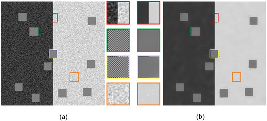
Figure 1.
Working principle of Co-occurrence filter. (a) Image before COF processing, (b) Image after COF processing.
Based on the Bilateral Filter, the COF introduces the normalized co-occurrence matrix to take the place of the range Gaussian [4,16]. In addition, the definition of the COF is as follows:
where and denote the output and input pixel value, respectively, and , are pixel indexes; represents the weighted item, measuring the contribution of pixel to output pixel , is the Gaussian filter, is 256 × 256 matrix for general gray-scale images computed from the following formula:
where is called as the co-occurrence matrix, and used to collect the co-occurrence information of the original images; and denote the histogram of pixel values corresponding to frequency statistics of the pixel and [28]. The co-occurrence matrix can be obtained by the following formulas:
where means the parameter of the COF which can control the filtering of the edge texture in the image and is usually 15; the symbol represents a value definition relationship: if the Boolean expression in the bracket is true, its value is 1, otherwise the value is 0; represents the Euclidean distance from pixel to in the image plane.
Thence, the COF has excellent performance in smoothing the edges within the texture area and preserving the boundaries across the texture area. It is obvious that Gaussian white noise and checkerboard textures are common in the figure, so that the co-occurrence matrix gives them higher weight. On the contrary, because the borders of dark and shallow areas appear less frequently, they are given a relatively low weight. COF can remove noise and smooth texture areas, while clearly retaining the boundaries between different texture areas. Given the edge retention filter does not blur the edge when decomposing the image, and there is no ringing effect and artifacts, then there is a good spatial consistency and edge retention [21].
2.2. Directional Localization
In view of the advantages of the local shearlet filter, such as removing the block effect, attenuating the Gibbs phenomenon, and improving the convolution calculation efficiency in time domain, it is applied to processing the high-frequency images to realize the directional localization [29]. The decomposition framework is shown in Figure 2.
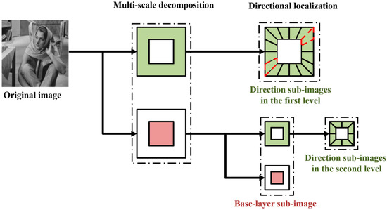
Figure 2.
Image decomposition framework of the proposed method.
The detail-layer image decomposition process is as follows:
- (1)
- Coordinate mapping: from the pseudo-polar coordinates to the Cartesian coordinates;
- (2)
- Based on the “Meyer” equation, construct the small-size shearlet filter;
- (3)
- The k band-pass detail-layer images and the “Meyer” equation are processed by convolution operation [26].
2.3. Latent Low Rank Representation
Visual saliency detection applies certain intelligent processing algorithms to simulate the bionic mechanism of human vision, and analyze the salient targets and areas in a scene. The saliency map consists of the weight information about the image gray value [30]. In this way, the higher the gray value, the greater its saliency, and the larger weight value is allocated during image fusion. In view of the above, more and more scholars use saliency detection on the image fusion field. For example, the latent low rank representation (LatLRR) is commonly used in extracting salient features from the original image data [22].
The LatLRR problem can be solved by minimizing the following optimization function:
where denotes the data matrix of original image, is a low-rank component matrix, denotes the projection matrix of saliency component, and represents a sparse matrix with noisy [5]; is a regularization term, which is usually chosen by cross-validation; is the nuclear norm and denotes ℓ1-norm.
The projection matrix can be obtained by LatLRR method, and the saliency parts of the original image can be calculated by the projection matrix. The result of LatLRR method is shown as the Figure 3. Firstly, select a window. Then, in the horizontal and vertical direction, move the window by the S pixels at each stride. Moreover, via sliding the window, the original image can be partitioned into a lot of image patches. Finally, a new matrix can be acquired, in which all the image patches are reshuffled and every column corresponds with an image patch [5]. In Equation (6), the saliency part () is solved via the projection matrix , the preprocessing matrix and the source data .
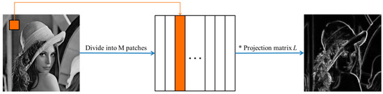
Figure 3.
The process of image saliency features extracting based on LatLRR method.
The result of decomposition is defined as , and the function of contains the window sliding, image partition and reshuffling technique. denotes the reconstruction of the saliency image from the detail part. As recovering , the overlapped pixels are processed by the averaging strategy, in which the pixel average value is calculated via counting the number of the overlapped pixels in the recovered image.
2.4. Counting the Zero Crossings in Difference
The number of zero crossings, which is a gradient-aware statistic method, can ensure that the similarity between the processed signal and the original signal is higher. In addition, there are fewer intervals at each of which it is monotonous, either increased or decreased, convex or concave in the processed signal. In this paper, the optimization problem about the number of zero crossings can be solved by evaluating the proximity operator [25].
2.4.1. Proximity Operator of the Number of Zero Crossings
Zero crossing means that the signal passes through the zero point, and the frequency of the signal fluctuations can be measured by this method. The number of zero crossings is defined as follows:
Suppose is a partition of the vector () into sub-vectors according to the following conditions:
- (1)
- The number of non-zero elements in each segment is one at least.
- (2)
- None-zero elements’ signs in the same segment are the same.
- (3)
- None-zero elements’ signs in adjacent segments are opposite.
Provided the k-th segment can be denoted as , the partition () is called the Minimum Same Sign Partition [31] (MSSP for abbreviation).
Therefore, the number of zero crossings of the vector can be defined as:
Next, we need to consider the problem of minimizing the proximity operator of , and introduce auxiliary variable :
Denote the loss function that needs to be minimized as , namely:
In order to minimize the value of , there are only two possibilities for the value of every element in the optimal solution, that is or . It should be pointed out that the symbol 0 here represents a zero vector [32].
Take to represent the loss function of part of the data , and is an optimal solution vector of the problem (9). Rewriting, the Formula (9) becomes:
Consider the constrained minimum loss function of the last segment
The optimal solution vector (, ) of the Formula (10) must meet the solution vector that or can take the minimum value. In addition, it is obvious that both and will not be 0 at the same time, so there are only two possible situations: (1) ; (2) and . Using , then for , the problem can be written as
Algorithm 1 summarizes the process of using dynamic programming to solve Equation (8), using the form of filling from the bottom up.
| Algorithm 1. Evaluating the proximity operator of |
| Input: Vector , smoothing parameter λ, weight parameter β. |
| Output: The result u, namely is the proximity operator of . |
| 1 Find a MSSP from vector g. |
| 2 Initialize relative parameter . |
| 3 Calculate e, then we can get and . |
| 4 If M ≥ 2 then |
| 5 For j = 3 to M |
| 6 solve for in Equation (11) to compute the minimum loss. |
| 7 End for |
| 8 Update the parameter j ← M + 1 |
| 9 While j ≥ 2 do |
| 10 |
| 11 |
| 12 End while |
| 13 End if |
2.4.2. Image Smoothing with Zero-Crossing Count Regularization
In order to smooth the image of the detail layer, the horizontal and vertical differences of the image S are processed with regularization:
where denotes the ℓ2-norm; is the input image, and is the number of rows and columns of the image ; or (first-order difference or second-order difference) [33,34], and represent the horizontal and vertical difference operators, respectively; () is a relatively important value that can balance the data items and the regularization items. Next, the problem (13) can be solved via using the alternating direction method of multipliers [35] (ADMM) algorithm.
First, the auxiliary variables and are introduced instead of and , respectively, and the Formula (13) becomes
Then its Lagrangian augmented matrix is:
where and are the iterative variables of and , and their values they take can be updated by Equation (19).
The ADMM framework consists of the following iterative formulas:
In the Equation (16), in order to calculate separately each column of the vector , each column of the vector should be decoupled with the others, which allow us to solve each column separately. The Equation (16) can be rewritten as
Likewise, the Equation (17) takes the simple form
where is the weight parameter, which will gradually increase after each iteration. Equations (20) and (21) can be solved efficiently by dynamic programming [36,37,38].
Algorithm 2 summarizes the zero-crossing smoothing algorithm, in which the update of auxiliary variables and needs to rely on Algorithm 1: Our algorithm is sketched in Algorithm 2.
| Algorithm 2. Image smoothing via counting zero crossings |
| Input: Source image I, smoothing weight λ, parameters β, and rate k. |
| Output: Processed image S. |
| 1 Initialization: , . |
| 2 Calculate the vertical difference V via Equation (20) based on Algorithm 1. |
| 3 Calculate the horizontal difference H via Equation(21) based on Algorithm 1. |
| 4 Repeat |
| 5 Calculate S by Equation(18). |
| 6 Calculate and by Equation(19). |
| 7 Update the weight parameter . |
| 8 Until stop condition: the weight parameter . |
| 9 End |
3. The Proposed Method
The overall fusion framework of the proposed algorithm is shown in Figure 4, mainly including three parts, which are image decomposition, sub-images fusion, and the final image reconstruction.
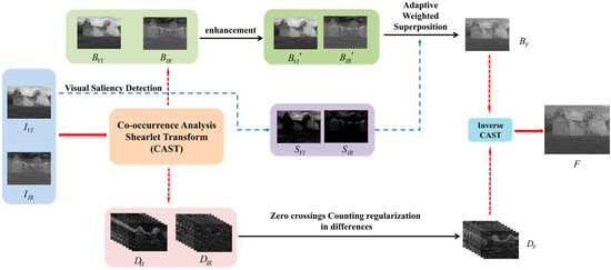
Figure 4.
Image fusion framework based on the proposed method.
3.1. Image Decomposition by CAST
Co-occurrence analysis shearlet transform (CAST), a novel hybrid multi-scale transformation tool, combines the advantages of co-occurrence filter (COF) and shearlet transform. In addition, the filter process is as following.
3.1.1. The Multi-Scale Decomposition Steps of COF
and denote the original visual image and infrared image, and are the corresponding base layer images, and COF is applied to scale the source images:
The detail layer images are obtained by calculating the difference between the original image and the base image, and described as and , respectively.
Then the K-scale decomposition is in the form,
3.1.2. Multi-Directional Decomposition by Using Discrete Tight Support Shearlet Transform
In fact, the traditional shearlet transform is qualified enough for this step. In addition, on this basis, parabolic scaling function is adopted to control the size of the shear filter within a reasonable range. In addition, according to the support range of the shearlet function, the relationship between and can be given qualitatively. Thus, an adaptive multi-directional shearlet filter is constructed as following:
where the parameters and denote the sizes of the input image, represents the multi-directional decomposition scale parameter, and is the size of shear filter.
The adaptive shear filter used in this paper performs multi-directional shearlet transformation on each scale detail layer, so as to effectively obtain the optimal multi-directional detail components. The decomposition details are shown in Figure 5.
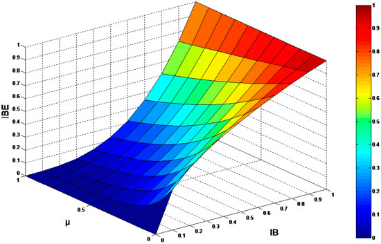
Figure 5.
Diagram of Brightness Correction Function.
3.2. The Brightness Correction of Based-Layer Image
The grey-scale image is more in line with human visual requirements, if its gray value ranges between 0 and 1, and the average value of the image is 0.5. In fact, it is not possible that every image is optimal. As a result, the omega correction can be introduced to revise the brightness of the base layer [39].
The definition of the omega correction is as follows:
where presents the base component of the input image; denotes the base component corrected by the correction parameter , and the extension degree of the image can be controlled via the parameter . Obviously, when , the corrected image is the same as the input image absolutely; when , the corrected image is a bit brighter, and the overall brightness of will increase with the decrease of the parameter omega; on the contrary, when , the corrected image becomes darker than the input image. In addition, the parameter omega can be derived from the following formula:
where is the rate of correction, and denotes the average gray value of the base layer image in the window. Figure 5 indicates that the lower the value of is, the higher the pixel enhancement level is. If is less than 0.5, the image of the window seems dark, and the value of the image will be corrected via the brightness correction function and vice versa.
3.3. Fusion Rule of Base-Layer Image
The base components of the original images consist of the fundamental structures, the redundant information and light intensity, which are the approximate parts and the main energy parts. In fact, the effect of the final fused image is dependent on the fusion rule of the base layer. In order to improve the brightness of the visual image, the omega correction function and the saliency information weighted map are utilized to fuse the base layer components.
For the sake of preventing incompatible spectral characteristics from heterologous images, LatLRR, is utilized to generate the weighted map to guide the fusion of the base-layer images adaptively. The specific fusion strategy of the base components is provided below:
Step 1: The saliency features of visual and infrared images can be calculated by the LatLRR algorithm. The corresponding weighted maps and are constructed. In addition, the normalized weighting coefficient matrices of and can be obtained by the salient maps’ values.
Step 2: The parameters of and are applied to implement weighted fusion of the base-layer images adaptively. The specific formulas are as follows:
where and are defined as the weights of the base layers, and are the base layer images of visual and infrared images, respectively, and denotes the final base-layer fused coefficients.
Considering the spectral differences between the two original images, it can be compensated by the weighted map. At the same time, the contrast of the visual images can be improved. In addition, the weighted map mainly is the weighting distribution of the grayscale value in space, and this fusion strategy can adaptively transfer the saliency components of the infrared images to the visual images with textural components as many as possible. Finally, the fusion effect of the base-layer images can be greatly improved by the appropriate combination of the salient components between the two original images [24].
3.4. Fusion Rule of Detail-Layer Image
In contrast with the base-layer images, the detail layers of the images preserve more structural information, such as some edge and texture components. So the fusion strategy of the detail-layer components can also affect the final visual effect of the fused image. In order to avoid excessive punishment for adjacent pixels with large intensity differences, the number of zero crossings in differences is selected as the regularization term to penalize the number of convex or concave segments of the sub-images.
The fusion strategy based on mixed zero-crossing regularization is put forward, the expression of which can be described as follows:
where , and denote the detail-layer sub-coefficients of visual image, infrared image, and fused image, respectively; is the number of the decomposition, represents the decomposition direction in each layer, and are the regularization coefficients, represents the ℓ2-norm, indicates the counting zero crossings and is the second-order difference operator. Furthermore, the gradient parameter can be used to weigh the importance of two types of detail-layer components in spatial distribution. The expression of is shown as follows:
When , namely , the detail-layer coefficients of the visual image domain the main features of the fusion image, and the zero-crossing number of the detail-layer coefficients in infrared image is selected as the regular term for supplement. On the contrary, indicates that the detail layer sub-coefficients of the infrared image include more information.
Next, using ADMM algorithm to solve the problem (36), the process is as follows:
Step 1: Let the parameters and replace and operators, respectively, so the Equation (36) becomes:
Step 2: When , the Lagrangian augmented function is:
Step 3: The ADMM framework consists of the following iterative formulas:
where is the weight parameter, which will gradually increase after each iteration until satisfies the termination criterion of the iteration. In addition, Equations (40) to (43) can be solved efficiently by dynamic programming.
When , repeat the step 2 and step 3. By repeating the above steps, the fused images of the detail layers can be obtained. This final fusion effect will be tested in the experiments of the Section 4.
4. Experimental Results and Analysis
So as to affirm the fusion effect of the proposed method in this paper, the common infrared and visual image fusion sets are used as experimental data. Moreover, some classic and state-of-the-art algorithms are tested to compare with our algorithm from qualitative and quantitative aspects, respectively.
4.1. Experimental Settings
Seven pairs of infrared and visible images (i.e., namely, Road, Camp, Car, Marne, Umbrella, Kaptein and Octec) from TNO [40] are selected for testing, which are exhibited in Figure 6.
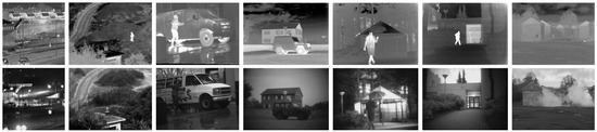
Figure 6.
Seven pairs of input images. The first row consists of infrared images, and the bottom row contains visual images. From left to right are Road, Camp, Car, Marne, Umbrella, Kaptein and Octec.
Among them, “Road” is a set of images taken under the low illumination condition. The image pair of “Camp” contains rich background information in the visible image and has the clearer hot targets in another image. Both visible and infrared images in “Car”, “Marne”, “Umbrella” and “Kaptein” contain significant and abundant information. In “Octec”, the infrared image has the interesting region, but the visible image is blocked by smoke. The size of images is 256 × 256, 270 × 360, 490 × 656, 450 × 620, 450 × 620, 450 × 620, 640 × 480, respectively. The various samples can fully confirm the effect of the novel algorithm.
The proposed algorithm is compared with several present methods, including weighted least square optimization-based method (WLS) [30], Laplacian pyramid (LP) [10], curvelet transform (CVT) [41], complex wavelet transform (CWT) [42], anisotropic diffusion fusion (ADF) [43], gradient transfer (GTF) [44], and multi-resolution singular value decomposition (MSVD) [45]. These different types of image fusion algorithms can obtain, respectively, desire fusion results. Via comparing with them, the superiority of the proposed method can be shown distinctly.
In this paper, the compared algorithms are tested based on the public Matlab codes and the parameters in the code take the default value. In addition, all experiments are run on the computer with 3.6 GHz Intel Core CPU and 32GB memory.
4.2. Subjective Evaluation
The subjective evaluation for the fusion of the infrared and visible images depends on the visual effect of fused images. As shown in Figure 7a–h, Figure 8a–h, Figure 9a–h, Figure 10a–h, Figure 11a–h, Figure 12a–h and Figure 13a–h, each method has its advantage in preserving detail components, but our method can balance the relationship between retaining significant details and maintaining the overall intensity distribution as much as possible. Through experiments and analysis, the novel algorithm can enhance the contrast ratio of the visible image, and enrich the image detail information; moreover, the noise can also be well limited.
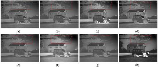
Figure 7.
Performance comparison of different fusion methods on the image pair “Marne”. (a–h) are the results of CVT, CWT, WLS, LP, ADF, GTF, MSVD and our algorithm, respectively.
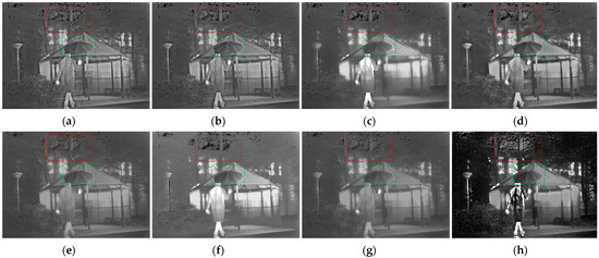
Figure 8.
Performance comparison of different fusion methods on the image pair “Umbrella”. (a–h) are the results of CVT, CWT, WLS, LP, ADF, GTF, MSVD and our algorithm, respectively.
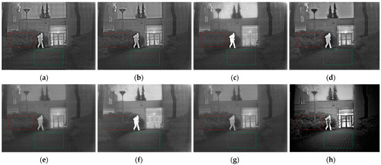
Figure 9.
Performance comparison of different fusion methods on the image pair “Kaptein”. (a–h) are the results of CVT, CWT, WLS, LP, ADF, GTF, MSVD and our algorithm, respectively.
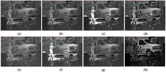
Figure 10.
Performance comparison of different fusion methods on the image pair “Car”. (a–h) are the results of CVT, CWT, WLS, LP, ADF, GTF, MSVD and our algorithm, respectively.
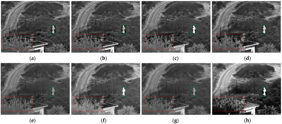
Figure 11.
Performance comparison of different fusion methods on the image pair “Camp”. (a–h) are the results of CVT, CWT, WLS, LP, ADF, GTF, MSVD and our algorithm, respectively.
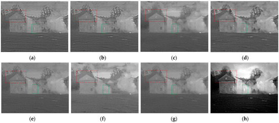
Figure 12.
Performance comparison of different fusion methods on the image pair “Octec”. (a–h) are the results of CVT, CWT, WLS, LP, ADF, GTF, MSVD and our algorithm, respectively.
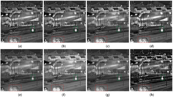
Figure 13.
Performance comparison of different fusion methods on the image pair “Road”. (a–h) are the results of CVT, CWT, WLS, LP, ADF, GTF, MSVD and our algorithm, respectively.
The fusion results of the first group on the “Marne” image pairs are shown in Figure 7. It is obvious that the most of fused images can contain rich textures of original visual image and the hot targets of infrared image. Furthermore, the cloud in the sky should be retained clearly in the final fused image as much as possible so that the fused image with higher contrast looks more natural. The results of the CVT, CWT and ADF algorithms own the lower contrast, so the visual quality of the fused image is a little bad. The algorithm of WLS can also improve the brightness distribution of the visible image, but the outline of the cloud in the red box does not look natural enough. The MSVD algorithm cannot fuse more edge and detail information into each layer of the image. In addition, the result of GTF algorithm is fused by more information from the infrared image, and the pattern on the car is the clearest. Although the CVT, WLS, LP, GTF and the proposed algorithm can preserve the target light regions, the proposed algorithm can transfer more textures of the cloud and the edges of the tree in visible images into the fused image.
Figure 8 exhibits the fusion results of the “Umbrella” image pair based on various fusion algorithms. Although all of these fusion methods in this paper can realize the aim of image fusion, the fusion effect of different fusion methods is still very different. The results of the CVT and CWT methods pay more attention to preserving the infrared areas of interest, but some components in the visible image are missing. The background of the WLS and GTF methods are over bright, which leads to the poor visual effect. The result based on the LP method owns better visual effect than Figure 8a, and the contrast of the background is not too bad, but it still needs to be improved. The diverse feature information cannot be extracted absolutely from the input images by the ADF and MSVD methods, so the results lose the significant information and tiny details, and the contrast is also low. Moreover, the result based on the method of this paper is suitable for the human visual perception system via enhancing the contrast of the interesting regions of the input images. In conclusion, the fused image of the “Umbrella” based on the proposed method contains more complementary information from the input images.
Next, the image pairs of “Kaptein” and “Car” are chosen as the test sets in order to affirm the effect of the proposed method further. The fusion results of the existing algorithms and ours are displayed in Figure 9 and Figure 10, respectively. It is very obvious that there are more noise and image artifacts in the fused images acquired by the methods of WLS and MSVD. In addition, the methods of the ADF and GTF cannot preserve more detail components of the visible image. Moreover, the background information is receiving more and more attention, and LP, CVT and CWT are proposed to keep more visual information. The final images fused by CVT, CWT and LP methods have more significant features and setting information. However, those images with so much complementary information look more similar to the infrared images, especially the background. Compared with the previous methods, the proposed algorithm can cut down the saliency features of the infrared image and the fused image is easier to be accepted. Furthermore, in Figure 9, the texture information in the ‘bushes’ (red box) and the ‘ground’ (green box) can be preserved as much as possible via our method, and the fused image is clearer and the detail information is more abundant.
In Figure 10, the fusion algorithms of CVT, CWT, LP and ours can reserve more salient features of the visible images. However, these results about the rest of the methods are fused by a lot of background information of the infrared image. By this way, it is very difficult to extract the salient components from the input image so that the background information and the context around the saliency regions are obscure and even not visible. Compared with the other fusion algorithms in this paper, our fusion method can fuse more detail components and keep the higher contrast of infrared components. The ‘tree’ in the red box of the fused image based on our method is clearer, and the detail information is richer than the others. Therefore, our method can maintain an optimal balance between the visual context information and the infrared saliency features.
In fact, our proposed method focuses on maintaining as much visible texture details as possible and highlighting the thermal target. Therefore, we hope that the experimental results based on our method can be more in line with human vision, and the large infrared targets will not be lost, such as the umbrella in the Figure 8, the human in the Figure 9 and Figure 10. However, the texture of the forest in Figure 8, the floor in Figure 9 and the trees in Figure 10 is clearer than other methods due to the omega correction in the Section 3.2, which can be used in greyscale images for changing their dynamic range and the local contrast. Of course, it is possible that these sets of experimental parameters are too biased towards the enhanced contrast of visible information, so they are a little darker. In addition, the adaptive adjustment of these parameters will also be our next task.
Moreover, it is necessary to prove the effect of retaining complementary information in this method. The fusion results based on different algorithms on the image “Camp” are displayed in Figure 11. The hot targets in the green box are clear enough on different methods. However, the contour of the figure in green box obtained by the methods of WLS and ours is more distinct and its brightness is improved greatly. In addition, the image details of the bushes in the red boxes reveal that the proposed algorithm possesses the following advantages. Firstly, the image contrast can be improved by the proposed method via enhancing the brightness of the bushes. Secondly, our algorithm can transmit more texture information of the bushes to the fused result so that the fused image looks more similar to the visible image and reserves much more infrared information.
In addition, the low contrast image pair “Octec” is selected to verify the fusion effect of our method. In Figure 12, there is some cloud of smoke in the center of the visual image, behind which the interesting target in the infrared image conceals. In addition, the fusion methods are ought to merge the hot target and the houses sheltered from the smoke into the result. CWT, WLS, LP and our algorithm all meet the above performance requirements. Moreover, the methods of the ADF and GTF can enhance the brightness of the fusion images, but the hot target in the green box is lost. Although the CWT algorithm improves the visual brightness of the fused result, the contrast of the fused image is very poor. In addition, the result of MSVD algorithm is without enough details of the trees and houses. As for CWT and GTF algorithms, the detail information of visible image cannot be reserved into the fused image so that the image looks a little blurry. Finally, the result obtained by the proposed method owns clearer detail information of the roof in the red box, and its contrast is more suitable for human vision.
Finally, the image pair “Road” taken at low illumination is chosen to experiment. In addition, the fusion results based on different algorithms are shown in the Figure 13.
As for the algorithms of CWT, WLS and ADF, the interesting parts such as the vehicles, the person and the lights are not able to be well highlighted. At the same time, the results of GTF and MSVD fusion algorithms do not conform to human eye vision observation due to its blurred details. Furthermore, the image contrast of the CVT and LP methods is better than the results obtained by the rest of the compared fusion algorithms. However, the proposed method can enhance the tiny features properly, for example, the person in the green box is clearer than the others, especially the outline between two legs; and the details of the car in the red box can also be preserved well. Therefore, the method proposed in this paper can meet the needs of night the observation.
Although the WLS and GTF can preserve more thermal characteristics than ours in Figure 8, Figure 9 and Figure 10, the visual detail components are not so much as ours. For example, the texture features of the bush in Figure 8 and Figure 9 are richer. Of course, this also shows that our algorithm can integrate more visual significant features of the visible image into the fused image. Moreover, there are some small infrared detail information lost in ours, such as the brightness information on the human in Figure 10. However, this will not affect our recognition of infrared targets. Of course, our next focus will also be to find a better way to balance while retaining more infrared and visible information.
In conclusion, obviously, our method can not only improve the contrast of the fusion images, but also fuse more infrared brightness features in each experiment. Although the compared methods can also highlight the interesting parts of input images, they cannot fuse more details of the input images such as this method. In a word, the proposed algorithm in this paper can achieve a better balance between highlighting infrared targets and reserving detail information, and the results are easier to be accepted by human eyes.
4.3. Objective Evaluation
Five fusion quality evaluation metrics are selected to evaluate our fusion algorithm objectively, such as average gradient (AVG) [46], mutual information (MI) [47], edge strength (Qab/f) [30], spatial frequency (SF) [48] and standard deviation (SD) [49]. The fusion performance improves with the eight methods of all these five metrics, and the results are shown in Table 1.

Table 1.
The objective evaluation results for experiments.
The evaluation results are shown in Table 1, in which the values marked in bold are the best of all. From the 7 experiments, we can see that the AVG value of the proposed algorithm is higher than the other algorithms besides the fourth experiment, which indicates that our algorithm can keep the gradient texture information contained in the original images into the fusion image, and our fused images have the most abundant detail information. The amount of the edge information can be counted by the metric of Qab/f, which represents the ability that the edges are shifted to the fused images from the input images. We can clearly see that in addition to the second to forth group of experiments, the Qab/f values of our algorithm keeps leading. This shows again that our method owns the prominent effect both on the reconstruction and restoration of the gradient information. As for the evaluation of SF and SD values, the SF value indicates the global activities of the image in the domain of the space, and the value of SD is used to reflect the gray-value distribution of each pixel, which is another manifestation of sharpness and is computed indirectly by the average values of the image. Both SF and SD values of other methods are lower than the proposed algorithm, so the result of our proposed method has the higher overall activity in the spatial domain and the contrast of the image is promoted well. MI characterizes the degree of correlation between the fused image and the original image. Except the fourth group of experiment, the values of other methods perform better than ours, which indicates that the proposed algorithm in this aspect still needs to be improved.
5. Conclusions
This paper proposed a novel fusion model for infrared and visual images based on co-occurrence analysis shearlet transform. Firstly, the CAST is used as the multi-scale transform tool to decompose the source images. Next, for the base-layer images that represent the energy distribution, we adopt the LatLRR to generate the saliency maps, and a weighted model guided by the salient map is put forward as the fusion rule. For the detail-layer images that reflect the texture detail information, an optimization model based on zero-crossing counting regularization is adopted as the fusion rule. In order to confirm the performance of our method, relevant experiments are implemented in this paper. The results show that the fused images obtained by ours with a higher contrast and rich texture detail information outperform the others in terms of visual evaluation.
Author Contributions
Conceptualization, B.Q.; methodology, B.Q.; validation, B.Q., L.J. and W.W.; investigation, B.Q. and Y.Z.; resources, L.J., G.L. and Q.L.; writing—original draft preparation, B.Q.; writing—review and editing, L.J. and G.B. All authors have read and agreed to the published version of the manuscript.
Funding
This work was supported in part by the National Natural Science Foundation of China under Grant 61801455.
Data Availability Statement
Not applicable.
Conflicts of Interest
The authors declare no conflict of interest.
References
- Palsson, F.; Sveinsson, J.; Ulfarsson, M. Sentinel-2 Image Fusion Using a Deep Residual Network. Remote Sens. 2018, 18, 1290. [Google Scholar] [CrossRef] [Green Version]
- Liu, Y.; Dong, L.; Chen, Y.; Xu, W. An Efficient Method for Infrared and Visual Images Fusion Based on Visual Attention Technique. Remote Sens. 2020, 12, 781. [Google Scholar] [CrossRef] [Green Version]
- Chen, J.; Wu, K.; Cheng, Z.; Luo, L. A Saliency-based Multiscale Approach for Infrared and Visible Image Fusion. Signal Process. 2021, 182, 4–19. [Google Scholar] [CrossRef]
- Harbinder, S.; Carlos, S.; Gabriel, C. Construction of Fused Image with Improved Depth-of-field Based on Guided Co-occurrence Filtering. Digit. Signal Process. 2020, 104, 516–529. [Google Scholar]
- Li, H.; Wu, X.; Josef, K. MDLatLRR: A Novel Decomposition Method for Infrared and Visible Image Fusion. IEEE Trans. Image Process. 2020, 29, 4733–4746. [Google Scholar] [CrossRef] [Green Version]
- Shen, D.; Masoumeh, Z.; Yang, J. Infrared and Visible Image Fusion via Global Variable Consensus. Image Vis. Comput. 2020, 104, 153–178. [Google Scholar] [CrossRef]
- Bavirisetti, D.; Xiao, G.; Liu, G. Multi-sensor Image Fusion Based on Fourth Order Partial Differential Equations. In Proceedings of the 2017 20th International Conference on Information Fusion (Fusion), Xi’an, China, 10–13 July 2017; pp. 1–9. [Google Scholar]
- Zhao, W.; Lu, H.; Dong, W. Multisensor Image Fusion and Enhancement in Spectral Total Variation Domain. IEEE Trans. Image Process. 2018, 20, 866–879. [Google Scholar] [CrossRef]
- Tan, W.; William, T.; Xiang, P.; Zhou, H. Multi-modal Brain Image Fusion Based on Multi-level Edge-preserving Filtering. Biomed. Signal Process. Control 2021, 64, 1882–1886. [Google Scholar] [CrossRef]
- Peter, B.; Edward, A. The Laplacian Pyramid as a Compact Image Code. IEEE Trans. Commun. 1983, 31, 532–540. [Google Scholar]
- Liu, J.; Ding, J.; Ge, X.; Wang, J. Evaluation of Total Nitrogen in Water via Airborne Hyperspectral Data: Potential of Fractional Order Discretization Algorithm and Discrete Wavelet Transform Analysis. Remote Sens. 2021, 13, 4643. [Google Scholar] [CrossRef]
- Wang, Z.; Xu, J.; Jiang, X.; Yan, X. Infrared and Visible Image Fusion via Hybrid Decomposition of NSCT and Morphological Sequential Toggle Operator. Optik 2020, 201, 163497. [Google Scholar] [CrossRef]
- Cheng, B.; Jin, L.; Li, G. A Novel Fusion Framework of Visible Light and Infrared Images Based on Singular Value Decomposition and Adaptive DUALPCNN in NSST Domain. Infrared Phys. Technol. 2018, 91, 153–163. [Google Scholar] [CrossRef]
- Zhuang, P.; Zhu, X.; Ding, X. MRI Reconstruction with an Edge-preserving Filtering Prior. Signal Process. 2019, 155, 346–357. [Google Scholar] [CrossRef]
- Yin, H.; Gong, Y.; Qiu, G. Side Window Guided Filtering. Signal Process. 2019, 165, 315–330. [Google Scholar] [CrossRef]
- Gong, Y.; Sbalzarini, I. Curvature Filters Efficiently Reduce Certain Variational Energies. IEEE Trans. Image Process. 2017, 26, 1786–1798. [Google Scholar] [CrossRef] [Green Version]
- Tomasi, C.; Manduchi, R. Bilateral Filtering for Gray and Color Images. In Proceedings of the Sixth International Conference on Computer Vision (IEEE Cat. No. 98CH36271), Bombay, India, 7 January 1998; IEEE: Piscataway, NJ, USA, 2002; pp. 839–846. [Google Scholar]
- He, K.; Sun, J.; Tang, X. Guided Image Filtering. IEEE Trans. Pattern Anal. Mach. Intell. 2012, 35, 1397–1409. [Google Scholar] [CrossRef]
- Yuan, W.; Yuan, X.; Xu, S.; Gong, J.; Shibasaki, R. Dense Image-Matching via Optical Flow Field Estimation and Fast-Guided Filter Refinement. Remote Sens. 2019, 11, 2410. [Google Scholar] [CrossRef] [Green Version]
- Liu, S.; Zhao, J.; Shi, M. Medical Image Fusion Based on Rolling Guidance Filter and Spiking Cortical Mode. Comput. Math. Methods Med. 2015, 2015, 156043. [Google Scholar]
- Jevnisek, R.; Shai, A. Co-occurrence Filter. In Proceedings of the IEEE Conference on Computer Vision and Pattern Recognition, Honolulu, HI, USA, 21–26 July 2017. [Google Scholar]
- Liu, G.; Yan, S. Latent Low-rank Representation for Subspace Segmentation and Feature Extraction. In Proceedings of the IEEE International Conference on Computer Vision (ICCV), Barcelona, Spain, 6–13 November 2011; pp. 1615–1622. [Google Scholar]
- Nie, T.; Huang, L.; Liu, H.; Li, X.; Zhao, Y.; Yuan, H.; Song, X.; He, B. Multi-Exposure Fusion of Gray Images Under Low Illumination Based on Low-Rank Decomposition. Remote Sens. 2021, 13, 204. [Google Scholar] [CrossRef]
- Cheng, B.; Jin, L.; Li, G. General Fusion Method for Infrared and Visual Images via Latent Low-rank Representation and Local Non-subsampled Shearlet Transform. Infrared Phys. Technol. 2018, 92, 68–77. [Google Scholar] [CrossRef]
- Jiang, X.; Yao, H.; Liu, S. How Many Zero Crossings? A Method for Structure-texture Image Decomposition. Comput. Graph. 2017, 68, 129–141. [Google Scholar] [CrossRef]
- Cheng, B.; Jin, L.; Li, G. Infrared and Low-light-level Image Fusion Based on l2-energy Minimization and Mixed-L1-gradient Regularization. Infrared Phys. Technol. 2019, 96, 163–173. [Google Scholar] [CrossRef]
- Zhang, P. Infrared and Visible Image Fusion Using Co-occurrence Filter. Infrared Phys. Technol. 2018, 93, 223–231. [Google Scholar] [CrossRef]
- Hu, Y.; He, J.; Xu, L. Infrared and Visible Image Fusion Based on Multiscale Decomposition with Gaussian and Co-Occurrence Filters. In Proceedings of the 4th International Conference on Pattern Recognition and Artificial Intelligence (PRAI), Yibin, China, 20–22 August 2021. [Google Scholar]
- Wang, B.; Zeng, J.; Lin, S.; Bai, G. Multi-band Images Synchronous Fusion Based on NSST and Fuzzy Logical Inference. Infrared Phys. Technol. 2019, 98, 94–107. [Google Scholar] [CrossRef]
- Ma, J.; Zhou, Z.; Wang, B.; Zong, H. Infrared and Visible Image Fusion Based on Visual Saliency Map and Weighted Least Square Optimization. Infrared Phys. Technol. 2017, 82, 8–17. [Google Scholar] [CrossRef]
- Marr, D.; Ullman, S.; Poggio, T. Bandpass Channels, Zero-crossings, and Early Visual Information Processing. J. Opt. Soc. Am. 1979, 69, 914–916. [Google Scholar] [CrossRef]
- Combettes, P.; Pesquet, J. Proximal splitting methods in signal processing. In Fixed-Point Algorithms for Inverse Problems in Science and Engineering; Bauschke, H., Burachik, R., Combettes, P., Elser, V., Luke, D., Wolkowicz, H., Eds.; Springer: New York, NY, USA, 2011; pp. 185–212. [Google Scholar]
- Zakhor, A.; Oppenheim, A. Reconstruction of Two-dimensional Signals from Level Crossings. Proc. IEEE 1990, 78, 31–55. [Google Scholar] [CrossRef]
- Badri, H.; Yahia, H.; Aboutajdine, D. Fast Edge-aware Processing via First Order Proximal Approximation. IEEE Trans. Vis. Comput. Graph. 2015, 21, 743–755. [Google Scholar] [CrossRef]
- Boyd, S.; Parikh, N.; Chu, E.; Peleato, B.; Eckstein, J. Distributed Optimization and Statistical Learning via the Alternating Direction Method of Multipliers. Found. Trends Mach. Learn. 2011, 3, 1–122. [Google Scholar]
- Storath, M.; Weinmann, A.; Demaret, L. Jump-sparse and Sparse Recovery Using Potts Functionals. IEEE Trans. Signal Process. 2014, 62, 3654–3666. [Google Scholar] [CrossRef] [Green Version]
- Storath, M.; Weinmann, A. Fast Partitioning of Vector-valued Images. SIAM J. Imaging Sci. 2014, 7, 1826–1852. [Google Scholar] [CrossRef] [Green Version]
- Ono, S. l0 Gradient Projection. IEEE Trans. Image Process. 2017, 26, 1554–1564. [Google Scholar] [CrossRef] [PubMed]
- Ren, L.; Pan, Z.; Cao, J.; Liao, J.; Wang, Y. Infrared and Visible Image Fusion Based on Weighted Variance Guided Filter and Image Contrast Enhancement. Infrared Phys. Technol. 2021, 114, 71–77. [Google Scholar] [CrossRef]
- Toet, A. TNO Image Fusion Dataset. 2014. Available online: https://figshare.com/articles/TN_Image_Fusion_Dataset/1008029 (accessed on 30 November 2021).
- Cai, W.; Li, M.; Li, X. Infrared and Visible Image Fusion Scheme Based on Contourlet Transform. In Proceedings of the Fifth International Conference on Image and Graphics (ICIG), Xi’an, China, 20–23 September 2009; IEEE: Piscataway, NJ, USA, 2009; pp. 20–23. [Google Scholar]
- John, J.; Robert, J.; Stavri, G.; David, R.; Nishan, C. Pixel-and Region-based Image Fusion with Complex Wavelets. Inf. Fusion 2007, 8, 119–130. [Google Scholar]
- Liu, Y.; Liu, S.; Wang, Z. A General Framework for Image Fusion Based on Multi-scale Transform and Sparse Representation. Inf. Fusion 2015, 24, 147–164. [Google Scholar] [CrossRef]
- Ma, J.; Chen, C.; Li, C.; Huang, J. Infrared and Visible Image Fusion via Gradient Transfer and Total Variation Minimization. Inf. Fusion 2016, 31, 100–109. [Google Scholar] [CrossRef]
- Naidu, V. Image Fusion Technique Using Multi-resolution Singular Value Decomposition. Def. Sci. J. 2011, 61, 479–484. [Google Scholar] [CrossRef] [Green Version]
- Jin, H.; Xi, Q.; Wang, Y. Fusion of visible and infrared images using multi objective evolutionary algorithm based on decomposition. Infrared Phys. Technol. 2015, 71, 151–158. [Google Scholar] [CrossRef]
- Li, H.; Wu, X.; Kittler, J. RFN-Nest: An End-to-end Residual Fusion Network for Infrared and Visible Images. Inf. Fusion 2021, 73, 72–86. [Google Scholar] [CrossRef]
- Eskicioglu, A.M.; Fisher, P. Image quality measures and their performance. IEEE Trans. Commun. 1995, 43, 2959–2965. [Google Scholar] [CrossRef] [Green Version]
- Qu, G.; Zhang, D.; Yan, P. Information measure for performance of image fusion. Electron. Lett. 2002, 38, 313–315. [Google Scholar] [CrossRef] [Green Version]
Publisher’s Note: MDPI stays neutral with regard to jurisdictional claims in published maps and institutional affiliations. |
© 2022 by the authors. Licensee MDPI, Basel, Switzerland. This article is an open access article distributed under the terms and conditions of the Creative Commons Attribution (CC BY) license (https://creativecommons.org/licenses/by/4.0/).