Article

Spatiotemporal Variation in Vegetation Growth Status and Its Response to Climate in the Three-River Headwaters Region, China

1
Institute of Ecological Conservation and Restoration, Chinese Academy of Forestry, Beijing 100091, China
2
Institute of Desertification Studies, Chinese Academy of Forestry, Beijing 100091, China
3
National Climate Center, China Meteorological Administration, Beijing 100081, China
*
Author to whom correspondence should be addressed.
Remote Sens. 2022, 14(19), 5041; https://doi.org/10.3390/rs14195041
Submission received: 26 August 2022 / Revised: 29 September 2022 / Accepted: 5 October 2022 / Published: 9 October 2022

Abstract

:
The Three-River Headwaters Region (TRHR), located in the hinterland of the Qinghai–Tibet Plateau (QTP), is an important water-conservation and ecological-function reserve in China. Studies of the growth of vegetation in the TRHR and its response to climate under the background of global warming are of great relevance for ecological protection of the QTP. In this study, based on MOD13Q1 Enhanced Vegetation Index (EVI) data and ERA5-Land climate data, the ensemble empirical mode decomposition method, random forest algorithm, and Hurst exponent were used to detect the spatiotemporal dynamics and response to climate change in TRHR vegetation during 2000–2021. The results indicated the following. (1) Comparatively, the condition of vegetation growth was better in 2021, 2010, and 2018 and poorer in 2015, 2003, and 2008. The EVI gradually decreased from the southeast to the northwest, and the area of improved vegetation growth was larger than the area of degraded vegetation growth. (2) The area of zones with either monotonous greening or monotonous browning of vegetation was 30.30% and 6.30%, respectively, and the trend of reversed vegetation change occurred in 63.40% of the areas. The area of future degradation of vegetation in the TRHR was larger than the area of future improvement, and the risk of vegetation degradation was higher. (3) Precipitation and soil temperature are the main and secondary driving factors of vegetation change in the TRHR, respectively. Warming and humidification of the QTP climate play major roles in the improvement of vegetation growth in the TRHR.

1. Introduction

As an important part of Earth’s surface and terrestrial ecosystems, vegetation links the exchange of materials and energy between soil, water bodies, and the atmosphere, and is an important indicator of the physical geographic environment [1,2,3]. Climate change has a direct impact on the status and trends of vegetation growth [4], and vegetation can also feed back into climate change by regulating the water–carbon cycle and energy flow [5,6]. According to the latest assessment by the Intergovernmental Panel on Climate Change, the global concentration of atmospheric CO2 has increased from 285 ppmv in the second half of the 19th century (1850–1900) to 414 ppmv in 2020, and the average global temperature has increased concurrently by 1.09 °C [7]. In recent years, global warming has led to the frequent occurrence of extreme weather events such as floods, high temperatures, and droughts, which have had a huge impact on terrestrial ecosystems [8,9,10]. Therefore, studying the growth and trends of changes in vegetation, comprehensively quantifying the impact of climatic constraints on the growth of terrestrial vegetation, and improving our understanding of the dynamic response mechanisms of vegetation are of great relevance for the accurate prediction of future vegetation trends, ecosystem evolution, and global change, and for the effective implementation of macro-environmental management.
Monitoring vegetation growth using remote sensing technology has the advantages of being macroscopic, dynamic, economical, and efficient. Vegetation indexes provide potential for monitoring vegetation cover on a large scale and for a long period, and have produced reasonable results in reflecting changes in vegetation growth [11,12]. With the increase in the volume of archived remote sensing data and the impact of multisensor technology, recent research has undertaken analysis of long time series of vegetation using vegetation indexes at different spatiotemporal scales. For example, vegetation dynamics on the Qinghai–Tibet Plateau (QTP) were investigated by both Peng [13] and Chen [14] using AVHRR data and MODIS data, respectively, and their results revealed that QTP vegetation has undergone a continuous greening process since 1983. Bai [15] used AVHRR data to analyze the growth trend of vegetation in the Three-River Headwaters Region (TRHR) in China and its response to climate during 1982–2015. Zhai [16] used MODIS data inversion to assess the aboveground net primary productivity of the main vegetation types at different stages of growth in the TRHR. The use of long time series of remote sensing imagery provides a robust scientific approach for the accurate evaluation of long-term changes in vegetation growth. Moreover, among the dozens of proposed vegetation indexes, the Enhanced Vegetation Index (EVI), which can correct for both soil and atmospheric noise, has a great ability to distinguish vegetation in areas of sparse vegetation and has been widely used in research to evaluate vegetation change [17]. Vegetation is sparse in large areas of the TRHR, and therefore, the EVI is considered suitable for reflecting local vegetation growth.
The vegetation growth trend is an indicator of local hydrothermal activities and can reflect the impact of climate change on terrestrial ecosystems [18]. Most previous related studies used linear regression analysis, which adopts a constant rate to determine the trend of a single raster over a long period, thereby reflecting the spatiotemporal patterns of regional vegetation change. However, vegetation trends are nonlinear and varied, and linear regression methods might ignore internal abrupt changes and trend shifts, thereby obscuring the true trends of vegetation change. Ensemble empirical mode decomposition (EEMD) can divide a nonstationary time series into a finite set of components with decreasing frequency and a long-term trend [19]. The long-term trend extracted by EEMD is monotonic or contains only one extreme value, and the variability varies with time. Moreover, such long-term trends do not need to follow a priori assumptions and are insensitive to expansion of the time series [20]. This property allows long-term trends extracted using EEMD to reveal more fundamental information about nonlinear and nonstationary vegetation time series [18]. The effectiveness of EEMD in monitoring the dynamics and trend shifts of long time series of vegetation has been proven in previous research [21,22].
The TRHR, which is located in the central part of the QTP, is the source area of the Yangtze, Yellow, and Lancang rivers and is known as the “Asian Water Tower.” Since the 1950s, the QTP has experienced a uniform trend of warming that is almost twice the global rate of warming [23,24], and this trend is expected to continue until the end of the 21st century [25]. Concurrently, precipitation on the QTP has shown a slight increase and strong spatial heterogeneity [26], and the overall warming and humidification of the QTP have become increasingly pronounced. The TRHR is sensitive and responsive to global warming, and climate change might have a substantial impact on the growth of QTP vegetation [27,28]. Owing to the complexity and nonlinearity of the response relationship between vegetation and climate change, it is difficult to describe the interrelationships between vegetation and climatic factors in a single regression equation [29]. Since 2000, under the background of global warming and socioeconomic development, the impact of humans on the TRHR has reached a new level. To understand the mechanism of the observed changes in alpine meadow in the context of global warming, as well as to provide theoretical support for sustainable development of the ecology, economy, and society of the QTP, it is important to study vegetation growth in the TRHR and its response to climate. Therefore, this study used MODIS EVI data and ERA5-Land climate data to determine the spatiotemporal dynamics of vegetation in the TRHR over the past 20 years and to reveal its spatiotemporal response to climate.
The objectives of this study were as follows: (1) to analyze the spatiotemporal characteristics of vegetation growth in the study area over the past 20 years, (2) to analyze the trend change characteristics of vegetation growth and its future trend prediction, and (3) to identify the main climatic factors affecting vegetation change through quantitative spatiotemporal analysis.

2. Study Area and Data

2.1. Study Area

The TRHR is located in the south of Qinghai Province in China (31°38′–36°20′N, 89°31′–102°14′E), covering an area of approximately 363,000 km2 (Figure 1). The TRHR is the source region of the Yangtze River, Yellow River, and Lancang River, and is known as the Asian Water Tower. It is an area with a fragile ecological environment that is sensitive to the effects of climate change. The average elevation of the terrain of the TRHR is >4000 m. The average annual temperature is between −5.6 and 4.9 °C, and the mean temperature difference between day and night can exceed 20 °C. Annual precipitation is in the range of 390–764 mm, and precipitation is mainly concentrated during June–September. The eastern part of the TRHR is wetter and has more precipitation than the western part, which is arid and semiarid with less precipitation. The region has a continental plateau-type climate with distinct hot/cold and alternating wet/dry seasons. The distributions of soil and vegetation have the common characteristic of obvious vertical change. With increasing elevation, the soil type changes from alpine steppe soil to alpine meadow soil, and to alpine cold desert soil. The main vegetation type is grassland, which accounts for approximately 70% of the total area. The main grassland types are alpine grassland, alpine meadow, and sparse grassland.

2.2. Data and Processing

MOD13Q1-EVI (V006) data from 2001 to 2021, obtained from NASA’s Land Processes Distributed Active Archive Center, were used in this study. The MOD13Q1-EVI product is a 16-day synthetic vegetation index with a 250 m spatial resolution. The data can be used for monitoring global vegetation conditions and for characterizing surface biophysical properties and processes, indicating land cover change. The method of determining the common maximum-value composite of the annual maximum EVI images was used to investigate the spatiotemporal change in vegetation in the study area.
The climate data used in the study comprised the 2 m temperature (air temperature at 2 meters above the surface of the land, sea, or in-land waters, TMP), soil temperature level 2 (STMP), total precipitation (PRE), surface pressure (SP), and surface net solar radiation (SSR) data extracted from the ERA5-Land climate data with a 0.1° resolution (https://cds.climate.copernicus.eu/ (accessed on 20 April 2022)). The diurnal temperature difference in the TRHR is large, and the surface soil temperature is more susceptible to external environmental effects; therefore, the STMP at 7–20 cm was used to represent ground temperature. In this research, 250 m spatial resolution EVI data were used for analyzing the spatiotemporal characteristics of vegetation growth, while for the analysis of vegetation response to climate, the EVI data were resampled to a 0.1° resolution using the nearest interpolation method in order to be consistent with the climate data.
Land cover type data were obtained from the global 30 m land cover product with a fine classification system for 2020 (https://data.casearth.cn/ (accessed on 20 April 2022)), and water bodies and permanent snow and ice were removed for improved accuracy. The digital elevation model data were derived from the Shuttle Radar Topography Mission data, jointly measured by NASA and the National Imagery and Mapping Agency, with a 90 m spatial resolution.

3. Methodology

3.1. Linear Regression Analysis

Trend analysis based on the linear regression method can appropriately reflect the spatiotemporal patterns of vegetation change in the study region [22]. The trend of EVI changes in the TRHR during 2000–2021 was analyzed using linear regression, and the spatial characteristics of the vegetation changes in different periods were examined. The specific calculation formula is as follows:
S l o p e = n i = 1 n ( i E V I i ) ( i = 1 n i ) ( i = 1 n E V I i ) n i = 1 n i 2 ( i = 1 n i ) 2
where n is the total number of years in the time period, EVIi is the annual maximum EVI value in the i-th year, and Slope is the change rate of the regression equation. Slope > 0 means that the EVI value had an increasing trend during the 22-year period; conversely, Slope < 0 means that the EVI value had a decreasing trend.

3.2. Coefficient of Variation

Standard deviation (SD) and coefficient of variation (CV) are used widely as important indicators in quantitative evaluation of the dispersion of an array. SD is a measure of the degree of dispersion of a set of values from the mean. CV, as a statistical measure of the degree of variation of each observation in a data set, is the ratio of the SD to the mean, which can eliminate the influence of different units or means on the comparison of the degree of variation of two or more data sets to reflect the degree of dispersion of the unit mean. The equations for the calculation of SD and CV can be expressed as follows:
σ = 1 n i = 1 n ( x i x ¯ ) 2 ( i = 1 , 2 , 3 )
C V = σ μ ,
where σ is the SD, μ is the mean of the EVI array, x is the array (in this study, EVI), and i and n are the numbers of years in 2000–2021.

3.3. EEMD Method

The EEMD method is based on empirical mode decomposition, and can be used to decompose a nonstationary time series into a finite set of decreasing frequency components (intrinsic mode functions (IMFs)) and a residual long-term trend. The extracted long-term trend is monotonic or contains only a single extreme value, varies over time, and shows no abrupt variation in the rate of change. More importantly, this long-term trend does not need to follow a predetermined functional form and is insensitive to the expansion of the time series. In this study, we decomposed the nonlinear trend of vegetation change and its succession over time using the EEMD method. The specific steps adopted were as follows.
Step 1: Add Gaussian white noise w1(t) to the original data x(t). The amplitude of the white noise is 0.2 times the SD of the original data:
x 1 ( t ) = x ( t ) + w 1 ( t )
Step 2: Connect all the maximal and minimal points with three spline curves to form the upper and lower envelopes of the new time series data x1(t), respectively. Then, subtract the mean value m1(t) of the upper and lower envelopes from the new time series data x1(t):
f 1 ( t ) = x 1 ( t ) m 1 ( t )
Step 3: Determine whether m1(t) satisfies the stopping condition (close enough to zero at any point). If the stopping condition is satisfied, the decomposition is topped; otherwise, take f1(t) as the new time series data and repeat step 2. Eventually, the first IMF (imf1(t)) is obtained:
f 2 ( t ) = f 1 ( t ) m 2 ( t ) ,
i m f 1 ( t ) = f k ( t ) = f k 1 ( t ) m k ( t ) .
Step 4: Subtract imf1(t) from x1(t) to obtain the remaining quantity R1(t). Repeat steps 2 and 3 with R1(t) as the new time series data if R1(t) still contains an oscillatory component:
R 1 ( t ) = x 1 ( t ) i m f 1 ( t ) ,
R n ( t ) = R n 1 ( t ) i m f n ( t ) ,
Thus, x1(t) is decomposed into a series of IMFs with decreasing frequency and a trend term that is monotonic or has, at most, a single extreme point:
x 1 ( t ) = j = 1 n i m f j ( t ) + R n ( t ) .
Step 5: Repeat steps 1–4 i times (here, i was set to 1000), adding a different Gaussian white noise sequence to the original data each time, and finally, using the average value obtained from these calculations as the final result. In this study, the analysis was implemented in R software using the ‘Rlibeemd’ package [30].
The EVI time series data were classified into four trends according to the properties of monotonicity and extreme value points obtained from the EEMD method:
Greening-to-greening (G to G)/browning-to-browning (B to B): the trends were monotonically increasing/decreasing;
Greening-to-browning (G to B)/browning-to-greening (B to G): the trends contained a single local maximum/minimum.

3.4. Hurst Exponent Method

To predict future trends in vegetation and to assess the sustainability of the time series, the Hurst exponent method based on the Rescaled Range Analysis (R/S) was used. The Hurst exponent, proposed by the British hydrologist Hurst [31], is used widely in the fields of hydrology, economics, climatology, and ecology [14,32,33]. The main equations can be expressed as in the following.
Step 1: Divide the long time series {EVI (t)} (τ = 1, 2, …, n) into τ subseries X (t), and for each series, t = 1, …, τ.
Step 2: Define the long-term memory of the time series of the mean EVI:
E V I ( τ ) ¯ = 1 τ t = 1 τ E V I ( τ ) τ = 1 , 2 , , n .
Step 3: Calculate the cumulative deviation:
X ( t , τ ) = u = 1 t ( E V I ( u ) E V I ( τ ) ¯ ) 1 t τ .
Step 4: Create the range sequence:
R ( τ ) = max 1 t τ X ( x , τ ) min 1 t τ X ( t , τ ) τ = 1 , 2 , , n .
Step 5: Create the SD sequence:
S ( τ ) = [ i τ t = 1 τ ( E V I ( t ) E V I ( τ ) ) 2 ] 1 2 .
Step 6: Calculate the Hurst exponent:
R ( τ ) / S ( τ ) = τ H .
The Hurst exponent varies in the range of 0–1 and can be categorized into three cases. If H is close to 0.5, it indicates that the time series is an independent random series and that the future trend is independent of the trend during the study period. If 0.5 < H, it indicates that the time series is persistent and that the future trend is consistent with that of the past, and the closer the value of H is to 1, the stronger the persistence. If H < 0.5, it indicates that the time series has inverse persistence, where the future trend is the opposite to that of the past, and the closer the value of H is to 0, the stronger the inverse persistence.

3.5. Correlation Analysis

The correlation coefficient measures the linear relationship between two variables. In this study, the correlation coefficients between the EVI and the climatic factors were calculated using the Pearson correlation method, which can be expressed mathematically as follows:
r = i = 1 n ( x i x ¯ ) ( y i y ¯ ) i = 1 n ( x i x ¯ ) 2 i = 1 n ( y i y ¯ ) 2
where r is the correlation coefficient, and x ¯ and y ¯ are the means of the respective variables. The correlation coefficient has a range of −1 to 1, and the closer its value is to −1 or 1, the stronger the correlation between the variables.

3.6. Random Forest Model

The RF is a machine learning method consisting of an ensemble of randomized classification and regression trees, where a random subsample is constructed for each tree, and the final result is obtained by voting on the modeling results of all trees [34]. The RF algorithm reduces the computational effort while improving prediction accuracy. Moreover, the algorithm is insensitive to multivariate covariance, is robust to missing and unbalanced data, and can be well adapted to data sets with up to several thousand explanatory variables [35,36]. The RF algorithm uses the increase in node purity (IncNodePurity) as an estimate of the importance of the predictor variables. IncNodePurity is measured by the sum of the squared residuals and represents the effect of each variable on the heterogeneity of observations at each node of the classification tree, where a larger value indicates greater importance of the variable.
The EVI and the climate data from 2000 to 2021 were discretized into 22 periods of raster data with EVI as the dependent variable and the climatic factors as the independent variables, and the EVI was fitted based on RF regression to qualitatively analyze the spatial influence of climatic factors on the EVI. In this process, 70% of the data were randomly selected for modeling, and the remaining 30% of the data were used for model accuracy validation. The analysis was implemented in R software using the ‘randomForest’ package [37].

4. Results and Analysis

4.1. Spatiotemporal Characteristics of Vegetation Growth

4.1.1. Temporal Characteristics of Vegetation Growth

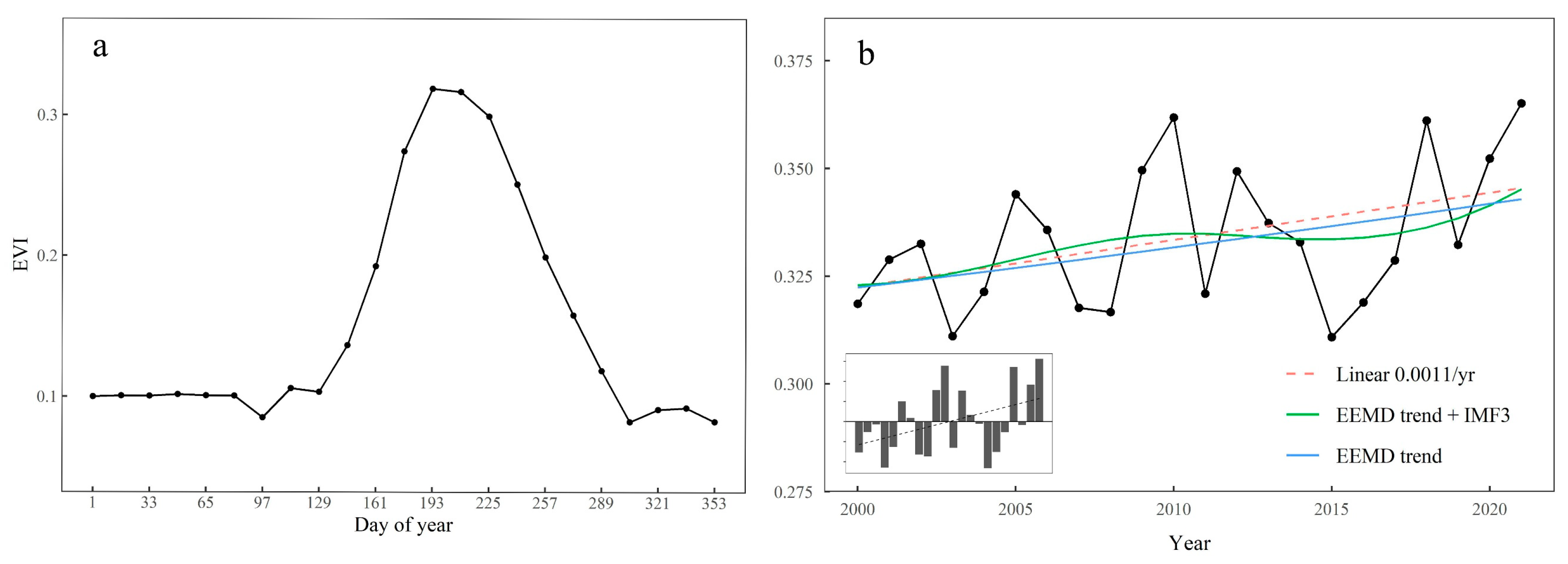
The TRHR is located in the hinterland of the QTP and has a typical plateau continental climate. Generally, the coldest time in each region of the TRHR is January, and the hottest time in most regions is July, with an annual average temperature of between −8.6 and 4.9 °C. Precipitation is concentrated in summer, with up to 80% of the total rainfall occurring during May–September [28,29]. The effect of rain and heat in the same period caused the vegetation index change curve of the TRHR to show a single-peaked wave during the year (Figure 2a). In terms of vegetation growth, the EVI increased constantly in early May, when the temperature rose and the permafrost layer gradually thawed, and vegetation in the TRHR began to sprout and grow. In summer, the vegetation grew under the suitable hydrological and thermal conditions, and the amount of precipitation and snow meltwater increased. Thus, the EVI gradually increased and reached its annual peak in mid-July. In autumn and winter, as the temperature dropped markedly, most of the leaves of the vegetation began to wither, and the EVI declined gradually, reaching its lowest point in late October.
In terms of interannual change, the multiyear average EVI of the TRHR was 0.3340 between 2000 and 2021. The years in which the departure from the average EVI (hereafter, expressed as ΔEVI) was positive were mainly 2009, 2010, 2018, 2020, and 2021, with the highest ΔEVI of 0.0312, 0.0279, and 0.0271 in 2021, 2010, and 2018 at 0.0312 and 0.0279, respectively. The years with negative ΔEVI were mainly 2003, 2007, 2008, 2015, and 2016, with the lowest EVI of −0.0231, −0.0229, and −0.0173 in 2015, 2003, and 2008, respectively. During 2000–2021, the average EVI of the TRHR increased slowly at a rate of 0.0011/a (p < 0.001) (Figure 2b). Using image scales to calculate the difference between the annual EVI and the average EVI revealed that during 2000–2021, the EVI of the TRHR was dominated by slight fluctuations, with the area of −0.1 < ΔEVI < 0.1 accounting for more than 91.88% of the total area. The area of −0.1 < ΔEVI < 0 was the largest in 2015, followed by 2003, accounting for 77.82% and 77.57% of the total area, respectively. The area of 0 < ΔEVI < 0.1 was the largest in 2021, followed by 2010, accounting for 69.78% and 63.23% of the total area, respectively.

4.1.2. Spatial Characteristics of Vegetation Growth

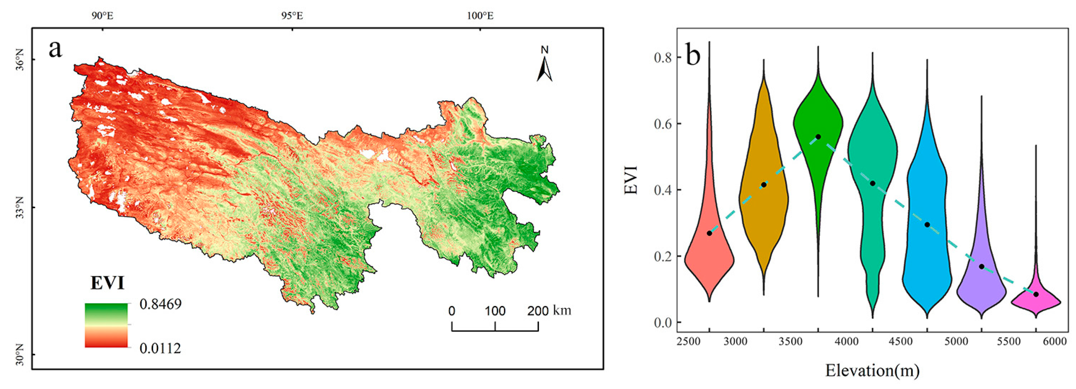
The variation in the EVI in the TRHR during 2000–2021 ranged from 0.0112 to 0.8469, and the vegetation showed a gradual decline from the southeast to the northwest (Figure 3a). Areas of low vegetation cover (EVI < 0.3) accounted for 46.32% of the study area, and were mainly distributed in higher elevation areas such as the western and northern parts of the TRHR. Areas of medium vegetation cover (0.3 ≤ EVI < 0.6) were mainly distributed in central parts of the TRHR. Areas of high vegetation cover (EVI ≥ 0.6) were mainly distributed in the Yellow River source area in the east and the Lancang River source area in the south, where elevation is lower and the vegetation types are mainly forest and scrub.
The topography of the TRHR area is complex, and differences in elevation greatly affect the types and growth conditions of regional vegetation. The distribution of the EVI within the TRHR interval was calculated using a 500 m elevation interval (Figure 3b). In the TRHR, the elevation of 2500–3000 m is relatively low and the area of distribution of human settlements is comparatively large. The process of urbanization and the intensity of human activities have a great impact on vegetation growth in the TRHR. As elevation rises, the footprint of human activities gradually decreases, and the vegetation type changes from scrub and alpine meadow to alpine grassland and sparse grassland, reaching a maximum at 3500–4000 m (average EVI: 0.56). The vegetation further degrades at elevations above 4000 m to adapt to the low-temperature climate. In areas above 5500 m, vegetation is relatively sparse and the vegetation index is at a minimum (average EVI: 0.08).

4.2. Characteristics of Vegetation Growth Trend

4.2.1. Vegetation Growth Trend

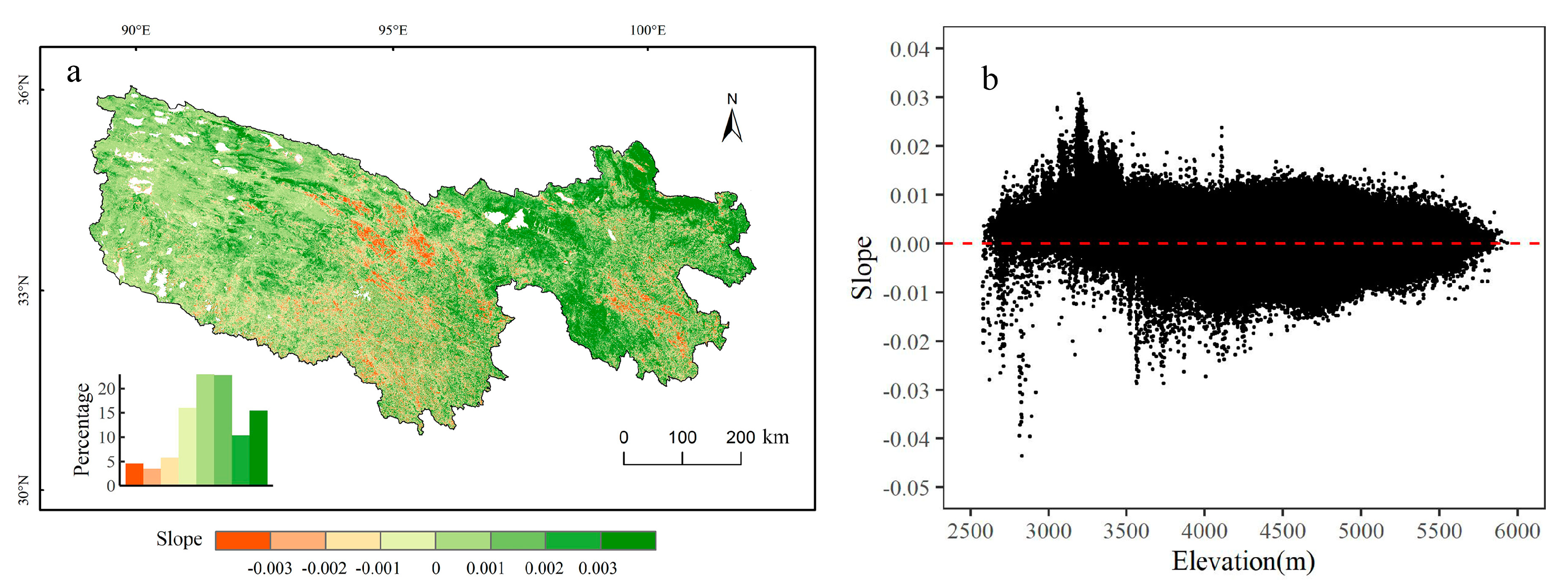
Trend analysis can comprehensively reflect the spatiotemporal change characteristics of vegetation growth in the study area, and the vegetation growth trend of the TRHR over the past 20 years was calculated using the method of linear regression analysis. The results revealed that the area of improved vegetation (Slope > 0) was much larger than the area of degraded vegetation (Slope < 0) during 2000–2021 (Figure 4a). The area of improvement was 236,803.38 km2, accounting for 74.77% of the total area, and the area of degradation was 103,474.31 km2, accounting for 25.23% of the total area. The areas with a significant trend of improvement (Slope > 0.003) were mainly distributed in the northeast and southeast of the TRHR, and areas with a significant trend of degradation (Slope < −0.003) were mainly distributed in the central part of the TRHR. With changing elevation, the trend of vegetation growth also showed significant differences. At elevations below 3500 m above sea level, the vegetation growth trend mainly showed significant improvement, which might be related to ecological management measures and the development of more suitable climatic conditions in recent years. With the increase in elevation, the impact of anthropogenic disturbance gradually decreases, and the climatic conditions tend to be more stable; thus, the slope of the EVI gradually decreases and the trend of vegetation growth is less obvious (Figure 4b).

4.2.2. Vegetation Growth Volatility

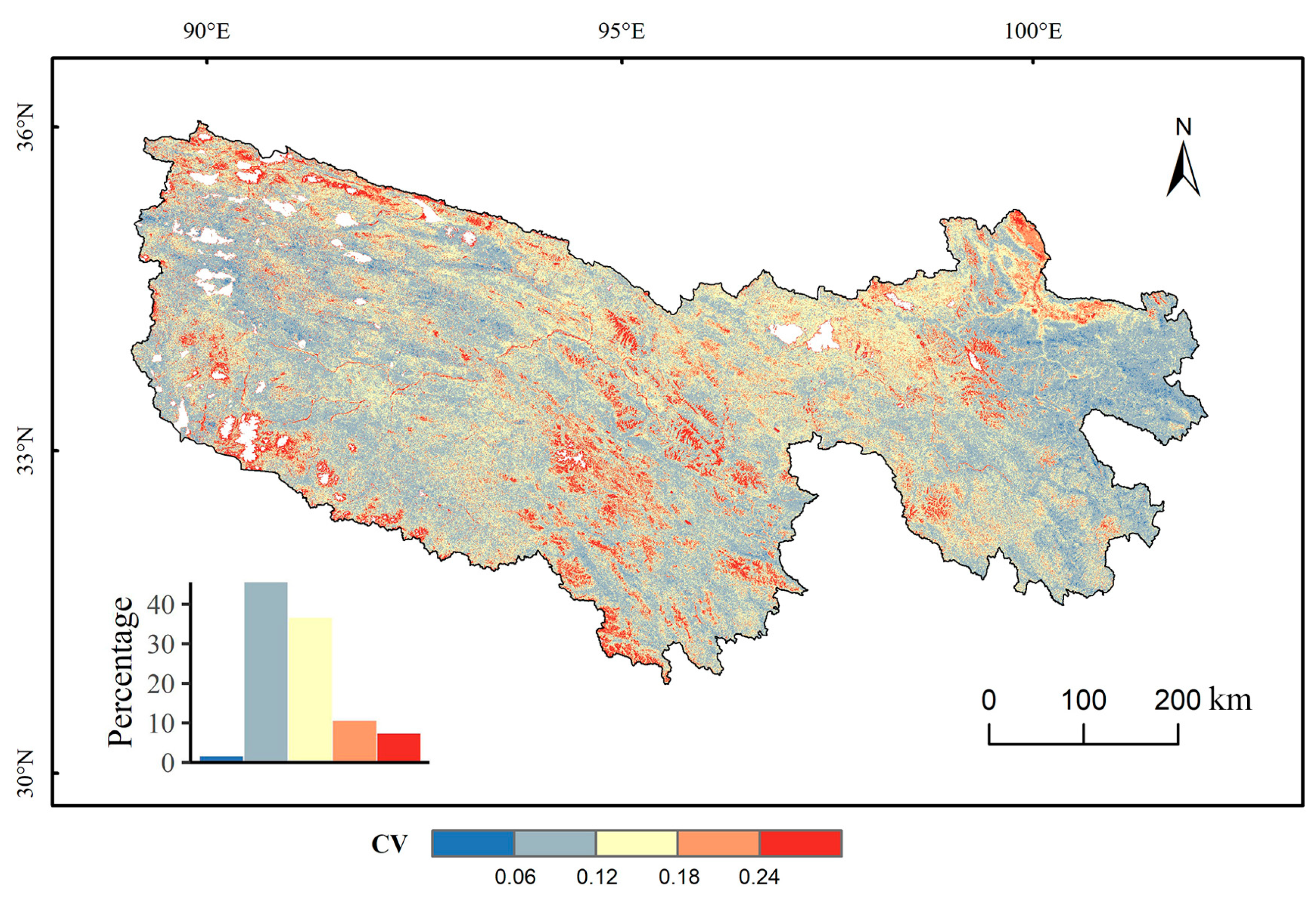
To enhance the comparability of the maximum annual fluctuation of the EVI at different spatial scales, the CV was used as the fluctuation evaluation index to quantitatively evaluate the degree of ΔEVI variability in the TRHR. The EVI time series spectra of the TRHR area during 2000–2021 were calculated and processed to obtain the CV spatial distribution (Figure 5). Analysis showed that the CV of ΔEVI in the TRHR during 2000–2021 was mainly concentrated between 0.06 and 0.18, with a peak located at 0.1017. The areas with CV values in the range of 0 ≤ CV < 0.06, 0.06 ≤ CV < 0.18, 0.12 ≤ CV < 0.18, 0.18 ≤ CV < 0.24, and CV ≥ 0.24 accounted for 1.15%, 45.55%, 36.19%, 10.19%, and 6.92% of the total area of the region, respectively. Of these, the area with CV values in the range 0.06 ≤ CV < 0.18 represents the largest proportion of fluctuating vegetation in the TRHR, representing 81.74% of the study area, mainly distributed in the western and southeastern areas.

4.2.3. EEMD Trends of Vegetation Growth

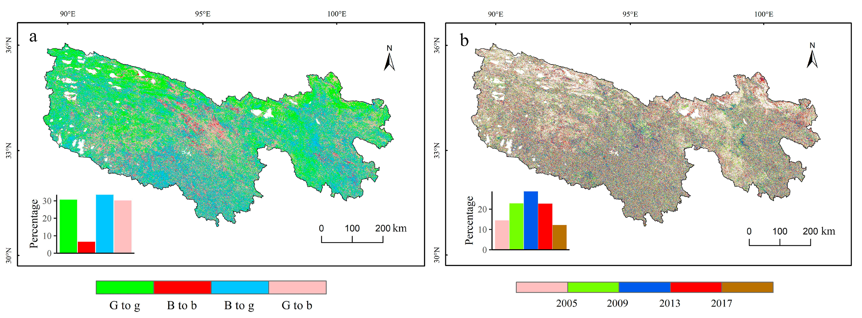
In terms of long-term trends, the spatial distribution of the EEMD secular trends of the EVI was similar to that determined using linear regression analysis, with 63.79% and 36.21% vegetation improvement and vegetation degradation, respectively. This indicates that in the past 20 years, most areas of the TRHR have shown a greening trend, with vegetation improvement areas mainly in the northern and southern parts of the Yellow River source area and western parts of the Yangtze River source area. The vegetation degradation areas are mainly in the central parts of the Yellow River source area, western parts of the Yangtze River source area, and most of the Lancang River source area. However, unlike linear regression analysis, in addition to determining the monotonic change trend of vegetation, the EEMD method can detect the trend variations of vegetation from greening-to-browning and from browning-to-greening. As can be seen in Figure 6a, areas with monotonically greening vegetation accounted for 30.30% of the total area (i.e., 44.47% less than that detected using linear regression analysis) and the percentage of areas with monotonically browning vegetation was 6.30%. Trend conversion occurred in 63.40% of the areas, among which 33.49% of the areas had browning-to-greening reversals, mainly concentrated in the eastern and southern parts of the TRHR, and 29.91% of the areas had greening-to-browning reversals, mainly concentrated in the central parts of the TRHR. The change points of the EVI trend mainly occurred after 2005 (Figure 6b), which might be related to anthropogenic activities in 2005 and the influence of climate change. In addition to the changes in climatic factors, the first phase of the TRHR Ecological Protection and Construction Project was officially launched in 2005; it introduced many measures such as grazing and grass restoration, ecological migration, and artificial rainfall with the aim of fully restoring the ecological environment of the TRHR. The implementation of active ecological management measures evidently had an important impact on the change in EVI growth trends.

4.2.4. Prediction of Future Vegetation Trends

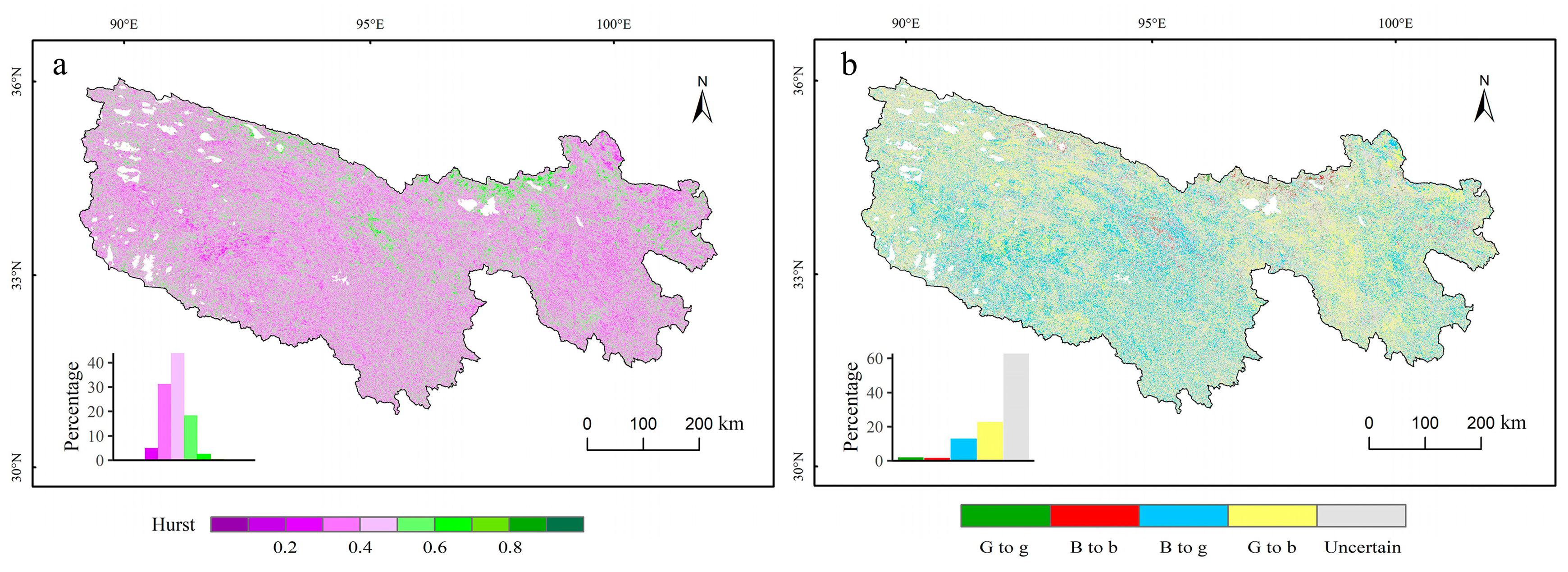
The Hurst exponent was used to predict the vegetation growth trend in the TRHR, and the results showed that the Hurst index (H) value of the EVI in the TRHR area was in the range of 0.0061–0.9543 (mean value: 0.4349), in which the number of pixels with a value of H < 0.5 accounted for 79.57%; this indicated that the inverse feature of vegetation change in the TRHR area was stronger than the isotropic feature. However, 62.79% of the pixels had H values of 0.4–0.6, which means that their future EVI trends are uncertain. Pixels with strong consistent trends (H > 0.6) and strong reverse trends (H < 0.4) accounted for 2.60% and 34.61% of the total area, respectively.
On the basis of the trend of the EEMD method and the Hurst exponent, we constructed a grading system for future prediction of the vegetation growth trend in the TRHR (Table 1) and calculated the future trend characteristics of vegetation growth change in the TRHR (Figure 7). The area of future continuous vegetation improvement and the area of future continuous vegetation degradation in the TRHR area accounted for 1.46% and 1.15% of the total area, respectively. The area of future browning-to-greening vegetation accounted for 12.36% of the total area. The area of future greening-to-browning vegetation accounted for 22.24% of the total area. The area showing a random trend, indicating an unclear future change in vegetation, accounted for 62.79% of the area. The area of future vegetation degradation in the TRHR was larger than the area of future vegetation improvement, and the risk of vegetation degradation is higher.

4.3. Climatic Effects of Vegetation Growth

4.3.1. Changes in Climatic Factors

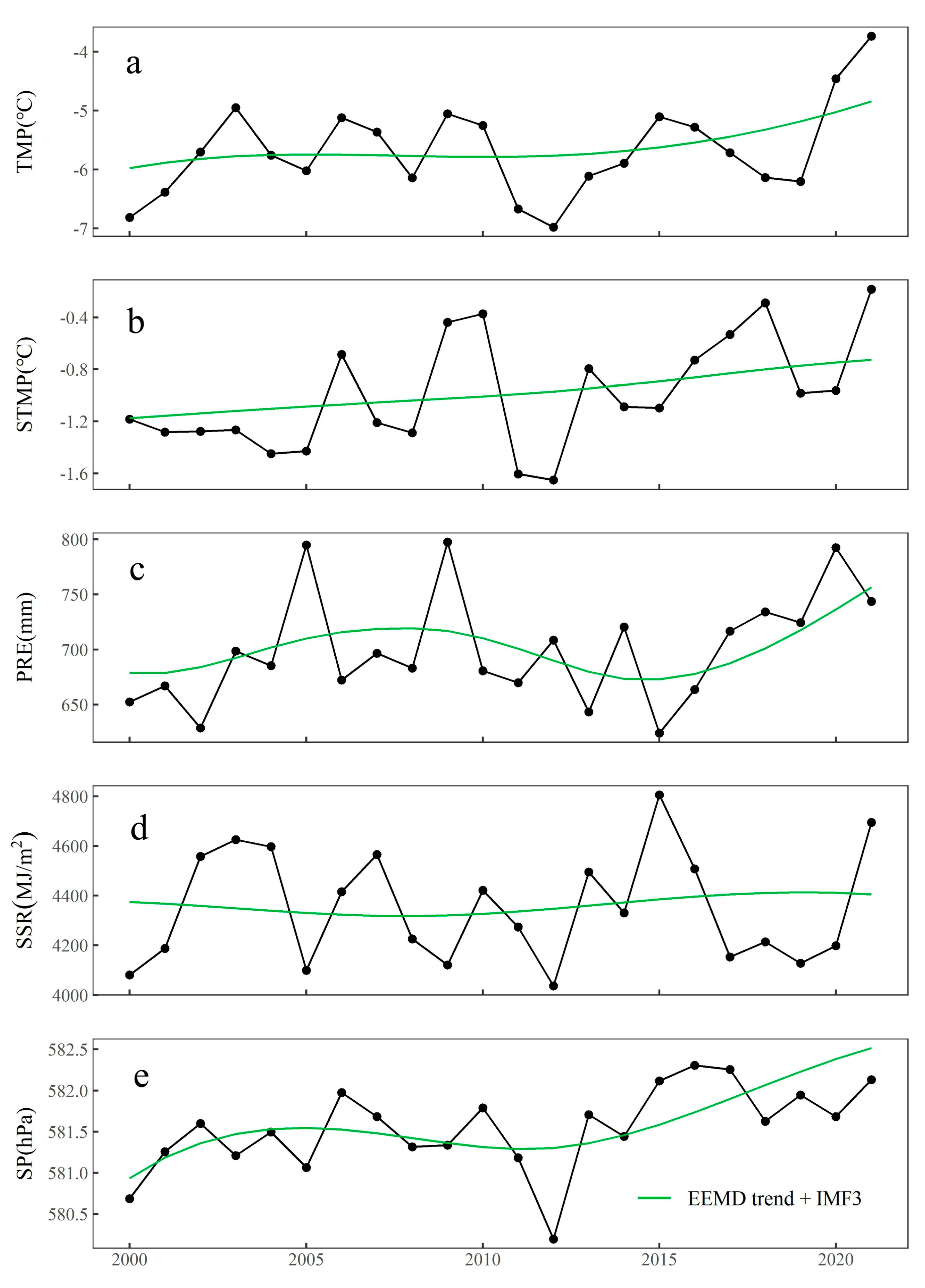
In addition to the role of soil fertility, changes in vegetation growth are more often influenced by a combination of hydrological and thermal factors [38]. To analyze the climatic effects of vegetation growth in the TRHR during 2000–2021, the changes in TMP, STMP, PRE, SP, and SSR during the same period were statistically analyzed separately (Figure 8). The results revealed that the annual average value of TMP was −5.68 °C, which is influenced by global warming, and the temperature of the TRHR has been increasing slowly over the past 20 years. The annual average value of STMP was −0.99 °C, which was relatively stable before 2006, but then, fluctuated slightly thereafter. The topography of the TRHR is complex, and the warm and humid airflow is blocked by high mountains, which results in low precipitation in the TRHR, that is, the annual average precipitation is 700.01 mm. Owing to the high elevation and plateau’s high pressure, the TRHR has thin air, long sunshine duration, and strong solar radiation, with an annual average SSR of 4351.70 MJ/m2 and an annual average SP of 581.54 hPa.
Sudden changes in climate could have a major impact on the growth status of vegetation. Before 2005, temperature and precipitation both showed a slow upward trend, with gradual improvement in the climatic conditions suitable for vegetation growth, and the EVI increased. However, in 2006, the TRHR suffered a severe drought with recorded precipitation of 27.68 mm less than the annual average, which reduced crop yields on a large scale and threatened the regional grassland ecology. This trend continued until 2008 and the EVI also showed a decreasing trend during 2006–2008. The air temperature and soil temperature decreased significantly in 2011 and 2012, and the long-term low-temperature conditions inhibited vegetation growth and reduced plant photosynthesis. This effect could have a certain time lag, and the EVI also showed a decreasing trend during 2011–2015. However, after 2015, precipitation and soil temperature both gradually increased, and the improved hydrological and thermal conditions led to markedly improved vegetation growth and a gradual increase in the EVI.

4.3.2. Vegetation Response to Climate Change

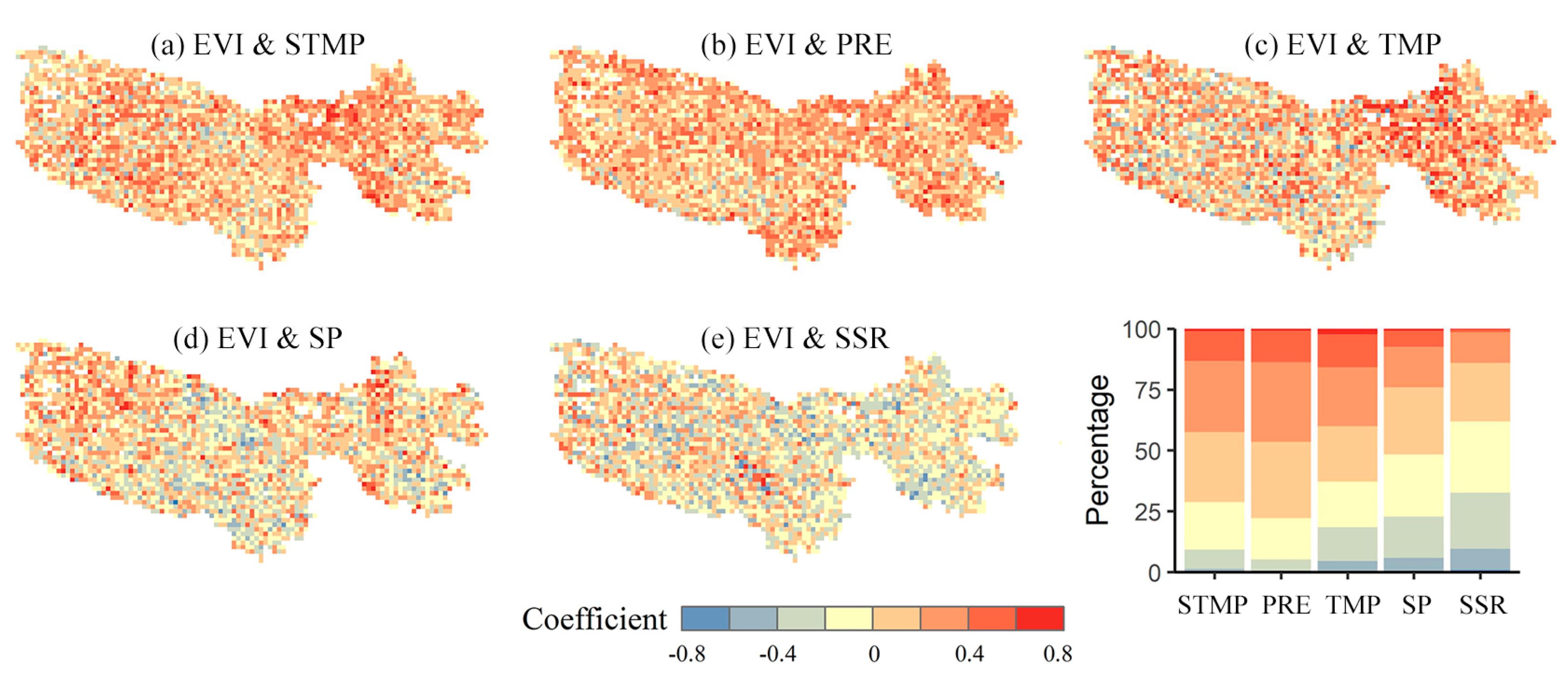
Owing to the complex topography of the TRHR and the great spatial heterogeneity of the regional climatic conditions, there is also strong spatial variability in the response of vegetation to climatic factors (Figure 9). During 2000–2021, the correlation analysis between PRE and the EVI showed that the areas with a positive correlation accounted for 77.84% of the study area and were mainly distributed in the northern and southern areas of the TRHR. Areas with a positive correlation between either STMP or TMP and the EVI accounted for 71.25% and 62.91% of the study area, respectively. In the area with a relatively high EVI in the central part of the TRHR, TMP and the EVI showed a strong correlation, while temperature gradually decreased with increasing elevation, and STMP became one of the main factors affecting vegetation growth. Areas with a negative correlation between SSR and the EVI accounted for 61.90% of the study area, indicating that radiation might have an inhibitory effect on vegetation growth, while areas with a strong negative correlation between SSR and the EVI were mainly in areas of vegetation improvement such as the southeastern part of the TRHR. The response of vegetation to SP showed strong spatial differences, with positive correlation pixels mainly distributed in eastern parts of the TRHR (51.70%) and negative correlation pixels mainly distributed in central and southeastern parts (48.30%).
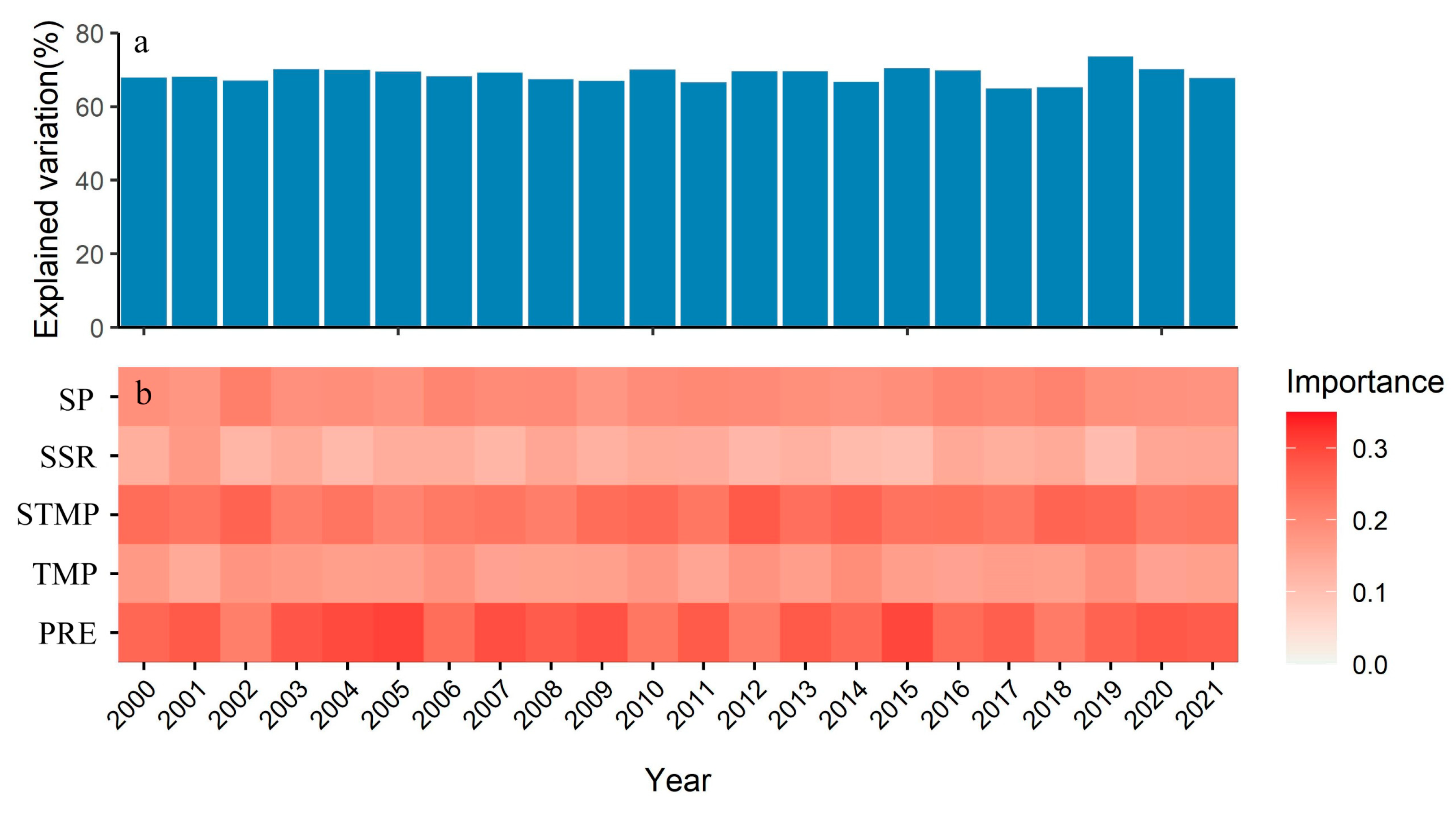
The RF model was used to analyze the spatial response of vegetation to climate. In the RF model, the coefficients of determination between simulated and real data were in the range of 0.6488–0.7355, with an average explained variation of 68.55% (Figure 10). The climatic factors clearly explained the differences in the spatial distribution of vegetation and could satisfy the quantitative analysis of the drivers of vegetation change. The importance of independent variables derived from the RF model was used to indicate the contribution of predictors in controlling the EVI, while the importance was normalized. On the basis of the contribution of each climatic factor in the RF model, the influence of each of the climatic factors on vegetation growth in the TRHR during 2000–2021 was analyzed. PRE had the greatest influence on the spatial distribution of the EVI in the study area (average importance: 26.57%), and the second largest contribution came from STMP (average importance: 24.03%). However, the average importance of TMP was only 16.64%, which indicates that the spatial influence of TMP on vegetation distribution was much less than that of STMP, and the average importance of SP and SSR was 19.39% and 13.35%, respectively.

5. Discussion

5.1. Characteristics of Vegetation Change

The EVI of the TRHR during 2000–2021 shows an increasing trend. The Tibetan Climate Change Monitoring Bulletin shows that the average annual surface temperature in Tibet has increased by 0.31 °C/10a on average over the past half-century, and that the temperature in the TRHR in the hinterland of the Tibetan Plateau has increased by nearly 2 °C, with the average annual increase much higher than the global average. During 1961–2013, the average annual precipitation on the Tibetan Plateau showed an increasing trend, with an average increase of 6.8 mm/10a. Xu [39] reported that the vegetation in the TRHR showed a slight increase during 1982–2006, and this trend continued from 1982 to the present, indicating that the TRHR has experienced continuous greening in the past half-century.
The growth of vegetation is affected by a combination of anthropogenic and natural factors such as water and heat, and the hydrological and thermal conditions tend to vary widely from year to year. The occurrences of drought and extreme high temperature events will affect the vegetation growth status of the TRHR. During 2000–2021, 74.77% of the vegetation growth in the TRHR showed a trend of slow improvement, but some areas still had vegetation degradation. Areas with degradation were mainly distributed in and around the Lancang River source area, probably because such areas were affected by extreme weather such as drought from 2006 to 2008, which inhibited the growth of pasture in the TRHR, threatened the grassland ecology, and caused extensive damage to crops. In 2006, the average temperature of the Yushu Tibetan Autonomous Prefecture in the TRHR was 12.3 °C, which was 2.6 °C higher than the climatic average of the period from 1971 to 2000, making it the warmest year since 1961. In addition, human factors, such as population growth and overgrazing, were considered to be the main causes of grassland destruction [40,41]. Additionally, the activities of some soil-dwelling endemic small mammals might also accelerate local vegetation degradation [42].
On the other hand, active human policies and projects could improve local vegetation growth status. In 2005, China launched the Ecological Protection and Construction Project (EPCP) in the TRHR. Ecosystem degradation in the TRHR was initially contained and partially improved [43,44], there was a realistic livestock carrying capacity, and the grazing pressure index of grassland decreased significantly [45]. In the first EPCP phase (2005–2012), the areas of the newly increased and improved grassland in the TRHR were 123.70 km2 and 27260.53 km2, respectively, while the area of the desert ecosystem decreased by 492.61 km2. In the second phase (2013–2020), the area of improved grassland was 6572.11 km2, and the area of desert ecosystems was reduced by 266.12 km2. With the implementation of the EPCP from 2005 to 2020, the forest and grassland coverage in the TRHR increased from 4.8% to 7.43% and from 73% to 75%, respectively. In general, the increase in vegetation coverage and the decrease in desert ecosystem area have played a positive role in the improvement of the vegetation growth status in the TRHR. Meanwhile, climate change and artificial rainfall operations have resulted in increases in grassland net primary productivity and in the theoretical livestock carrying capacity [46]. The implementation of degraded grassland treatment in “black soil peach” and of rodent control was also conducive to the recovery of degraded grassland. The active ecological protection projects and policies, such as the Grain-to-Green Program, led some grassland to no longer assume an agricultural function. At the same time, the increase in precipitation, the restoration of vegetation, and wetland protection increased the water conservation capacity of the TRHR. Additionally, the areas of lakes and marshes showed a trend of expansion, with a significant increase in wildlife populations and the gradual recovery of biodiversity [47]. Owing to reduced interference from human activities, fluctuations in vegetation growth have stabilized in most areas of the TRHR, with only a few areas still experiencing large fluctuations in vegetation growth.
The traditional linear regression analysis method can only reveal changes in the monotonic trend of vegetation growth conditions while ignoring the trend transition of vegetation throughout the period, whereas the EEMD method can detect trend changes in vegetation growth from greening-to-browning and from browning-to-greening. Areas with monotonic greening of vegetation were found to account for 30.30% of the total area, which was 44.47% less than the area of monotonic greening detected using the linear regression analysis method. Moreover, most of the areas (63.40%) experienced trend transitions, which indicated that the vegetation change was not linear but complex and unstable. Meanwhile, the change point of the trend shift occurred mainly after 2005, which is consistent with the findings of Shen [48], and was mainly due to the implementation of policies aimed at restoring the ecological environment of the TRHR and promoting vegetation improvement in this year, as well as the large abrupt changes in climatic factors after 2005.
Notably, the results of the Hurst exponent indicate that 62.79% of the areas show a stochastic nature of future vegetation changes and 23.39% of the areas might undergo degradation in the future, a large portion of which is from improvements to degradation. However, the Hurst exponent relies only on a single calculation of the vegetation time series, and vegetation growth is often influenced by multiple factors. Therefore, the Hurst exponent does not provide a definite time for the prediction of vegetation, but instead, represents more of a risk indication [14]. However, this risk indication is an important reference value for guiding ecological conservation and restoration in the TRHR.

5.2. Climate Response of Vegetation Growth

In arid and semiarid zones where water resources are relatively scarce, precipitation is a key factor affecting vegetation growth [49,50]. At the same time, low temperature is also one of the main factors limiting growth at high elevations [51], and climate warming can substantially promote the growth of highland vegetation [52]. Most previous studies suggest that temperature is the main driver of vegetation improvement in the TRHR [15,27,53]; however, some studies have found that precipitation has a greater effect on vegetation growth in the TRHR [29]. The inconsistency between these results might be attributable to differences in spatiotemporal models of the effects of climate on plant growth, and the response of different vegetation types to climate change might vary depending on differences in root morphology and the dominant vegetation species. Zhai [16] reported that alpine meadow and grassland vegetation in the TRHR are more sensitive to precipitation, and that alpine shrubs respond more to temperature than to precipitation.
In the temporal model, the positive response of vegetation to PRE occurred in most areas of the TRHR, and the negative response was mainly distributed in the areas of degraded vegetation in the southwest. In the area of high vegetation coverage in the central TRHR, TMP showed a strong positive correlation with vegetation, probably because alpine shrubs are more sensitive to temperature [54]. As elevation increases, the importance of STMP becomes increasingly apparent. The main vegetation types in the central and eastern parts of the TRHR are sparse grassland and alpine meadow, and their root systems are mostly distributed in the soil at a depth of approximately 10 cm. STMP will have a direct effect on the root systems of such vegetation, and because permafrost is widespread in the TRHR, higher soil temperatures will promote melting of the permafrost [55], which indirectly promotes vegetation growth. Yang [56] concluded that ground temperature is the main influencing factor of vegetation growth in the Yellow River and Yangtze River source areas. Xu [39] also suggested that soil temperature might make a more important contribution to vegetation change, and our results corroborate the above studies. A certain level of solar radiation can promote photosynthesis; however, excessive radiation might exceed the light saturation point of plants, limiting photosynthesis and causing water evaporation, which inhibits vegetation growth. Figure 8 and Figure 9 show that the reduction in SSR over the past 20 years has effectively alleviated such inhibitory effects on vegetation growth in the TRHR.
In the spatial model, these five climate factors can thoroughly explain the regional differences in the EVI, and precipitation is considered to be the main climatic factor controlling the spatial differences in vegetation growth. This is probably because, at the regional scale, an increase in precipitation can stimulate the accumulation of vegetation carbon [57] and influence the growing season of vegetation [58], and precipitation is also a key determinant of spatial changes in soil organic carbon stocks and microbial properties on the QTP [59,60]. Li [61] also found that precipitation plays the most important role in the variation of soil respiration in the growing and non-growing seasons in the permafrost zone of the QTP.

5.3. Effect of Elevation on Vegetation Growth

The distribution of vegetation is closely related to the elevation gradient [62], and elevation indirectly controls the growth of vegetation by influencing climatic factors such as temperature and precipitation [63]. The results showed that the EVI and Slope in the TRHR increased, and then, decreased with elevation, that the EVI peaked at the elevation of 3500–4000 m, and that the vegetation changed most drastically at the elevation of 3000–3500 m (Table 2). The main reason is that anthropogenic activities are more intense and widespread at lower elevations, and the development of cities and the opening up of agricultural land have great impacts on vegetation growth. With increasing elevation, temperature and precipitation both gradually decrease, and the vegetation type changes from scrub and alpine meadow with higher EVI values to alpine grassland and sparse grassland with lower EVI values to adapt to the low-temperature climate. However, the CV values show the same trend as elevation, which might reflect that the CV is more influenced by the mean value.

6. Conclusions

This study synthesized the spatiotemporal characteristics of vegetation growth in the TRHR and investigated the trends and responses of vegetation growth to climate since the beginning of the 21st century. The results of the linear regression analysis of the time series EVI showed that two-thirds of the regional vegetation in the TRHR showed a greening trend, and that the vegetation was dominated by mild and moderate fluctuations. The EEMD method detected a trend shift in 63.40% of the area, and 85.91% of the trend shifts occurred after 2005. There were significant spatial differences in the response of vegetation growth to climatic changes in the TRHR. The increase in precipitation substantially promoted vegetation growth in the TRHR, the increase in both ground temperature and air temperature also led to the improvement of vegetation growth, and the decrease in radiation alleviated the inhibitory effect on vegetation growth. The results of the spatial model indicate that precipitation is the most important driver of vegetation growth in the TRHR. However, the investigation of future vegetation dynamics based on the Hurst exponent showed that the area of degraded vegetation in the TRHR might be larger than the area of improved vegetation, and that the risk of vegetation degradation is higher. To reduce the risk of ecological degradation in the TRHR, based on the construction of the TRHR National Park, a series of measures are needed to protect the ecological environment in and around the TRHR, to explore the model of harmonious coexistence between humans and nature, to improve awareness and the participation of local people in ecological environmental protection, and to support ecological restoration and protection in the TRHR.

Author Contributions

Conceptualization, F.Y.; Methodology, F.Y., Y.W. and C.H.; Software, C.H. and F.Y.; Validation, C.H., Y.W. and F.Y.; Formal Analysis, C.H., Y.W. and F.Y.; Investigation, C.H., Y.W. and F.Y.; Resources, Y.W., F.Y., Q.L. and C.H.; Data Curation, Y.W. and C.H.; Writing—Original Draft Preparation, C.H., Y.W. and F.Y.; Writing—Review and Editing, F.Y., C.H. and Q.L.; Visualization, C.H. and Y.W.; Supervision, F.Y. and Q.L.; Project Administration, F.Y.; Funding Acquisition, F.Y. All authors have read and agreed to the published version of the manuscript.

Funding

This research was funded by the National Nonprofit Institute Research Grant of the Chinese Academy of Forestry (grant numbers CAFYBB2019GB001 and CAFYBB2018ZA004), the Fengyun Application Pioneering Project (grant number FY-APP-2021.0402) and National Science Foundation of China (grant number 41301458).

Acknowledgments

The authors would like to thank NASA for sharing their MODIS data and DEM data, the Copernicus Climate Change Service for sharing their climate data, and the Data Sharing and Service Portal of the Chinese Academy of Sciences for sharing their land cover type data.

Conflicts of Interest

The authors declare no conflict of interest.

References

  1. Sun, W.; Song, X.; Mu, X.; Gao, P.; Wang, F.; Zhao, G. Spatiotemporal Vegetation Cover Variations Associated with Climate Change and Ecological Restoration in the Loess Plateau. Agric. For. Meteorol. 2015, 209, 87–99. [Google Scholar] [CrossRef]
  2. Gao, M.; Wang, X.; Meng, F.; Liu, Q.; Li, X.; Zhang, Y.; Piao, S. Three-dimensional Change in Temperature Sensitivity of Northern Vegetation Phenology. Glob. Change Biol. 2020, 26, 5189–5201. [Google Scholar] [CrossRef]
  3. Lian, X.; Jiao, L.; Liu, Z.; Jia, Q.; Zhong, J.; Fang, M.; Wang, W. Multi-Spatiotemporal Heterogeneous Legacy Effects of Climate on Terrestrial Vegetation Dynamics in China. Gisci. Remote Sens. 2022, 59, 164–183. [Google Scholar] [CrossRef]
  4. Nemani, R.R.; Keeling, C.D.; Hashimoto, H.; Jolly, W.M.; Piper, S.C.; Tucker, C.J.; Myneni, R.B.; Running, S.W. Climate-Driven Increases in Global Terrestrial Net Primary Production from 1982 to 1999. Science 2003, 300, 1560–1563. [Google Scholar] [CrossRef] [Green Version]
  5. Bonan, G.B. Forests and Climate Change: Forcings, Feedbacks, and the Climate Benefits of Forests. Science 2008, 320, 1444–1449. [Google Scholar] [CrossRef] [PubMed] [Green Version]
  6. Ma, Y.; Guan, Q.; Sun, Y.; Zhang, J.; Yang, L.; Yang, E.; Li, H.; Du, Q. Three-Dimensional Dynamic Characteristics of Vegetation and Its Response to Climatic Factors in the Qilian Mountains. Catena 2022, 208, 105694. [Google Scholar] [CrossRef]
  7. IPCC. Climate change 2021: The physical science basis [M/OL]. 2021 [2021-08-22]. Available online: https://www.ipcc.ch/report/ar6/wg1/ (accessed on 15 December 2021).
  8. Zhou, L.; Tian, Y.; Myneni, R.B.; Ciais, P.; Saatchi, S.; Liu, Y.Y.; Piao, S.; Chen, H.; Vermote, E.F.; Song, C.; et al. Widespread Decline of Congo Rainforest Greenness in the Past Decade. Nature 2014, 509, 86–90. [Google Scholar] [CrossRef] [PubMed]
  9. Xie, Y.; Wang, X.; Wilson, A.M.; Silander, J.A. Predicting Autumn Phenology: How Deciduous Tree Species Respond to Weather Stressors. Agric. For. Meteorol. 2018, 250, 127–137. [Google Scholar] [CrossRef]
  10. Qiu, T.; Song, C.; Clark, J.S.; Seyednasrollah, B.; Rathnayaka, N.; Li, J. Understanding the Continuous Phenological Development at Daily Time Step with a Bayesian Hierarchical Space-Time Model: Impacts of Climate Change and Extreme Weather Events. Remote Sens. Environ. 2020, 247, 111956. [Google Scholar] [CrossRef]
  11. Huete, A.; Didan, K.; Miura, T.; Rodriguez, E.P.; Gao, X.; Ferreira, L.G. Overview of the Radiometric and Biophysical Performance of the MODIS Vegetation Indices. Remote Sens. Environ. 2002, 83, 195–213. [Google Scholar] [CrossRef]
  12. Yan, F.; Wu, B.; Wang, Y. Estimating Spatiotemporal Patterns of Aboveground Biomass Using Landsat TM and MODIS Images in the Mu Us Sandy Land, China. Agric. For. Meteorol. 2015, 200, 119–128. [Google Scholar] [CrossRef]
  13. Peng, J.; Liu, Z.; Liu, Y.; Wu, J.; Han, Y. Trend Analysis of Vegetation Dynamics in Qinghai–Tibet Plateau Using Hurst Exponent. Ecol. Indic. 2012, 14, 28–39. [Google Scholar] [CrossRef]
  14. Chen, J.; Yan, F.; Lu, Q. Spatiotemporal Variation of Vegetation on the Qinghai–Tibet Plateau and the Influence of Climatic Factors and Human Activities on Vegetation Trend (2000–2019). Remote Sens. 2020, 12, 3150. [Google Scholar] [CrossRef]
  15. Bai, Y.; Guo, C.; Degen, A.A.; Ahmad, A.A.; Wang, W.; Zhang, T.; Li, W.; Ma, L.; Huang, M.; Zeng, H.; et al. Climate Warming Benefits Alpine Vegetation Growth in Three-River Headwater Region, China. Sci. Total Environ. 2020, 742, 140574. [Google Scholar] [CrossRef] [PubMed]
  16. Zhai, D.; Gao, X.; Li, B.; Yuan, Y.; Li, Y.; Liu, W.; Xu, J. Diverse Chronic Responses of Vegetation Aboveground Net Primary Productivity to Climatic Changes on Three-River Headwaters Region. Ecol. Indic. 2022, 139, 108925. [Google Scholar] [CrossRef]
  17. Gurung, R.B.; Breidt, F.J.; Dutin, A.; Ogle, S.M. Predicting Enhanced Vegetation Index (EVI) Curves for Ecosystem Modeling Applications. Remote Sens. Environ. 2009, 113, 2186–2193. [Google Scholar] [CrossRef]
  18. Pan, N.; Feng, X.; Fu, B.; Wang, S.; Ji, F.; Pan, S. Increasing Global Vegetation Browning Hidden in Overall Vegetation Greening: Insights from Time-Varying Trends. Remote Sens. Environ. 2018, 214, 59–72. [Google Scholar] [CrossRef]
  19. Wu, Z.; Huang, N.E. Ensemble Empirical Mode Decomposition: A Noise-Assisted Data Analysis Method. Adv. Adapt. Data Anal. 2009, 01, 1–41. [Google Scholar] [CrossRef]
  20. Ji, F.; Wu, Z.; Huang, J.; Chassignet, E.P. Evolution of Land Surface Air Temperature Trend. Nat. Clim. Change 2014, 4, 462–466. [Google Scholar] [CrossRef]
  21. Yin, Y.; Ma, D.; Wu, S.; Dai, E.; Zhu, Z.; Myneni, R.B. Nonlinear Variations of Forest Leaf Area Index over China during 1982–2010 Based on EEMD Method. Int. J. Biometeorol. 2017, 61, 977–988. [Google Scholar] [CrossRef]
  22. Xu, X.; Liu, H.; Jiao, F.; Gong, H.; Lin, Z. Time-Varying Trends of Vegetation Change and Their Driving Forces during 1981–2016 along the Silk Road Economic Belt. Catena 2020, 195, 104796. [Google Scholar] [CrossRef]
  23. Chen, D.; Xu, B.; Yao, T.; Guo, Z.; Cui, P.; Chen, F.; Zhang, R.; ZHANG, X.; ZHANG, Y.; FAN, J. Assessment of Past, Present and Future Environmental Changes on the Tibetan Plateau. Chin. Sci. Bull. 2015, 60, 3025–3035. [Google Scholar]
  24. Kuang, X.; Jiao, J.J. Review on Climate Change on the Tibetan Plateau during the Last Half Century. J. Geophys. Res. Atmos. 2016, 121, 3979–4007. [Google Scholar] [CrossRef] [Green Version]
  25. Diffenbaugh, N.S.; Field, C.B. Changes in Ecologically Critical Terrestrial Climate Conditions. Science 2013, 341, 486–492. [Google Scholar] [CrossRef] [Green Version]
  26. Sun, H.; Chen, Y.; Xiong, J.; Ye, C.; Yong, Z.; Wang, Y.; He, D.; Xu, S. Relationships between Climate Change, Phenology, Edaphic Factors, and Net Primary Productivity across the Tibetan Plateau. Int. J. Appl. Earth. Obs. 2022, 107, 102708. [Google Scholar] [CrossRef]
  27. Liu, X.; Zhang, J.; Zhu, X.; Pan, Y.; Liu, Y.; Zhang, D.; Lin, Z. Spatiotemporal Changes in Vegetation Coverage and Its Driving Factors in the Three-River Headwaters Region during 2000–2011. J. Geogr. Sci. 2014, 24, 288–302. [Google Scholar] [CrossRef]
  28. Yang, S.; Feng, Q.; Liang, T.; Liu, B.; Zhang, W.; Xie, H. Modeling Grassland Above-Ground Biomass Based on Artificial Neural Network and Remote Sensing in the Three-River Headwaters Region. Remote Sens. Environ. 2018, 204, 448–455. [Google Scholar] [CrossRef]
  29. Zheng, Y.; Han, J.; Huang, Y.; Fassnacht, S.R.; Xie, S.; Lv, E.; Chen, M. Vegetation Response to Climate Conditions Based on NDVI Simulations Using Stepwise Cluster Analysis for the Three-River Headwaters Region of China. Ecol. Indic. 2018, 92, 18–29. [Google Scholar] [CrossRef]
  30. Luukko, P.J.J.; Helske, J.; Räsänen, E. Introducing Libeemd: A Program Package for Performing the Ensemble Empirical Mode Decomposition. Computation. Stat. 2016, 31, 545–557. [Google Scholar] [CrossRef] [Green Version]
  31. Hurst, H.E. Long-Term Storage Capacity of Reservoirs. Trans. Am. Soc. Civ. Eng. 1951, 116, 770–799. [Google Scholar] [CrossRef]
  32. John, R.; Chen, J.; Lu, N.; Guo, K.; Liang, C.; Wei, Y.; Asko, N.; Ma, K.; Han, K. Predicting Plant Diversity Based on Remote Sensing Products in the Semi-Arid Region of Inner Mongolia. Remote Sens. Environ. 2008, 112, 2018–2032. [Google Scholar] [CrossRef]
  33. Jiang, L.; Jiapaer, G.; Bao, A.; Guo, H.; Ndayisaba, F. Vegetation Dynamics and Responses to Climate Change and Human Activities in Central Asia. Sci. Total Environ. 2017, 599, 967–980. [Google Scholar] [CrossRef] [PubMed]
  34. Breiman, L. Random Forests. Mach Learn 2001, 45, 5–32. [Google Scholar] [CrossRef] [Green Version]
  35. Franke, A.K.; Feilhauer, H.; Bräuning, A.; Rautio, P.; Braun, M. Remotely Sensed Estimation of Vegetation Shifts in the Polar and Alpine Tree-Line Ecotone in Finnish Lapland during the Last Three Decades. For. Ecol. Manag. 2019, 454, 117668. [Google Scholar] [CrossRef]
  36. Assal, T.J.; Steen, V.A.; Caltrider, T.; Cundy, T.; Stewart, C.; Manning, N.; Anderson, P.J. Monitoring Long-Term Riparian Vegetation Trends to Inform Local Habitat Management in a Mountainous Environment. Ecol. Indic. 2021, 127, 107807. [Google Scholar] [CrossRef]
  37. Liaw, A.; Wiener, M. Classification and Regression by RandomForest. R News 2002, 2, 5. [Google Scholar]
  38. Qiu, T.; Andrus, R.; Aravena, M.-C.; Ascoli, D.; Bergeron, Y.; Berretti, R.; Berveiller, D.; Bogdziewicz, M.; Boivin, T.; Bonal, R.; et al. Limits to Reproduction and Seed Size-Number Trade-Offs That Shape Forest Dominance and Future Recovery. Nat. Commun. 2022, 13, 2381. [Google Scholar] [CrossRef] [PubMed]
  39. Xu, W.; Gu, S.; Zhao, X.; Xiao, J.; Tang, Y.; Fang, J.; Zhang, J.; Jiang, S. High Positive Correlation between Soil Temperature and NDVI from 1982 to 2006 in Alpine Meadow of the Three-River Source Region on the Qinghai-Tibetan Plateau. Int. J. Appl. Earth. Obs. 2011, 13, 528–535. [Google Scholar] [CrossRef]
  40. Li, X.-L.; Gao, J.; Brierley, G.; Qiao, Y.-M.; Zhang, J.; Yang, Y.-W. Rangeland Degradation on the Qinghai-Tibet Plateau: Implications for Rehabilitation. Land Degrad. Dev. 2013, 24, 72–80. [Google Scholar] [CrossRef]
  41. Mipam, T.-D.; Zhong, L.-L.; Liu, J.-Q.; Miehe, G.; Tian, L.-M. Productive Overcompensation of Alpine Meadows in Response to Yak Grazing in the Eastern Qinghai-Tibet Plateau. Front. Plant Sci. 2019, 10, 925. [Google Scholar] [CrossRef] [Green Version]
  42. Miehe, G.; Schleuss, P.-M.; Seeber, E.; Babel, W.; Biermann, T.; Braendle, M.; Chen, F.; Coners, H.; Foken, T.; Gerken, T.; et al. The Kobresia Pygmaea Ecosystem of the Tibetan Highlands—Origin, Functioning and Degradation of the World’s Largest Pastoral Alpine Ecosystem. Sci. Total Environ. 2019, 648, 754–771. [Google Scholar] [CrossRef] [PubMed]
  43. Lu, Q.; Ning, J.; Liang, F.; Bi, X. Evaluating the Effects of Government Policy and Drought from 1984 to 2009 on Rangeland in the Three Rivers Source Region of the Qinghai-Tibet Plateau. Sustainability 2017, 9, 1033. [Google Scholar] [CrossRef]
  44. Shao, Q.; Cao, W.; Fan, J.; Huang, L.; Xu, X. Effects of an Ecological Conservation and Restoration Project in the Three-River Source Region, China. J. Geogr. Sci. 2017, 27, 183–204. [Google Scholar] [CrossRef]
  45. Zhang, L.; Fan, J.; Zhou, D.; Zhang, H. Ecological Protection and Restoration Program Reduced Grazing Pressure in the Three-River Headwaters Region, China. Rangel. Ecol. Manag. 2017, 70, 540–548. [Google Scholar] [CrossRef]
  46. Chen, H.; Ju, P.; Zhang, J.; Wang, Y.; Zhu, Q.; Yan, L.; Kang, X.; He, Y.; Zeng, Y.; Hao, Y.; et al. Attribution Analyses of Changes in Alpine Grasslands on the Qinghai-Tibetan Plateau. Chin. Sci. Bull. 2020, 65, 2406–2418. [Google Scholar] [CrossRef]
  47. Shao, Q.; Fan, J.; Liu, J.; Huang, L.; Cao, W.; Liu, L. Target-Based Assessment on Effects of First-Stage Ecological Conservation and Restoration Project in Three-River Source Region, China and Policy Recommendations. Bull. Chin. Acad. Sci. 2017, 32, 35–44. [Google Scholar]
  48. Shen, X.; An, R.; Li, F.; Nan, Y.; Zhu, L.; Li, M. Vegetation Changes in the Three-River Headwaters Region of the Tibetan Plateau of China. Ecol. Indic. 2018, 93, 804–812. [Google Scholar] [CrossRef]
  49. Fabricante, I.; Oesterheld, M.; Paruelo, J.M. Annual and Seasonal Variation of NDVI Explained by Current and Previous Precipitation across Northern Patagonia. J. Arid. Environ. 2009, 73, 745–753. [Google Scholar] [CrossRef]
  50. Wang, J.; Wang, K.; Zhang, M.; Zhang, C. Impacts of Climate Change and Human Activities on Vegetation Cover in Hilly Southern China. Ecol. Eng. 2015, 81, 451–461. [Google Scholar] [CrossRef]
  51. Li, L.; Zhang, Y.; Wu, J.; Li, S.; Zhang, B.; Zu, J.; Zhang, H.; Ding, M.; Paudel, B. Increasing Sensitivity of Alpine Grasslands to Climate Variability along an Elevational Gradient on the Qinghai-Tibet Plateau. Sci. Total Environ. 2019, 678, 21–29. [Google Scholar] [CrossRef] [PubMed]
  52. Lehnert, L.W.; Wesche, K.; Trachte, K.; Reudenbach, C.; Bendix, J. Climate Variability Rather than Overstocking Causes Recent Large Scale Cover Changes of Tibetan Pastures. Sci. Rep-UK 2016, 6, 24367. [Google Scholar] [CrossRef] [PubMed] [Green Version]
  53. Chen, C.; Li, T.; Sivakumar, B.; Li, J.; Wang, G. Attribution of Growing Season Vegetation Activity to Climate Change and Human Activities in the Three-River Headwaters Region, China. J. Hydroinform 2020, 22, 186–204. [Google Scholar] [CrossRef] [Green Version]
  54. Martin, A.C.; Jeffers, E.S.; Petrokofsky, G.; Myers-Smith, I.; Macias-Fauria, M. Shrub Growth and Expansion in the Arctic Tundra: An Assessment of Controlling Factors Using an Evidence-Based Approach. Environ. Res. Lett. 2017, 12, 085007. [Google Scholar] [CrossRef]
  55. Gu, S.; Tang, Y.; Cui, X.; Kato, T.; Du, M.; Li, Y.; Zhao, X. Energy Exchange between the Atmosphere and a Meadow Ecosystem on the Qinghai–Tibetan Plateau. Agric. For. Meteorol. 2005, 129, 175–185. [Google Scholar] [CrossRef]
  56. Yang, J.; Ding, Y.; Chen, R. Spatial and Temporal of Variations of Alpine Vegetation Cover in the Source Regions of the Yangtze and Yellow Rivers of the Tibetan Plateau from 1982 to 2001. Environ. Geol. 2006, 50, 313–322. [Google Scholar] [CrossRef]
  57. Yang, Y.H.; Fang, J.Y.; Pan, Y.D.; Ji, C.J. Aboveground Biomass in Tibetan Grasslands. J. Arid. Environ. 2009, 73, 91–95. [Google Scholar] [CrossRef]
  58. Liu, X.; Zhu, X.; Pan, Y.; Zhu, W.; Zhang, J.; Zhang, D. Thermal Growing Season and Response of Alpine Grassland to Climate Variability across the Three-Rivers Headwater Region, China. Agric. For. Meteorol. 2016, 220, 30–37. [Google Scholar] [CrossRef]
  59. Yang, Y.; Fang, J.; Tang, Y.; Ji, C.; Zheng, C.; He, J.; Zhu, B. Storage, Patterns and Controls of Soil Organic Carbon in the Tibetan Grasslands: SOIL ORGANIC CARBON IN TIBETAN GRASSLANDS. Glob. Change Biol. 2008, 14, 1592–1599. [Google Scholar] [CrossRef]
  60. Chen, Y.-L.; Ding, J.-Z.; Peng, Y.-F.; Li, F.; Yang, G.-B.; Liu, L.; Qin, S.-Q.; Fang, K.; Yang, Y.-H. Patterns and Drivers of Soil Microbial Communities in Tibetan Alpine and Global Terrestrial Ecosystems. J. Biogeogr. 2016, 43, 2027–2039. [Google Scholar] [CrossRef]
  61. Li, Q.; Liu, Y.; Kou, D.; Peng, Y.; Yang, Y. Substantial Non-growing Season Carbon Dioxide Loss across Tibetan Alpine Permafrost Region. Glob. Change Biol. 2022, 28, 5200–5210. [Google Scholar] [CrossRef]
  62. Piao, S.; Cui, M.; Chen, A.; Wang, X.; Ciais, P.; Liu, J.; Tang, Y. Altitude and Temperature Dependence of Change in the Spring Vegetation Green-up Date from 1982 to 2006 in the Qinghai-Xizang Plateau. Agric. For. Meteorol. 2011, 151, 1599–1608. [Google Scholar] [CrossRef]
  63. Liu, C.; Li, W.; Wang, W.; Zhou, H.; Liang, T.; Hou, F.; Xu, J.; Xue, P. Quantitative Spatial Analysis of Vegetation Dynamics and Potential Driving Factors in a Typical Alpine Region on the Northeastern Tibetan Plateau Using the Google Earth Engine. Catena 2021, 206, 105500. [Google Scholar] [CrossRef]
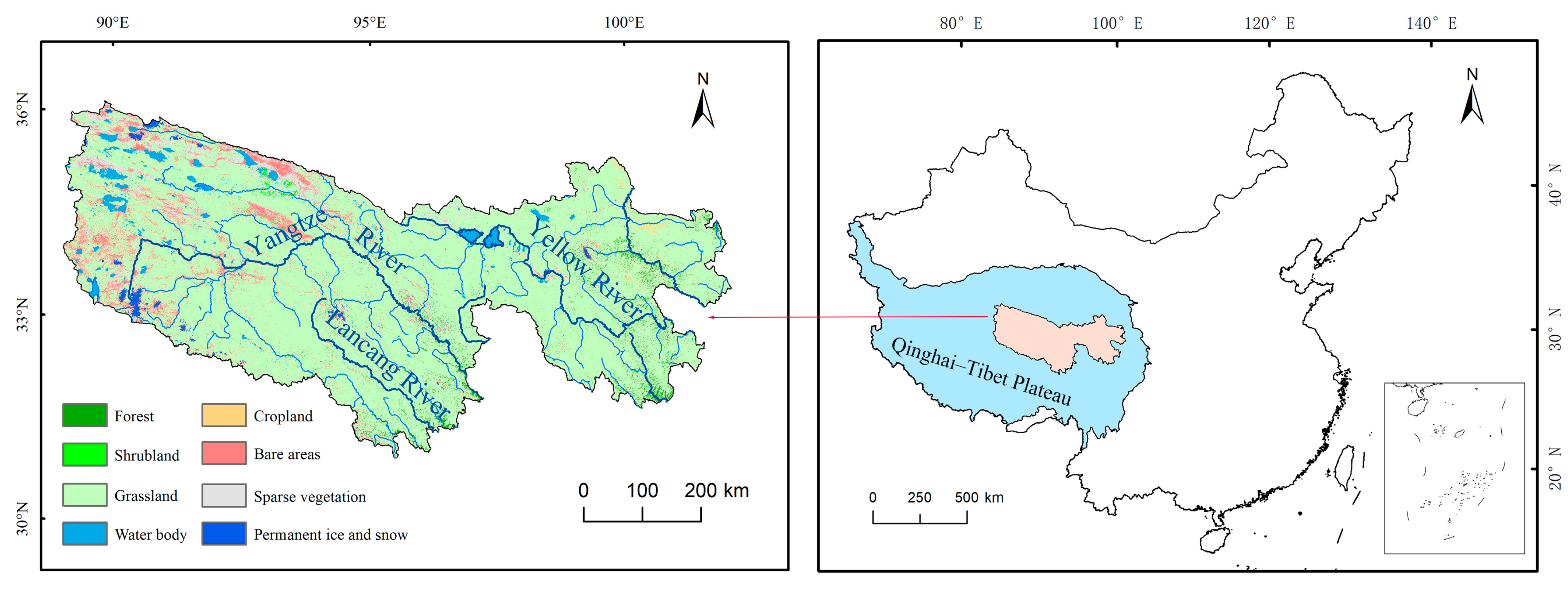
Figure 1. Location of the study area and the regional land use types.
Remotesensing 14 05041 g001
Figure 2. Variations in annual EVI (a) and interannual EVI (b) during 2000–2021.
Remotesensing 14 05041 g002
Figure 3. Distribution of annual mean EVI in the TRHR during 2000–2021: (a) spatially and (b) with elevation.
Remotesensing 14 05041 g003
Figure 4. Distribution of the EVI linear slope (a) and relation between slope and elevation (b) in the TRHR during 2000–2021.
Remotesensing 14 05041 g004
Figure 5. Spatial distribution of CV in the TRHR during 2000–2021.
Remotesensing 14 05041 g005
Figure 6. Spatial distributions of EVI trends (a) and the timing of change points derived using the EEMD method (b).
Remotesensing 14 05041 g006
Figure 7. Spatial distributions of the Hurst exponent (a) and future vegetation projections (b).
Remotesensing 14 05041 g007
Figure 8. Interannual variations in climatic factors (TMP (a), STMP(b), PRE(c), SSR(d), SP (e)) during 2000–2021.
Remotesensing 14 05041 g008
Figure 9. Spatial distributions of correlation analysis between the EVI and climatic factors (STMP (a), PRE (b), TMP (c), SP (d), SSR (e)).
Remotesensing 14 05041 g009
Figure 10. Importance evaluation based on the random forest model. The bar chart (a) shows the explanatory degree of the random forest regression model in the current year, and the colors (b) represent the importance.
Remotesensing 14 05041 g010
Table 1. Classification of EVI variation in the future.
EEMDH < 0.40.4 < H < 0.6H > 0.6
G TO G
B TO G
G TO BUncertainG TO G
B TO B
G TO B
B TO GUncertainB TO B
Table 2. Variation in vegetation growth status on the elevation gradient.
Elevation/mEVISlopeCV
2500–30000.2690 0.0029 0.1934
3000–35000.4155 0.0052 0.1591
3500–40000.5602 0.0019 0.0997
4000–45000.4196 0.0013 0.1241
4500–50000.2949 0.0008 0.1390
5000–55000.1686 0.0007 0.1787
5500–60000.0845 0.0005 0.3700
Publisher’s Note: MDPI stays neutral with regard to jurisdictional claims in published maps and institutional affiliations.