
Water Quality Retrieval from ZY1-02D Hyperspectral Imagery in Urban Water Bodies and Comparison with Sentinel-2


Abstract
1. Introduction
2. Materials and Methods
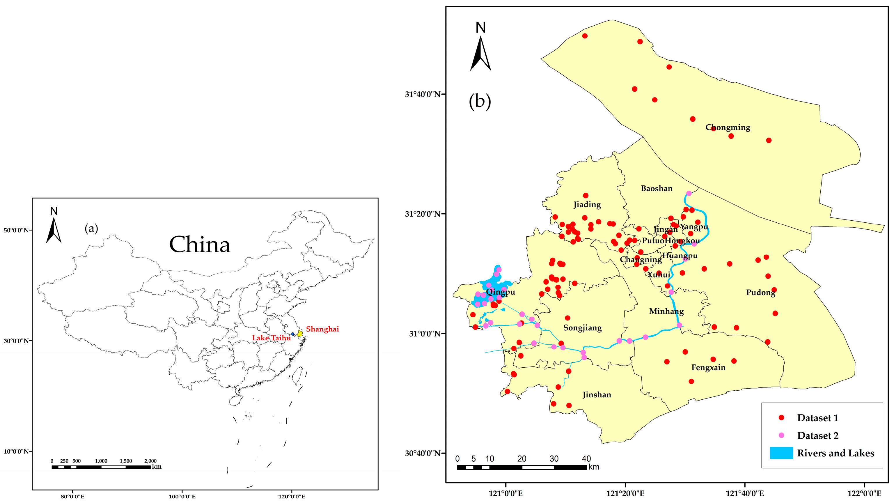
2.1. Study Area
2.2. Materials
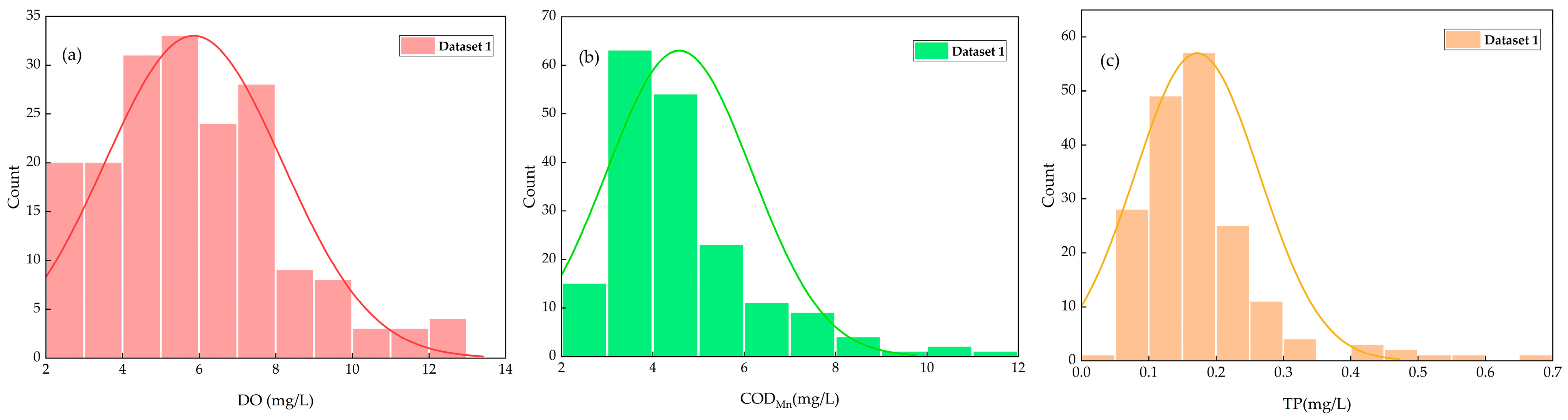
2.2.1. In Situ Data
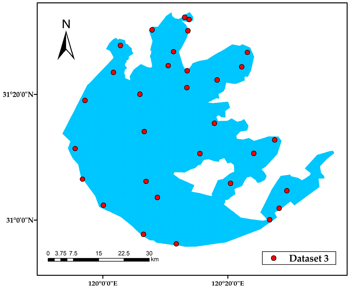
2.2.2. Independent Dataset in Taihu Lake
2.2.3. Satellite Data
2.3. Methods
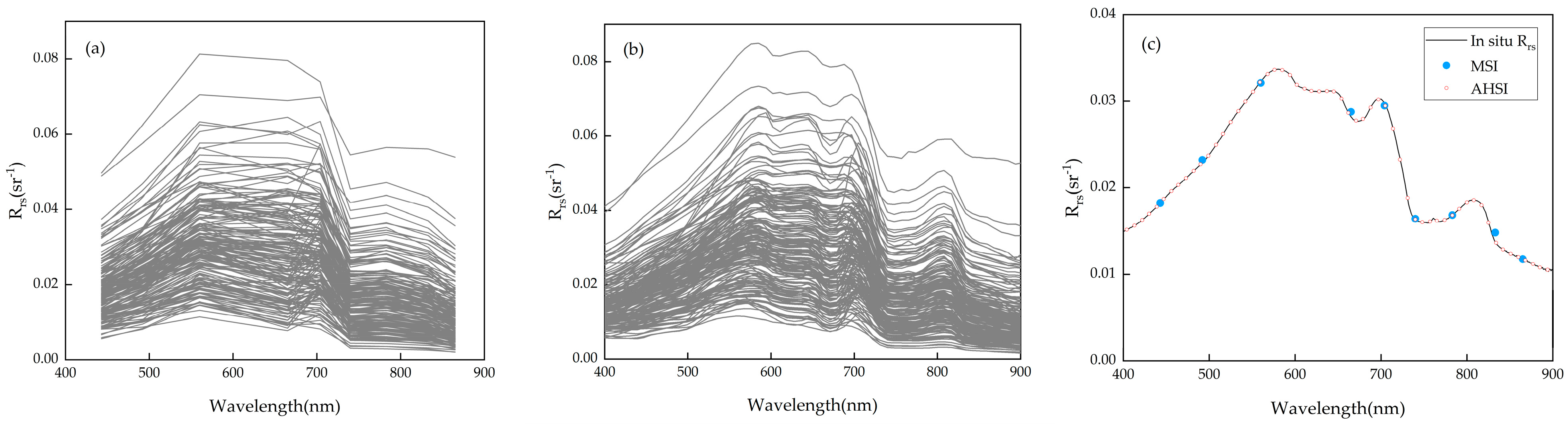
2.3.1. Satellite Band Simulation
2.3.2. Model Development
2.3.3. Satellite Data Preprocessing
2.3.4. Accuracy Assessment
3. Results
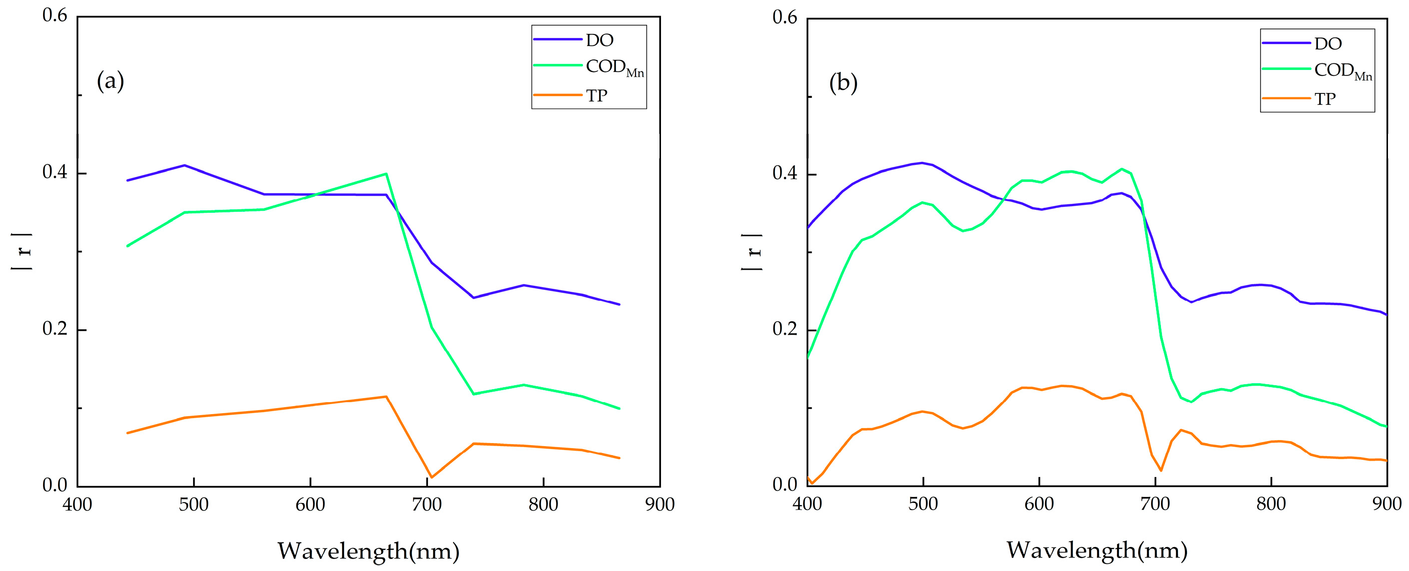
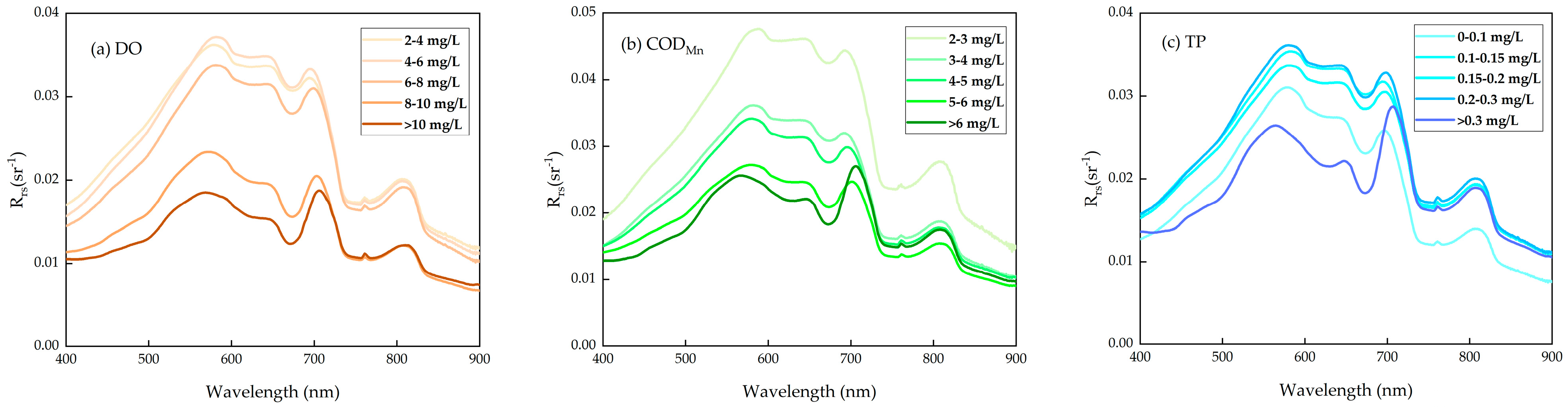
3.1. Spectral Response to Non-Optically Water Quality Parameter Variation
3.2. Development and Validation of Machine Learning Models
3.2.1. Model Structure and Inputs
3.2.2. Performances of Machine Learning Models
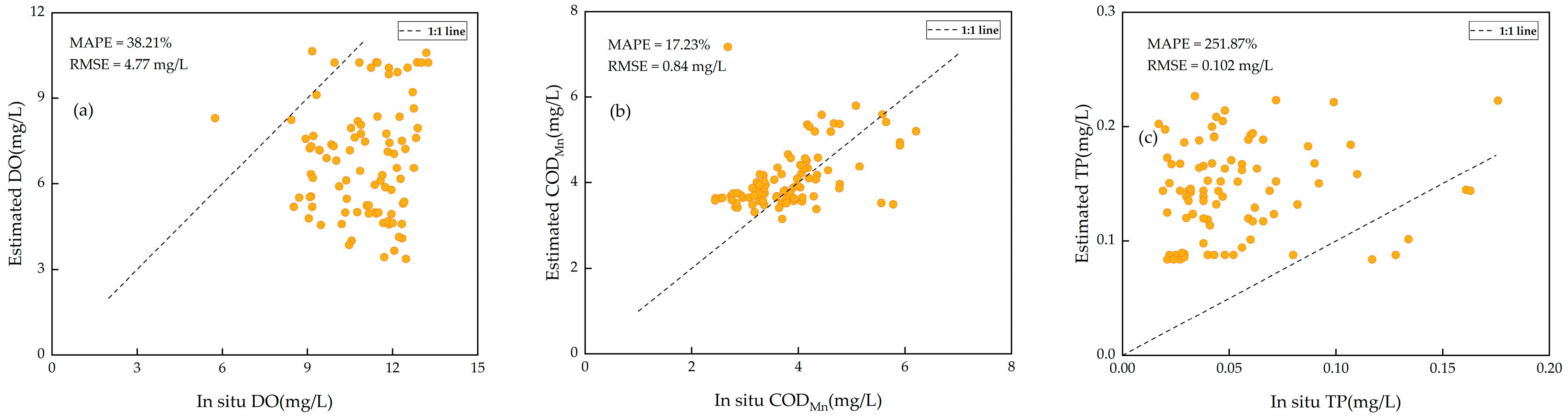
3.2.3. Further Validation on Taihu Lake
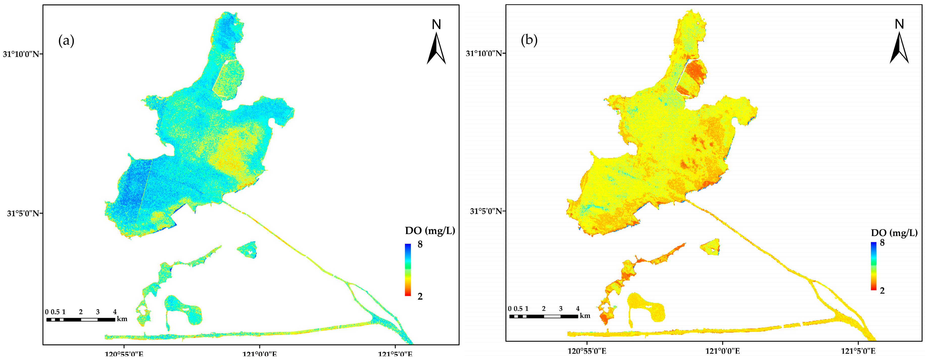
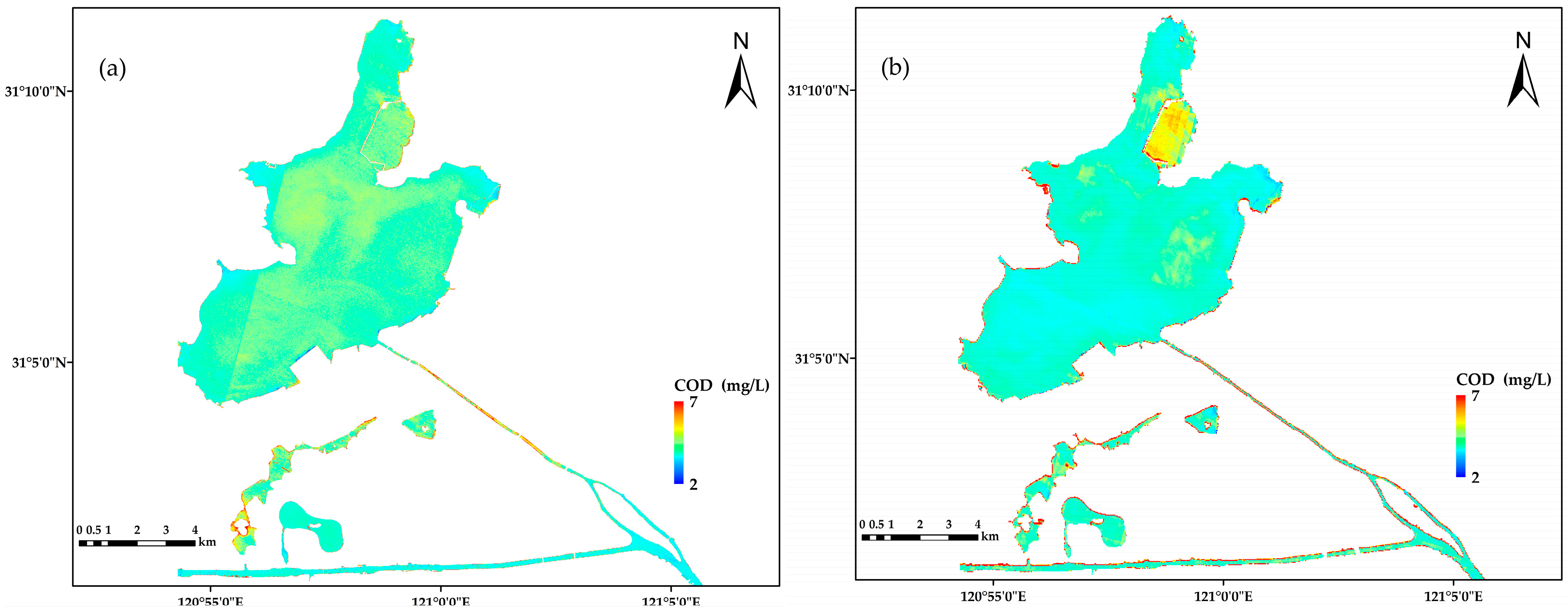
3.3. Water Quality Mapping
4. Discussion
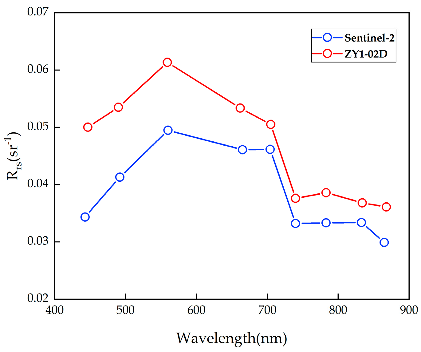
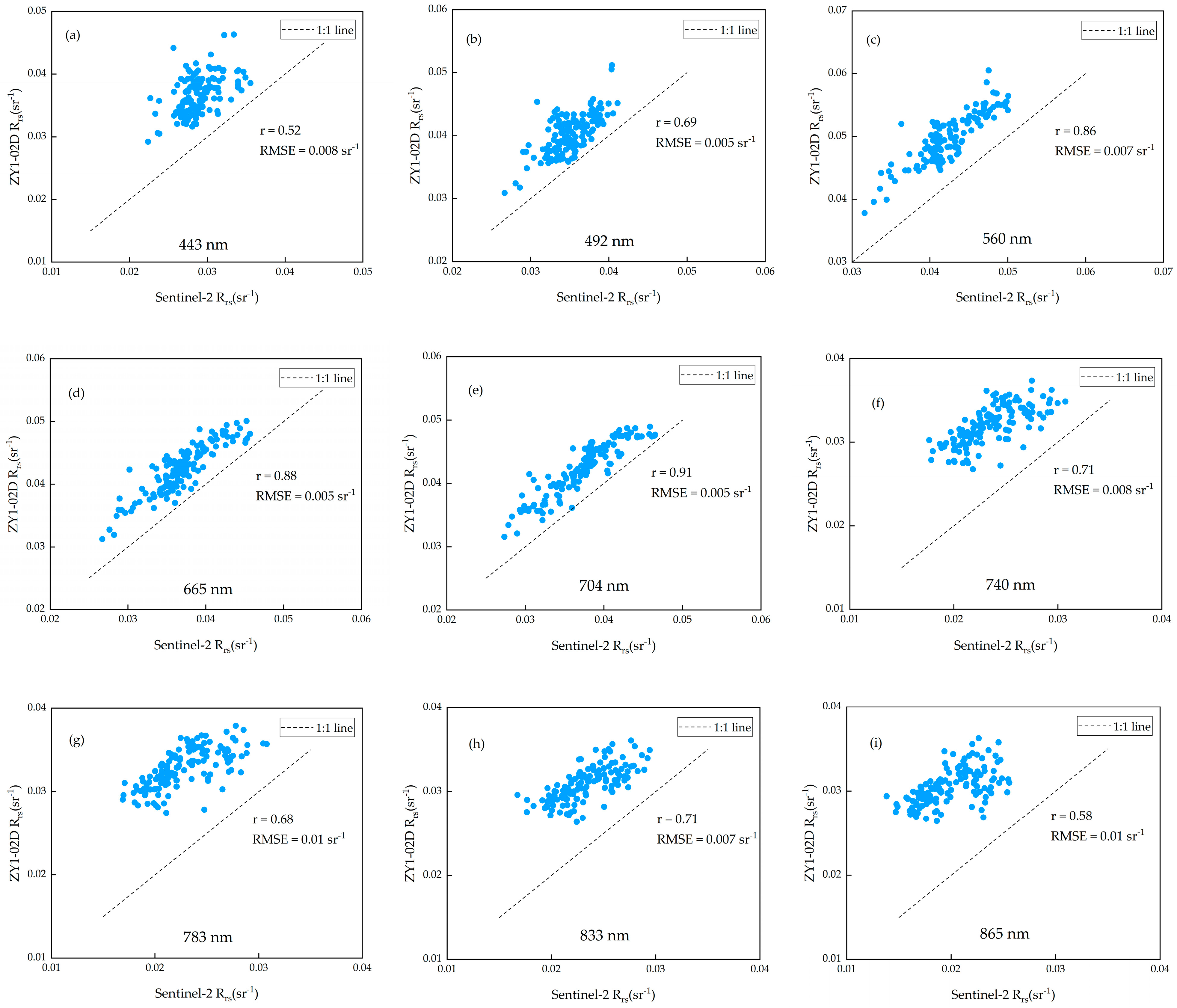
4.1. Comparison of Products between ZY1-02D and Sentinel-2
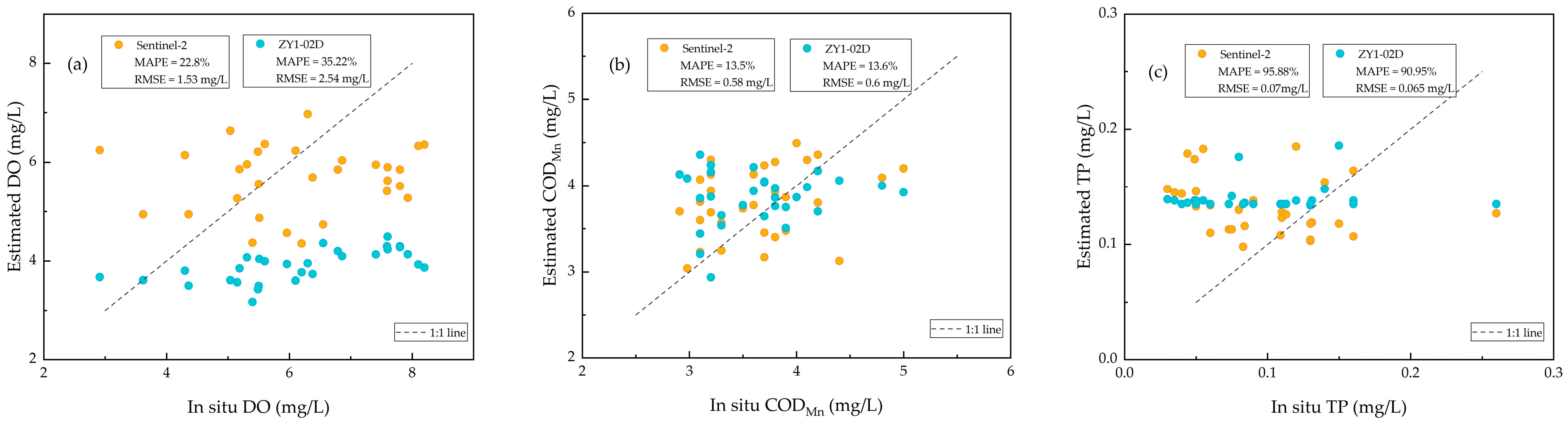
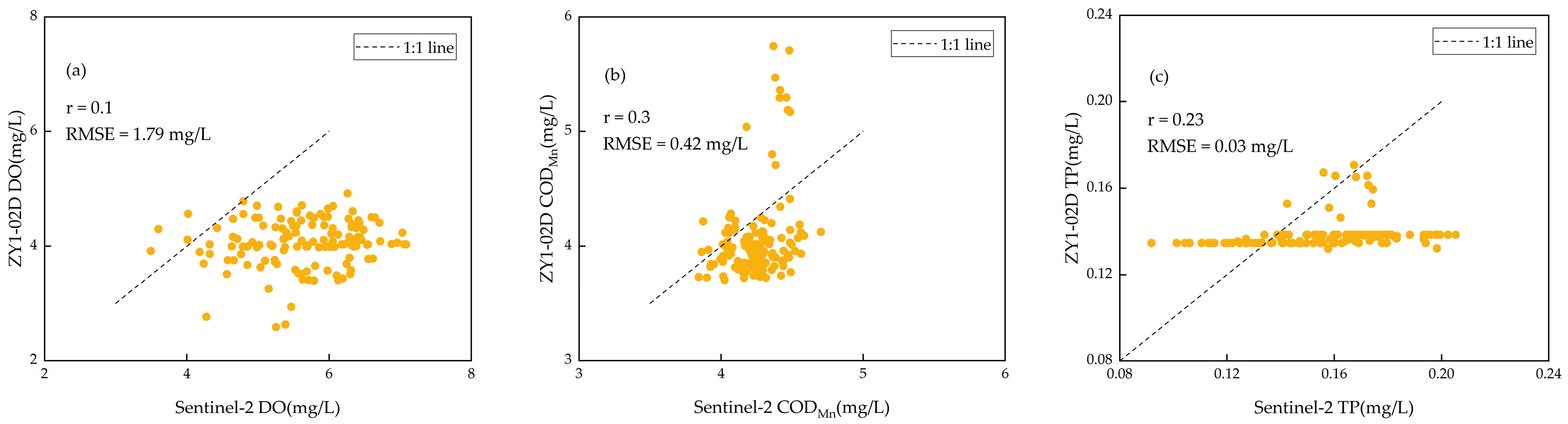
4.2. Comparison of Water Quality Products between ZY1-02D and Sentinel-2
4.3. Strengths and Limitations of the Models
5. Conclusions
Author Contributions
Funding
Data Availability Statement
Acknowledgments
Conflicts of Interest
References
- Miao, S.; Liu, C.; Qian, B.; Miao, Q. Remote sensing-based water quality assessment for urban rivers: A study in linyi devel-opment area. Environ. Sci. Pollut. Res. 2020, 27, 34586–34595. [Google Scholar] [CrossRef] [PubMed]
- Tham, T.T.; Hung, T.L.; Thuy, T.T.; Mai, V.T.; Trinh, L.T.; Hai, C.V.; Minh, T.B. Assessment of some water quality parameters in the Red River downstream, Vietnam by combining field monitoring and remote sensing method. Environ. Sci. Pollut. Res. 2022, 29, 41992–42004. [Google Scholar] [CrossRef]
- Chen, Y.; Fan, R.; Yang, X.; Wang, J.; Latif, A. Extraction of Urban Water Bodies from High-Resolution Remote-Sensing Imagery Using Deep Learning. Water 2018, 10, 585. [Google Scholar] [CrossRef]
- He, Y.; Jin, S.; Shang, W. Water quality variability and related factors along the yangtze river using landsat-8. Remote Sens. 2021, 13, 2241. [Google Scholar] [CrossRef]
- Vignolo, A.; Pochettino, A.; Cicerone, D. Water quality assessment using remote sensing techniques: Medrano Creek, Argentina. J. Environ. Manag. 2006, 81, 429–433. [Google Scholar] [CrossRef] [PubMed]
- Holyer, R.J. Toward universal multispectral suspended sediment algorithms. Remote Sens. Environ. 1978, 7, 323–338. [Google Scholar] [CrossRef]
- Sagan, V.; Peterson, K.T.; Maimaitijiang, M.; Sidike, P.; Sloan, J.; Greeling, B.A.; Maalouf, S.; Adams, C. Monitoring inland water quality using remote sensing: Potential and limitations of spectral indices, bio-optical simulations, machine learning, and cloud computing. Earth-Sci. Rev. 2020, 205, 103187. [Google Scholar] [CrossRef]
- Dey, J.; Vijay, R. A Critical and intensive review on assessment of water quality parameters through geospatial techniques. Environ. Sci. Pollut. Res. 2021, 28, 41612–41626. [Google Scholar] [CrossRef]
- Zhang, Y.; Wu, L.; Ren, H.; Liu, Y.; Zheng, Y.; Liu, Y.; Dong, J. Mapping Water Quality Parameters in Urban Rivers from Hyperspectral Images Using a New Self-Adapting Selection of Multiple Artificial Neural Networks. Remote Sens. 2020, 12, 336. [Google Scholar] [CrossRef]
- Qiao, Z.; Sun, S.; Jiang, Q.; Xiao, L.; Wang, Y.; Yan, H. Retrieval of Total Phosphorus Concentration in the Surface Water of Miyun Reservoir Based on Remote Sensing Data and Machine Learning Algorithms. Remote Sens. 2021, 13, 4662. [Google Scholar] [CrossRef]
- Guo, H.; Huang, J.J.; Chen, B.; Guo, X.; Singh, V.P. A Machine Learning-Based Strategy for Estimating Non-Optically Active Water Quality Parameters Using Sentinel-2 Imagery. Int. J. Remote Sens. 2020, 42, 1841–1866. [Google Scholar] [CrossRef]
- Li, Y.; Zhang, Y.; Shi, K.; Zhu, G.; Zhou, Y.; Zhang, Y.; Guo, Y. Monitoring spatiotemporal variations in nutrients in a largedrinking water reservoir and their relationships with hydrological and meteorological conditions based on Landsat 8 imagery. Sci. Total Environ. 2017, 599, 1705–1717. [Google Scholar] [CrossRef]
- Lim, J.; Choi, M. Assessment of water quality based on Landsat 8 operational land imager associated with human activities in Korea. Environ. Monit. Assess. 2015, 187, 1–17. [Google Scholar] [CrossRef]
- Gholizadeh, M.H.; Melesse, A.M.; Reddi, L. A comprehensive review on water quality parameters estimation using remote sensing techniques. Sensors 2016, 16, 1298. [Google Scholar] [CrossRef]
- Niroumand-Jadidi, M.; Bovolo, F.; Bruzzone, L. Novel Spectra-Derived Features for Empirical Retrieval of Water Quality Parameters: Demonstrations for OLI, MSI, and OLCI Sensors. IEEE Trans. Geosci. Remote Sens. 2019, 57, 10285–10300. [Google Scholar] [CrossRef]
- Al-Shaibah, B.; Liu, X.; Zhang, J.; Tong, Z.; Zhang, M.; El-Zeiny, A.; Faichia, C.; Hussain, M.; Tayyab, M. Modeling Water Quality Parameters Using Landsat Multispectral Images: A Case Study of Erlong Lake, Northeast China. Remote Sens. 2021, 13, 1603. [Google Scholar] [CrossRef]
- Huangfu, K.; Li, J.; Zhang, X.; Zhang, J.; Cui, H.; Sun, Q. Remote Estimation of Water Quality Parameters of Medium- and Small-Sized Inland Rivers Using Sentinel-2 Imagery. Water 2020, 12, 3124. [Google Scholar] [CrossRef]
- Gao, Y.; Gao, J.; Yin, H.; Liu, C.; Xia, T.; Wang, J.; Huang, Q. Remote sensing estimation of the total phosphorus concentration in a large lake using band combinations and regional multivariate statistical modeling techniques. J. Environ. Manag. 2015, 151, 33–43. [Google Scholar] [CrossRef]
- Chang, N.-B.; Xuan, Z.; Wimberly, B. Remote Sensing Spatiotemporal Assessment of Nitrogen Concentrations in Tampa Bay, Florida due to a Drought. Terr. Atmos. Ocean. Sci. 2011, 23, 467. [Google Scholar] [CrossRef]
- Mathew, M.M.; Rao, N.S.; Mandla, V.R. Development of regression equation to study the Total Nitrogen, Total Phosphorus and Suspended Sediment using remote sensing data in Gujarat and Maharashtra coast of India. J. Coast. Conserv. 2017, 21, 917–927. [Google Scholar] [CrossRef]
- Singh, A.; Jakubowski, A.R.; Chidister, I.; Townsend, P.A. A MODIS approach to predicting stream water quality in Wisconsin. Remote Sens. Environ. 2013, 128, 74–86. [Google Scholar] [CrossRef]
- Lu, S.; Deng, R.; Liang, Y.; Xiong, L.; Ai, X.; Qin, Y. Remote Sensing Retrieval of Total Phosphorus in the Pearl River Channels Based on the GF-1 Remote Sensing Data. Remote Sens. 2020, 12, 1420. [Google Scholar] [CrossRef]
- Liu, J.; Zhang, Y.; Yuan, D.; Song, X. Empirical Estimation of Total Nitrogen and Total Phosphorus Concentration of Urban Water Bodies in China Using High Resolution IKONOS Multispectral Imagery. Water 2015, 7, 6551–6573. [Google Scholar] [CrossRef]
- Dallosch, M.A.; Creed, I.F. Optimization of Landsat Chl-a Retrieval Algorithms in Freshwater Lakes through Classification of Optical Water Types. Remote Sens. 2021, 13, 4607. [Google Scholar] [CrossRef]
- O’Reilly, J.E.; Werdell, P.J. Chlorophyll algorithms for ocean color sensors—OC4, OC5 & OC6. Remote Sens. Environ. 2019, 229, 32–47. [Google Scholar] [CrossRef] [PubMed]
- Shanghai River (Lake) Report. 2021. Available online: http://swj.sh.gov.cn (accessed on 1 May 2022).
- Shanghai Seventh National Census Main Data Bulletin. Available online: http://tjj.sh.gov.cn/tjgb/20210517 (accessed on 1 May 2022).
- Yin, Z.-Y.; Walcott, S.; Kaplan, B.; Cao, J.; Lin, W.; Chen, M.; Liu, D.; Ning, Y. An analysis of the relationship between spatial patterns of water quality and urban development in Shanghai, China. Comput. Environ. Urban Syst. 2005, 29, 197–221. [Google Scholar] [CrossRef]
- Zhou, L.; Roberts, D.A.; Ma, W.; Zhang, H.; Tang, L. Estimation of higher chlorophylla concentrations using field spectral measurement and HJ-1A hyperspectral satellite data in Dianshan Lake, China. ISPRS J. Photogramm. Remote Sens. 2013, 88, 41–47. [Google Scholar] [CrossRef]
- Tang, J.; Guo, T.; Wang, X.; Wang, X.; Song, Q. The methods of water spectra measurement and analysis I: Above-water method. J. Remote Sens. 2004, 8, 37–44. [Google Scholar]
- Mobley, C.D. Estimation of the remote-sensing reflectance from above-surface measurements. Appl. Opt. 1999, 38, 7442–7455. [Google Scholar] [CrossRef]
- Zhong, Y.; Wang, X.; Wang, S.; Zhang, L. Advances in spaceborne hyperspectral remote sensing in China. Geo-Spat. Inf. Sci. 2021, 24, 95–120. [Google Scholar] [CrossRef]
- Zhu, P.; Liu, Y.; Li, J. Optimization and Evaluation of Widely-Used Total Suspended Matter Concentration Retrieval Methods for ZY1-02D’s AHSI Imagery. Remote Sens. 2022, 14, 684. [Google Scholar] [CrossRef]
- Cheng, Q.; Liu, B.; Li, T.; Zhu, L. Research on remote sensing retrieval of suspended sediment concentration in Hangzhou Bay by GF-1 satellite. Mar. Environ. Sci. 2015, 34, 558–563. [Google Scholar]
- Mountrakis, G.; Im, J.; Ogole, C. Support vector machines in remote sensing: A review. ISPRS J. Photogramm. Remote Sens. 2011, 66, 247–259. [Google Scholar] [CrossRef]
- Geladi, P.; Kowalski, B.R. Partial least-squares regression: A tutorial. Anal. Chim. Acta 1986, 185, 1–17. [Google Scholar] [CrossRef]
- McRoberts, R.E. Estimating forest attribute parameters for small areas using nearest neighbors techniques. For. Ecol. Manag. 2012, 272, 3–12. [Google Scholar] [CrossRef]
- Chen, T.; Guestrin, C. XGBoost: A Scalable Tree Boosting System. In Proceedings of the KDD’16: 22nd ACM SIGKDD Inter-national Conference on Knowledge Discovery and Data Mining, New York, NY, USA, 13–17 August 2016; pp. 785–794. [Google Scholar]
- Ma, Y.; Song, K.; Wen, Z.; Liu, G.; Shang, Y.; Lyu, L.; Du, J.; Yang, Q.; Li, S.; Tao, H.; et al. Remote Sensing of Turbidity for Lakes in Northeast China Using Sentinel-2 Images with Machine Learning Algorithms. IEEE J. Sel. Top. Appl. Earth Obs. Remote Sens. 2021, 14, 9132–9146. [Google Scholar] [CrossRef]
- Gao, Z.; Shen, Q.; Wang, X.; Peng, H.; Yao, Y.; Wang, M.; Wang, L.; Wang, R.; Shi, J.; Shi, D.; et al. Spatiotemporal Dis-tribution of Total Suspended Matter Concentration in Changdang Lake Based on In Situ Hyperspectral Data and Sentinel-2 Images. Remote Sens. 2021, 13, 4230. [Google Scholar] [CrossRef]
- Buma, W.; Lee, S.-I. Evaluation of Sentinel-2 and Landsat 8 Images for Estimating Chlorophyll-a Concentrations in Lake Chad, Africa. Remote Sens. 2020, 12, 2437. [Google Scholar] [CrossRef]
- Du, Y.; Zhang, Y.; Ling, F.; Wang, Q.; Li, W.; Li, X. Water Bodies’ Mapping from Sentinel-2 Imagery with Modified Normalized Difference Water Index at 10-m Spatial Resolution Produced by Sharpening the SWIR Band. Remote Sens. 2016, 8, 354. [Google Scholar] [CrossRef]
- Shenglei, W.; Junsheng, L.; Bing, Z.; Qian, S.; FangFang, Z.; Zhaoyi, L. A simple correction method for the MODIS surface reflectance product over typical inland waters in China. Int. J. Remote Sens. 2016, 37, 6076–6096. [Google Scholar] [CrossRef]
- Seegers, B.N.; Stumpf, R.P.; Schaeffer, B.; Loftin, K.A.; Werdell, P.J. Performance metrics for the assessment of satellite data products: An ocean color case study. Opt. Express 2018, 26, 7404–7422. [Google Scholar] [CrossRef] [PubMed]
- Cao, Z.; Ma, R.; Duan, H.; Pahlevan, N.; Melack, J.; Shen, M.; Xue, K. A machine learning approach to estimate chlorophyll-a from Landsat-8 measurements in inland lakes. Remote Sens. Environ. 2020, 248, 111974. [Google Scholar] [CrossRef]
- Shi, J.; Shen, Q.; Yao, Y.; Li, J.; Chen, F.; Wang, R.; Xu, W.; Gao, Z.; Wang, L.; Zhou, Y. Estimation of Chlorophyll-a Concen-trations in Small Water Bodies: Comparison of Fused Gaofen-6 and Sentinel-2 Sensors. Remote Sens. 2022, 14, 229. [Google Scholar] [CrossRef]
- Hafeez, S.; Wong, M.S.; Ho, H.C.; Nazeer, M.; Nichol, J.E.; Abbas, S.; Tang, D.; Lee, K.-H.; Pun, L. Comparison of Machine Learning Algorithms for Retrieval of Water Quality Indicators in Case-II Waters: A Case Study of Hong Kong. Remote. Sens. 2019, 11, 617. [Google Scholar] [CrossRef]
- Wang, X.; Gong, C.; Ji, T.; Hu, Y.; Li, L. Inland water quality parameters retrieval based on the VIP-SPCA by hyperspectral remote sensing. J. Appl. Remote Sens. 2021, 15, 042609. [Google Scholar] [CrossRef]
- Niroumand-Jadidi, M.; Bovolo, F.; Bruzzone, L.; Gege, P. Inter-Comparison of Methods for Chlorophyll-a Retrieval: Sentinel-2 Time-Series Analysis in Italian Lakes. Remote Sens. 2021, 13, 2381. [Google Scholar] [CrossRef]
- Warren, M.A.; Simis, S.G.H.V.; Vicente, M.; Poser, K.; Bresciani, M.; Alikas, K.; Spyrakos, E.; Giardino, C.; Ansper, A. Assessment of atmospheric correction algorithms for the Sentinel-2A MultiSpectral Imager over coastal and inland waters. Remote Sens. Environ. 2019, 225, 267–289. [Google Scholar] [CrossRef]
- Kuhn, C.; De Matos Valerio, A.; Ward, N.; Loken, L.; Sawakuchi, H.O.; Kampel, M.; Richey, J.; Stadler, P.; Crawford, J.; Striegl, R.; et al. Performance of Landsat-8 and Sentinel-2 surface reflectance products for river remote sensing retrievals of chlorophyll-a and turbidity. Remote Sens. Environ. 2019, 224, 104–118. [Google Scholar] [CrossRef]
- Xu, G.; Li, P.; Lu, K.; Tantai, Z.; Zhang, J.; Ren, Z.; Wang, X.; Yu, K.; Shi, P.; Cheng, Y. Seasonal changes in water quality and its main influencing factors in the Dan River basin. CATENA 2018, 173, 131–140. [Google Scholar] [CrossRef]


| No. | Date | The District of Shanghai | Number |
|---|---|---|---|
| 1 | 19 September 2018, 26 September 2018, 27 September 2018 | Jiading | 37 |
| 2 | 17 December 2018 | Jiading | 12 |
| 3 | 12 April 2019, 17 April 2019 | Qingpu | 21 |
| 4 | 21 May 2019, 22 May 2019 | Jiading | 11 |
| 5 | 7 April 2021, 8 April 2021 | Qingpu, Pudong | 25 |
| 6 | 9 May 2021, 10 May 2021 | Changning, Jinshan | 15 |
| 7 | 1 June 2021, 6 June 2021 | Qingpu, Chongming | 12 |
| 8 | 6 July 2021 | Chongming | 5 |
| 9 | 5 August 2021, 9 August 2021 | Xuhui, Yangpu | 17 |
| 10 | 7 September 2021 | Pudong | 8 |
| 11 | 12 October 2021 | Hongkou | 12 |
| 12 | 13 November 2021 | Yangpu | 8 |
| Total | / | / | 183 |
| Water Quality Parameters | Laboratory Measurement Methods | Mean | Min. | Max. | Std |
|---|---|---|---|---|---|
| DO | Iodometry method | 5.9 | 2.0 | 12.8 | 2.3 |
| CODMn | Permanganate index method | 4.58 | 2.10 | 11.40 | 1.58 |
| TP | Molybdenum antimony spectrophotometry | 0.172 | 0.041 | 0.664 | 0.093 |
| Sentinel-2A MSI | ZY1-02D AHSI | ||||
|---|---|---|---|---|---|
| Band Number | Wavelength (nm) | Resolution (m) | Band Number | Wavelength (nm) | Resolution (m) |
| 1 | 433–453 | 60 | 6–7 | 433–452 | 30 |
| 2 | 458–523 | 10 | 9–15 | 459–521 | 30 |
| 3 | 543–578 | 10 | 19–22 | 545–581 | 30 |
| 4 | 650–680 | 10 | 31–34 | 648–675 | 30 |
| 5 | 698–713 | 20 | 37 | 700–710 | 30 |
| 6 | 733–748 | 20 | 41–42 | 734–753 | 30 |
| 7 | 773–793 | 20 | 45–47 | 769–796 | 30 |
| 8 | 785–900 | 10 | 47–59 | 786–899 | 30 |
| 8A | 855–875 | 20 | 55–56 | 854–873 | 30 |
| Band Ratio | ||||
|---|---|---|---|---|
| DO | CODMn | TP | ||
| MSI | Rrs(B3)/Rrs(B4) | 0.4 * | 0.41 * | 0.12 |
| Rrs(B5)/Rrs(B4) | 0.38 * | 0.66 * | 0.42 * | |
| Rrs(B6)/Rrs(B4) | 0.25 * | 0.59 * | 0.43 * | |
| Rrs(B6)/Rrs(B7) | 0.32 * | 0.16 * | 0.02 | |
| Rrs(B7)/Rrs(B4) | 0.21 * | 0.56 * | 0.41 * | |
| AHSI | Rrs(B22)/Rrs(B33) | 0.44 * | 0.4 * | 0.06 |
| Rrs(B37)/Rrs(B31) | 0.35 * | 0.66 * | 0.44 * | |
| Rrs(B37)/Rrs(B33) | 0.4 * | 0.66 * | 0.4 * | |
| Rrs(B37)/Rrs(B34) | 0.4 * | 0.66 * | 0.41 * | |
| Rrs(B41)/Rrs(B33) | 0.29 * | 0.63 * | 0.43 * | |
| Rrs(B42)/Rrs(B45) | 0.34 * | 0.17 * | 0.03 | |
| Rrs(B45)/Rrs(B33) | 0.25 * | 0.6 * | 0.42 * | |
| Rrs(B47)/Rrs(B34) | 0.24 * | 0.6 * | 0.42 * | |
| Parameter | Variables | R2 | MAPE (%) | RMSE (mg/L) |
|---|---|---|---|---|
| DO | 5 | 0.21 | 29.98 | 2.18 |
| 9 | 0.32 | 29.30 | 2.02 | |
| 12 | 0.53 | 24.28 | 1.67 | |
| CODMn | 5 | 0.38 | 21.56 | 1.33 |
| 9 | 0.42 | 21.47 | 1.29 | |
| 12 | 0.65 | 17.99 | 1.0 | |
| TP | 5 | 0.08 | 37.69 | 0.096 |
| 9 | 0.27 | 39.88 | 0.086 | |
| 12 | 0.48 | 37.04 | 0.073 |
| Sentinel-2 | ZY1-02D | ||||||
|---|---|---|---|---|---|---|---|
| Parameter | Model | R2 | MAPE (%) | RMSE (mg/L) | R2 | MAPE (%) | RMSE (mg/L) |
| DO | SVR | 0.43 | 22.12 | 1.85 | 0.39 | 22.18 | 1.92 |
| PLSR | 0.34 | 28.24 | 1.98 | 0.35 | 27.19 | 1.97 | |
| KNN | 0.33 | 26.42 | 2.00 | 0.31 | 26.68 | 2.03 | |
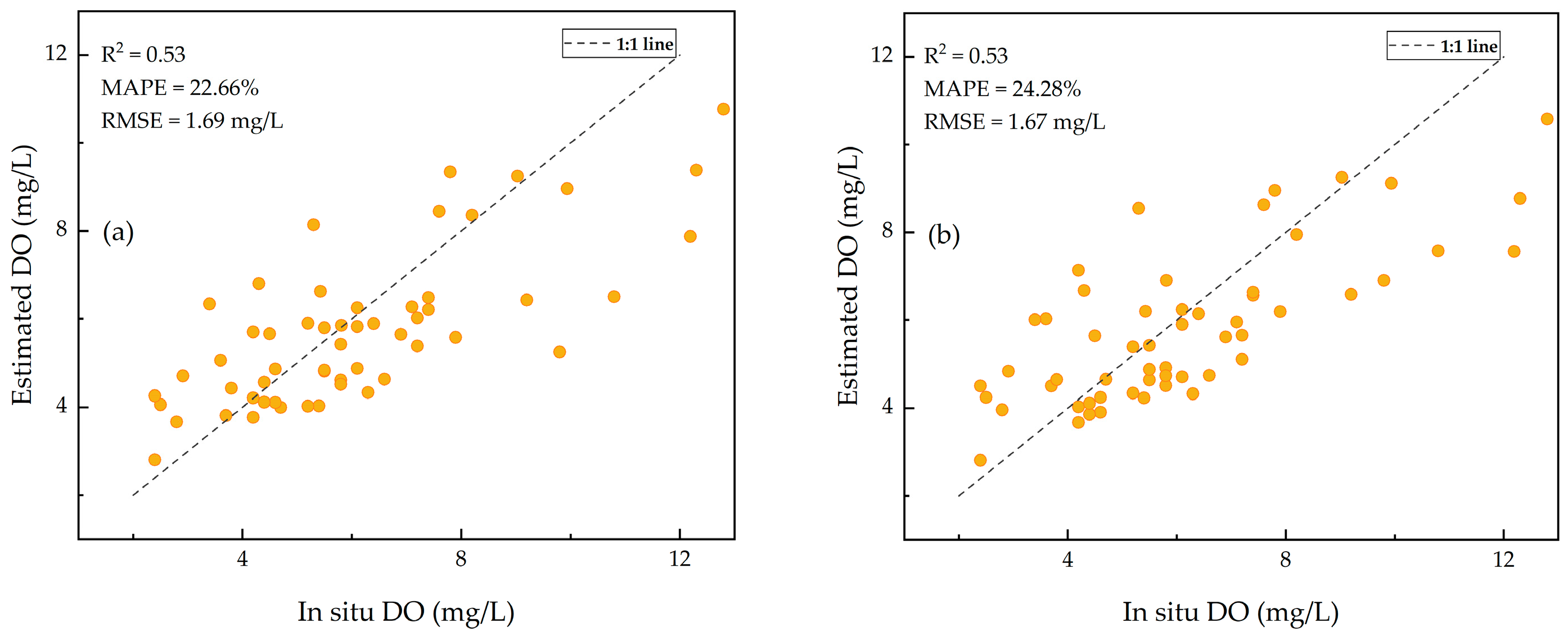
| XGBoost | 0.53 | 22.66 | 1.69 | 0.53 | 24.28 | 1.67 | |
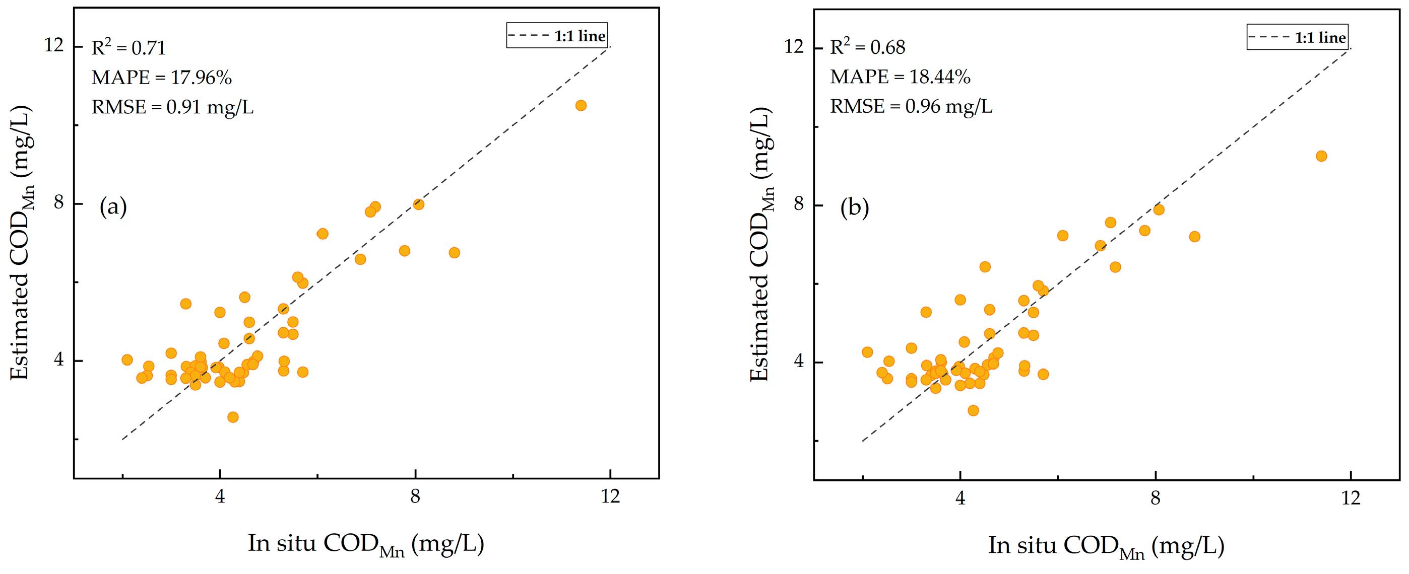
| CODMn | SVR | 0.71 | 17.96 | 0.91 | 0.68 | 18.44 | 0.96 |
| PLSR | 0.65 | 18.10 | 1.01 | 0.65 | 17.21 | 1.01 | |
| KNN | 0.65 | 17.11 | 1.00 | 0.66 | 17.03 | 0.99 | |
| XGBoost | 0.58 | 19.53 | 1.10 | 0.65 | 17.99 | 1.0 | |
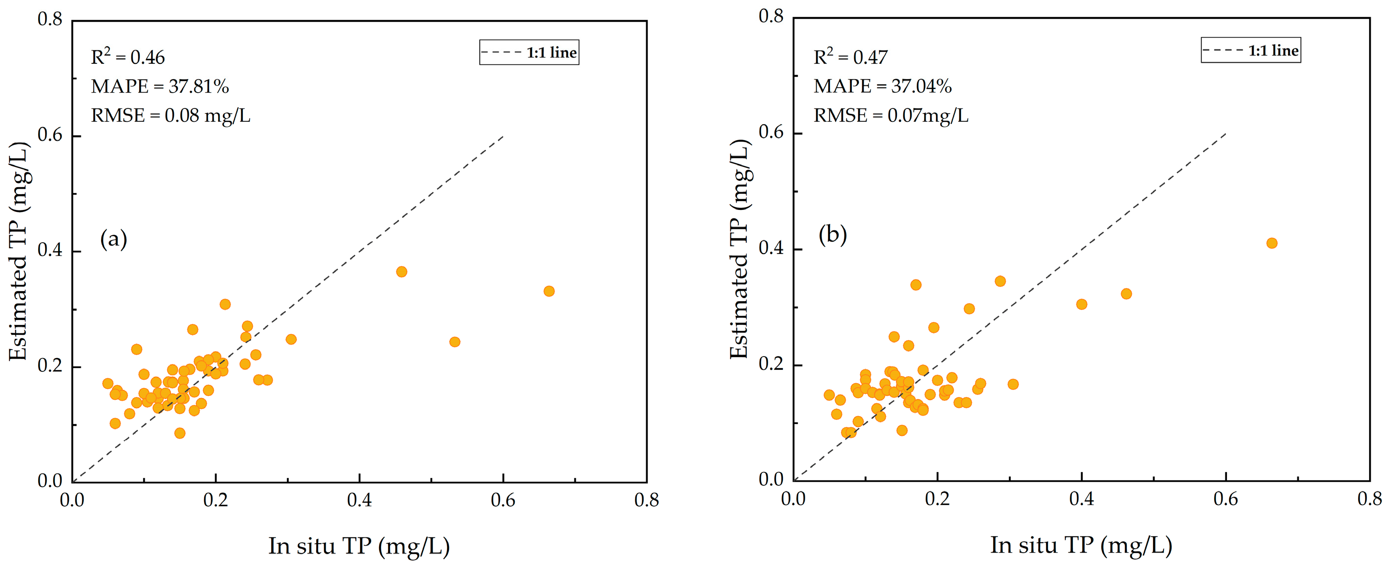
| TP | SVR | 0.46 | 37.81 | 0.08 | 0.36 | 46.97 | 0.086 |
| PLSR | 0.42 | 37.11 | 0.082 | 0.34 | 37.54 | 0.088 | |
| KNN | 0.43 | 37.18 | 0.082 | 0.46 | 37.67 | 0.079 | |
| XGBoost | 0.39 | 40.88 | 0.079 | 0.48 | 37.04 | 0.073 | |
Publisher’s Note: MDPI stays neutral with regard to jurisdictional claims in published maps and institutional affiliations. |
© 2022 by the authors. Licensee MDPI, Basel, Switzerland. This article is an open access article distributed under the terms and conditions of the Creative Commons Attribution (CC BY) license (https://creativecommons.org/licenses/by/4.0/).
Share and Cite
Yang, Z.; Gong, C.; Ji, T.; Hu, Y.; Li, L. Water Quality Retrieval from ZY1-02D Hyperspectral Imagery in Urban Water Bodies and Comparison with Sentinel-2. Remote Sens. 2022, 14, 5029. https://doi.org/10.3390/rs14195029
Yang Z, Gong C, Ji T, Hu Y, Li L. Water Quality Retrieval from ZY1-02D Hyperspectral Imagery in Urban Water Bodies and Comparison with Sentinel-2. Remote Sensing. 2022; 14(19):5029. https://doi.org/10.3390/rs14195029
Chicago/Turabian StyleYang, Zhe, Cailan Gong, Tiemei Ji, Yong Hu, and Lan Li. 2022. "Water Quality Retrieval from ZY1-02D Hyperspectral Imagery in Urban Water Bodies and Comparison with Sentinel-2" Remote Sensing 14, no. 19: 5029. https://doi.org/10.3390/rs14195029
APA StyleYang, Z., Gong, C., Ji, T., Hu, Y., & Li, L. (2022). Water Quality Retrieval from ZY1-02D Hyperspectral Imagery in Urban Water Bodies and Comparison with Sentinel-2. Remote Sensing, 14(19), 5029. https://doi.org/10.3390/rs14195029