Article

Coastal Waveform Retracking for HY-2B Altimeter Data by Determining the Effective Trailing Edge and the Low Noise Leading Edge

1
First Institute of Oceanography, Ministry of Natural Resources, Qingdao 266061, China
2
College of Oceanography and Space Informatics, China University of Petroleum, Qingdao 266058, China
3
National Satellite Ocean Application Service, Beijing 100081, China
4
Donghai Laboratory, Zhoushan 316021, China
*
Author to whom correspondence should be addressed.
Remote Sens. 2022, 14(19), 5026; https://doi.org/10.3390/rs14195026
Submission received: 30 July 2022 / Revised: 19 September 2022 / Accepted: 6 October 2022 / Published: 9 October 2022

Abstract

:
As an important remote sensing technology, satellite altimetry provides a large amount of observations of sea surface height over the global ocean. In coastal areas, the accuracy of satellite altimetry data decreases greatly due to issues arise in the vicinity of land, related to poorer geophysical corrections and artifacts in the altimeter reflected signals linked to the presence of land within the instrument footprint. To improve the application of HY-2B altimetry data in coastal areas, this study proposes a coastal waveform retracking strategy for HY-2B altimetry mission, which depends on the effective trailing edge and the leading edge, which are less affected by coastal ‘contamination’, to retrieve accurate waveform information. The HY-2B pass 323 and pass 196 data are reprocessed, and the accuracy of the reprocessing results in the range of 0–40 km offshore is validated against the tide gauge data and compared with the HY-2B standard SGDR data. According to the analysis conclusion, the accuracy of the reprocessed data is higher than that of the SGDR data and has good performance within 15 km offshore. For the pass 323, the mean value of correlation coefficient and RMS of the reprocessed data against the corresponding tide gauge data are 0.893 and 45.1 cm, respectively, in the range within 0–15 km offshore, and are 0.86 and 33.6 cm, respectively, in the range beyond 15 km offshore. For the pass 196, the mean value of correlation coefficient and RMS of the reprocessed data against the corresponding tide gauge data in the range within 0–12 km offshore are 0.84 and 33.0 cm, respectively, and in the range within 0–5 km offshore to the island are 0.90 and 29.3 cm, respectively, and in the range beyond 5 km offshore to the island are 0.92 and 36.2 cm, respectively, which are all better than the corresponding values of the SGDR data, especially in the range closed to the land. The results indicate that the proposed coastal waveform retracking strategy for HY-2B altimetry greatly improves the quality of HY-2B altimetry data in coastal areas.

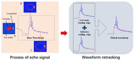
Graphical Abstract

1. Introduction

Satellite altimetry is designed to observe and record the variability of sea surface height and has developed into a mature remote sensing technology. Compared with traditional measurements, it rapidly and globally measures on a large spatial scale with high precision and can serve marine science and global climate change research. The basic principle of satellite altimetry is to send a pulse signal vertically toward the sea surface and then record the double-traveling time of the pulse signal reflected from the sea surface, which forms an echo whose shape is known as the ’waveform’. Meanwhile, the on-board tracker (as an a priori device that determines the analysis window of the altimeter to prevent the altimeter losing the surface track) measures the standard range containing the bias of several centimeters between the altimeter and the satellite nadir point, which is mainly caused by the Raleigh noise in the pulse signals.
To correct the deviation of standard range measurement provided by the on-board retracker, a necessary process called ’waveform retracking’ is applied to provide the tracking range correction, significant wave height, and backscatter coefficient correction. The principle of waveform retracking is inversing the sea surface information from the waveform data based on the waveform model. Depended on microwave scattering theory, scholars have described the waveform using the Brown theoretical ocean model (referred to as the Brown model), which was proposed by Brown and refined by Hayne [1,2]. The Brown model expounds the ideal relationship between the pulse signal traveling time and the pulse energy reflected from the sea surface: an increasing leading edge and a decreasing trailing edge with a certain amount of thermal noise, as shown in Figure 1. In Figure 1, the midpoint of the leading edge, which is known as the ’mid-power point’, is used to estimate the distance between the satellite altimeter and the sea surface. The increasing time of leading edge is mainly dependent on the significant wave height (SWH) at the nadir, with a longer increasing time associated with a larger SWH. The amplitude of the echo can be converted into a measurement of the backscatter coefficient σ0 on the basis of the instrument calibration. The slope of the trailing edge depends on the antenna mispointing angle, which is approximately 0.3°. The precision of waveform retracking largely depends on the quality of altimetry waveform data, usually, the waveform data observed on the open ocean is the best, which is reflected by the pure-water surface and contains stable noise information.
According to different areas, waveform retracking can be divided into waveform retracking for polar, open ocean, and coastal areas. The earliest waveform retracking was applied to altimetry data in polar regions and the main problem is that the pulse signal reflected from the ice surface is totally different to the ocean pulse signal. Since, many algorithms are based on statistical properties of the waveform at that time, such as the β-parameter algorithm, OCOG, the threshold algorithm and the improved threshold algorithm [3,4,5,6]. While, waveform retracking for the open ocean always considers the noise of waveform data and adopts maximum likelihood parameter estimation (MLE) with the Brown model, which is the standard processing for altimetry mission and usually improved by reducing the correlative bias between the fitted parameters of the waveform model [7,8].
The coastal areas, as the main activity area for humans, are under pressure because of climate change, population growth, expanding economic development, and meeting the risks from storm surge events and sea level rise. Altimetry data provides an irreplaceable contribution to pollutant dispersal, coastal erosion, flood risk assessment, extreme weather forecasting, etc. In recent years, researchers have paid much attention to coastal areas and have accumulated more accurate satellite altimetry data in the range within 0–40 km offshore using new waveform retracking strategies.
The main problem of coastal waveform retracking is not only the noise of data but also the ‘pollution’ of the waveform data, which means the standard waveform retracking process of altimetry products may lead an extra range bias and have to handle the distorted part of the waveform before fitting. For the coastal waveform, the leading edge of the waveform is usually totally fitted without any modification, and the trailing edge of the waveform is always partially fitted to avoid misinformation. In addition, under the condition of a certain performance of the waveform retracking algorithm, various types of coastal waveforms can be processed reasonably based on waveform classification.
Waveform retracking based on subwaveform is an important method for coastal waveform retracking that adopts a complete leading edge and a small trailing edge to effectively fit the distorted waveform. The representative subwaveform retracking strategies are adaptive leading edge subwaveform retracking (ALES) and spatial-temporal altimeter retracking (STAR). ALES takes the adaptive subwaveform as the ‘optimal’ choice to yield suboptimal estimates when the coastal waveform is polluted. The adaptive subwaveform window is determined through the linear relationship between the tracking point and the SWH [9]. The coastal altimetry data of the Jason-1, Jason-2, and Envisat missions were reprocessed successfully using the ALES algorithm in the X-TRACK/ALES satellite data operational framework, and new coastal satellite altimetry data products and thematic datasets have been distributed [10,11,12]. However, the ALES algorithm fails when the ‘pollution’ is close to the leading edge of the waveform [13]. According to the spatial-temporal information of continuous waveforms integrated using random conditions, STAR separates subwaveforms from a single waveform by sparse representation. Then, the Dijkstra algorithm is used to obtain a reliable estimation from the polluted waveform [14]. The STAR algorithm shows superiority in dealing with extremely noisy waveforms, but the reliability of the derived sea surface height (SSH) data is reduced due to data smoothing and the reduction in SSH variability information in coastal areas [15]. Additionally, the subwaveform is adaptively determined by the size of the homogeneous surface, such as sea surface slick [16].
Compared with subwaveform retracking, total-waveform fitting is steadier and needs to carefully address the distortion of the waveform trailing edge. For the coastal ‘contamination’, strong reflections on the coastal sea surface leave a hyperbolic trajectory through waveform space, and there is a geometric relationship between the reflections and sample gates of the waveform [17,18], which gives the physical possibility to position the distorted part of coastal waveform. Simply comparing along-track echograms from different satellite data of the same spatial-temporal area, some objects called ‘bright targets’ on the sea surface can be estimated using geometric analysis [19]. Furthermore, according to the relative location of coastal ‘pollution’ in relation to the satellite nadir, the corresponding waveform noise is removed from the along-track echograms, and along-track waveforms with clean trailing edges are obtained [20]. When the distortions of the waveform are irregular and fragmentary, the waveform distortion parts can be detected directly by the shape characteristic. Multiple Brown-peak (MBP) waveform retracking uses adaptive peak detection (APD) to recognize the peak noise of the Brown-peak waveform and processes the distorted trailing edge of a single waveform efficiently [21,22].
Furthermore, the shape classification of coastal waveform can improve the efficiency of waveform retracking algorithms, which is the initial step for coastal waveform retracking process systems [23,24,25]. The advantage of waveform classification is that it solves the problem of a single waveform retracking strategy being unable to process all coastal waveforms with the same precision. Based on the a priori knowledge of different waveform retracking algorithms, coastal waveforms are divided appropriately into several types and can be processed to maximally improve the quality of the data. However, it is necessary to comprehensively consider the fitting-deviation between different waveform retracking strategies [21,26].
In short, the quality of coastal altimetry data has been greatly improved. Accurate observation extends to a range of approximately 5 km offshore thanks to the development of coastal waveform retracking. For most coastal waveform retracking strategies, the judgment of a coastal waveform is a credible leading edge and a terrible trailing edge. The influence of coastal ‘pollution’ on the leading edge of the waveform is ignored, and the effective trailing edge information is not considered adequately, which contributes to recovering accurate coastal altimetry observations.
The HY-2A satellite equipped with a radar altimeter, as the first Chinese marine dynamic environmental satellite, was launched in 2011. Subsequently, HY-2B, HY-2C and HY-2D were successfully launched in 2018, 2020, and 2021, respectively, forming a marine dynamic environment-monitoring satellite constellation. Currently, HY-2B, HY-2C, and HY-2D are in orbit, providing high-quality observation data for ocean scientific research and monitoring. The accuracy of HY-2B satellite coastal altimetry data is always lower than that in the open ocean due to the inapplicability of the MLE4 retracker in coastal areas, limiting the application of the HY-2B data product in the coastal area. In this study, a coastal waveform retracking strategy for HY-2B satellite altimetry is proposed. By intercepting the leading edge of the waveform with less noise and confirming the effective part of the trailing edge, accurate estimations of coastal waveforms can be recovered. In addition, the coastal waveform retracking strategy proposed in this study prevents waveform classification and the boundary dividing for open ocean and coastal areas and has good performance both in open and coastal sea areas. The data accuracy and reliability of HY-2B altimeter data within the range of approximately 0–15 km offshore are greatly improved. The study areas and the HY-2B altimetry data used are introduced in Section 2. Section 3 introduces the waveform models and the coastal waveform retracking strategy proposed in this study. The waveform retracking results of the coastal HY-2B altimetry data are presented in Section 4. The validation and discussion are showed in Section 5. The main conclusions are given in Section 6.

2. Study Areas and Data

The HY-2B satellite is equipped with a traditional dual-frequency (Ku-band and C-band) altimeter. The repetition cycle of the HY-2B altimeter is 14 days, and 386 passes cover the global ocean. The 20Hz Ku-band echo waveform data included in the standard Sensor Geophysical Data Records (SGDR) provided by the National Satellite Ocean Application Service (NSOAS) are used in this study for waveform retracking. In addition, the SGDR data also contain the original result of the waveform retracking by the MLE4 retracker and the range corrections from different sources [27]. The tide gauge data to validate the accuracy of the retracking results of the HY-2B altimetry waveform are the Permanent Service for Mean Seal Level (PSMSL) data from the University of Hawaii Sea Level Center and include the raw tide information.
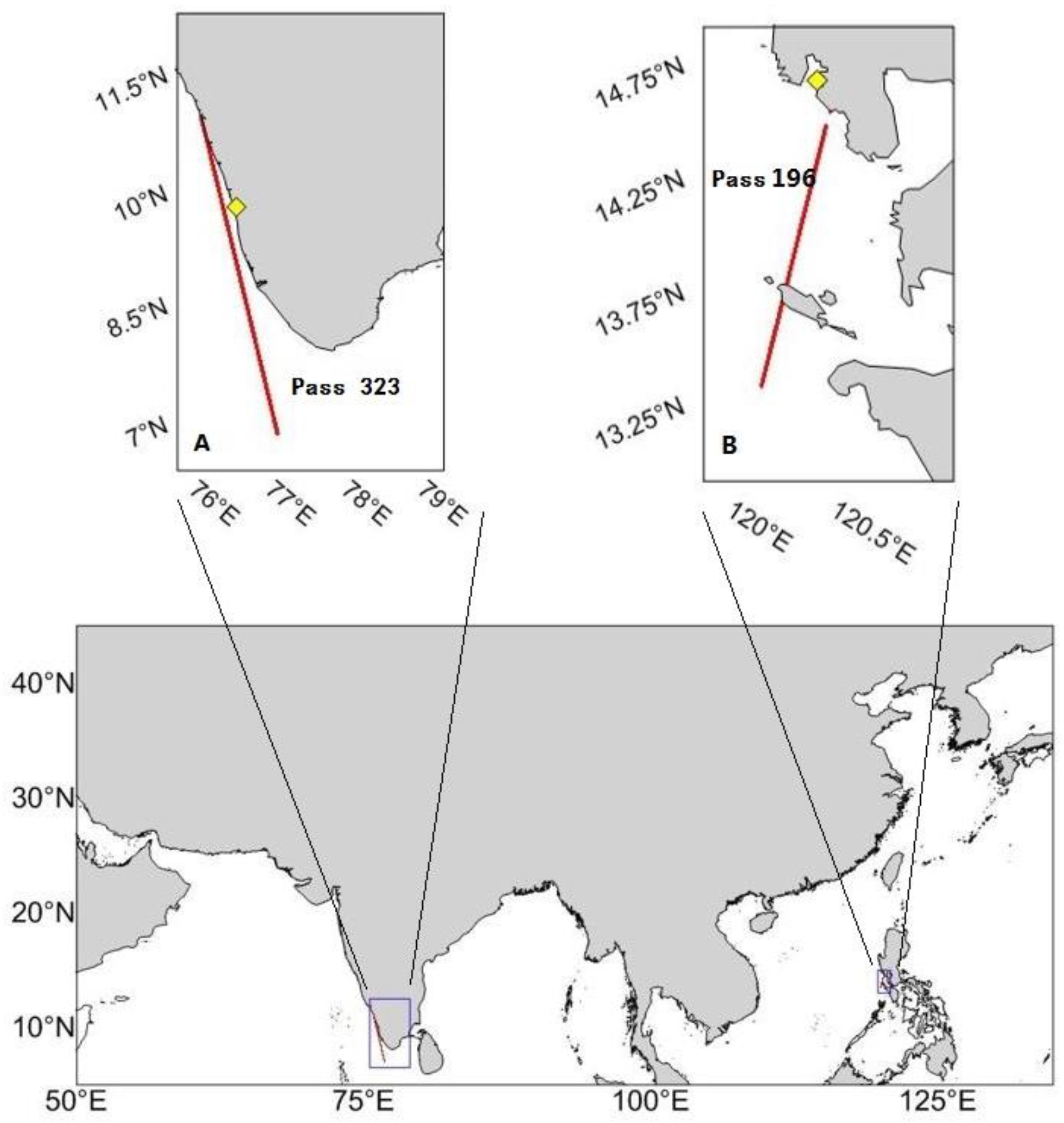
According to the available of tide gauge measurement data and the HY-2B altimeter orbit data, two areas are selected as study areas: the 0–40 km offshore area in the southwest of the Indian Peninsula (area A) and the 0–40 km offshore area in the southwest of the Philippine Islands (area B), as shown in Figure 2.
Area A is shown in the upper left corner of Figure 2. The pass 323 data of the HY-2B altimeter are selected in this study. Pass 323 is an ascending orbit, and its ground trajectory is parallel to the shoreline, so it has the largest proportion of data affected by coastal land in theory. The corresponding tide gauge station at Cochin (PSMSL Station ID 174, 9.967°N, 76.267°E) is located in this area. According to the time match of the tide gauge data and the HY-2B altimetry data, 15 cycles of altimetry data from 16 February 2019, to 9 November 2019, are used in this study (partial cycles are excluded due to the absence of satellite altimetry data or the lack of tide observations).
Area B is shown in the upper right corner of Figure 2. To verify the influence when the observation mode of HY-2B altimeter transforms from ocean to land and from land to ocean, the pass 196 data of the HY-2B altimeter are selected in this study. Pass 196 is a descending orbit, and the geographical conditions on both sides of the orbit are more complicated. In the range of 13.75°N to 14°N, the satellite flies over coastal islands, completing observation mode transition. The corresponding tide gauge station at Subic Bay (PSMSL Station ID 382, 14.765°N, 120.252°E) is located in this area. According to the time match of the tide gauge data and the satellite altimetry data, 38 cycles of altimeter data from 28 January 2019, to 10 August 2020, are used in this study.

3. Method

3.1. The Retracking Functional Form

To accurately fit the waveform, two variants of the Brown model are selected as the basis for waveform retracking: the Brown model with the second-order Bessel function [28] and the Brown model based on the roughness of the sea surface [29].
The Brown model with the second-order Bessel function fits the ocean-like waveforms in this study. Compared with the first-order Bessel function Brown model, this model can more accurately fit the waveforms with a larger mispointing angle. The specific description of this model is as follows:
W ( t ) = a ξ P u [ 1 + e r f ( u 1 ) ] exp ( v 1 ) a ξ P u 2 [ 1 + e r f ( u 2 ) ] exp ( v 2 ) + T n
where
a ξ = exp ( 4 sin 2 ξ γ ) γ = sin 2 ( θ 0 ) 1 2 ln ( 2 ) e r f ( x ) = 2 x 0 x e t 2 d t u 1 = t τ a 1 σ c 2 2 σ c v 1 = α 1 ( t τ a 1 σ c 2 2 ) α 1 = δ β 2 8 u 2 = t τ a 2 σ c 2 2 σ c v 1 = α 2 ( t τ a 2 σ c 2 2 ) α 2 = δ δ = 4 c γ h cos ( 2 ξ ) β = 4 γ ( c h ) 1 / 2 sin ( 2 ξ ) h = H ( 1 + H / R e ) σ c 2 = σ s 2 + σ p 2 σ s = S W H 2 c
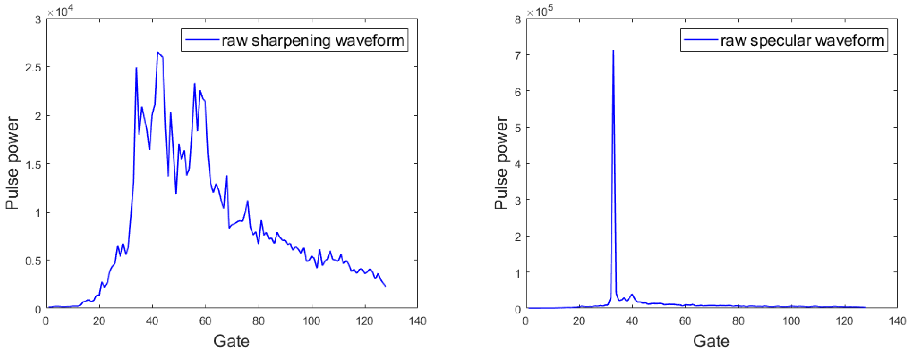
Considering the existence of specular waveforms and waveforms with a small trailing edge slope (the sharpening waveform shown in Figure 3), which are caused by a calm sea surface, the Brown model based on sea surface roughness is applied. The specific description of this model is as follows:
W s ( t ) = a ξ P u 2 [ 1 + e r f ( u ) ] exp ( v )
where
u = t τ α σ c 2 2 σ c v = a ( t τ α σ c 2 2 ) α = 4 c Γ h Γ = 4 γ m s s 4 m s s + γ
the parameters of the two models are same, where aξ is calculated using the mispointing angle ξ. The value of γ depends on the antenna beam width θ0. Pu is the amplitude of the waveform. t is the echo traveling time. τ is the midpoint of the leading edge. c is the speed of light. h is the corrected height calculated from the satellite orbit height H and the Earth curvature Re. σc is the composite backscattering coefficient. σp is the corresponding width of the radar point target, and the HY-2B altimeter uses 0.513tr, where tr is the continuous power gate interval time equal to 3.125 ns. Γ is a parameter defined by γ and the mean square slope (mss) of the reflected surface and is used to determine the slope of the waveform trailing edge. When the mss value is close to infinity, the Brown model based on sea surface roughness is transformed into the first-order Bessel function Brown model. For the Brown model with a second-order Bessel function, the main fitting parameters are τ, SWH, Pu, and ξ (referred to as the WLS4), while the fitted parameters of the Brown model based on sea surface roughness are τ, SWH, Pu, and Γ(referred to as the MB4). The iterative method of the model adopts weight least squares fitting based on the Nelder–Mead algorithm [30].

3.2. Waveform Retracking Method

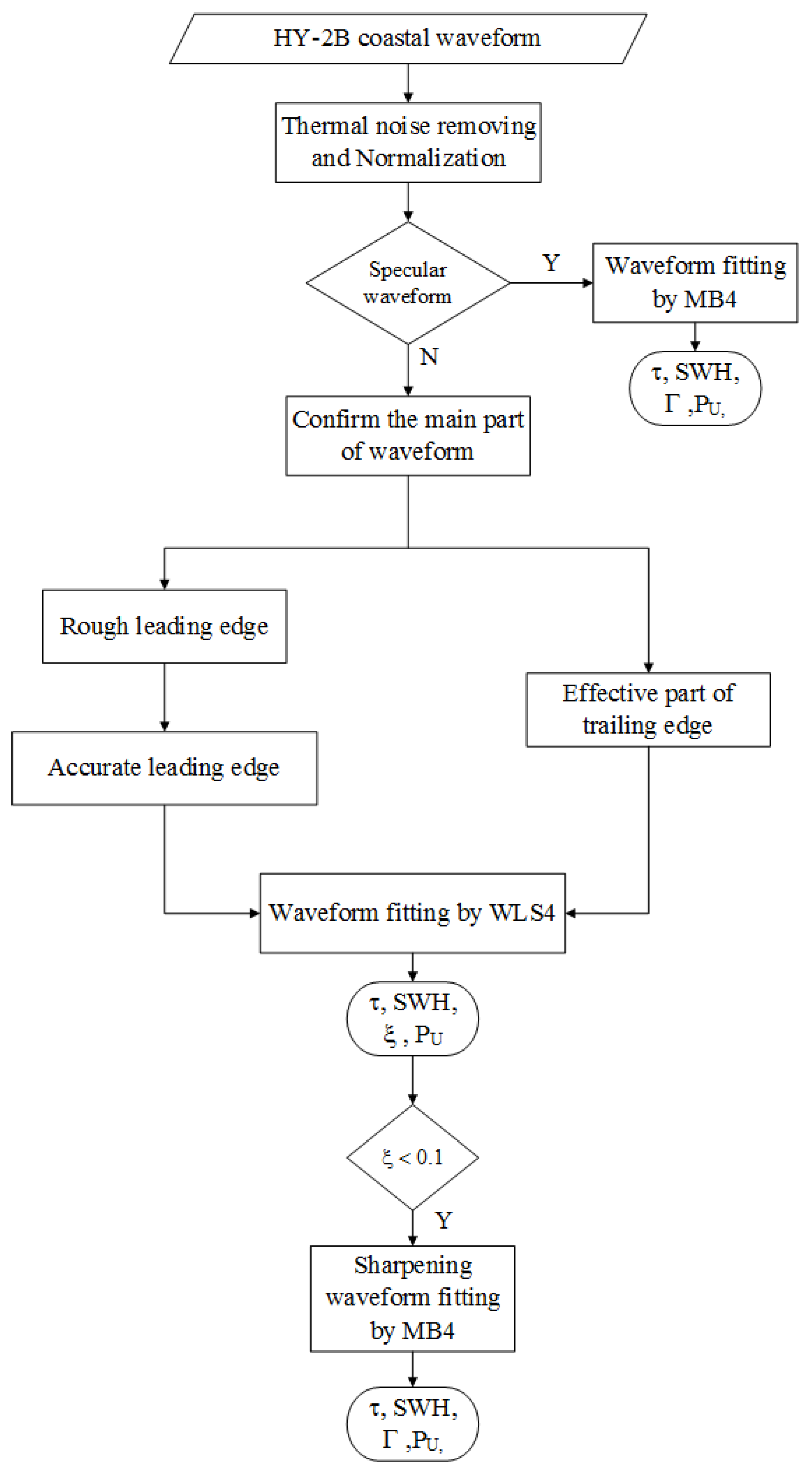
To improve the data accuracy and enhance the data application of HY-2B satellite altimeter in coastal areas, this study designs a coastal waveform retracking strategy to process the HY-2B altimetry coastal waveform data. The strategy picks the effective part of the leading edge and trailing edge of coastal waveforms out then retrieves the accurate parameters of the observed sea surface based on the classic waveform models. The details are shown in Figure 4. The main processing of this method includes thermal noise removal and power normalization, specular echo processing and non-specular echo processing. The specular echo waveform is fitted by the MB4. The crucial steps of non-specular echo processing are as follows: first, confirming the rough leading edge part of the waveform and then obtaining the accurate leading edge according to the reference gates; second, identifying the steady trailing edge part of the waveform by searching the effective trailing edge; finally, weighting and fitting the processed leading edge and trailing edge of the waveform by the WLS4 to derive the parameters of the sea surface and according to the mispointing angle to recognize and refit the sharpening waveform by the MB4.

3.2.1. Thermal Noise Removal and Normalization

A simple average-value filter in the 1–25th gates is applied firstly to eliminate the extremely abnormal noise. Based on the statistic of HY-2B altimeter coastal waveforms, the gates from 5 to 10 are chosen to calculate the thermal noise and remove it from the echo signal. The maximum of the eight-point moving average at each gate is taken as the normalization factor, which is subsequently adjusted according to the accurate leading edge power to ensure that the maximum of the leading edge is approximately 0.9 normalized power. The power mentioned subsequently refers to the normalized power in this study.

3.2.2. Specular Echo Processing

When the measurement footprint of altimeter covers a calm sea surface, the waveform is similar to a ‘single peak’ (as shown in the left of Figure 3), which is called specular echo and needs to be handled separately. In the HY-2B satellite altimetry data processing framework, the OCOG algorithm is used to address specular echoes. In this study, because the number of specular echoes is small in the study area, we screen them out if the pulse peakness (PP) is larger than 5 and the average power of the waveform tail is smaller than 0.25. Then, we take the major peak as the main part of specular echo to fit by the MB4. The PP index is calculated as follows [31]:
P P = 31.5 × p max i = 5 64 p i
where, the Pi is the power of ith gate.

3.2.3. Non-Specular Echo Processing

Non-specular waveforms are the main processing objects in this study, the leading edge and the trailing edge of the non-specular waveforms are disposed of in different ways. For the leading edge, a rough leading edge is identified by the ’normal ending gate’ and the ’possible ending gate’ of the leading edge. Then, the reference ending power of the leading edge is provided from the reference gates to obtain an accurate leading edge that contains less noise. For the trailing edge of the waveform, a steady attenuation part of the trailing edge is searched for as the effective trailing edge, and the tail of the trailing edge is taken as the supplement. The results are obtained by fitting the processed leading edge and effective trailing edge with the WLS4 and then picking the sharpening waveforms out by the mispointing angle to refit by the MB4.
  • Confirming the main part of waveform
Coastal waveforms sometimes have several continuous noise gates around the beginning of the leading edge, which is avoided by confirming the main part of the waveform in this study. All gates with power exceeding a threshold are screened out, and then the widest part is taken as the main part of the waveform and searched backward to find the starting gate. The first gate with increasing power serves as the starting gate of the main part of the waveform. The threshold is an empirical value taken as 0.35 in this study.
It is necessary to determine the main part of the waveform. When the satellite nadir approaches the coast, the general leading edge forward search method has a false detection of the leading edge or contains noise information in the leading edge. If the beginning and the end of the leading edge are both affected by coastal ’pollution’, SWH retrieval will be extremely inaccurate.
  • Leading edge processing
Generally, the ideal leading edge has the following characteristics: the power of the leading edge increases from fast to slow, and the growth rate is largest at the midpoint of the leading edge; the power growth rate is zero at the end of the leading edge, and then the power of the echo starts decreasing. Therefore, the top-power gate of the waveform is often thought to be the ending gate of the leading edge. The detection of the leading edge in this study includes rough leading edge detection and accurate leading edge detection. For rough leading edge detection, the first power-decreasing gate after the beginning of the waveform main part is taken as the ‘normal ending gate of the leading edge (NEG)‘ if the power of the NEG is higher than the next gate by more than 0.12; otherwise, the search for the NEG continues forward.
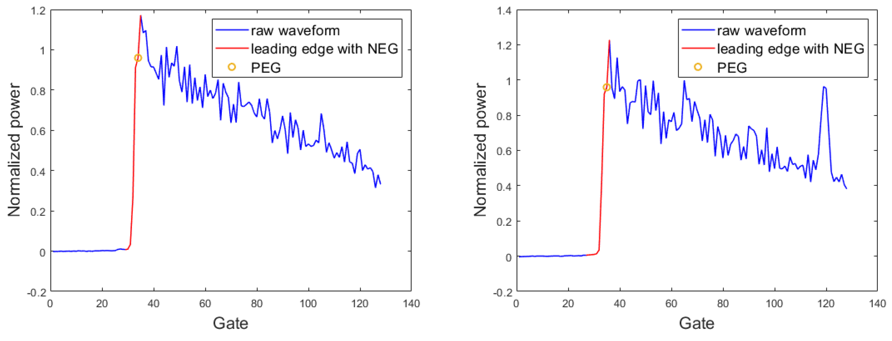
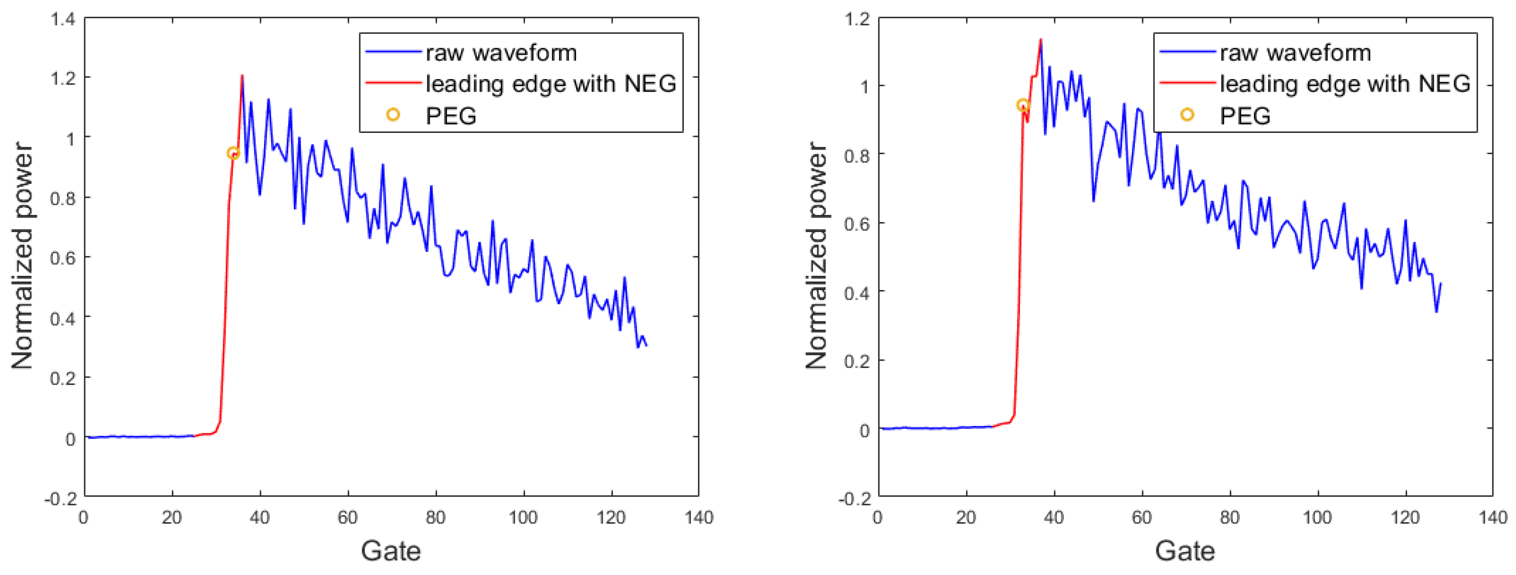
In addition, two special types of gates before the NEG are taken as the ‘possible ending gate of the leading edge (PEG)‘ for the rough leading edge. The first type of PEG is a gate with high power, but the increasing power suddenly slows down, as shown in Figure 5. The second type of PEG is a gate with a power slightly larger than that of the next gate, as shown in Figure 6. Both kinds of PEG indicate the coastal influence on the leading edge and are meaningful to the detection of the leading edge. The absolute power difference between the PEG and the next gate is less than 0.08, and there is only one NEG and no more than one PEG for a single waveform.
The ending gate of the rough leading edge is selected between the NEG and the PEG. If there is no PEG, the NEG is chosen. Otherwise, the PEG is chosen under the reliability judgment. The judgment criteria are that the power of the PEG is higher than that of most gates on the trailing edge and that the decay rate of the trailing edge varies significantly. Both PEGs marked in Figure 7 do not meet the criteria and cannot be taken as the ending gate of the rough leading edge.
Due to coastal influence, the rough leading edge includes extra noise gates. In this study, two reference gates provide the reference ending power of the leading edge to remove noisy gates from the rough leading edge. The selection of two reference gates is introduced as follows, and a rough leading edge with fewer than three gates is not processed.
The first reference gate is the first gate with increasing power after the ending of the rough leading edge. The second reference gate is decided based on the first reference gate. Both reference gates need to check whether there is a gate whose power is lower than the reference gate over 0.1 in its next five gates. Otherwise, the reference gate is replaced to avoid the reference gate being located at a wide distortion of the waveform. The second reference gate is the first gate after the first reference gate whose power meets the following relationship:
P sec o n d P f i r s t ( i f i r s t ) × 0.0065
where, the i is the ith gate after the first reference gate (i = first + 1,first + 2.80). 0.0065 is an empirical value, which is related with the theoretical waveform trailing edge with 0.3° mispointing angle.
Before deriving the reference ending power of the accurate leading edge, the reliability of reference gates is analyzed by the parameter C, which is defined as follows:
C = P f i r s t P sec ( sec f i r s t ) × 0.008
where 0.008 is the decay rate of theoretical waveform trailing edge with 0.3° mispointing angle.
The range from −0.1 to 0.1 is selected as the confident interval for C. C = 0 means that the second reference gate is not found within a certain search range. C > 0.1 means that the first reference gate is affected and unreliable. C < −0.1 indicates that the second reference gate is affected and unreliable. The value of C only reflects the relative reliability of two reference gates.
According to the more reliable reference gate and the power decay rate of approximately 0.008, the reference ending power of the leading edge is calculated using the power of the reference gate plus the power equal to the gate distance between the reference gate and the rough leading edge ending gate multiplied by 0.008. Based on the reference ending power of the leading edge, an accurate leading edge is obtained after removing the noise gates.
The removed gates correspond to the edge of the circular measurement footprint, which is affected by coastal ‘contamination’ [32]. Furthermore, the following types of rough leading edges are not processed by this step: (1) there are no PEGs, and C falls in the confident interval; (2) there are no gates with power close to the reference power of the leading edge ending; and (3) the trend of the trailing edge is increasing or the trend of attenuation is not obvious.
  • The processing of trailing edge
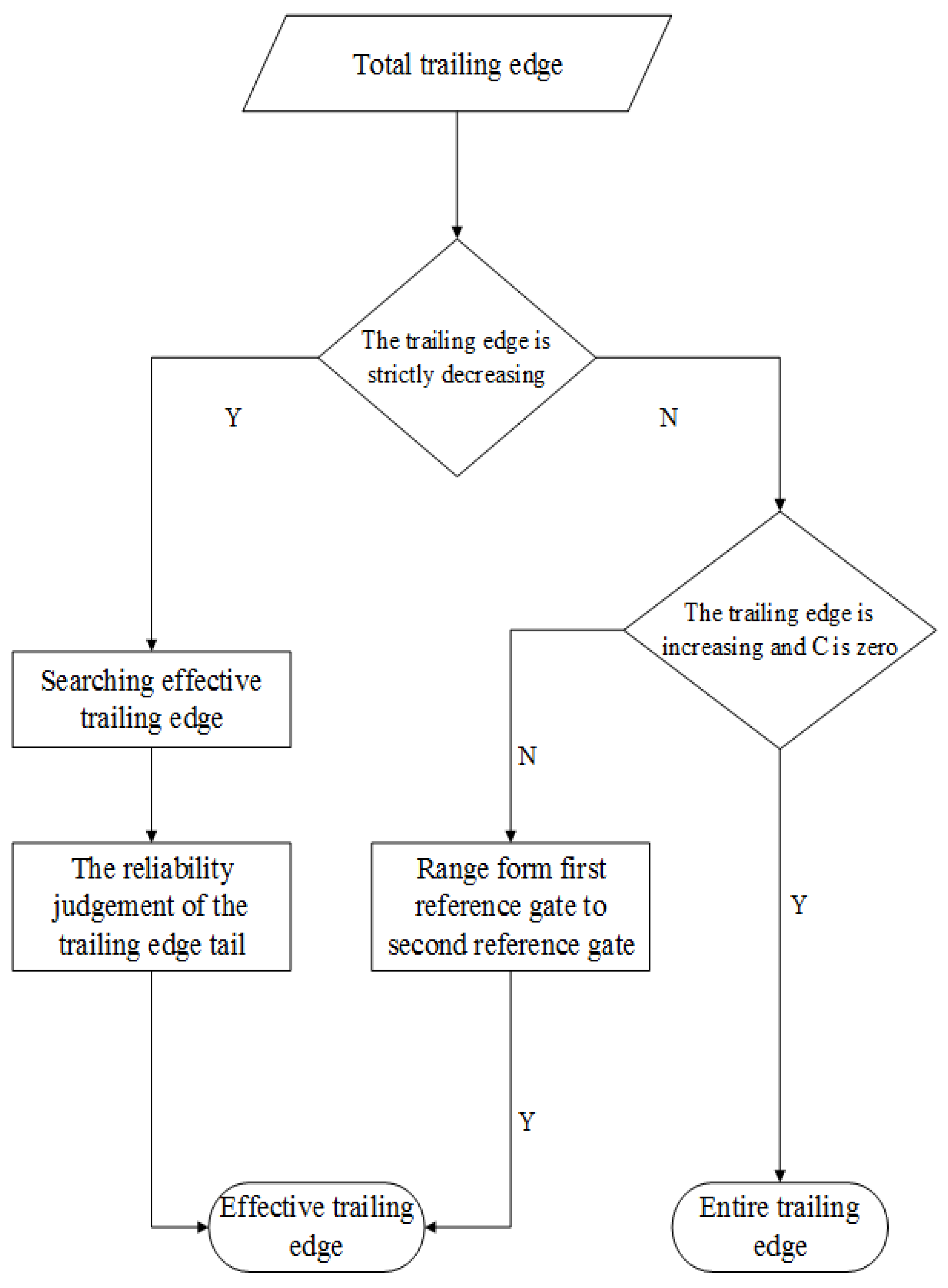
Usually, coastal ‘contamination’ initially appears in the annulus measurement footprint, and the circular measurement footprint survives. However, when the satellite nadir is close to the shoreline, the annulus measurement footprint covers more pure sea surface, while the circular measurement footprint entirely covers the coastal ‘pollution’, which means that the distortion of the waveform is located around the leading edge. More steady and effective information on the trailing edge is retained within a certain range offshore. Therefore, an effective trailing edge search method is proposed. The effective part of the trailing edge is identified by the power slope between each gate and the fixed gate to reduce the influence of waveform distortion on waveform retracking. For determining the width of distorted waveform, Peng [21] gives some suggestions to avoid influencing the precision of fitting, however, to retrieve the coastal data as possible, this article takes a more radical way and the choice of effective trailing edge reaching parameters are empirical values based on the statistics of real HY-2B altimeter waveform. The details of the effective trailing edge are shown in Figure 8.
First, we confirm the power-changing trend of the entire trailing edge through linear fitting.
If the power-changing trend of the entire trailing edge is essentially rising and the parameter C is zero, or the second reference gate is close to the lowest power gate of the trailing edge, the trailing edge is processed as follows: if the trend of the trailing edge is rising, the total trailing edge is not processed and weighted as the accurate leading edge; if the second reference gate is close to the lowest power gate of the trailing edge, the range of the effective trailing edge is from the first reference gate to the second reference gate.
Except as previously discussed, the trailing edge is processed as follows:
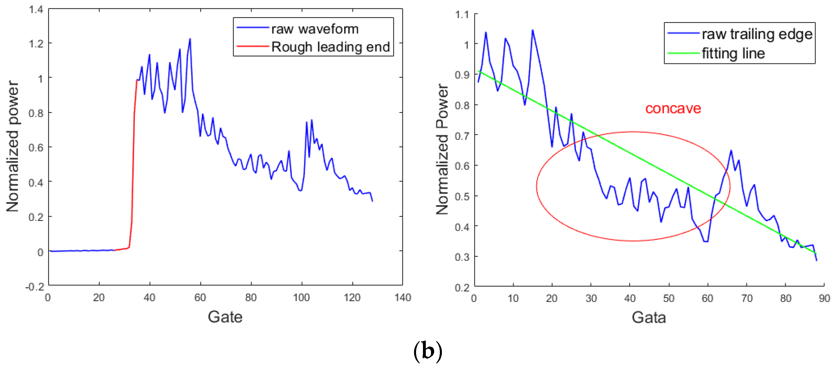
Depending on the linear-fitting power, the distortions of more than 15 gates with a power higher than the value of the linear-fitting power are removed from the range of the effective trailing edge. The distorted trailing edge will deviate from the fitting line to form a ‘convex‘ or ‘concave‘, as shown in Figure 9. According to the number of distortions, there are ‘convex‘ (Figure 9a) or ‘concaves‘ (Figure 9b).
Based on the above processing, the lowest power gate of the trailing edge is used as the fixed gate to calculate the power slope at each gate of the trailing edge. According to the gate distance threshold, the trailing edge containing the nine gates with the largest power slope is divided into several parts. The widest part is the effective trailing edge. When the power difference between the lowest power gate and some trailing edge gates is smaller than 0.0025, the headmost is selected as the fixed gate to ensure that the searching range of effective trailing edge is the absolutely decreasing trend. The gate distance threshold is 12.
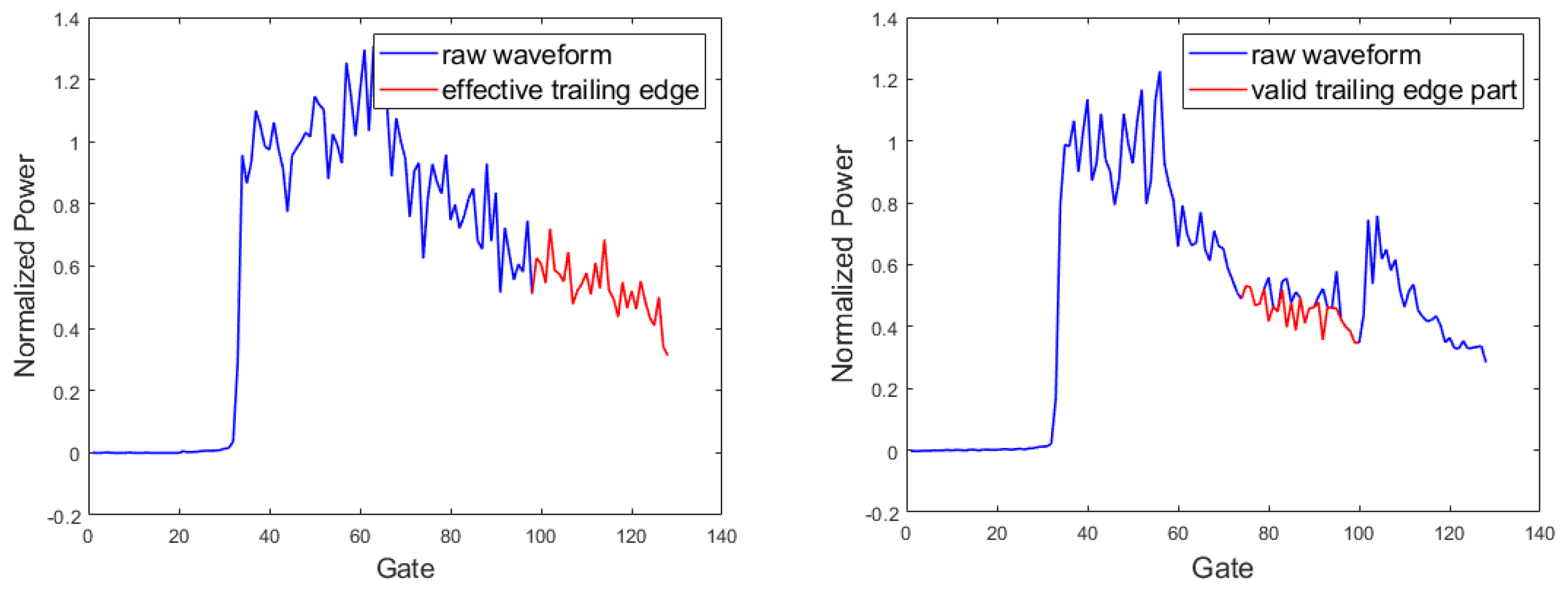
Then, the effective trailing edge is linearly fit and the power of linear power adding a 0.5 times trailing edge oscillation is taken to modify the noise gates. The noise gates are those with a power beyond linear power adding a 1.5 times trailing edge oscillation, and the trailing edge oscillation is the average of the absolute power difference between the top and the bottom of each peak that the effective trailing edge consists of. The modified effective trailing edge is shown in Figure 10.
Once the range of the effective trailing edge does not include the range of the 100th–128th gates, the availability of the trailing edge tail is checked. If the ten-gate average values of the 100th–128th gates are decreasing in order and the least, the 100th–128th gates are taken as the supplement for the effective trailing edge.
  • Weighting and fitting
Weighting the gates depends on the process of the leading edge and trailing edge. Since an accurate a priori value of the mispointing angle is unavailable for the distorted coastal waveform, four-parameter fitting is adopted based on the WLS (WLS4). The initial values of the normalized echo amplitude and mispointing angle are 1 and 0.3°, respectively, and the initial SWH is provided from SGDR data.
The sharpening waveform is detected by the mispointing angle of the WLS4-fitting and refitted by the MB4 to derive more accurate estimations. The sharpening waveform has a mispointing angle smaller than 0.1° according to the fitting result of the WLS4.

4. Waveform Retracking Results

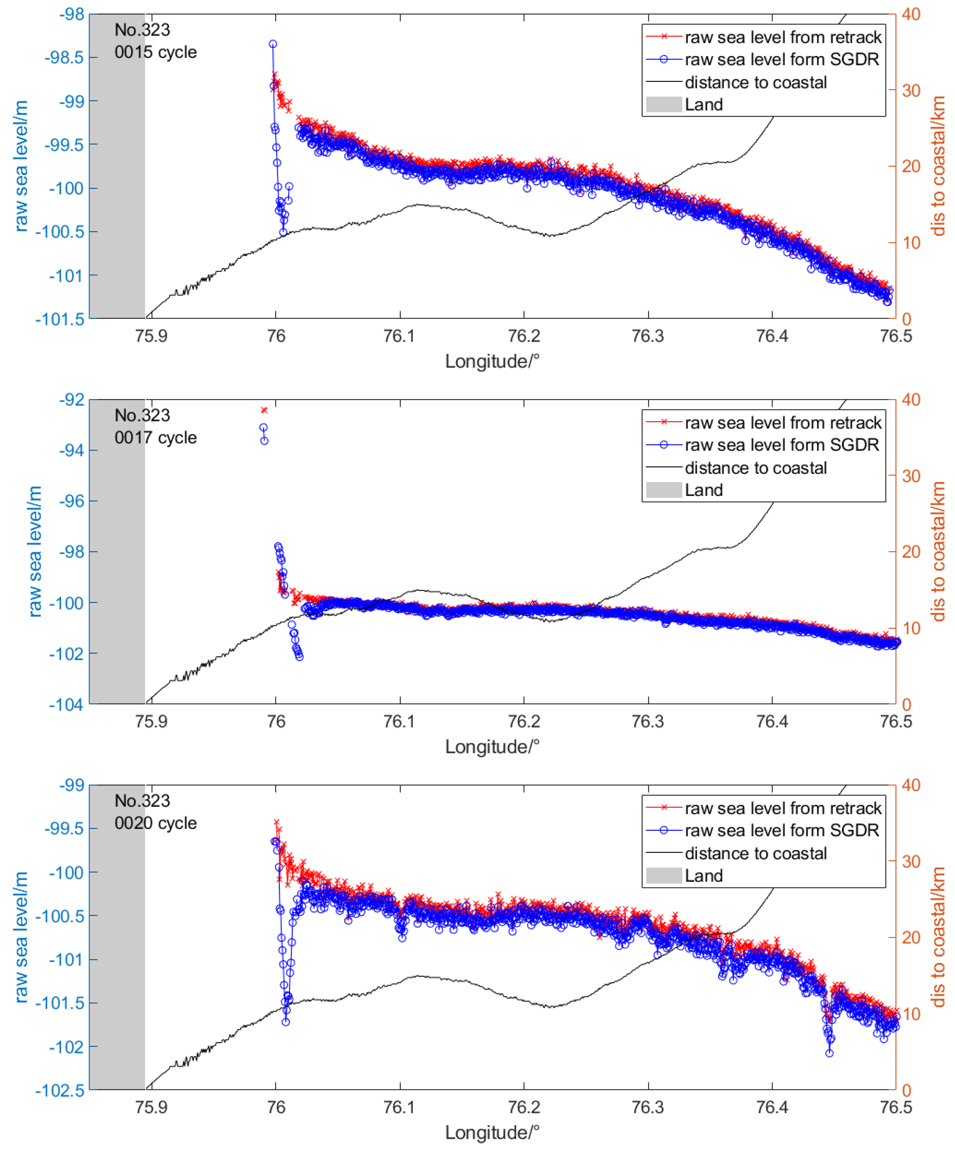
Depending on the waveform retracking strategy described in Section 3, 20hz waveform data of the HY-2B pass 323 and pass 196 have been reprocessed. In this section, we show the along-track raw sea level (RSL) of the reprocessed data and the HY-2B SGDR data. Additionally, some waveform retracking results are illustrated in Figure 11.
The RSL, sea surface height without any range corrections except the instrumental correction, is used to qualitatively analyze the reprocessing results of waveform retracking by comparing with the HY-2B standard SGDR data, and its calculation formula is as follows:
r a w   s e a   l e v e l = a l t i t u d e r e t r a c k e d   r a n g e
where
r e t r a c k e d   r a n g e r e t r a c k i n g = t r a c k i n g   r a n g e + r e t r a c k i n g   r a n g e   c o r r e c t i o n + i n s t r u m e n t a l   c o r r e c t i o n s
r e t r a c k e d   r a n g e S G D R = r e t r a c k i n g   r a n g e
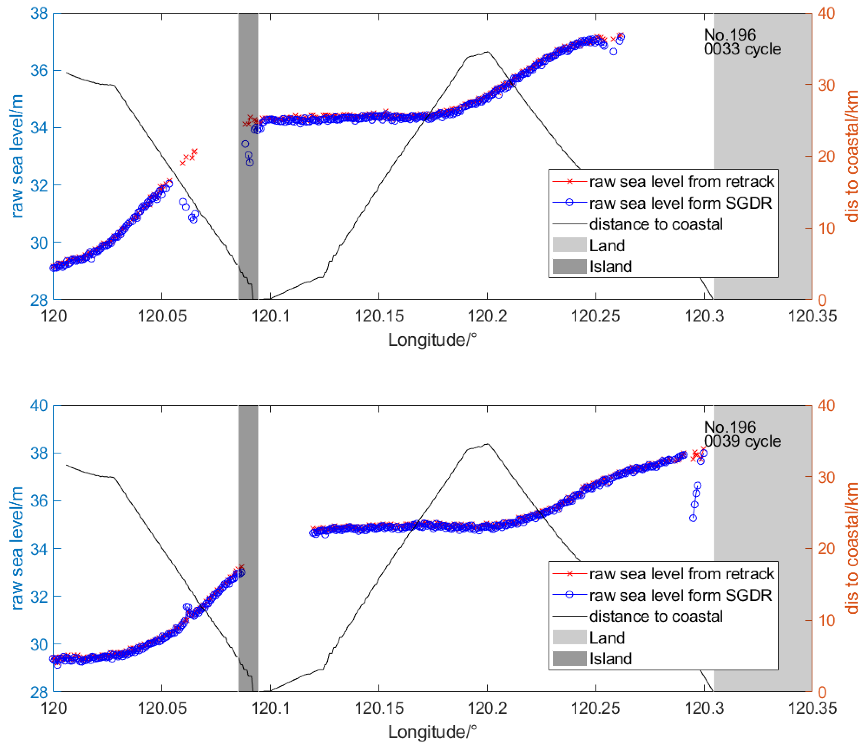
In the formula, the tracking range corresponds to the variable named tracker_20hz_ku in SGDR data, the retracking range correction is provided by the reprocessing of waveform retracking mentioned in Section 3, and the instrumental corrections mainly include the three variables named net_instr_corr_range_ku, cog_corr and modeled_instr_corr_range_ku in the SGDR data. The retracking range corresponds to the range_20hz_ku in SGDR data. The comparing results are shown in Figure 12 and Figure 13.
Figure 12 shows the RSL comparisons of the reprocessing results and the SGDR data in the pass 323. From Figure 12, it can be seen that the RSL of the reprocessing results and the SGDR data have the same trend of sea level change, but the sea surface height of reprocessing results is slightly higher than the SGDR data, which is mainly generated by the waveform noise caused by the circumstances that the trajectory of the pass 323 is parallel to the shoreline. The retracking strategy proposed in this study takes the noise into consideration and addresses this problem by determining the effective trailing edge. Hence, the reprocessing results are affected less. At 76.05°E, the distorting waveform caused by the high-energy reflection from coastal ‘contamination’ leads to a large RSL bias derived from the MLE4 tracker. The reprocessing results are not affected by this distortion of the waveform and still provide steady RSL data until approximately 10 km offshore.
Figure 13 shows the RSL comparisons of the reprocessing results and the SGDR data in the pass 196. Since the trajectory of the pass 196 is almost perpendicular to the shoreline, the satellite altimetry is slightly affected by the coastal land in theory. Hence, the RSL values of the reprocessing results and SGDR data are almost the same beyond 10 km offshore. Within 10 km offshore, a small amount of the RSL of the SGDR data deviates and has been corrected in the reprocessing results, especially in the range from 5 km to the island.
In summary, the waveform retracking proposed in this paper can process the near-shore waveform more accurately than the standard process applied in the SGDR data. In the range within 15 km offshore, the altimetry data are improved qualitatively and have retrieved more valid observations that are always thought to be outliers to the SGDR data.

5. Discussion

To quantitatively analyze the reliability and accuracy of the reprocessed high frequency data, the absolute sea surface height (ASSH) data of the reprocessed data and the SGDR data in pass 323 and pass 196 are compared with the tide gauge data. The ASSH is calculated as follows:
a b s o l u t e   s e a   l e v e l   h e i g h t a l t i m e t e r = a l t i t u d e r e t r a c k e d   r a n g e ( d r y   t r o p o s p h e r i c   c o r r c t i o n + w e t   t r o p o s p h e r i c   c o r r e c t i o n + i o n o s p h e r i c   c o r r e c t i o n )
a b s o l u t e   s e a   l e v e l   h e i g h t T G = s e a   l e v e l
The ASSH represents the sea surface height relative to the reference ellipsoid, which combines the effect of ocean tides and atmospheric forcing. The tide gauge data contain complete tidal information, so it is not necessary to remove the tide signal from the altimetry data. The tide gauge data do not correct the forcing of the dynamic atmosphere on the sea surface, so altimetry data do not correct the effect of atmospheric forcing. Since altimeters and tide gauges have different references, the mean difference between altimetry data and tide gauge data is removed when compared with each other. In addition, there is no sea state bias (SSB) correction in the ASSH because the SSB correction (low frequency) provided by the SGDR cannot support the high frequency data completely [33,34,35], and the SSB correction calculated by the inaccurate waveform retracking product in SGDR data is relatively inaccurate. By the way, once the wet tropospheric correction or the ionospheric correction provided by the instrument is lacking, the corrections provided models are adopted, which may lead an extra bias.
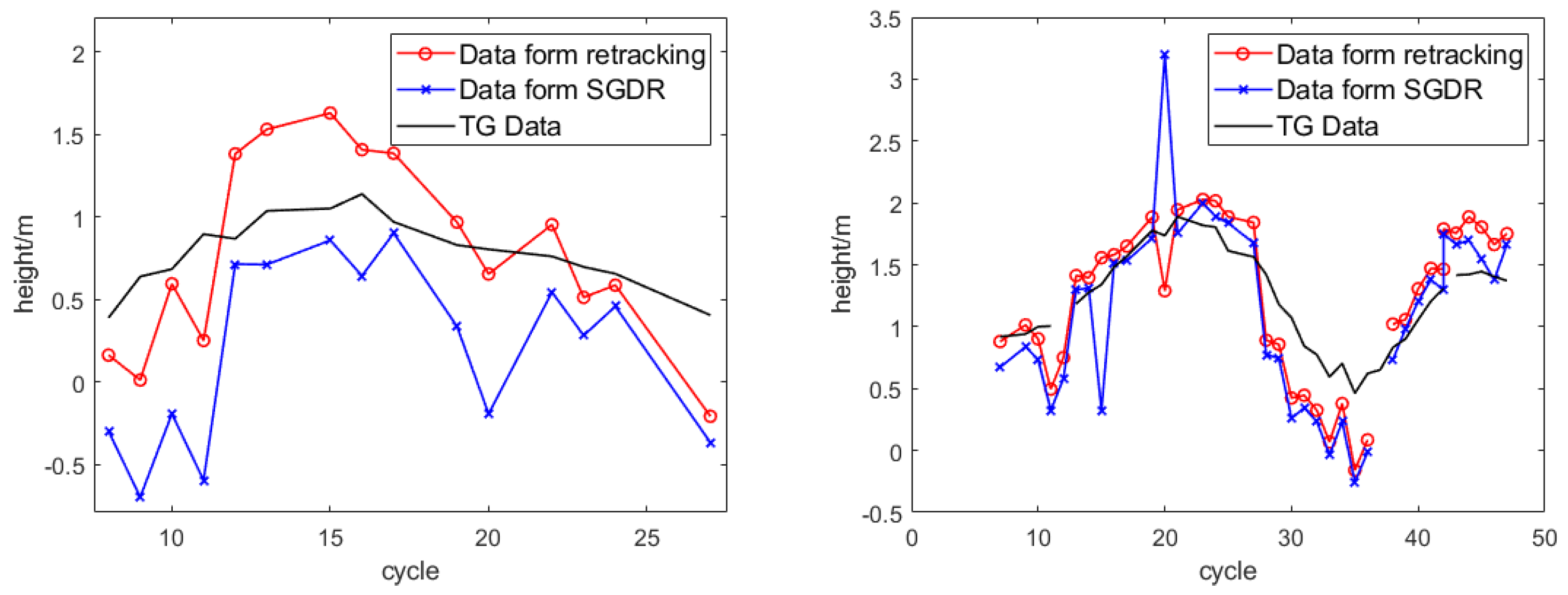
Before the quantitative analysis, we directly compare the height of altimetry data with the tide gauge data. According to the Section 4, the data within the range where the reprocessed data and SGDR data are obviously different are selected to calculate a range average of per cycle of two passes, the result is showed in Figure 14. The systemic height difference between HY-2B altimetry ASSH data and tide gauge data is removed.
From Figure 14, we can see that the changing of tide gauge observation and altimetry data are roughly same, and that the local trend is different due to the tide gauge does not completely fall into the trajectory of satellite. As stated in Section 4, the sea surface height of reprocessed data is higher than the SGDR data, and reprocessed data possesses more similar changes with the tide gauge data. In the comparison result of pass 323, the changing trend of cycle 13–17 of reprocessed data has better consistency with the tide gauge data than the SGDR data. Additionally, in the comparison result of pass 196, the SGDR data has more outliers, such as the value of cycle 15 and cycle 20, and the changing trend of cycle 40–50 of reprocessed data is more stable and coherent against tide gauge data.
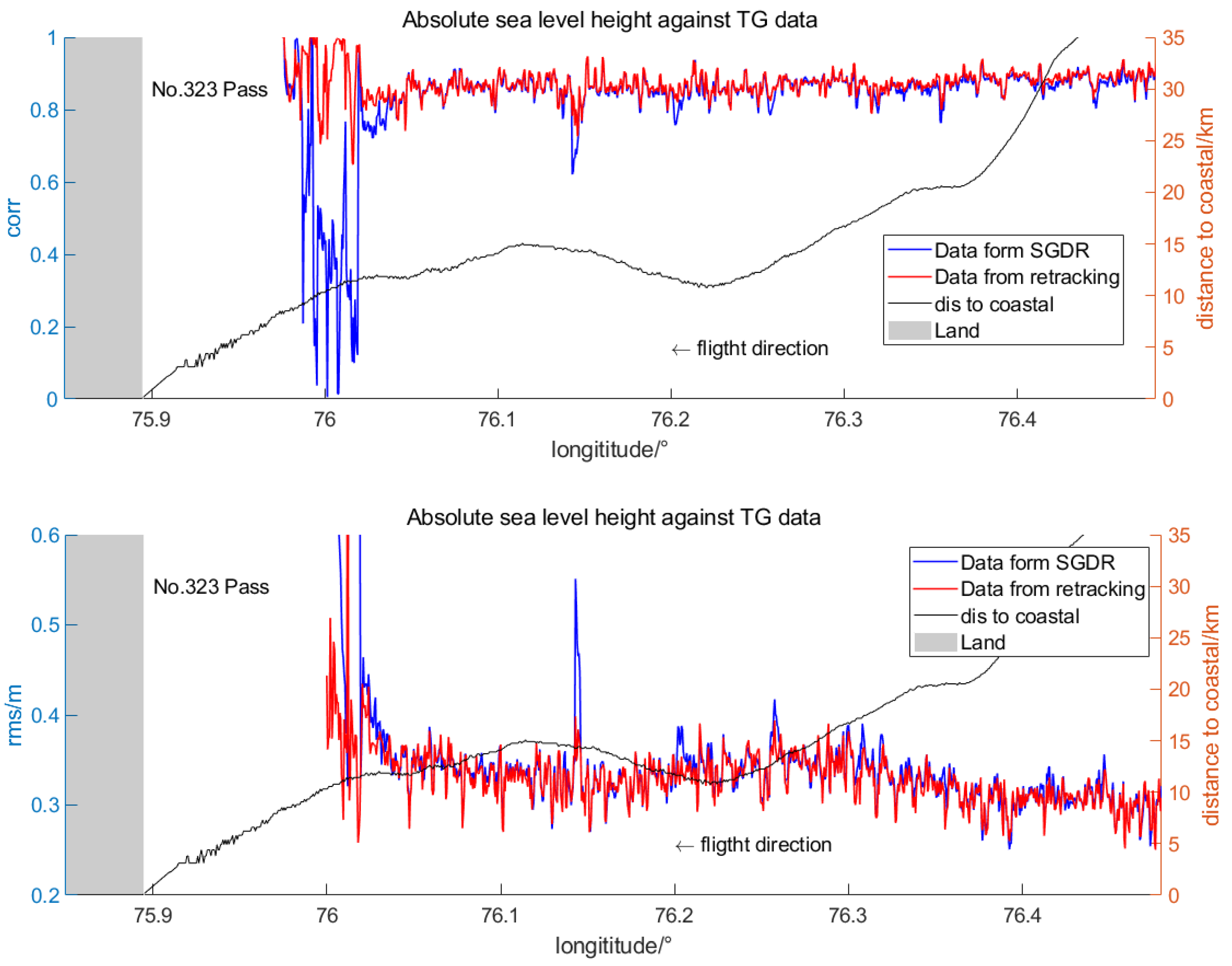
Then, based on the comparison method mentioned by Fenoglio [36], the different periods of the pass 323 and pass 196 data are linearly interpolated into the reference track, which consists of the normal points (NPs). Depending on the ASSH time series, the correlation coefficient and the root mean square (RMS) of reprocessing results and SGDR data against tide gauge data are calculated at each NP. The calculation results are shown in Figure 15 and Figure 16.
Figure 15 shows the correlation coefficient and RMS of the ASSH data against the tide gauge data in HY-2B pass 323. The correlation coefficient and RMS of the reprocessing results are basically better than those of the SGDR data. The correlation coefficient of reprocessing results beyond 20 km offshore is slightly higher than the SGDR data, and the RMS is maintained at approximately 30 cm. At distances between 13 km and 20 km from the shoreline, the correlation coefficient and RMS of the reprocessing results are the same as those of the SGDR data. The mean values of the correlation coefficient and RMS of the reprocessing results are 0.86 and 33.6 cm, and 0.86 and 34.0 cm for the SGDR data. The SGDR data are no longer reliable in the area within 12 km offshore, and the correlation coefficient and RMS worsen dissimilarly. Although the reprocessing results are influenced by the waveform noise caused by coastal land, the reprocessing results still show good performance, and the mean values of the correlation coefficient and RMS are 0.89 and 45.1 cm, respectively.
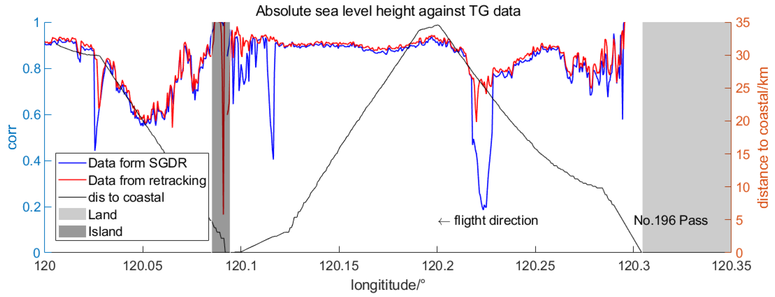
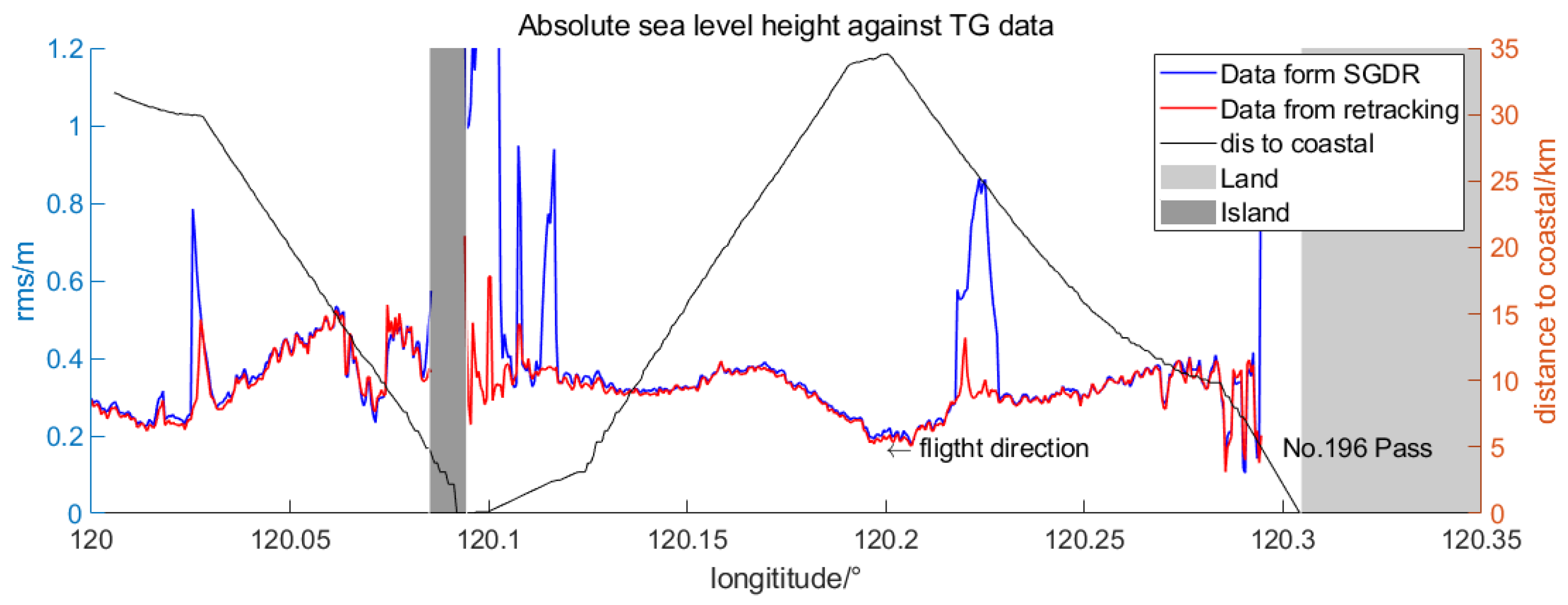
Figure 16 shows the correlation coefficient and RMS of the ASSH data against the tide gauge data in HY-2B pass 196. As shown in Figure 16, the quality of the reprocessing result is significantly improved compared to the SGDR data. The correlation coefficient of the reprocessing result has a steady and overall enhancement, and the mean values of the correlation coefficient and RMS are 0.90 and 29.3 cm in the range from 120.2°E to 120.125°E. In contrast, the mean values of the correlation coefficient and RMS of the SGDR data are 0.89 and 30.0 cm, respectively. This is attributed to the effective trailing edge processing of waveform retracking, which can not only address the distortion of the waveform but also weaken the influence of trailing edge noise. In the range of 12 km offshore, although the correlation coefficient and RMS of the reprocessing results are better than those of the SGDR data, they fluctuate due to the observation mode conversion of the altimeter, and the mean values of the correlation coefficient and RMS for the reprocessing data are 0.84 and 33.0 cm, respectively. Within the range 5 km offshore (120.125°E to 120.09°E), the data quality of the SGDR products worsens as the shoreline approaches, and the reprocessing results show high quality, with mean values of the correlation coefficient and RMS of 0.92 and 36.2 cm, respectively, which is similar to the open sea observations. This also illustrates that the waveform retracking provided in this study is good at dealing with the waveform influenced by some small coastal ‘pollution’, such as coastal islands.
According to the above analysis, the reliability and accuracy of the HY-2B altimetry data processed by waveform retracking proposed in this study are better than those of the standard SGDR data in coastal areas. In the range beyond 20 km from the shoreline, the correlation coefficient and RMS of the reprocessing results are slightly better than those of the SGDR data, which indicates that the waveform retracking proposed in this study is also suited to open sea observations. Within 15 km offshore, the precision of SGDR data decreases seriously, while the reprocessing results are still fine advancing the application potential of HY-2B satellite altimetry data in coastal areas.

6. Conclusions

To solve the problem that the accuracy of HY-2B satellite altimetry data decreases and the available data reduces in costal area, a coastal waveform retracking strategy for HY-2B altimetry is proposed. The coastal waveform of the HY-2B satellite altimeter is retracked by determining the effective trailing edge and the leading edge, which is less affected by coastal ‘pollution’. The coastal waveform data of pass 323 and pass 196 are reprocessed to validate the performance of the proposed waveform retracking strategy by comparing the reprocessing results to the SGDR data and tide gauge observations, and the results are verified qualitatively and quantitatively in the study areas.
The altimeter waveform is distorted by coastal ‘pollution’ in coastal areas, such as land or bright targets over the sea. Based on a certain criterion, the waveform retracker proposed in this study detects the leading edge of the waveform, which contains less noise, looks for the effective part of the trailing edge, and then corrects the waveform fitting bias due to the coastal distorted waveform. The proposed waveform retracker avoids careful waveform classification and the boundary demarcation between open sea and coastal areas. The potential application of HY-2B satellite altimeter data in coastal areas is improved under the condition that the accuracy of open sea observations is retained.
According to the analysis of the reprocessing results against TG data and SGDR data, the data quality of the reprocessing results is basically better than that of the SGDR data, especially in the range within 15 km offshore. For the reprocessing result of the pass 323 data, the mean correlation coefficient and RMS are 0.89 and 45.1 cm within 12 km offshore, respectively, while the SGDR data are mostly invalid, with a correlation coefficient lower than 0.5 and an RMS greater than 60 cm. The reprocessing result of pass 196 data also maintains high quality, with a mean correlation coefficient and RMS of 0.92 and 36.2 cm, respectively, in the range within 5 km offshore, which is almost consistent with the quality of open sea observations. All of the above results show that the waveform retracker proposed in this study has good performance in coastal areas.
Waveform retracking is the first step for the coastal altimetry data reprocessing, extra processes are needed, such as the recalculation of high frequency SSB, the recalculation of coastal wet tropospheric correction, the filtering of ionospheric correction, and the improvement of tide model, etc. After that, the high quality coastal altimetry data is obtained and applied into practice.

Author Contributions

Z.H. and J.Y. proposed and designed the technique route. C.F. gave advice about the implementation of technology. Z.H. reprocessed the waveform data. J.Y., Y.J. and W.C. helped with analysis of reprocessed data. Z.H., J.Y., W.C. and S.L. reviewed the manuscript. All authors have read and agreed to the published version of the manuscript.

Funding

This research was funded by the National Natural Science Foundation of China under Grant No. 42106178, the Basic Scientific Fund for National Public Research Institutes of China under Grant No. 2020Q07, ESA-MOST CHINA Dragon 5 Programme under Grant No. 58900, and Science Foundation of Donghai Laboratory.

Acknowledgments

The author would like to thank the National Satellite Ocean Application Service and University of Hawaii Sea Level Center provided the measurement data of altimeter and tide gauge, and all researchers who assisted us in studying.

Conflicts of Interest

The authors declare no conflict of interest.

References

  1. Brown, G. The average impulse response of a rough surface and its applications. IEEE Trans. Antennas Propag. 1997, 25, 67–74. [Google Scholar] [CrossRef]
  2. Hayne, G.S. Radar altimeter mean return waveforms from near-normal-incidence ocean surface scattering. IEEE Trans. Antennas Propag. 1980, 28, 687–692. [Google Scholar] [CrossRef] [Green Version]
  3. Martin, T.V.; Zwally, H.J.; Brenner, A.C. Analysis and retracking of continental ice sheet radar altimeter waveforms. J. Geophys. Res. Ocean. 1983, 88, 1608–1616. [Google Scholar] [CrossRef]
  4. Wingham, D.J.; Raplet, C.G.; Griffiths, H. New techniques in satellite tracking system. In Proceedings of the IGARSS’86 Symposium, Zurich, Switzerland, 8 September 1986; pp. 1339–1344. [Google Scholar]
  5. Davis, C.H. A robust threshold retracking algorithm for measuring ice-sheet surface elevation change from satellite radar altimeters. IEEE Trans. Geosci. Remote Sens. 1997, 35, 974–979. [Google Scholar]
  6. Hwang, C.; Guo, J.; Deng, X.; Hsu, H.Y.; Liu, Y. Coastal gravity anomalies from retracked GEOSAT/GM altimetry: Improvement, limitation and the role of airborne gravity data. J. Geod. 2006, 80, 204–216. [Google Scholar] [CrossRef]
  7. Sandwell, D.T.; Smith, W. Retracking RES-1 altimeter waveforms for optimal gravity field recovery. Geophys. J. R. Astron. Soc. 2005, 163, 79–89. [Google Scholar] [CrossRef] [Green Version]
  8. Quartly, G.D.; Smith, W.H.F.; Passaro, M. Removing Intra-1-Hz Covariant Error to Improve Altimetric Profiles of σ0 and Sea Surface Height. IEEE Trans. Geosci. Remote Sens. 2019, 57, 3741–3752. [Google Scholar] [CrossRef]
  9. Passaro, M.; Cipollini, P.; Vignudelli, S.; Quartly, G.D.; Snaith, H.M. ALES: A multi-mission adaptive subwaveform retracker for coastal and open ocean altimetry. Remote Sens. Environ. 2014, 145, 173–189. [Google Scholar] [CrossRef] [Green Version]
  10. Passaro, M.; Fenoglio-Marc, L.; Cipollini, P. Validation of significant wave height from improved satellite altimetry in the german bight. IEEE Trans. Geosci. Remote Sens. 2015, 53, 2046–2156. [Google Scholar] [CrossRef]
  11. Birol, F.; Léger, F.; Passaro, M.; Cazenave, A.; Benveniste, J. The X-TRACK/ALES multi-mission processing system: New advances in altimetry towards the coast. Adv. Space Res. 2021, 67, 2398–2415. [Google Scholar] [CrossRef]
  12. Dettmering, D.; Müller, F.L.; Oelsmann, J.; Passaro, M.; Seitz, F. North SEAL: A new dataset of sea level changes in the North Sea from satellite altimetry. Earth Syst. Sci. Data 2021, 13, 3733–3753. [Google Scholar] [CrossRef]
  13. Arabsahebi, R.; Voosoghi, B.; Tourian, M.J. The Inflection-Point Retracking Algorithm: Improved Jason-2 Sea Surface Heights in the Strait of Hormuz. Mar. Geod. 2018, 41, 331–352. [Google Scholar] [CrossRef]
  14. Roscher, R.; Uebbing, B.; Kusche, J. STAR: Spatio-temporal altimeter waveform retracking using sparse representation and conditional random fields. Remote Sens. Environ. 2017, 201, 148–164. [Google Scholar] [CrossRef] [Green Version]
  15. Schlembach, F.; Passaro, M.; Quartly, G.D.; Kurekin, A.; Donlon, C. Round Robin Assessment of Radar Altimeter Low Resolution Mode and Delay-Doppler Retracking Algorithms for Significant Wave Height. Remote Sens. 2020, 12, 1254. [Google Scholar] [CrossRef] [Green Version]
  16. Wang, X.; Ichikawa, K.; Wei, D. Coastal Waveform Retracking in the Slick-Rich Sulawesi Sea of Indonesia Based on Variable Footprint Size with Homogeneous Sea Surface Roughness. Remote Sens. 2019, 11, 1274. [Google Scholar] [CrossRef] [Green Version]
  17. Quartly, G.D. Determination of Oceanic Rain Rate and Rain Cell Structure from Altimeter Waveform Data. J. Atmos. Ocean. Technol. 1998, 15, 1361–1378. [Google Scholar] [CrossRef]
  18. Quartly, G.D. Hyperbolic Retracker: Removing Bright Target Artefacts from Altimetric Waveform Data. In ESA SP-686, Living Planet Symposium; ESA Publication: Bergen, Norway, 2010; SP-686. [Google Scholar]
  19. Tournadre, J. Signature of lighthouses, ships, and small islands in altimeter waveforms. J. Atmos. Ocean. Technol. 2007, 24, 1143–1149. [Google Scholar] [CrossRef]
  20. Wang, X.; Ichikawa, K. Coastal Waveform Retracking for Jason-2 Altimeter Data Based on Along-Track Echograms around the Tsushima Islands in Japan. Remote Sens. 2017, 9, 762. [Google Scholar] [CrossRef] [Green Version]
  21. Peng, F.; Deng, X. A new retracking technique for Brown peaky altimetric waveforms. Mar. Geod. 2017, 41, 99–125. [Google Scholar] [CrossRef]
  22. Peng, F.; Deng, X. Validation of Sentinel-3A SAR mode sea level anomalies around the Australian coastal region. Remote Sens. Environ. 2020, 237, 111548. [Google Scholar] [CrossRef]
  23. Deng, X.; Featherstone, W.E. A coastal retracking system for satellite radar altimeter waveforms: Application to ERS-2 around Australia. J. Geophys. Res. Ocean. 2006, 111, 95. [Google Scholar] [CrossRef]
  24. Yang, L.E.; Lin, M.; Liu, Q.; Pan, D. A coastal altimetry retracking strategy based on waveform classification and sub-waveform extraction. Int. J. Remote Sens. 2012, 33, 7806–7819. [Google Scholar] [CrossRef]
  25. Nurul, I.; Xiaoli, D.; Ami, M.D.; Nurul, I. CAWRES: A Waveform Retracking Fuzzy Expert System for Optimizing Coastal Sea Levels from Jason-1 and Jason-2 Satellite Altimetry Data. Remote Sens. 2017, 9, 603. [Google Scholar]
  26. Peng, F.; Deng, X.; Cheng, X. Quantifying the precision of retracked Jason-2 sea level data in the 0–5 km Australian coastal zone. Remote Sens. Environ. 2021, 263, 112539. [Google Scholar] [CrossRef]
  27. Jia, Y.; Yang, J.; Lin, M.; Zhang, Y.; Fan, C. Global Assessments of the HY-2B Measurements and Cross-Calibrations with Jason-3. Remote Sens. 2020, 12, 2470. [Google Scholar] [CrossRef]
  28. Amarouche, L.; Thibaut, P.; Zanife, O.Z.; Dumont, J.P.; Vincent, P.; Steunou, N. Improving the Jason-1 ground retracking to better account for attitude effects. Mar. Geod. 2004, 27, 171–197. [Google Scholar] [CrossRef]
  29. Poisson, J.C.; Ouartly, G.D.; Kurekin, A.A.; Thibaut, P.; Hoang, D.; Nencioli, F. Development of an ENVISAT altimetry processor providing sea level continuity between open ocean and Arctic leads. IEEE Trans. Geosci. Remote Sens. 2018, 56, 5299–5319. [Google Scholar] [CrossRef]
  30. Halimi, A.; Mailhes, C.; Tourneret, J.Y.; Thibaut, P.; Boy, F. Parameter estimation for peaky altimetric waveforms. IEEE Trans. Geosci. Remote Sens. 2013, 51, 1568–1577. [Google Scholar] [CrossRef]
  31. Peacock, N.R.; Laxon, S.W. Sea surface height determination in the Arctic ocean from ERS altimetry. J. Geophys. Res. Ocean. 2004, 109, 120. [Google Scholar] [CrossRef]
  32. Chelton, D.B.; Walsh, E.J.; Macarthur, J.L. Pulse compression and sea level tracking in satellite altimetry. J. Atmos. Ocean. Technol. 1989, 6, 407–438. [Google Scholar] [CrossRef]
  33. Cipollini, P.; Calafat, F.M.; Jevrejeva, S.; Melet, A.; Prandi, P. Monitoring Sea Level in the Coastal Zone with Satellite Altimetry and Tide Gauges. Surv. Geophys. 2017, 38, 33–57. [Google Scholar] [CrossRef] [PubMed] [Green Version]
  34. Passaro, M.; Nadzir, Z.A.; Quartly, G.D. Improving the precision of sea level data from satellite altimetry with high-frequency and regional sea state bias corrections. Remote Sens. Environ. 2018, 218, 245–254. [Google Scholar] [CrossRef]
  35. Peng, F.; Deng, X. Improving precision of high-rate altimeter sea level anomalies by removing the sea state bias and intra-1-Hz covariant error. Remote Sens. Environ. 2020, 251, 112081. [Google Scholar] [CrossRef]
  36. Fenoglio-Marc, L.; Fehlau, M.; Ferri, L.; Becker, M.; Bao, Y.; Vignudelli, S. Coastal sea surface heights from improved altimeter data in the Mediterranean Sea. Gravity Geoid Earth Obs. 2010, 135, 253–261. [Google Scholar]
Figure 1. The diagrammatic sketch of an ideal waveform based on Brown model.
Remotesensing 14 05026 g001
Figure 2. The study areas and the ground track of HY-2B altimeter (red lines respectively indicate the trajectory of pass 323 (A) and the trajectory of pass 196 (B), the yellow blocks are the tide gauge stations and the shadow represents coastal land).
Remotesensing 14 05026 g002
Figure 3. The examples of real waveform with small mispointing angle (The left is the sharpening waveform and the right is the specular waveform).
Remotesensing 14 05026 g003
Figure 4. Flow diagram of coastal waveform retracking procedure of HY-2B altimetry.
Remotesensing 14 05026 g004
Figure 5. Examples of the first kind of “possible ending gate of leading edge”, the x-axis is the number of gate and the y-axis is the normalized power of echo. The blue line is whole waveform, the red line is the leading edge depending on the “normal ending gate of leading edge”, the marked yellow gate is the first kind of “possible ending gate of leading edge” with increasing power.
Remotesensing 14 05026 g005
Figure 6. Examples of the second kind of “possible ending gate of leading edge”, the x-axis is the number of gate and the y-axis is the normalized power of echo. The blue line is whole waveform, the red line is the leading edge depending on the “normal ending gate of leading edge”, the yellow gate marked is the second kind of “possible ending gate of leading edge” with decreasing power.
Remotesensing 14 05026 g006
Figure 7. Examples of the invalid “possible ending gate of leading edge”.
Remotesensing 14 05026 g007
Figure 8. Flow diagram of effective trailing edge search.
Remotesensing 14 05026 g008
Figure 9. The distortion of trailing edge judged by the fitting-straight line, the x-axis is the number of gate and the y-axis is the normalized power of echo. The blue line is real waveform and green line is the fitting-straight line, the red line circles the distortion. (a) the “convex” caused by one distortion of trailing edge against straight line; (b) the “concave” caused by two distortions of trailing edge against straight line.
Remotesensing 14 05026 g009aRemotesensing 14 05026 g009b
Figure 10. The effective trailing edge search. the x-axis is the number of gate and the y-axis is the normalized power of echo, the blue line is real waveform and red line is the effective trailing edge.
Remotesensing 14 05026 g010
Figure 11. The fitting results of real waveforms.
Remotesensing 14 05026 g011
Figure 12. The RSL comparisons between the reprocessing results and SGDR data of pass 323 (x-axis is the along-track latitude, the left y-axis is the RSL and the right y-axis is the distance from the nominal points of the track to the shoreline illustrated by the black line, the blue line is the SGDR data and red line is the reprocessing results. The light shadow area represents the land; the direction of flight is from 76.5° to 75.9°).
Remotesensing 14 05026 g012aRemotesensing 14 05026 g012b
Figure 13. The RSL comparisons between the reprocessing results and SGDR data of pass 196 (x-axis is the along-track latitude, the left y-axis is the RSL and the right y-axis is the distance from the nominal points of the track to the shoreline illustrated by the black line, the blue line is the SGDR data and red line is the reprocessing results. The light shadow area represents the land and deep shadow area represents the coastal island, the direction of flight is from 120.35° to 120°).
Remotesensing 14 05026 g013aRemotesensing 14 05026 g013b
Figure 14. Height comparison of the ASSH between HY-2B pass 323 and pass 196 with tide gauge data. (x-axis is the number of cycle. The y-axis is the unified value of sea surface height. The left is the comparison within the range 10 km offshore for pass 323, the right is the comparison within the range from 10 km to the island for pass 196).
Remotesensing 14 05026 g014
Figure 15. Correlation coefficient (top) and RMS (bottom) of the ASSH data comparing with tide gauge data of Subic Bay Station for HY-2B pass 323; (x-axis is the along-track latitude of the nominal tracks. The shaded light grey indicates the land).
Remotesensing 14 05026 g015
Figure 16. Correlation coefficient (top) and RMS (bottom) of the ASSH data comparing with tide gauge data of Subic Bay Station for HY-2B pass 196; (x-axis is the along-track latitude of the nominal tracks. The shaded light grey indicates the land and the deep shadow represents coastal island).
Remotesensing 14 05026 g016aRemotesensing 14 05026 g016b
Publisher’s Note: MDPI stays neutral with regard to jurisdictional claims in published maps and institutional affiliations.