Abstract
Temperature lapse rate (TLR) is an important parameter for simulations of snow/glacier melts in alpine watersheds. However, the traditional scheme estimates TLR mainly based on a limited number of stations and may not be suitable for alpine watersheds with scarce observations. To overcome this problem, this study developed a new basin-oriented TLR scheme based on Moderate Resolution Imaging Spectroradiometer (MODIS) land surface temperature data which was applied in a typical glacierized watershed on the northern slope of the Himalayas. The new TLR scheme was evaluated by comparison with the station-based traditional TLR scheme in terms of performance in simulations of both snow cover area and runoff using the same hydrological model. The results showed that the monthly TLRs estimated by the new scheme presented a more reasonable seasonal pattern than those estimated by the traditional scheme. The model using the new TLR scheme showed better performance in discharge simulations of low-runoff months than that using the traditional TLR scheme. The R-squared value of multiyear mean monthly snow cover area of the former (0.82) was also higher than that of the latter (0.56). This study provides an efficient framework for estimating TLR based on remote sensing for alpine watersheds with scarce observations.
1. Introduction
The Tibetan Plateau, with an average altitude of more than 4000 m, is the birthplace of more than a dozen rivers in Asia [1]. It supports more than one-sixth of the world’s population and is known as the world’s water tower [2]. The Tibetan Plateau provides water, pasture and other resources to more than a dozen bordering countries, affecting about 2 billion people [3]. Since snow and glaciers exist year-round at high elevations of the Tibetan Plateau, glacier and snow melts are important factors affecting the runoff changes of the upstream river basins [4]. For example, it is reported that snowmelt contributes more than 20% of the total runoff to the upper basins of six major rivers on the Tibetan Plateau, and the glacier melts account for 40% to over 50% of the total runoff in the upper Indus River basin [5,6,7]. Therefore, it is important to accurately simulate glacier-melt and snow-melt runoff, which would lead to a better understanding of hydrological processes of the Tibetan Plateau and contribute to flood forecasting and water resource management in downstream areas [8,9].
The hydrological models that incorporate snow or glacier modules are widely used to simulate the changes of glacier-melt and snow-melt runoff in alpine basins. Such models can be mainly divided into two categories, namely the temperature index method based on an empirical relationship of glacier/snow melt and temperature [10,11] and the energy balance method [12]. The energy balance method, such as the DHSVM model [13], WEB-DHM-S model [14] and the GBEHM model, fully considers the main physical processes involved in snow and glacier change and can reasonably quantify and distinguish their important components (e.g., sublimation) [15,16]. However, the energy balance method has high requirements for input data such as the hourly radiation and humidity, which are generally difficult to obtain in an alpine basin with sparse meteorological observations. As it requires only daily temperature and precipitation data, the temperature index method, such as the J2000 model [17,18], SRM model [19] and SPHY model [20], has been widely used in the simulation of glacier and snow melt in global alpine basins [5,21].
Though model structure has an important effect on the simulations, the meteorological inputs have been recently identified as major error sources for snow modeling on the Tibetan Plateau based on evaluations of multiple reanalysis datasets and global climate models [22,23]. As a key factor of glacier/snow melting, air temperature is an important input for hydrological modeling in alpine basins [24,25]. However, due to the complex topography and harsh climate, meteorological stations with long-term continuous observations are scarce and mostly located in the eastern part of the Tibetan Plateau with lower elevations. To obtain the spatial and temporal variation of air temperature in the high-altitude region, previous studies often employed air temperature interpolations based on a limited number of meteorological stations in hydrological models [26]. One of the most commonly used methods for interpolating air temperature is the temperature lapse rate (TLR) method, which assumes that temperature decreases at a constant rate with increasing elevation. The global reference TLR is −0.65 °C/100 m, which means that air temperature decreases by an average of 0.65 °C with an elevation increase of 100 m. TLR is widely used in spatial interpolation of air temperature data for considering the elevation differences between the stations and model grids [6,27,28]. It is also an important parameter inherently used in various hydrological models for applications in alpine basins [17,29]. A fixed TLR of 0.65 °C/100 m was frequently used in previous studies [30,31]; however, TLR actually varies with climatic conditions, geographical location, topographic features and land cover types [32]. Since TLR is usually estimated from station observations, the problem of sparse stations also severely limits the accurate estimation of TLR on the Tibetan Plateau.
To address the problem of scarce temperature observations, recent studies have estimated air temperature over the Tibetan Plateau [33,34] based on remote sensing land surface temperature (LST) from various sensors such as Landsat OLI-ETM+ [35] and Moderate Resolution Imaging Spectroradiometer (MODIS) [36]. For example, MODIS data have been widely used in exploring the spatiotemporal changes of various environmental variables [37] including LST changes and their relationship with other factors in mountainous regions of the Himalayas [38]. The MODIS LST data were also used as predictors in artificial intelligence (AI) and machine learning (ML) models for forecasting snow cover and vegetation changes [39]. Although air temperature is not equivalent to LST, air temperature lapse rate is found to have a strong spatial and temporal consistency with LST lapse rate [40]. Therefore, MODIS LST data have recently been directly used to estimate the TLR, showing relatively good accuracy [41,42]. Currently, there are few studies evaluating the feasibility of remote sensing TLR in hydrological simulations in alpine basins. It is demonstrated that the monthly TLRs estimated from MODIS nighttime LST can significantly improve the accuracy of snow dynamics simulations in the Upper Yellow River Basin compared to those obtained from sparse stations [43]. However, the high cloud cover greatly limits the applicability of remote sensing TLR and frequently causes abnormal TLR values (e.g., absolute TLR > 1.5 °C/100 m) [44]. In addition, there is no glacier-melt runoff in the study area, and previous studies [43,44,45] mainly focused on producing remote sensing TLRs at rectangular grids and coarse resolutions, which are not suitable for meso- and micro-scale alpine basins with an irregular shape. Thus, it is urgent to develop an efficient parameterization scheme of TLR for hydrological simulation that can alleviate the problem of cloud coverage and to further evaluate the feasibility of remote sensing TLR in hydrological simulations in glacierized basins.
The objectives of this study were: (1) to develop a new parameterization scheme of TLR based on remote sensing LST, which is basin-oriented; (2) to apply the new TLR scheme in the hydrological simulation in a typical glacierized basin of the Tibetan Plateau; (3) to evaluate the feasibility of the new TLR scheme by comparing with the station-based TLR in terms of the accuracy of both runoff and snow simulations.
2. Materials and Methods
2.1. Study Area
In this study, the Karuxung watershed (Figure 1), which originates from the northern slope of the Himalayas, was selected as the study area. The watershed is in the southern part of the Tibet Autonomous Region, China, with latitude and longitude ranges from 28°46′19″N to 29°0′22″N and 90°8′8″E to 90°23′4″E, respectively. The watershed area is 286 km2, and the elevation range varies from a minimum elevation of 4550 m at Wengguo hydrological station to a maximum of 7200 m. A total of 50 glaciers in the basin cover a total area of 47 km2.
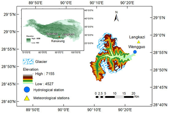
Figure 1.
Location and topography of the study area (i.e., the Karuxung watershed).
2.2. Observation Data
Meteorological data from two stations were used here. The meteorological station nearest to the Karuxung watershed is the Langkazi station with an altitude of 4432.4 m and has daily meteorological observations (including daily minimum air temperature, maximum air temperature, average air temperature, precipitation, relative humidity, sunshine duration and average wind speed) from 1980 to present. The second nearest one is the Gyantse station, which is 78 km away at an altitude of 4040 m. The Gyantse station has daily meteorological data from 1956 to present. The annual average temperature of the Langkazi meteorological station from 1985 to 2014 is 3.3 °C. The multi-year average annual precipitation, including rainfall and snowfall, is 379.9 mm, with June to September accounting for 90% of the annual precipitation. Most of the precipitation from October to March is in the form of snowfall, which lasts longer at higher altitudes.
Daily runoff observations were obtained from the Wengguo hydrological station. The runoff data are available for 1 January 1985 to 31 December 1994 and 1 April 2006 to 31 December 2014. For evaluation of snow cover and runoff simulations, the years 1985–1994 were selected as the model calibration period and April 2006 to December 2014 as the model validation period based on data availability (Table 1).

Table 1.
Daily observation data used for model input, calibration and validation.
2.3. Remote Sensing Data
MODIS TERRA daily LST data collection 6 (MOD11A1) was used for developing the new TLR scheme (Section 2.4.2). MODIS TERRA provides LST data of two overpass times including one daytime LST (at about 10:30 am) and one nighttime LST (at about 10:30 pm). The nighttime LST data were used here because MODIS nighttime LST showed better performance in estimating monthly TLR for the Tibetan Plateau than the daytime LST [40]. The land cover type data from MODIS (MOD12Q1) were used for identifying water pixels, which were excluded in the process of TLR estimation based on MODIS LST (Section 2.4.2). The long time series data of daily snow cover area (SCA) on the Tibetan Plateau (2003–2014) were downloaded from National Tibetan Plateau/Third Pole Environment Data Center (data.tpdc.ac.cn) and were used for validating the snow simulations. The cloud-free daily snow cover data were created by combining MODIS daily snow cover data (from both Terra and Aqua) and the Interactive Multisensor Snow (IMS) product, with a spatial resolution of 0.005 degrees (approx. 500 m) [46]. An evaluation based on snow depth observations from 91 stations across the Tibetan Plateau showed that the overall accuracy of the cloud-free daily snow cover dataset is reported to be 92% [46]. By using nearest neighbor interpolation, 500 × 500 m pixels of the original snow cover data were resampled to 90 × 90 m to match the resolution of the digital elevation model data and to capture the snow at the watershed boundary more accurately. The 90 m digital elevation data of the Shuttle Radar Topography Mission (SRTM) were downloaded from the National Science Data Platform. Land use data at a scale of 1:1,000,000 including glacier distribution were obtained from the Northwest China Environmental and Ecological Science Data Center (http://westdc.westgis.ac.cn).
2.4. Methods
The entire workflow of this study is shown in Figure 2. Firstly, two parameterization schemes of monthly TLR were applied for the Karuxung watershed, namely the traditional method that estimates TLR based on station observations and a new scheme developed based on MODIS LST. Then, both TLR schemes were used to drive hydrological simulations of the Karuxung watershed, with the same settings of other model inputs; Lastly, the two schemes were evaluated and compared according to their performance in simulating runoff and snow cover. The detailed procedures are described in the following sections.
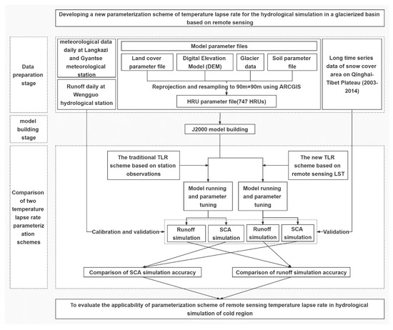
Figure 2.
The flowchart of methods used in this study. “HRU” means hydrological response unit; “SCA” means snow cover area.
2.4.1. The Traditional TLR Scheme Based on Station Observations
Previous studies found that TLR showed significant seasonal changes and estimated TLR mainly based on station observations [24]. As for the Karuxung River Basin, the multiyear-average monthly TLRs were estimated based on air temperature observations from two stations, namely Langkazi and Gyantse, and were then used to drive a snow-melt runoff model [8]. A similar scheme was adopted here. For both meteorological stations, multiyear-average monthly temperatures were calculated by temporally aggregating daily air temperature observations during the period of 1980–2014. Then, monthly TLR values were calculated based on the differences in elevation and multiyear-average monthly air temperature and between the two meteorological stations.
2.4.2. A New TLR Scheme Based on Remote Sensing LST
Previous studies found that the high cloud cover of the Tibetan Plateau resulted in many missing values and abnormal TLR estimates [45]. To address this problem and to better downscale the reanalysis air temperature data with coarse resolutions, an efficient method of dynamically checking the standard deviation of elevations within a coarse reanalysis grid has recently been employed [44]. Inspired by their study, a new TLR scheme that is oriented to basin scale was developed here. First, multiple ring buffers were created for the Karuxung watershed (Figure 3). The distance between buffers was set to 1 km, which is close to a pixel size of MODIS LST. The original extent of the watershed is considered as buffer No. 0, and the buffer number increases gradually from the inner watershed outwards with the maximum buffer number set to 18 here. This ensures that the area is not too large so as to avoid obvious effects from longitude or latitude [47]. Then, multiyear-average monthly mean LSTs were calculated for each of the MODIS LST pixels within all the buffers. The MODIS pixels containing water bodies were excluded, and only the MODIS pixels with temporal coverage > 1/2 were included in the calculation of TLR. The TLR calculation starts from the innermost buffer, which is the original polygon of the watershed (i.e., buffer No. 0). Before the TLR calculation, a dynamic checking procedure was applied following the method of Zhang [44], i.e., all the valid MODIS LST pixels within the buffer No. 0 were examined. If the standard deviation of elevations was less than 50 m or the correlation between LST and elevation was less than 0.5 or the percentage of valid pixels < 50%, the current buffer was considered unable to provide enough valid MODIS LST pixels to calculate a reliable TLR, and the calculation extended to the next buffer, meaning that the valid MODIS LST pixels within buffers No. 0 and No. 1 were included in the TLR calculation. This process was not stopped until the valid MODIS LST pixels could meet the requirements. It should be noted that the new TLR scheme also considers the location of the meteorological station. When the station is outside the watershed, the initial buffer was changed from buffer No. 0 to the No. of buffers where the station is located, e.g., for the Karuxung watershed, the Langkazi station is located in buffer No. 7, and the initial calculation involves the MODIS LST pixels within the areas of buffers Nos. 0–7. Once the No. of the final buffer for TLR calculation was determined, all the valid MODIS LST pixels of the related buffers were used to construct a linear regression between the monthly LST and elevation according to Equation (1).
where is the monthly average LST of each MODIS LST pixel involved, Z is the pixel elevation, a and b are the regression parameters and a is the estimated TLR. It should be noted that the abovementioned process was conducted for all 12 months. Finally, the 12-monthly TLR values were obtained for the Karuxung watershed.
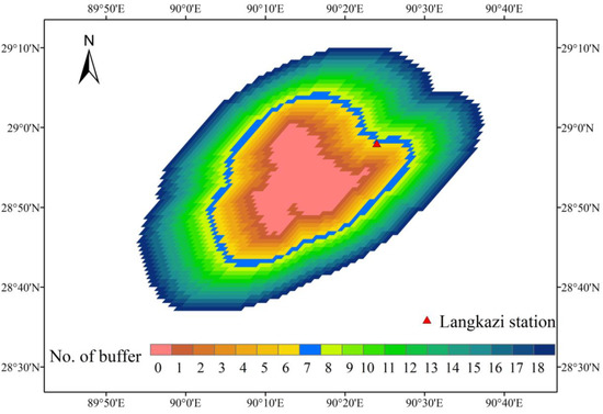
Figure 3.
Distribution of the multiple ring buffers used in the new TLR scheme. The pink region is the extent of the Karuxung watershed (i.e., buffer No. 0); The sky-blue region is buffer No. 7 where the Langkazi meteorological station located.
2.4.3. Hydrological Simulations
The monthly TLRs estimated using the two schemes were then used to drive hydrological simulations of Karuxung watershed based on the J2000 model (Figure 4). The J2000 model is a process-based hydrological model that considers major hydrological processes of the cryosphere such as interception, evaporation, snowmelt, glacier-melt, soil water, groundwater and sink flow [48]. The interception module of J2000 takes into account the maximum storage capacity of that vegetation for rain and snow based on the leaf area index of the vegetation type. The glacier-melt, snowmelt and rainfall are partially or fully infiltrated into the soil according to the infiltration rate of the soil (the maximum infiltration rate in summer, winter and with or without snow cover is determined by calibrating the parameters). Since this study focuses on improving TLR and the application in glacier/snow-melt simulations, descriptions about model inputs, glacier module and snow module are provided here. More details about other modules can be found in the user guide [49].
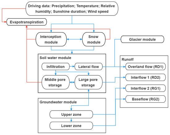
Figure 4.
The structure of the J2000 model.
In total, 747 hydrological response units (HRUs) were constructed in the Karuxung watershed. The model obtains the spatial information of the watershed from the hydrologic response unit parameter files, and hydrologic processes are influenced by calibrated parameters (e.g., soils, land use, geology, elevation, aspect). Air temperature and precipitation are two major inputs of the J2000 model. Based on the elevation difference between each HRU and the Langkazi meteorological station, the daily air temperature and precipitation of Langkazi meteorological station were interpolated to each HRU using the temperature lapse rate and precipitation gradient, respectively. For the ith HRU, if the temperature of this HRU () is greater than the first critical temperature (), then the precipitation in this elevation zone () is considered as rainfall (); if it is below the second critical temperature () ( < ), is taken as snowfall (). If is between and , is a mixture of rainfall and snowfall, and the proportion of snowfall in () is:
Then, the snowfall () and rainfall () of the hydrologic response unit are calculated according to Equations (3) and (4), respectively:
Monthly precipitation gradients were obtained based on the gridded precipitation data from High Asia Reanalysis (HAR) [50].
Glacial melt was simulated using an enhanced degree day model that considers temperature, radiation, slope, aspect and presence of debris cover [51]. The enhanced degree day factor = meltFactorIce + alphaIce*Radiation, where meltFactorIce is the generalized melt factor for ice as a calibration parameter, Radiation is the global radiation, alphaIce is a melt coefficient for ice. , where is the coefficient of sun–earth distance, is the mean atmospheric clear-sky transmissivity, P1 is a coefficient of pressure, Z is the local zenith angle and is the angle of incidence between the normal to the grid slope and the solar beam. The calculation of Z and depends on the slope and aspect. Glacier runoff is defined as the total runoff from the glacier zone, including seasonal snowmelt, glacier-melt runoff and rainfall runoff from the glacierized areas. In an HRU that contains a glacier, the glacier starts to melt when the snow storage is zero.
The snow module of J2000 consists of three phases: accumulation, metamorphosis and melting. Based on the daily maximum (), average () and minimum () air temperatures, the accumulation temperature () and melting temperature () are calculated following Equations (5) and (6):
The cold content (CC), which is considered as the energy deficit of the snowpack, is calculated by air temperature multiplied by a calibration parameter (coldContFact). For the accumulation phase, the calculation of the snow water equivalent (SWE) considers both the dry snow and the liquid water existing in the snowpack. The snow density is calculated based on Tacc. When Tmelt > the threshold temperature to melt (baseTemp), the phase of the snowpack turns to metamorphosis. The energy balance method of snowmelt simulation generally considers six energy components, namely shortwave radiation, longwave radiation, sensible heat, latent heat, the heat from rainfall and ground heat flux [52]. These energy components are simplified in the J2000 model as three sources of the energy used for calculating the potential snowmelt rate (Mp), which are the heat related to air temperature (t_factor), rainfall (p_factor) and soil (g_factor), following Equation (7):
Mp is then used to calculate the maximum change of snowpack thickness. When the liquid water stored in the snowpack increases the density to a critical value (about 0.38 g/cm3), the phase of the snowpack turns to melting with snow-melt runoff generated. Although model simulations require initial snow depth, in situ observations of snow depth is not available in the study area. To reduce uncertainty caused by initial snow water equivalent estimates, we chose mid-August 1980 as the start date for the simulations of 1985–1999 and allowed the model to spin up for 4.5 years.
Based on the model structure as described above, it can be inferred that air temperature is an important input for the snow and glacier modules of the J2000 model. Air temperature determines whether precipitation is rainfall or snowfall and how much glacier melt can be generated. Since the air temperature of all the HRUs was interpolated from the Langkazi station using the TLR, TLR is a crucial parameter for snow cover and glacier-melt simulations of the Karuxung watershed.
2.4.4. Evaluation Methods of the Two TLR Schemes
The performance of the two TLR schemes was evaluated and compared in terms of two aspects, namely runoff simulation and snow cover simulation. To distinguish the evaluation results between the two schemes, the hydrological simulations driven by the TLRs from the traditional scheme and the new scheme were referred to as Base Case and Case 1, respectively. For evaluating runoff simulation, the accuracy for the calibration and validation periods was evaluated by calculating the Nash–Sutcliffe efficiency coefficient (NSE) and the log NSE (LSE) according to Equations (8) and (9), respectively:
where is the number of observations; is the observed runoff at time ; is the simulated runoff at time and and are the average values of the corresponding variable. It should be noted that in addition to Base Case and Case 1, four simulation cases considering the uncertainty from precipitation gradients and the location of the meteorological station were conducted and are discussed in Section 4.2. Necessary calibrations of parameters were conducted individually for each of the six simulation cases. The physical ranges and calibrated values of key parameters selected [48] are shown in Table S1 for all the six simulation cases.
For the evaluation of snow cover simulation, the total snow cover area of the watershed simulated by the J2000 model was calculated by summing up the areas of all the HRUs with SWE > 0 mm. Following the evaluation method commonly used in previous studies [8], the R2 was calculated based on the simulated and the remotely sensed snow cover area during the period of 2003–2014 (Section 2.4.2) according to Equation (10).
where is the number of observations; is the remotely sensed snow cover area at time and is the simulated snow cover area value at time i. The overlapping period (i.e., 2003–2014) of the time series of snow cover data and runoff observations was selected as the study period for evaluating snow cover simulations.
3. Results
3.1. Comparison of the TLRs Estimated from the Traditional Scheme and the New Scheme
The monthly TLRs estimated using the traditional scheme and the new scheme are compared in Figure 5. It should be noted that for the new scheme based on the remote sensing LST, the TLRs of July and August were not successfully estimated due to insufficient valid LST data caused by the excessive cloud cover and were linearly interpolated using the TLRs of June and September. The two schemes showed large differences in both the magnitude and seasonal variation of the estimated TLRs. Though the mean TLRs of the new scheme (0.57 °C/100 m) and the traditional scheme (0.53 °C/100 m) are similar, the latter showed much larger ranges, e.g., the steepest and shallowest TLRs of the traditional scheme are −0.80 °C/100 m and 0.04 °C/100 m, while those of the new scheme are −0.66 °C/100 m and −0.42 °C/100 m. When considering the absolute values of TLRs, though both schemes showed bimodal seasonal patterns, their peak months were different. The two peak months of the traditional scheme were May and September, while those of the new scheme were April and October, with the peak of April less obvious. More importantly, the traditional scheme was featured with an obvious phenomenon of temperature inversion in that the TLRs of January and December were close to zero and positive, respectively, as discussed in Section 4.1. However, there is no temperature inversion in the TLRs from the new scheme, with all the TLR values negative and well below −0.4 °C/100 m. The TLRs estimated from the new scheme with the starting buffer (see Section 2.4.2) set to buffer No. 0 (i.e., without consideration of the meteorological station) are also shown in Figure 5. The scheme using buffer No. 0 as the starting buffer presented generally shallower TLRs than that using buffer No. 7 as the staring buffer. The effects of different settings of the starting buffer are further discussed in Section 4.2.
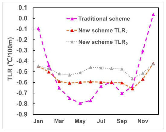
Figure 5.
Comparison of monthly TLRs estimated using the traditional scheme and the new scheme. TLR0 and TLR7 mean the starting buffer used in the new TLR scheme was buffer No. 0 and No. 7, respectively.
3.2. Comparison of Snow Cover Area Simulations
The comparison results of snow cover area simulations driven by the TLRs from the traditional scheme (Base Case) and the new scheme (Case 1) are shown in Figure 6. The results show that there are significant differences in the performance of Base Case and Case 1. Based on the simulation results of the year-to-year monthly snow cover area, the R2 of Base Case (0.42) is lower than that of Case 1 (0.50) (Figure 6a). The performance differences were further enlarged for the simulations of the multiyear-average monthly snow cover area, with the R2 of Base Case and Case 1 as 0.56 and 0.82, respectively (Figure 6b). In general, the accuracy of snow cover area simulation using the new TLR scheme is higher than that using the traditional scheme.
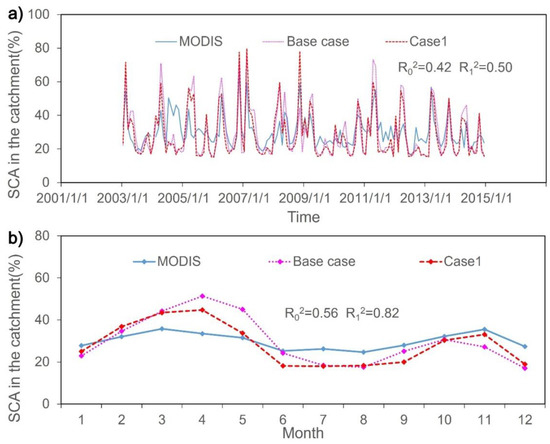
Figure 6.
Comparison of the year-to-year monthly (a) and the multiyear-average monthly (b) snow cover area (SCA) simulated from the J2000 model driven by the TLRs from the traditional scheme (Base Case) and the new scheme (Case 1) during the period of 2003–2014. R02 and R12 are the R-squared values of Base Case and Case 1, respectively.
3.3. Comparison of Runoff Simulations
The comparison results of daily runoff simulations using the traditional TLR scheme (Base Case) and the new TLR scheme (Case 1) are shown in Figure 7. Both cases obtained acceptable accuracy of daily runoff simulations. The performance of Case 1 was better than that of Base Case. The NSEs of Case 1 in the calibration and validation periods were 0.76 and 0.75, which were higher than those of Base Case with NSEs of the two periods of 0.71 and 0.68, respectively. It should be noted that the performance differences between the two TLR schemes were further enlarged in terms of LSE. For the period of validation, the LSE of Base Case was 0.67, which is significantly lower than that of Case 1 (0.81). In addition, the comparison results are generally consistent in terms of NSE, LSR and R2.
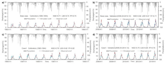
Figure 7.
Comparison of daily runoff simulation results from the J2000 model using the traditional TLR scheme (Base Case, a,b) and the new TLR scheme (Case 1, c,d) for the periods of calibration (a,c) and validation (b,d).
4. Discussion
4.1. The Rationality of the TLRs Estimated Using the New Scheme
Various factors such as solar radiation, humidity (or precipitation) and snow cover were found to have potentially important effects on the spatiotemporal variation of TLR [40,47]. Thus, it is difficult to directly evaluate and compare the seasonal cycles of TLRs estimated from the traditional and new schemes in the case with no observations. The variation range of monthly TLRs estimated from the new scheme is clearly smaller than that from the traditional scheme. The relatively small variation range of monthly TLRs from the new scheme is consistent with He [40], who also found a relatively small seasonal variation of TLRs of the Tibetan Plateau. Previous studies indicated that the monthly TLR of the Tibetan Plateau generally ranges from −0.4 to −0.9 °C/100 m [47,53]. The TLRs estimated using the new scheme are well within these ranges. In contrast, the TLRs estimated using the traditional scheme showed a temperature inversion in December with a positive monthly TLR of 0.04 °C/100 m. Though some studies also observed the phenomena of winter temperature inversion in some regions of China [47], the monthly TLRs of January and December estimated using the traditional scheme are considered abnormal and unreasonable due to the following reasons. The first evidence is that the hydrological simulation using the traditional TLR scheme (i.e., Base Case) produced an abnormal winter peak of runoff, which can be seen in Figure 7 and Figure S1. The much shallower TLR values of winter led to higher air temperatures, further producing much more runoff than the reality, and such abnormal winter peaks did not exist in either the station runoff observations or Case 1. In addition, the winter temperature inversions were mostly reported in Northwestern China [47] or in regions with small elevation variations of the Tibetan Plateau [44], while the standard deviation of elevations for the Karuxung watershed is as high as 413.5 m. Thus, the monthly TLRs estimated by the new scheme are considered more reasonable than the traditional scheme. The abnormal TLR values of winter months estimated by the traditional scheme could be related to the too long distance between the two meteorological stations used.
4.2. Uncertainty and Limitations
Though TLR is a crucial parameter for the hydrological simulation of the Karuxung watershed, other inputs and parameters also have effects on the simulation results. Based on previous studies, the precipitation gradient could be one of the most important factors affecting the results of this study [8,24,54]. Thus, two cases were further tested by replacing the reanalysis-based precipitation gradients of Base Case and Case 1 with the monthly precipitation gradients obtained from the two meteorological stations (i.e., Gyantse and Langkazi) and referred to as Cases 2 and 3, respectively. The runoff simulation results of Cases 2 and 3 are shown in Figure 8. The comparison results of Cases 2 and 3 are consistent with those of Base Case and Case 1 in that the performance in runoff simulation of the case using the new TLR scheme (i.e., Case 3) was better than that of the case using the traditional TLR scheme (i.e., Case 2), e.g., the NSEs of Case 2 for the calibration and validation periods were 0.64 and 0.63, while those of Case 3 were 0.73 and 0.72, respectively. Similar comparison results of Cases 2 and 3 were obtained for snow cover area simulations (Figure 9). Case 3 showed higher R2 of snow cover area than Case 2, and this finding is also consistent with the comparison of snow cover area simulations of Case 1 and Base Case. Thus, even when using different precipitation gradients, the new TLR scheme still improved the simulations of snow cover and runoff. In addition, the finding that Base Case and Case 1 showed better performance in runoff and snow cover simulations than Cases 2 and 3, respectively, indicates that the precipitation gradients derived from the two meteorological stations may be less efficient than those derived from the gridded reanalysis data. This could be due to the low spatial representativeness of the limited number of stations. The uncertainty from precipitation data could also be related to the runoff underestimations of early summer in both Base Case and Case 1. Future studies could collect more reliable precipitation data in the study area to improve the runoff simulations. Previous studies using the J2000 model in different glacierized basins of the Tibetan Platea showed that for runoff simulations, the NSE values were between 0.52 and 0.75, and the R2 values were between 0.56 and 0.91 [17,55]. Considering that the NSE values reported from different cases of this study are all >0.6, with the highest NSE as 0.80 (Table S2), the performance of runoff simulations was considered acceptable.
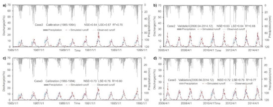
Figure 8.
Comparison of daily runoff simulation results from the J2000 model using the traditional TLR scheme (Case 2, a,b) and the new TLR scheme (Case 3, c,d) for the periods of calibration (a,c) and validation (b,d), when the precipitation gradients were derived from station observations.
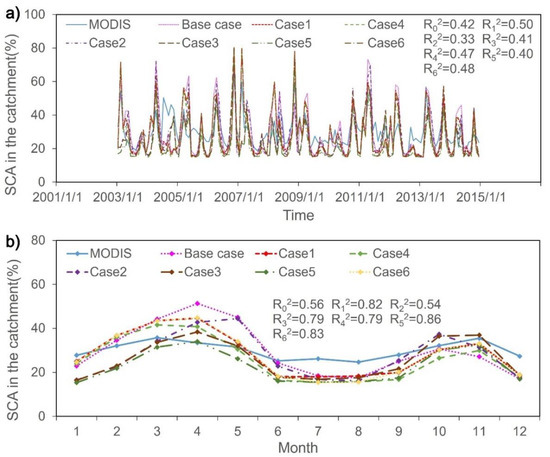
Figure 9.
Comparison of the year-to-year monthly (a) and the multiyear-average monthly (b) snow cover area (SCA) simulated from the seven cases.
The new TLR scheme may also have some inherent uncertainty and limitations. The first uncertainty lies in whether to consider the location of the meteorological station, particularly when the station is outside the watershed. Two additional cases were hence conducted without consideration of the location of the Langkazi station based on Cases 1 and 3 and referred to as Cases 4 and 5, respectively. In other words, the TLR calculation started from the original extent of the Karuxung watershed (rather than the extent of buffers No. 0–7 as mentioned in Section 2.4.2 for both Cases 4 and 5, and the final No. of buffers was also 0 for almost all months. The runoff simulation results of Cases 4 and 5 are shown in Figure 10. Cases 4 and 5 showed poorer performance in runoff simulations (i.e., with lower NSE, LSE and R2) than Cases 1 and 3, respectively. Though Case 5 showed higher R2 of multiyear-average monthly snow cover area than Case 3 and even Case 1 (Figure 9), the new TLR scheme considering the location of the Langkazi station generally outperformed it in the hydrological simulations of Karuxung. This could be related to the different spatial representativeness. As shown in Figure 11, the compositions of land cover types were very different between buffer No. 0 and the area that extends to buffer No. 7, with the former’s major land cover type as barren (about 55%) and the latter’s major land cover type as grasslands (about 62%). Thus, future studies may further improve the TLR scheme by considering the potentially important effects of land cover types. Another limitation of this study could be that the new TLR scheme failed to produce TLRs for July and August when there were not enough valid LST pixels. Though a temporally linear interpolation was employed here to obtain TLRs of July and August, another possible solution could be using the gap-filled LST data. To provide a parametrization scheme entirely based on remote sensing, a global gap-filled daily LST dataset was further tested and used to estimate the TLRs of the two months following the same algorithm as the new TLR scheme. The gap-filled LST data were recently developed using a novel spatiotemporal interpolation method, and the root-mean-square error of the cross-validation for nighttime LST is reported to be less than 1.4 K [56]. An additional case was hence conducted by replacing the linearly interpolated TLRs of July and August in Case 1 with those produced using the gap-filled LST data, referred to as “Case 6”. The simulation results of SCA and runoff from Case 6 were compared with those from Base Case as shown in Figures S2 and S3. In general, Case 6 showed better accuracy than Base Case in both SCA and runoff (Table S2) indicating that the new TLR scheme still performed better than the station based on the gap-filled LST data being used for July and August. However, the runoff simulation accuracy of Case 6 was notably lower than that of Case 1. This is mainly because the TLRs of July and August of Case 6 are −0.44 and −0.46 °C/100 m and significantly shallower than those of Case 1 (Figure 5). The reduced accuracy of Case 6 compared with Case 1 implies that the gap-filled LST data used for estimating TLRs of July and August could be further improved in future.
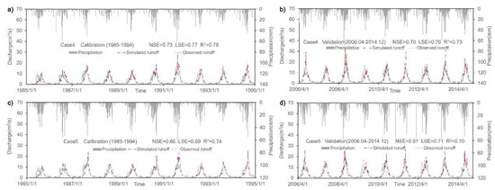
Figure 10.
Comparison of daily runoff simulation results from the J2000 model using the traditional TLR scheme (Case 4, a,b) and the new TLR scheme (Case 5, c,d) for the periods of calibration (a,c) and validation (b,d), when the precipitation gradients were derived from station observations.
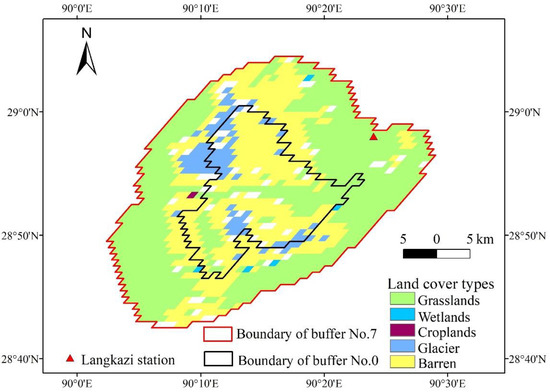
Figure 11.
Comparison of distributions of land cover types between the extent of buffer No. 0 and that of buffers 0–7.
The problem of high cloud cover may also be related to the significant underestimation of snow cover simulation in July and August of Case 1 (Figure 6). It should be noted that the remote sensing snow cover product used as ground truth may also have large uncertainty in July and August when the cloud cover is very high. To better evaluate the new TLR scheme, both Base Case and Case 1 were reconducted by removing the months of July and August. The results are shown in Figure S4. The R2 of monthly snow cover area was increased modestly for both cases, and Case 1 still showed better accuracy than Base Case. It should also be noted that various methods have been developed for removing the cloud-contaminated data of MODIS snow cover products [57]. For example, Muhammad [58] developed a novel cloud-free snow cover dataset by combing MODIS snow cover data and the glacier data from Randolph Glacier Inventory 6.0 with better accuracy than the original MODIS data. Thus, future studies could use more kinds of cloud-free snow cover data for reducing the uncertainty related to the selection of snow cover products.
The accuracy of snow cover area and runoff simulations of all cases is summarized in Table S2. In general, Case 1 that uses both the new TLR scheme and the reanalysis-based precipitation gradients showed the best performance in almost all the evaluation metrics except the R2 of multiyear-average monthly snow cover area. Another limitation of this study is that the machine learning models, which are also important and efficient tools for forecasting changes of snow cover and discharge, were not employed here, e.g., the long short-term memory (LSTM) model was used to forecast the temporal changes of snow cover in a mountainous region in the Northwestern Himalayas and achieved a good performance [39]. Future studies can further evaluate the performance of the TLR scheme here developed in applications of machine learning methods and compare the performance of different kinds of models. In addition, the computational complexity is an important factor that should be considered for constructing models to forecast environmental changes [59,60]. One model run takes about 1.5 minutes to simulate discharge of the whole period using the J2000 model, and future studies can further improve the computational efficiency of hydrological simulations using the J2000 model. Despite five cases that were additionally conducted to test the effects of precipitation and the inherent setting of the new TLR scheme, we acknowledge that there are more uncertainty sources that were not addressed in this study. However, a complete and comprehensive uncertainty analysis that considers all the potential factors was impractical for a process-based hydrological model with various inputs and parameters due to a high computing burden. The new TLR scheme can be further evaluated in more watersheds with scarce data or by considering more uncertainty sources in future.
4.3. Implication of the New TLR Scheme for Snow Cover and Runoff Simulations and Comparison with Existing Studies
Though MODIS LST data have been used to estimate monthly TLR for application in hydrological simulations, there are obvious differences between those studies and the present work [43,61]. Firstly, previous studies were conducted in the Upper Yellow River Basin (UYRB) with no glaciers. The contribution of snowmelt to total runoff of the UYRB is less than 25% [6]; however, the contribution of meltwater including snowmelt and glacier-melt to the total runoff of the Karuxung watershed was > 65% in all the six cases (Figure 12). The contrasting contributions of meltwater led to different importance of TLR in runoff simulations. Secondly, the validation methods of snow cover simulations were different. Previous studies mainly used microwave-based snow depth product with a coarse resolution (0.25°) as reference data [43,61], which is not suitable for meso- and micro-scale watersheds. Due to the high spatial resolution of about 500m, MODIS-based snow cover data can capture snow cover dynamics of the watershed more accurately and may thus be taken as more efficient reference data for evaluating snow cover simulations. For the first time, this study demonstrated that the new TLR scheme based on MODIS LST improved simulations of snow cover area (Figure 6 and Figure 9). Last but not least, the new TLR scheme proposed here considers the effects of missing data caused by cloud contamination and the location of the meteorological station, leading to an increased applicability for meso- and micro-scale watersheds with scarce observations.

Figure 12.
Comparison of runoff components during the calibration (a) and validation (b) periods for the seven cases.
In addition, due to the relatively small contribution of meltwater to the total runoff of the UYRB, the improvement in runoff simulation by using remote sensing TLR seems to be minimal in previous study [43]. In contrast, new implications of the proposed TLR scheme based on remote sensing for runoff simulations were obtained in this study. This study indicated that the new TLR scheme significantly improved the runoff simulations in months with relatively low discharge (i.e., November–May, according to the monthly runoff shown in Figure S5), compared with the traditional scheme based on station observations. An important example of evidence is that the LSE of Case 1 is significantly higher than that of Base Case. The definition of LSE assigns a heavier weight to low runoff values and is more concerned with the accuracy of simulation of low-runoff months compared with NSE and R2. The correlation analysis (Figure S6) further supports this finding. The correlation coefficients of runoff in low-runoff months were 0.56 and 0.54 for the calibration and validation periods in Case 1, which were significantly higher than those in Base Case as 0.31 and 0.14, respectively. Another notable improvement in runoff simulations by the new TLR scheme is that the erroneous winter runoff peak in Base Case disappeared in Case 1 (see Figure S1). Though low-runoff months seem to be less important than summer months in terms of the magnitude of discharge, the meltwater in low-runoff months could be important for agricultural production in the downstream regions, e.g., Qin [62] found that spring snowmelts are crucial for meeting the water demands of wheat growth in middle-high latitude regions of the Northern Hemisphere. In this case, if the snow that accumulates in winter melts earlier than the reality (e.g., resulting in erroneous simulations of winter discharge peak as in Base Case), the meltwater in spring could be underestimated, which could further impact analysis related to agricultural water management.
5. Conclusions
This study developed a new parameterization scheme of temperature lapse rate (TLR) for the hydrological simulation of the glacierized Karuxung River Basin based on MODIS LST. For the first time, a remote-sensing-based TLR scheme that is basin-oriented in consideration of the location of meteorological stations and the missing data caused by cloud contamination was proposed and tested in a typical glacierized watershed. The evaluation results indicated that in the Karuxung watershed, the TLRs estimated from the new scheme have a more reasonable seasonal pattern than the traditional scheme that relied on a limited number of meteorological stations. The new TLR scheme was demonstrated to improve simulations of the monthly snow cover area and the discharge of low-runoff months, possibly due to its clearly larger spatial representativeness of temperature changes across the Karuxung watershed.
This study implies that when estimating TLR in an alpine basin with scarce observations, the traditional scheme based on a limited number of stations may be unreliable and could result in large errors of snow cover and runoff simulations. In this case, the TLR scheme based on remote sensing LST could be a better alternative. Furthermore, this study indicates that when interpolating air temperatures using the remote sensing TLR, the location of the meteorological station needs to be considered. Future efforts should be made to further reduce the adverse effects of high cloud cover on remote sensing TLR and consider the potentially important effects of land cover types and precipitation inputs [63]. Considering that the machine learning models are also important tools for forecasting snow cover and discharge changes, the performance of the new TLR scheme should be further evaluated in applications using machine learning models in future. The new TLR scheme proposed here is not limited to the Karuxung River Basin and can be easily applied to other alpine watersheds globally.
Supplementary Materials
The following supporting information can be downloaded at: https://www.mdpi.com/article/10.3390/rs14194973/s1, Table S1: Other calibration parameters in the J2000 hydrological model; Table S2: Runoff and SCA simulation accuracy of all cases; Figure S1: Comparison of daily runoff simulation results from the J2000 model using the traditional TLR scheme (Base Case) and the new TLR scheme (Case 1) for the periods of validation; Figure S2: Comparison of monthly snow cover area (SCA) simulations between Base Case and Case 6; Figure S3: Comparison of daily runoff simulation results between Base Case and Case 6; Figure S4: Comparison of monthly snow cover area (SCA) simulations between Base Case and Case 1 without consideration of July and August; Figure S5: Multiyear-average monthly total runoff; Figure S6: Comparison of correlation analysis of daily simulation runoff and observation runoff (November–May) results from the J2000 model using the traditional TLR scheme (a and b) and the new TLR scheme (c and d) for the periods of calibration (a and c) and validation (b and d).
Author Contributions
Conceptualization, H.Z.; methodology, W.S. and H.T.; software, W.S.; formal analysis, W.S.; resources, H.Z., X.S. and X.M.; supervision, H.Z., H.T. and Y.X.; writing—original draft preparation, W.S.; writing—review and editing, H.Z.; funding acquisition, H.Z. and X.S. All authors have read and agreed to the published version of the manuscript.
Funding
This study is supported by the National Natural Science Foundation of China (41701079), and the project ZR2021MD029 supported by Shandong Provincial Natural Science Foundation.
Data Availability Statement
Not applicable.
Acknowledgments
We acknowledge Fan Zhang for the data support.
Conflicts of Interest
The authors declare no conflict of interest.
References
- Viviroli, D.; Dürr, H.H.; Messerli, B.; Meybeck, M.; Weingartner, R. Mountains of the world, water towers for humanity: Typology, mapping, and global significance. Water Resour. Res. 2007, 43, W07447. [Google Scholar] [CrossRef]
- Immerzeel, W.W.; van Beek, L.P.; Bierkens, M.F. Climate change will affect the Asian water towers. Science 2010, 328, 1382–1385. [Google Scholar] [CrossRef] [PubMed]
- Yao, T.; Bolch, T.; Chen, D.; Gao, J.; Immerzeel, W.; Piao, S.; Su, F.; Thompson, L.; Wada, Y.; Wang, L.; et al. The imbalance of the Asian water tower. Nat. Rev. Earth Environ. 2022, 3, 618–632. [Google Scholar] [CrossRef]
- Yu, M.; Chen, X.; Li, L.; Bao, A.; de la Paix, M.J. Incorporating accumulated temperature and algorithm of snow cover calculation into the snowmelt runoff model. Hydrol. Processes 2013, 27, 3589–3595. [Google Scholar] [CrossRef]
- Lutz, A.F.; Immerzeel, W.W.; Shrestha, A.B.; Bierkens, M.F.P. Consistent increase in High Asia’s runoff due to increasing glacier melt and precipitation. Nat. Clim. Chang. 2014, 4, 587–592. [Google Scholar] [CrossRef]
- Zhang, L.; Su, F.; Yang, D.; Hao, Z.; Tong, K. Discharge regime and simulation for the upstream of major rivers over Tibetan Plateau. J. Geophys. Res. Atmos. 2013, 118, 8500–8518. [Google Scholar] [CrossRef]
- Kiani, R.S.; Ali, S.; Ashfaq, M.; Khan, F.; Muhammad, S.; Reboita, M.S.; Farooqi, A. Hydrological projections over the Upper Indus Basin at 1.5 degrees C and 2.0 degrees C temperature increase. Sci. Total Environ. 2021, 788, 147759. [Google Scholar] [CrossRef] [PubMed]
- Zhang, F.; Zhang, H.; Hagen, S.C.; Ye, M.; Wang, D.; Gui, D.; Zeng, C.; Tian, L.; Liu, J. Snow cover and runoff modelling in a high mountain catchment with scarce data: Effects of temperature and precipitation parameters. Hydrol. Processes 2015, 29, 52–65. [Google Scholar] [CrossRef]
- Viviroli, D.; Archer, D.R.; Buytaert, W.; Fowler, H.J.; Greenwood, G.B.; Hamlet, A.F.; Huang, Y.; Koboltschnig, G.; Litaor, M.I.; López-Moreno, J.I.; et al. Climate change and mountain water resources: Overview and recommendations for research, management and policy. Hydrol. Earth Syst. Sci. 2011, 15, 471–504. [Google Scholar] [CrossRef]
- Hock, R. Temperature index melt modelling in mountain areas. J. Hydrol. 2003, 282, 104–115. [Google Scholar] [CrossRef]
- Kraaijenbrink, P.D.A.; Stigter, E.E.; Yao, T.; Immerzeel, W.W. Climate change decisive for Asia’s snow meltwater supply. Nat. Clim. Chang. 2021, 11, 591–597. [Google Scholar] [CrossRef]
- Ding, B.H.; Yang, K.; Yang, W.; He, X.B.; Chen, Y.Y.; Lazhu; Guo, X.F.; Wang, L.; Wu, H.; Yao, T.D. Development of a Water and Enthalpy Budget-based Glacier mass balance Model (WEB-GM) and its preliminary validation. Water Resour. Res. 2017, 53, 3146–3178. [Google Scholar] [CrossRef]
- Naz, B.S.; Frans, C.D.; Clarke, G.K.C.; Burns, P.; Lettenmaier, D.P. Modeling the effect of glacier recession on streamflow response using a coupled glacio-hydrological model. Hydrol. Earth Syst. Sci. 2014, 18, 787–802. [Google Scholar] [CrossRef]
- Shrestha, M.; Koike, T.; Hirabayashi, Y.; Xue, Y.K.; Wang, L.; Rasul, G.; Ahmad, B. Integrated simulation of snow and glacier melt in water and energy balance-based, distributed hydrological modeling framework at Hunza River Basin of Pakistan Karakoram region. J. Geophys. Res.-Atmos. 2015, 120, 4889–4919. [Google Scholar] [CrossRef]
- Huang, N.; Shi, G. The significance of vertical moisture diffusion on drifting snow sublimation near snow surface. Cryosphere 2017, 11, 3011–3021. [Google Scholar] [CrossRef]
- Xie, Z.P.; Hu, Z.Y.; Ma, Y.M.; Sun, G.H.; Gu, L.L.; Liu, S.; Wang, Y.D.; Zheng, H.X.; Ma, W.Q. Modeling Blowing Snow Over the Tibetan Plateau With the Community Land Model: Method and Preliminary Evaluation. J. Geophys. Res.-Atmos. 2019, 124, 9332–9355. [Google Scholar] [CrossRef]
- Gao, T.G.; Kang, S.C.; Lan, C.; Zhang, T.J.; Guoshuai, Z.S.; Yulan, Z.L.; Sillanpaa, M. Simulation and analysis of glacier runoff and mass balance in the Nam Co basin, southern Tibetan Plateau. J. Glaciol. 2015, 61, 447–460. [Google Scholar] [CrossRef]
- Steudel, T.; Bugan, R.; Kipka, H.; Pfennig, B.; Fink, M.; de Clercq, W.; Flugel, W.A.; Helmschrot, J. Implementing contour bank farming practices into the J2000 model to improve hydrological and erosion modelling in semi-arid Western Cape Province of South Africa. Hydrol. Res. 2015, 46, 192–211. [Google Scholar] [CrossRef][Green Version]
- Martinec, J. Subsurface flow from snowmelt traced by tritium. Water Resour. Res. 1975, 11, 496–498. [Google Scholar] [CrossRef]
- Terink, W.; Lutz, A.F.; Simons, G.W.H.; Immerzeel, W.W.; Droogers, P. SPHY v2.0: Spatial Processes in HY drology. Geosci. Model Dev. 2015, 8, 2009–2034. [Google Scholar] [CrossRef]
- Yang, Y.; Chen, R.; Liu, G.; Liu, Z.; Wang, X. Trends and variability in snowmelt in China under climate change. Hydrol. Earth Syst. Sci. 2022, 26, 305–329. [Google Scholar] [CrossRef]
- Zhang, H.; Zhang, F.; Che, T.; Yan, W.; Ye, M. Investigating the ability of multiple reanalysis datasets to simulate snow depth variability over mainland China from 1981 to 2018. J. Clim. 2021, 34, 9957–9972. [Google Scholar] [CrossRef]
- Zhang, H.; Zhang, F.; Zhang, G.; Yan, W. Why Do CMIP6 Models Fail to Simulate Snow Depth in Terms of Temporal Change and High Mountain Snow of China Skillfully? Geophys. Res. Lett. 2022, 49, e2022GL098888. [Google Scholar] [CrossRef]
- Immerzeel, W.W.; Petersen, L.; Ragettli, S.; Pellicciotti, F. The importance of observed gradients of air temperature and precipitation for modeling runoff from a glacierized watershed in the Nepalese Himalayas. Water Resour. Res. 2014, 50, 2212–2226. [Google Scholar] [CrossRef]
- Petersen, L.; Pellicciotti, F. Spatial and temporal variability of air temperature on a melting glacier: Atmospheric controls, extrapolation methods and their effect on melt modeling, Juncal Norte Glacier, Chile. J. Geophys. Res.-Atmos. 2011, 116, 23. [Google Scholar] [CrossRef]
- Kirchner, M.; Faus-Kessler, T.; Jakobi, G.; Leuchner, M.; Ries, L.; Scheel, H.E.; Suppan, P. Altitudinal temperature lapse rates in an Alpine valley: Trends and the influence of season and weather patterns. Int. J. Climatol. 2013, 33, 539–555. [Google Scholar] [CrossRef]
- Luo, Y.; Arnold, J.; Liu, S.Y.; Wang, X.Y.; Chen, X. Inclusion of glacier processes for distributed hydrological modeling at basin scale with application to a watershed in Tianshan Mountains, northwest China. J. Hydrol. 2013, 477, 72–85. [Google Scholar] [CrossRef]
- Sun, R.; Zhang, X.Q.; Sun, Y.; Zheng, D.; Fraedrich, K. SWAT-Based Streamflow Estimation and Its Responses to Climate Change in the Kadongjia River Watershed, Southern Tibet. J. Hydrometeorol. 2013, 14, 1571–1586. [Google Scholar] [CrossRef]
- Hao, Z.; Zhang, Y.; Yang, C.; Li, J.; Dawa, T. Effects of topography and snowmelt on hydrologic simulation in the Yellow River’s source region. Adv. Water Sci. 2013, 24, 311–318. [Google Scholar]
- Immerzeel, W.W.; van Beek, L.P.H.; Konz, M.; Shrestha, A.B.; Bierkens, M.F.P. Hydrological response to climate change in a glacierized catchment in the Himalayas. Clim. Chang. 2012, 110, 721–736. [Google Scholar] [CrossRef] [PubMed]
- Michlmayr, G.; Lehning, M.; Koboltschnig, G.; Holzmann, H.; Zappa, M.; Mott, R.; Schoner, W. Application of the Alpine 3D model for glacier mass balance and glacier runoff studies at Goldbergkees, Austria. Hydrol. Processes 2008, 22, 3941–3949. [Google Scholar] [CrossRef]
- Navarro-Serrano, F.; Lopez-Moreno, J.I.; Azorin-Molina, C.; Alonso-Gonzalez, E.; Tomas-Burguera, M.; Sanmiguel-Vallelado, A.; Revuelto, J.; Vicente-Serrano, S.M. Estimation of near-surface air temperature lapse rates over continental Spain and its mountain areas. Int. J. Climatol. 2018, 38, 3233–3249. [Google Scholar] [CrossRef]
- Rao, Y.; Liang, S.; Wang, D.; Yu, Y.; Song, Z.; Zhou, Y.; Shen, M.; Xu, B. Estimating daily average surface air temperature using satellite land surface temperature and top-of-atmosphere radiation products over the Tibetan Plateau. Remote Sens. Environ. 2019, 234, 111462. [Google Scholar] [CrossRef]
- Xu, Y.; Knudby, A.; Shen, Y.; Liu, Y. Mapping monthly air temperature in the Tibetan Plateau from MODIS data based on machine learning methods. IEEE J. Sel. Top. Appl. Earth Obs. Remote Sens. 2018, 11, 345–354. [Google Scholar] [CrossRef]
- Vanhellemont, Q. Combined land surface emissivity and temperature estimation from Landsat 8 OLI and TIRS. ISPRS J. Photogramm. Remote Sens. 2020, 166, 390–402. [Google Scholar] [CrossRef]
- Shen, H.; Jiang, Y.; Li, T.; Cheng, Q.; Zeng, C.; Zhang, L. Deep learning-based air temperature mapping by fusing remote sensing, station, simulation and socioeconomic data. Remote Sens. Environ. 2020, 240, 111692. [Google Scholar] [CrossRef]
- Haq, M.A.; Baral, P.; Yaragal, S.; Pradhan, B. Bulk Processing of Multi-Temporal Modis Data, Statistical Analyses and Machine Learning Algorithms to Understand Climate Variables in the Indian Himalayan Region. Sensors 2021, 21, 7416. [Google Scholar] [CrossRef] [PubMed]
- Haq, M.A.; Baral, P.; Yaragal, S.; Rahaman, G. Assessment of trends of land surface vegetation distribution, snow cover and temperature over entire Himachal Pradesh using MODIS datasets. Nat. Resour. Modeling 2020, 33, e12262. [Google Scholar] [CrossRef]
- Haq, M.A.; Ahmed, A.; Khan, I.; Gyani, J.; Mohamed, A.; Attia, E.A.; Mangan, P.; Pandi, D. Analysis of environmental factors using AI and ML methods. Sci. Rep. 2022, 12, 13267. [Google Scholar] [CrossRef]
- He, Y.; Wang, K. Contrast patterns and trends of lapse rates calculated from near-surface air and land surface temperatures in China from 1961 to 2014. Sci. Bull. 2020, 65, 1217–1224. [Google Scholar] [CrossRef]
- Firozjaei, M.K.; Fathololoumi, S.; Alavipanah, S.K.; Kiavarz, M.; Vaezi, A.R.; Biswas, A. A new approach for modeling near surface temperature lapse rate based on normalized land surface temperature data. Remote Sens. Environ. 2020, 242, 111746. [Google Scholar] [CrossRef]
- Zhang, H.; Zhang, F.; Zhang, G.; Che, T.; Yan, W. How Accurately Can the Air Temperature Lapse Rate Over the Tibetan Plateau Be Estimated From MODIS LSTs? J. Geophys. Res. Atmos. 2018, 123, 3943–3960. [Google Scholar] [CrossRef]
- Wang, L.; Sun, L.; Shrestha, M.; Li, X.; Liu, W.; Zhou, J.; Yang, K.; Lu, H.; Chen, D. Improving snow process modeling with satellite-based estimation of near-surface-air-temperature lapse rate. J. Geophys. Res. Atmos. 2016, 121, 12005–12030. [Google Scholar] [CrossRef]
- Zhang, H.B.; Immerzeel, W.W.; Zhang, F.; de Kok, R.J.; Gorrie, S.J.; Ye, M. Creating 1-km long-term (1980–2014) daily average air temperatures over the Tibetan Plateau by integrating eight types of reanalysis and land data assimilation products downscaled with MODIS-estimated temperature lapse rates based on machine learning. Int. J. Appl. Earth Obs. Geoinf. 2021, 97, 102295. [Google Scholar] [CrossRef]
- Wang, Y.; Wang, L.; Li, X.; Chen, D. Temporal and spatial changes in estimated near-surface air temperature lapse rates on Tibetan Plateau. Int. J. Climatol. 2018, 38, 2907–2921. [Google Scholar] [CrossRef]
- Hao, X.H.; Luo, S.Q.; Che, T.; Wang, J.; Li, H.Y.; Dai, L.Y.; Huang, X.D.; Feng, Q.S. Accuracy assessment of four cloud-free snow cover products over the Qinghai-Tibetan Plateau. Int. J. Digit. Earth 2019, 12, 375–393. [Google Scholar] [CrossRef]
- Li, X.; Wang, L.; Chen, D.; Yang, K.; Xue, B.; Sun, L. Near-surface air temperature lapse rates in the mainland China during 1962–2011. J. Geophys. Res. Atmos. 2013, 118, 7505–7515. [Google Scholar] [CrossRef]
- Nepal, S. Evaluating Upstream Downstream Linkages of Hydrological Dynamics in the Himalayan Region. Ph.D. Thesis, Friedrich-Schiller-Universität Jena, Jena, Germany, 2012. [Google Scholar]
- Krause, P. Quantifying the impact of land use changes on the water balance of large catchments using the J2000 model. Phys. Chem. Earth 2002, 27, 663–673. [Google Scholar] [CrossRef]
- Maussion, F.; Scherer, D.; Mölg, T.; Collier, E.; Curio, J.; Finkelnburg, R. Precipitation Seasonality and Variability over the Tibetan Plateau as Resolved by the High Asia Reanalysis. J. Clim. 2014, 27, 1910–1927. [Google Scholar] [CrossRef]
- Hock, R. A distributed temperature-index ice- and snowmelt model including potential direct solar radiation. J. Glaciol. 1999, 45, 101–111. [Google Scholar] [CrossRef]
- Hotovy, O.; Jenicek, M. The impact of changing subcanopy radiation on snowmelt in a disturbed coniferous forest. Hydrol. Processes 2020, 34, 5298–5314. [Google Scholar] [CrossRef]
- Gao, L.; Bernhardt, M.; Schulz, K.; Chen, X.W. Elevation correction of ERA-Interim temperature data in the Tibetan Plateau. Int. J. Climatol. 2017, 37, 3540–3552. [Google Scholar] [CrossRef]
- Wang, L.; Zhang, F.; Zhang, H.; Scott, C.A.; Zeng, C.; Shi, X. Intensive precipitation observation greatly improves hydrological modelling of the poorly gauged high mountain Mabengnong catchment in the Tibetan Plateau. J. Hydrol. 2018, 556, 500–509. [Google Scholar] [CrossRef]
- Gao, T.G.; Kang, S.C.; Krause, P.; Cuo, L.; Nepal, S. A test of J2000 model in a glacierized catchment in the central Tibetan Plateau. Environ. Earth Sci. 2012, 65, 1651–1659. [Google Scholar] [CrossRef]
- Zhang, T.; Zhou, Y.Y.; Zhu, Z.Y.; Li, X.M.; Asrar, G.R. A global seamless 1 km resolution daily land surface temperature dataset (2003–2020). Earth Syst. Sci. Data 2022, 14, 651–664. [Google Scholar] [CrossRef]
- Li, X.H.; Jing, Y.H.; Shen, H.F.; Zhang, L.P. The recent developments in cloud removal approaches of MODIS snow cover product. Hydrol. Earth Syst. Sci. 2019, 23, 2401–2416. [Google Scholar] [CrossRef]
- Muhammad, S.; Thapa, A. Daily Terra-Aqua MODIS cloud-free snow and Randolph Glacier Inventory 6.0 combined product (M*D10A1GL06) for high-mountain Asia between 2002 and 2019. Earth Syst. Sci. Data 2021, 13, 767–776. [Google Scholar] [CrossRef]
- Haq, M.A. SMOTEDNN: A Novel Model for Air Pollution Forecasting and AQI Classification. CMC—Comput. Mater. Contin. 2022, 71, 1403–1425. [Google Scholar] [CrossRef]
- Haq, M.A. CDLSTM: A Novel Model for Climate Change Forecasting. CMC—Comput. Mater. Contin. 2022, 71, 2363–2381. [Google Scholar] [CrossRef]
- Liu, W.B.; Wang, L.; Sun, F.B.; Li, Z.H.; Wang, H.; Liu, J.H.; Yang, T.; Zhou, J.; Qi, J. Snow Hydrology in the Upper Yellow River Basin Under Climate Change: A Land Surface Modeling Perspective. J. Geophys. Res.-Atmos. 2018, 123, 12676–12691. [Google Scholar] [CrossRef]
- Qin, Y.; Abatzoglou, J.T.; Siebert, S.; Huning, L.S.; AghaKouchak, A.; Mankin, J.S.; Hong, C.P.; Tong, D.; Davis, S.J.; Mueller, N.D. Agricultural risks from changing snowmelt. Nat. Clim. Chang. 2020, 10, 459–465. [Google Scholar] [CrossRef]
- Ma, N.; Zhang, Y. Increasing Tibetan Plateau terrestrial evapotranspiration primarily driven by precipitation. Agric. For. Meteorol. 2020, 317, 108887. [Google Scholar] [CrossRef]
Publisher’s Note: MDPI stays neutral with regard to jurisdictional claims in published maps and institutional affiliations. |
© 2022 by the authors. Licensee MDPI, Basel, Switzerland. This article is an open access article distributed under the terms and conditions of the Creative Commons Attribution (CC BY) license (https://creativecommons.org/licenses/by/4.0/).