Article

Tree Detection and Species Classification in a Mixed Species Forest Using Unoccupied Aircraft System (UAS) RGB and Multispectral Imagery

School of Geography, Planning, and Spatial Sciences, University of Tasmania, Sandy Bay, TAS 7005, Australia
*
Author to whom correspondence should be addressed.
Remote Sens. 2022, 14(19), 4963; https://doi.org/10.3390/rs14194963
Submission received: 12 August 2022 / Revised: 23 September 2022 / Accepted: 29 September 2022 / Published: 5 October 2022
(This article belongs to the Section Ecological Remote Sensing)

Abstract

:
Information on tree species and changes in forest composition is necessary to understand species-specific responses to change, and to develop conservation strategies. Remote sensing methods have been increasingly used for tree detection and species classification. In mixed species forests, conventional tree detection methods developed with assumptions about uniform tree canopy structure often fail. The main aim of this study is to identify effective methods for tree delineation and species classification in an Australian native forest. Tree canopies were delineated at three different spatial scales of analysis: (i) superpixels representing small elements in the tree canopy, (ii) tree canopy objects generated using a conventional segmentation technique, multiresolution segmentation (MRS), and (iii) individual tree bounding boxes detected using deep learning based on the DeepForest open-source algorithm. Combinations of spectral, texture, and structural measures were tested to assess features relevant for species classification using RandomForest. The highest overall classification accuracies were achieved at the superpixel scale (0.84 with all classes and 0.93 with Eucalyptus classes grouped). The highest accuracies at the individual tree bounding box and object scales were similar (0.77 with Eucalyptus classes grouped), highlighting the potential of tree detection using DeepForest, which uses only RGB, compared to site-specific tuning with MRS using additional layers. This study demonstrates the broad applicability of DeepForest and superpixel approaches for tree delineation and species classification. These methods have the potential to offer transferable solutions that can be applied in other forests.

1. Introduction

Drought-induced declines and tree mortality have been reported in forests across Australia [1,2,3]. Monitoring shifts in forest composition due to species-specific susceptibility to extreme events requires high-resolution tree species maps. These maps can help to understand the ecology of species, functioning of forests and their response to change, and effectively set conservation priorities [4]. Field studies on species distribution are sparse, and this information can be time-consuming and difficult to collect solely through field assessment and monitoring [2]. Tree species classification studies based on remote sensing in Australian mixed species forests are limited. Eucalyptus species dominate most forest and woodland landscapes in Australia [5]. Diversity in species, age, and canopy structure in Eucalyptus-dominant forests make it challenging to apply many of the commonly used algorithms for tree delineation. In addition, their overlapping and open canopy structure, pendulous leaves, spectral similarity between species, and variability within a single species due to different growth stages and due to gaps in the canopy make it difficult to classify Eucalyptus species [6,7]. However, there is a need to investigate methods that are effective in mapping tree species in these forests as they occur in large areas on the Australian continent. Studies have used airborne hyperspectral imagery for species classification in Australian mixed species forests [6,7,8,9,10]. Unoccupied aircraft systems (UASs also known as UAVs or drones) provide an intermediate scale to monitor biodiversity and enable upscaling from field-based measurements to landscape level estimation [11]. UASs are well suited to capture data at a fine spatial resolution and enable timely assessments to measure species response to change.
The classification of tree species using fine spatial resolution imagery is challenging as individual pixels cover different components of the tree. The spectral signature of a single species comprising its wide range of structural elements, such as leaves, branches, stem, and bark, is hard to define [12]. As tree crowns are much larger than the pixel size, Object Based Image Analysis (OBIA) using individual tree canopies is often deemed more appropriate than pixel-level classification [13]. Tree species classification therefore relies on grouping pixels into tree canopy objects using tree detection and tree-crown delineation [14]. Tree detection algorithms have been used to locate treetops and applied successfully in coniferous forests with even-aged trees and uniform structure [14,15,16]. UASs have been increasingly used for monitoring in natural coniferous forests [17,18] and plantations [19], but studies in natural, mixed species forests are limited [20,21]. Conventional individual tree crown delineation algorithms make assumptions about uniformity of tree crowns in size and shape, and clear boundaries between crowns [22]. Tree detection is challenging in mixed species and multi-layered forests as these assumptions often fail [4]. In mixed species forests, image segmentation methods have been used with extensive parameter tuning to generate tree canopy objects for classification [21,23,24]. The identification of settings that worked across a diverse site with varying canopy sizes is an iterative, time-consuming process that requires visual assessment, expert knowledge, and species-specific fine-tuning [4,21]. Furthermore, solutions that achieve acceptable levels of classification accuracy in one forest may not work in another and, hence, are site-specific.
Superpixel segmentation is a recently applied technique that overcomes the challenge of parameter-tuning in pixel-based segmentation. While the aim in conventional segmentation methods in OBIA is to create tree canopy objects, superpixels are an intermediate scale between pixels and meaningful real-world objects [25]. This can be used to generate similar sized objects that adhere to image boundaries without time-consuming parameter tuning. To date, the technique has been applied in urban forests [26], orchards [27], and for land cover classification [28], but it has not been used for tree species classification in natural forests.
Machine learning classifiers are mostly used for tree species classification with UAS data [18,20,29]. RandomForest [30] is popular in remotely sensed image classification as it can be used to estimate the importance of different features in addition to its excellent performance in many studies [18,20,21,31]. Relevant features were found to differ with several factors including the scale of analysis, forest type, separability of tree species, and variability within the study site [20,21].
Recently, the deep learning (DL) method of convolutional neural networks (CNNs) has been applied for vegetation remote sensing [32]. The advantage with CNN is that the parameter tuning with image segmentation and feature selection with machine learning classifiers is unnecessary as the CNN model learns important features from the raw data through an iterative training process. While DL can be used to both detect and classify objects, the use of these methods in the context of vegetation remote sensing is very new and challenging in natural forests [32]. DL-based tree detection using UAS data has been limited to detecting trees of a single species [33,34]. The availability of CNN implementations in DL libraries has facilitated their use in tree species classification in natural coniferous sites [35], urban forests [36] and plantations [37]. Most tree species classification studies still delineate tree canopies manually [38] or use conventional segmentation algorithms [39], and therefore challenges in mixed species forests remain. DL models when trained and validated on extensive reference datasets have the potential to offer a transferable solution to tree detection and species classification across different forests. However, CNNs require a large amount of training data from which connections can be learnt. Several techniques can be used to compensate for small reference datasets. Transfer learning is a technique used to both increase the amount of training data and to speed up training [32,39,40]. There are various transfer learning approaches that Kattenborn et al. [32] classified into two main strategies: (i) The shallow strategy where models are pre-trained on large, open access image databases. These databases, such as ImageNet, contain generic images (often not remotely sensed images or images of the target class) that are used by the CNN to learn lower-level patterns. Only the last layers of the CNN are fine-tuned for higher level and task-specific features using images specific to the research problem. (ii) The deep strategy where the entire network is re-trained using a given dataset [40]. A promising new development in applying deep learning for tree detection is the release of DeepForest, an open-source Python package for delineating trees [41]. DeepForest includes a CNN model that was developed and trained using airborne RGB and lidar data from 22 National Ecological Observatory Network (NEON) sites using an unsupervised lidar-based algorithm and manual annotations of RGB imagery. The pre-built DeepForest model supports the second transfer learning strategy mentioned above, where the entire model is re-trained with an additional dataset. Hence, this open-source model can potentially be used for individual tree detection using RGB imagery and re-trained for different forest types using additional training data from the study site.
The overarching aim of this study is to identify effective methods for tree delineation and species classification from ultrahigh-resolution UAS data of a mixed, dry sclerophyll forest in Australia. The specific objectives are to:
  • Establish whether individual tree detection based on deep learning can achieve better classification accuracies compared to canopy delineation through MRS.
  • Identify whether oversegmentation through superpixels can be used to discriminate species to similar levels of accuracy as conventional image segmentation.
  • Assess the importance of data layers and image features for species classification.

2. Methods

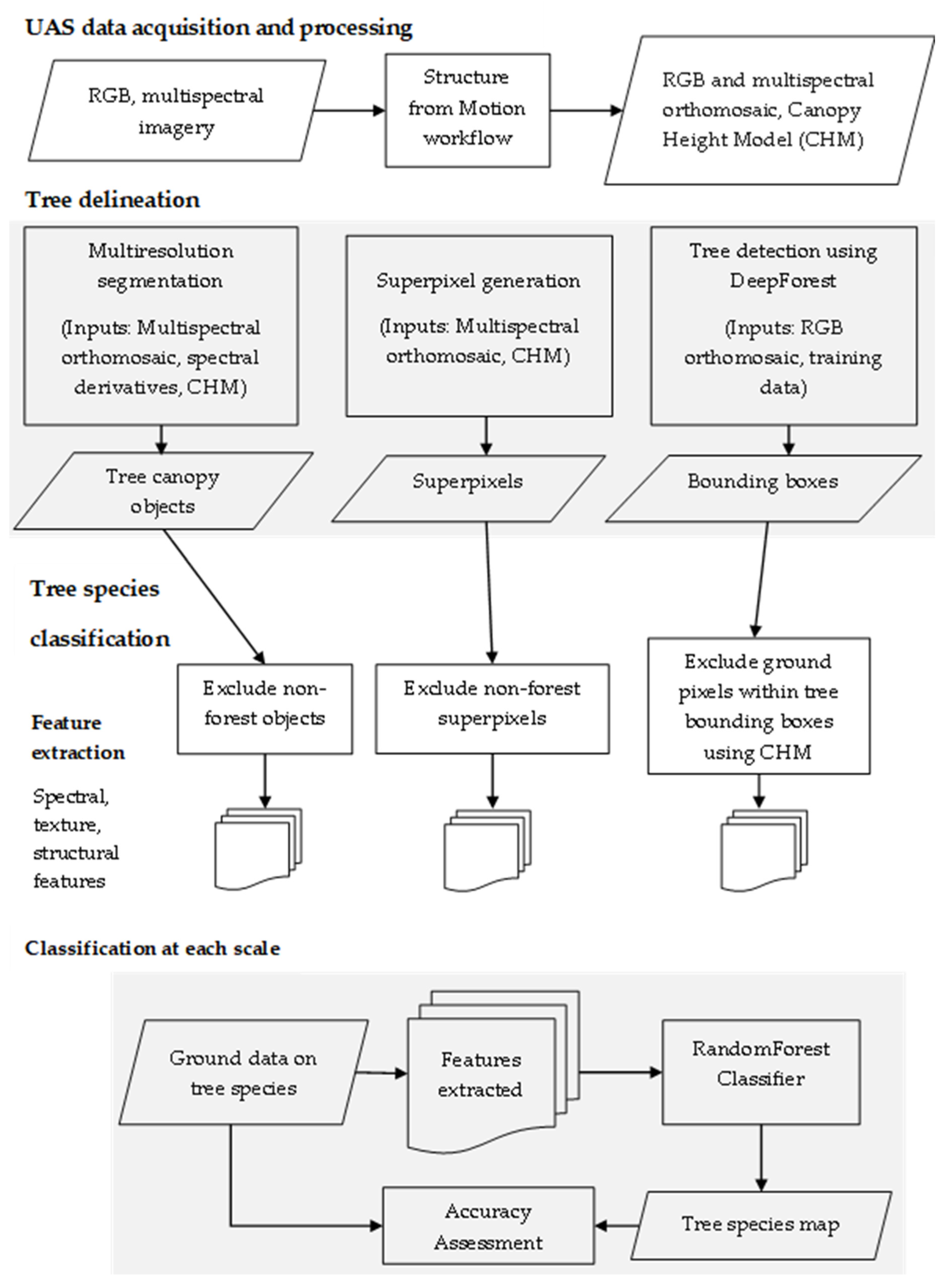
An overview of the methods used in this study is shown in Figure 1. UAS RGB and multispectral imagery were processed in a Structure from Motion workflow to generate RGB and multispectral orthomosaic and a Canopy Height Model (CHM). Tree canopies were extracted at three scales using: (i) multiresolution segmentation (MRS), (ii) superpixels, and (iii) individual tree bounding boxes using DeepForest. At each of these scales, features were extracted for the forested areas. Ground data on tree species and the extracted features were used in a RandomForest classification workflow to generate tree species maps and to validate the classification results.

2.1. Study Site

The study area is a dry sclerophyll forest located near Swansea in the East Coast region of Tasmania, Australia. The site was selected as it has been used for long-term ecological monitoring by plant physiologists to study drought tolerance and the post-drought recovery process at the plant level [42]. Terrain elevations range from 105 to 171 m above mean sea level. Vegetation communities in the study area include the open, dry Eucalyptus pulchella-dominated forest, dense Callitris rhomboidea forest, and tall, dense shrub dominated by Melaleuca pustulata. The dominant overstory tree species are Eucalyptus pulchella, Eucalyptus viminalis, Callitris rhomboidea, Acacia mearnsii, and Allocasuarina verticillata. Other overstory species include Exocarpos cupressiformis, Eucalyptus globulus, and Allocasuarina littoralis.
Figure 1. Flowchart of the workflow used for tree canopy delineation and tree species classification at the object, superpixel, and individual tree bounding box scales.
Remotesensing 14 04963 g001

2.2. Data Acquisition and Processing

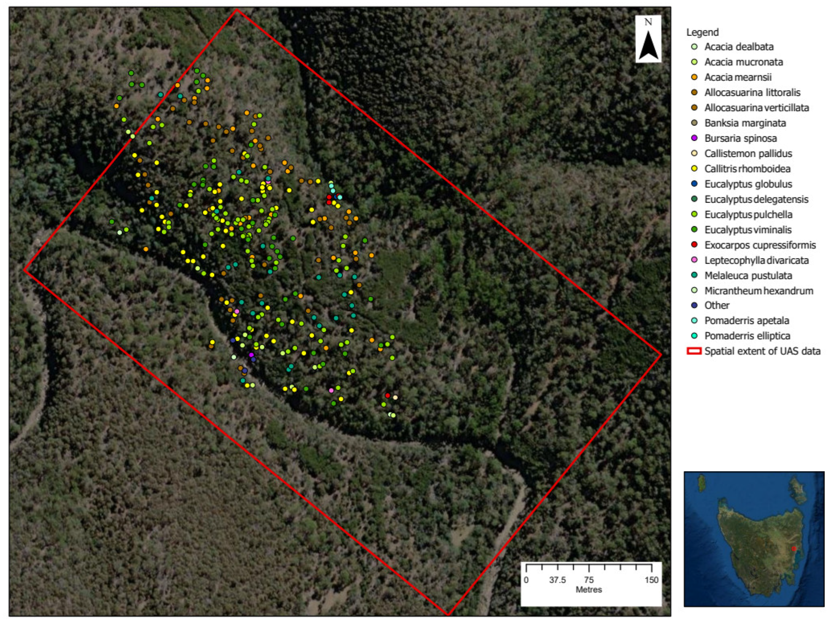
The datasets used in this study included multispectral images from the MicaSense RedEdge-MX sensor that were captured by flying a DJI Phantom 4 Pro at a height of 110 m with 90% forward and 80% side overlap in 5 flights. The RedEdge-MX sensor captures 5 bands: Blue, Green, Red, Red Edge, and NIR. The sensor has a focal length of 5.5 mm, the horizontal field of view is 47.2°, and vertical field of view is 35.4°. The MicaSense calibrated reflectance panel (CRP) was used to convert raw pixel values to reflectance using CRP images captured before and after the flight. RGB images were also acquired using the DJI Phantom 4 Pro. Ground Control Points (GCPs) were placed in relatively open areas across the site and located using a survey-grade Real-Time Kinematic (RTK) Global Navigation Satellite System (GNSS) and were used to georeference the imagery. A total of 314 tree species records (Figure 2) were collected on the ground for the training and validation of species classification.
Agisoft Metashape Professional (v 1.6.4) software was used to generate RGB and multispectral orthomosaic (resolution 5 cm). A CHM was generated at 5 cm resolution using the high-resolution surface model from RGB dense point cloud and digital elevation model (DEM) from lidar data. The CHM was generated from SfM RGB imagery so that the height model perfectly matched the orthomosaic. The ground points from an independently collected UAS lidar point cloud were used as the bare ground height was better captured in the lidar data compared to the SfM point cloud.
Figure 2. Inset map shows location of study site in the East Coast region of Tasmania. Map shows spatial extent of UAS data and ground data points on tree species.
Remotesensing 14 04963 g002

2.3. Tree Segmentation

2.3.1. Multiresolution Segmentation

MRS was used for detection of individual tree objects. MRS is a region-growing algorithm where adjoining pixels are grouped based on similarities in image characteristics (e.g., reflectance and height). Homogeneity criteria were defined using several parameters: scale, shape/color, compactness/smoothness, input layers, and weights. The following input layers were used: five spectral bands (R, G, B, NIR, and Red Edge), normalized ratios of scaled RE, NIR and B [4], and Red Blue NDVI ((NIR − (R-B))/(NIR + (R-B)) [43] and CHM. A range of values were tested using subsets of the study area, and the results were visually inspected to tune the parameters. Based on this visual inspection, a weight of 5 was set to the CHM to avoid mixing between ground and canopy in the resulting objects. The scale defines the maximum allowed heterogeneity for the resulting canopy segments. A scale of 30 was found to be appropriate as it did not result in mixed segments. Default values were used for Shape (0.1) and Compactness (0.5). Shape defines the relative weight of shape compared to the input layer values. Compactness defines the relative weight of compactness compared to smoothness of the image objects.

2.3.2. Superpixels

Superpixel segmentation creates objects that are regular in size throughout the image and efficiently groups pixels into perceptually meaningful regions [44]. Superpixels carry more information than a pixel and represent a scale between individual pixels and tree canopy image objects. Achanta et al. [25] proposed a new gradient-ascent-based method, Simple Linear Iterative Clustering (SLIC), an adaptation of k-means clustering for superpixel generation. The algorithm uses a single parameter, k, the number of equally sized superpixels to be created and an optional compactness parameter. k initial cluster centers are generated on a regular grid spaced S pixels apart (dimension of the superpixel). Unlike k-means clustering where distances are calculated to every pixel in the image, the search space was limited to a 2S × 2S region around the center. In an iterative procedure, every pixel was assigned to the nearest cluster. Compared to five other superpixel methods, SLIC was found to perform the best with respect to boundary adherence, speed, and undersegmentation error. While SLIC is sensitive to texture and generates smooth regular-sized objects in non-textured regions and irregular objects in textured regions, the parameter-free version SLICO generates regular-sized superpixels across the image [25].
In this study, we used the SLICO the zero-parameter version in eCognition to generate superpixels. The following Input Layers were used: five multispectral bands—R, G, B, NIR, and Red Edge—and the CHM. The CHM was scaled between 0 and 1, to match the spectral band range. The average size of the superpixel objects was tuned in increments of 5 pixels (Region Size ranging from 10 to 65) to identify an optimal segment size while ensuring there was no undersegmentation. Default values were used for Iterations, Enforce Label connectivity and Minimum Element Size.

2.4. Tree detection Using DeepForest

Studying DL models to detect trees across different sites, Weinstein et al. [45] found that models performed better when trained with data from other sites and combined with a relatively small dataset from the study site. The DeepForest package supports the transfer learning strategy where the entire model is re-trained with additional data. The strategy of freezing the initial layers and fine-tuning of only the last layers using site-specific imagery was not supported in the DeepForest model used in this study. The usefulness of transfer learning methods depends on the task. Exhaustive training using site-specific data might result in higher accuracy than using generic datasets to train the model [32]. However, as training data specific to Eucalyptus forests was scarce and considering the scope of this study, we tested the following two approaches for individual tree detection using DeepForest. First, the pre-built DeepForest model was used with default settings. The second approach was to train the pre-built model with bounding box annotations from the study area to match the UAS data resolution. DeepForest open-source Python package (v0.3.7) [41] was installed in a dedicated environment in Anaconda [46]; Jupyter notebook was used to code and visualize the results.
The pre-built model in DeepForest was trained using airborne lidar and RGB data [41]. This model was used to detect (with predict_tile) tree crowns in a test subset in the study area.
The pre-built model can be trained with data from the study area. A training subset was defined to include different types of canopies in the study site, and bounding boxes were defined using ArcGIS Pro (v 2.7.1) for all trees and large shrubs. The training subset raster was trimmed to only include the extent of the annotated bounding boxes (Figure 3) and was exported as a TIF file. The bounding box feature class containing 143 records was exported to the format required by DeepForest. The training raster was split into smaller windows. Patch_size and patch_overlap determine the size and overlap between the windows. Weinstein et al., authors of the DeepForest package, [41] used 400 pixel image patches on 10 cm resolution airborne data to train the pre-built model, but with finer resolution data, larger patches are required to capture trees. Patch_size values of 600, 800, 1000 pixels were tested to train and predict the test data. In the DeepForest model used in this study, no observable impact on accuracy was found and 1000 pixels was chosen. Weinstein et al. [41] stated that the patch_size parameter is less likely to have an impact when the model is re-trained on data from the site than when used with the pre-built model to predict trees captured at resolutions different to what the model was trained on (10 cm/pixel). Patch_overlap was set as a percent overlap and the default value 0.05 was used. The epochs parameter was updated to 10 (from the default value of 1) to increase the number of iterations of training. Epoch values from 5 to 10 were found to be sufficient for small training datasets [41]. The default settings were used for other model parameters in the DeepForest configuration file used to train and validate the model.

Validation

Validation was essential to test the accuracy of the pre-built model and to assess improvements with training using data from the site. Evaluation functions in DeepForest calculate mAP, which combines precision and recall in a single metric measuring the area under the precision–recall curve resulting in a score from 0 to 1. The Intersection over Union (IoU) threshold (the area of overlap by the area of union between the predicted and the hand-annotated bounding box) was used to identify if a prediction is a true positive. The default threshold was used, so predictions were considered true positives if the IoU was at least 0.5. Evaluate_generator was used to calculate the training accuracy (mAP) to identify how well the model predicted the training data. Training for additional epochs is suggested [41] when the mAP is less than 0.5. So, the training accuracy and visual assessment of the prediction results were used to identify whether more training was necessary.
Three test subsets were identified separate to the training data (Figure 3). As with the training data, 151 trees in the three subsets (overlapping canopies: 77; dense closed canopies: 38; and canopies distinct from background: 36) were annotated using ArcGIS Pro and converted to the required csv format in Python. The testing tiles were split into overlapping windows of size 1000 pixels. These annotations were passed to the DeepForest model during training (validation_annotations) to visualize the change in accuracy at the end of each epoch, and to tune the number of epochs. As with the training accuracy, evaluate_generator was used to calculate mAP test accuracy and predict_tile was used to generate bounding box predictions across the site. The predicted individual tree bounding boxes were georeferenced and converted to Shapefile format using geopandas for subsequent analysis.

2.5. Tree Species Classification

2.5.1. Spectral Features

The mean and standard deviation of spectral bands and vegetation indices (VIs) (Table 1) were calculated at each scale of analysis. Previous studies compared the use of spectra from all pixels in a canopy with spectra using brighter pixels only [7,8,18]. In this paper, the following approaches were tested to assess the impact on classification accuracy:
4.
Spectra extracted from all pixels within the canopy.
5.
Spectra extracted only from pixels with SR (which is NIR/R) above the mean value in the tree canopy. This was performed to address the mixing of bare ground and canopy gaps at all scales of analysis.
At the individual tree bounding box scale, all features used in the classification workflow were extracted only for the canopy pixels. The CHM was used to exclude ground pixels in the bounding boxes.

2.5.2. Texture Features

Texture measures can provide valuable information on spatial patterns and assist in the classification of tree species [24,29]. The window size used to calculate texture measures has an impact on the usefulness of the features in classification: small windows may amplify differences while larger windows smooth the variation and cannot effectively extract texture information. Eight texture measures based on the grey level co-occurrence matrix (GLCM) [47] were calculated at (i) the pixel-level for use with the DeepForest bounding boxes and (ii) at the object-level for MRS objects and superpixels (Table 1). The NIR band (scaled to 8 bit) was used for the GLCM calculations as it is most sensitive to variations in vegetation. Pixel-level measurements were generated in ENVI with a window size of 5 × 5 pixels (default shift of 1 pixel in X, Y) based on visual inspection using a test mosaic of the dominant classes. Object-level measurements were calculated using the performance-optimized version of Texture after Haralick in eCognition (‘quick 8/11’) [48].

2.5.3. Structural Features

In addition to spectral and texture features, structural features might assist with species classification. Two sets of structural features were calculated from the photogrammetric point cloud: CHM statistics (mean and standard deviation of normalized height values) and structural metrics derived from the point cloud. For the latter, lascanopy from LAStools [49] was used with DeepForest tree bounding boxes and MRS objects to generate structural metrics (Table 1). As superpixels captured smaller elements of the tree canopy, point cloud metrics were not applicable at this scale.
Table 1. List of features used in Random Forest classification for the three scales of analysis. Features were calculated at all scales of analysis unless indicated otherwise.
ClassFeatureFormulaStudy
Spectral
(Mean and Standard
Deviation)
All multispectral bands: B, G, R, RE, and NIR
Normalized ratios of scaled B, RE, and NIRcx/(cNIR + cRE + cB)
where cx is one of cNIR, cRE, cB relative reflectance stretched to RGB colour space (0–255)
[4]
NDVI(NIR − R)/(NIR + R)
Red Blue NDVI (RBNDVI)(NIR − (R − B))/(NIR + (R − B))[43]
Normalized Difference RedEdge Index (NDRE)(NIR − RE)/(NIR + RE)[29]
Modified Canopy Chlorophyll Content Index (M3CI)(NIR + R − RE)/
(NIR − R + RE)
Plant Senescence Reflectance Index (PSRI)(R − G)/RE
Chlorophyll Index RedEdge (CIRE)(NIR/RE) − 1
Green NDVI(G − NIR)/(G + NIR)[20]
Normalized Green Red Vegetation Index (NGRVI)(G − R)/(G + R)
Normalized Green Blue Index (NGBI)(G − B)/(G + B)
Normalized Red Blue Index (NRBI)(R − B)/(R + B)
Simple RatioNIR/R
Green Vegetation IndexNIR/G
Object-level texture
(Scales: superpixel, object)
GLCM co-occurrence measures on NIR band:
mean, standard deviation, contrast, dissimilarity, homogeneity, angular second moment, entropy, and correlation.
Direction 135° to match the pixel-level texture calculated with direction shift X, Y: 1, 1. In the eCognition implementation of Haralick texture, 0° represents the vertical direction and 90° represents the horizontal direction.[47,48]
Pixel-level
texture
(Scale:
bounding box)
As above. ‘Mean’ of each measure extracted from bounding box. Window size 5 pixels, direction shift: X,Y: 1,1.[47]
CHMMean and standard deviation CHM
Structural
metrics
(Scales: object, bounding box)
Metrics derived from the photogrammetric point cloud: canopy cover, skewness, minimum, square of average height, average, maximum, standard deviation, kurtosis, and vertical complexity.Default height cut-off of 1.3 m
Shape
(Scale: object)
Border index, roundness, compactness, shape index, rectangular fit, and asymmetryObject-level features

2.5.4. RandomForest Classification

Eucalyptus viminalis and Eucalyptus pulchella form mixed stands in the study site. There is diversity in growth stages in both species, and structural variability in E viminalis (healthy canopies as well as crowns with foliage loss). E viminalis is vulnerable to water stress and shows substantial foliage loss and crown death when stressed, whereas E pulchella is relatively unaffected [50]. Hence, there is value in being able to distinguish between the two Eucalyptus species with respect to monitoring changes due to water stress. Previous studies classified individual Eucalyptus species and a combined Eucalyptus class with mixed results, depending on the variability of the species on the site [7,8]. In this study, the individual Eucalyptus species were classified separately (Table 2). In addition, the two Eucalyptus species were grouped in a class, and classification performed using the best set of input features identified at each scale.
Classification was performed only in forested areas using a mask to exclude other areas. Non-forest areas were excluded using thresholds on CHM and Forest Discrimination Index (FDI = NIR − (RE + B)), which is zero or negative for non-forest and dry vegetation. The RandomForestClassifier in Python-based sklearn (0.23.2) [51] was used for classification. The main parameters in this classifier are num_estimators (number of trees) and max_features. Num_estimators was set to 500 and the default value (square root of total number of input features) was used for max_features. RandomForestClassifier has Bootstrap enabled by default and each new tree was fitted using a bootstrap sample of the training set. Oob_score was set to True to use out-of-bag samples to estimate a generalisation score. Ground data were split into training (80%) and test (20%) sets (train_test_split with the same random_state value for consistency) to fit the model. The feature combinations shown in Table 2 were tested to assess the impact on accuracy.
Table 2. Feature combinations used at the three scales of analysis.
Scale of AnalysisFeature CombinationClasses
SuperpixelsSpectral, CHM Acacia mearnsii,
Allocasuarina spp.,
Callitris rhomboidea, Eucalyptus pulchella, Eucalyptus viminalis, Melaleuca pustulata,
‘Other Vegetation’
Spectral, CHM, object-level Texture
MRSSpectral, CHM metrics
Spectral, CHM, object-level Texture
Spectral, CHM, shape
Spectral, CHM, PPC metrics
Spectral, CHM, object-level Texture, shape, PPC metrics
DeepForestSpectral, CHM metrics
Spectral, CHM, pixel-level Texture
Spectral, CHM, PPC metrics
Spectral, CHM, pixel-level Texture, PPC metrics

2.5.5. Feature Importance

The most important features to explain the model outcome can be calculated using two approaches in RandomForestClassifier: feature importance and permutation-based feature importance. The default fitted attribute feature_importances_ is calculated based on the contribution of each feature to the mean decrease in impurity. Permutation-based feature importance is the mean decrease in model accuracy when a feature value is randomly shuffled. The most important features to make predictions were identified using both feature_importances_ and permutation-based importance. Permutation_importance was used with the fitted model and training dataset to permutate features 10 times (n_repeats). Although the test set could be used for permutation-based importance, the training set was used in this paper due to the larger number of samples. This approach also enabled comparing the two importance measures.
Feature importance measures indicate which features are most relevant for a particular model, and do not imply that these features are better predictors of the outcome over other correlated ones. When features are correlated, although any of them can be among the more important variables when one of the features is used, the importance of others will be reduced. For example, when one of the correlated features is randomly permutated, the model can obtain the same information from related features, and hence not have an impact on the accuracy. Several of the features discussed in the previous section are correlated (e.g., texture measures and VIs). Prior to fitting the RandomForest model, hierarchical clustering using Spearman’s rank correlation was used to visualize the correlated features, and a single feature from each cluster was selected (based on a distance of 1). The model was fitted using this subset of features.

2.5.6. Classification Accuracy Assessment

Overall class-specific metrics were calculated using classification_report and confusion_matrix (sklearn metrics). Precision (producer accuracy) is the proportion of trees that belong to a class among all those that were classified as that class.
precision = tp/(tp + fp)
where tp is the number of true positives and fp the number of false positives.
Recall (user accuracy) is the proportion of trees that were classified as a class among all trees that truly belong to that class.
recall = tp/(tp + fn)
where tp is the number of true positives and fn the number of false negatives.
F-score is the harmonic mean of Recall and Precision.
F-score = 2 × (precision × recall)/(precision + recall)
In addition, on the model with highest overall classification accuracy, spatial variability and classification uncertainty were visualized using Confusion Index and species probability layers. The Confusion index in ratio form [52] was calculated to identify areas where classification was least certain:
Confusion Index = MaxProb2/MaxProb
where MaxProb and MaxProb2 are the maximum and second highest probability values at each location.

3. Results

3.1. Multiresolution Segmentation

Tree canopy objects generated with MRS are shown in Figure 4. Input layers and segmentation parameters with the highest segmentation accuracies across the three canopy subsets were used. Tree canopies in open areas where there was a distinct difference between background and crown were delineated better with segments resembling visually interpreted tree crowns (Figure 4A). On the other hand, branching Eucalyptus spp. canopies were oversegmented (Figure 4B); dense, overlapping canopies of different species were combined in a single segment (Figure 4B). However, the results were mixed across the site. Visibly distinct trees and with a well-defined canopy structure were nevertheless undersegmented, for example, mixing of Callitris rhomboidea crown and neighbouring Eucalyptus pulchella branches (Figure 4C).

3.2. Superpixel Generation

Superpixels were generated using SLICO with the five spectral bands and CHM. Region size values from 10 (default) to 65 were tested in increments of five. Sizes 10, 35, and 55 are shown in Figure 5. The default value of 10 oversegmented the image; with size 35, the boundaries between classes were retained and oversegmentation was reduced. With sizes larger than 35, while oversegmentation was further reduced in tree canopies that were distinct from the background (i in Figure 5C), most areas were undersegmented. Mixing occurred between ground and canopy edges (ii in Figure 5C), and between overlapping canopies of different species, for example, Eucalyptus spp. and Acacia mearnsii canopies (iii in Figure 5C). Superpixels generated with region size 35 were used in the subsequent analysis.

3.3. DeepForest

3.3.1. Pre-Built Model

Predictions using the pre-built model and default settings are shown in Figure 6A. Parts of tree canopies and ground were predicted to be trees. This is likely due to two main reasons. The pre-built model was trained on coarser resolution data (10 cm/pixel) [41] compared to the UAS imagery used in this paper (5 cm/pixel). In addition, the default patch_size used to split the tile was 400 pixels, which might explain the smaller tree bounding boxes. The test accuracies are listed in Table 3.

3.3.2. Trained Model

Training using the RGB orthomosaic of the site improved model performance considerably (Table 3). Training and test accuracies (mAP) were over 0.8 with both datasets. Test accuracies ranged from 0.65 in well-spaced trees distinct between background to ~0.5 in more complex open Pulchella forest, and closed canopy Callitris forest.

3.3.3. Tree Detection in Mixed and Closed Canopies
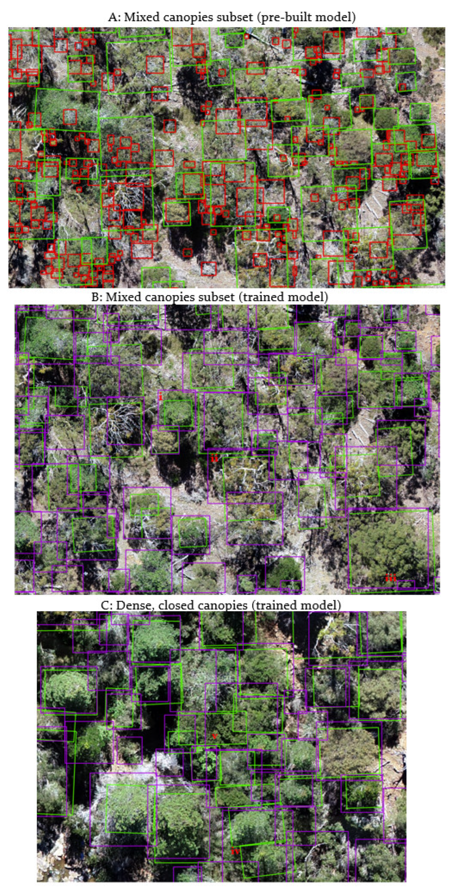
Predictions and test boxes for mixed canopies and dense, closed canopy subsets are shown in Figure 6. mAP combines the Recall and Precision metrics and is indicative of overall performance. Test accuracies in these canopies was around 0.5 and higher (0.65) in canopies where trees were distinct from background. The results were visually inspected to identify areas where trees were undetected and those where the spatial extent of the detected trees was poor. In dense, overlapping canopies, digitizing the test data was challenging, and in most cases, the predicted spatial extent was larger than the test extent ((i) in Figure 6B). Parts of branching Eucalyptus canopies were detected multiple times (oversegmented) ((ii) in Figure 6B). The edges of canopies and understory were detected separately ((iii) in Figure 6B). In closed, dense canopies, tree crowns close together were missed ((iv) in Figure 6C). Trees in the middle of dense scrub in this subset were detected ((v) in Figure 6C); however, across the site, the difficulty in digitizing dense scrub extent using bounding boxes resulted in individual trees in dense scrub being undetected.
Figure 6. Predictions from DeepForest overlaid with manually delineated test data (in green). (A) Bounding box predictions (in red) using the DeepForest pre-built model overlaid with the manually delineated test data. (B) Predictions from DeepForest model trained with data from the site. Digitizing tree extent was challenging in overlapping canopies. Additionally, in several instances, (i) the predicted extents were larger than the digitized test box. Branching canopies were split into multiple boxes (ii). The edges of canopies were detected in several, small spurious polygons (iii). (C) In the closed canopy Callitris forest, crowns close together were grouped within a box (iv). Digitizing dense Melaleuca pustulata scrub extent in bounding box format was also challenging and caused mismatches in the predicted results (v). However, all tree crowns around this low-lying scrub were detected in this instance.
Remotesensing 14 04963 g006

3.4. RandomForest Classification

3.4.1. Classification Accuracy

Classification using RandomForest was performed with various feature combinations. Firstly, to address the mixing of ground and canopy gaps with tree canopy elements, two methods were tested. Classification using spectra extracted from all pixels within the canopy was compared with results from using spectra only from pixels with SR greater than the average within the canopy (Table 4). Results from spectra filtered using average SR are reported for the rest of the analysis. Results with additional feature combinations are summarized in Table 5. The highest classification accuracy was achieved at the superpixel scale (0.84), followed by the object scale (0.77) and bounding box (0.69). Input features with the highest classification accuracy were used to calculate classification accuracy with the two Eucalyptus spp. grouped. With Eucalyptus aggregated, accuracy at the superpixel scale improved (0.93). At the bounding box scale, classification accuracy with grouped Eucalyptus improved and was comparable to that achieved at the object scale (0.77). There was no improvement in overall accuracy at the object scale.

3.4.2. Class-Specific Accuracies

Class-specific metrics on the best performing model at each scale are shown in Table 6 (Melaleuca pustulata shrub and ‘Other’ classes not displayed here). Acacia mearnsii, Allocasuarina spp., and Callitris rhomboidea were best classified at the superpixel scale (F-Score over 0.9). Both the Eucalyptus species had the highest F-scores at the object level (E pulchella: 0.85, E viminalis: 0.79). Callitris rhomboidea was classified with similar accuracy for the objects and bounding boxes (~0.82).
Combining the Eucalyptus spp. in a class (Table 7) improved Eucalyptus spp. accuracies and hence overall accuracies with superpixels (0.92) and bounding boxes (0.89). At the object scale (0.77), there was no improvement where Eucalyptus spp. Precision (0.73) was negatively impacted due to the misclassification of species (Acacia mearnsii and Allocasuarina spp.) as Eucalyptus.

3.4.3. Important Features

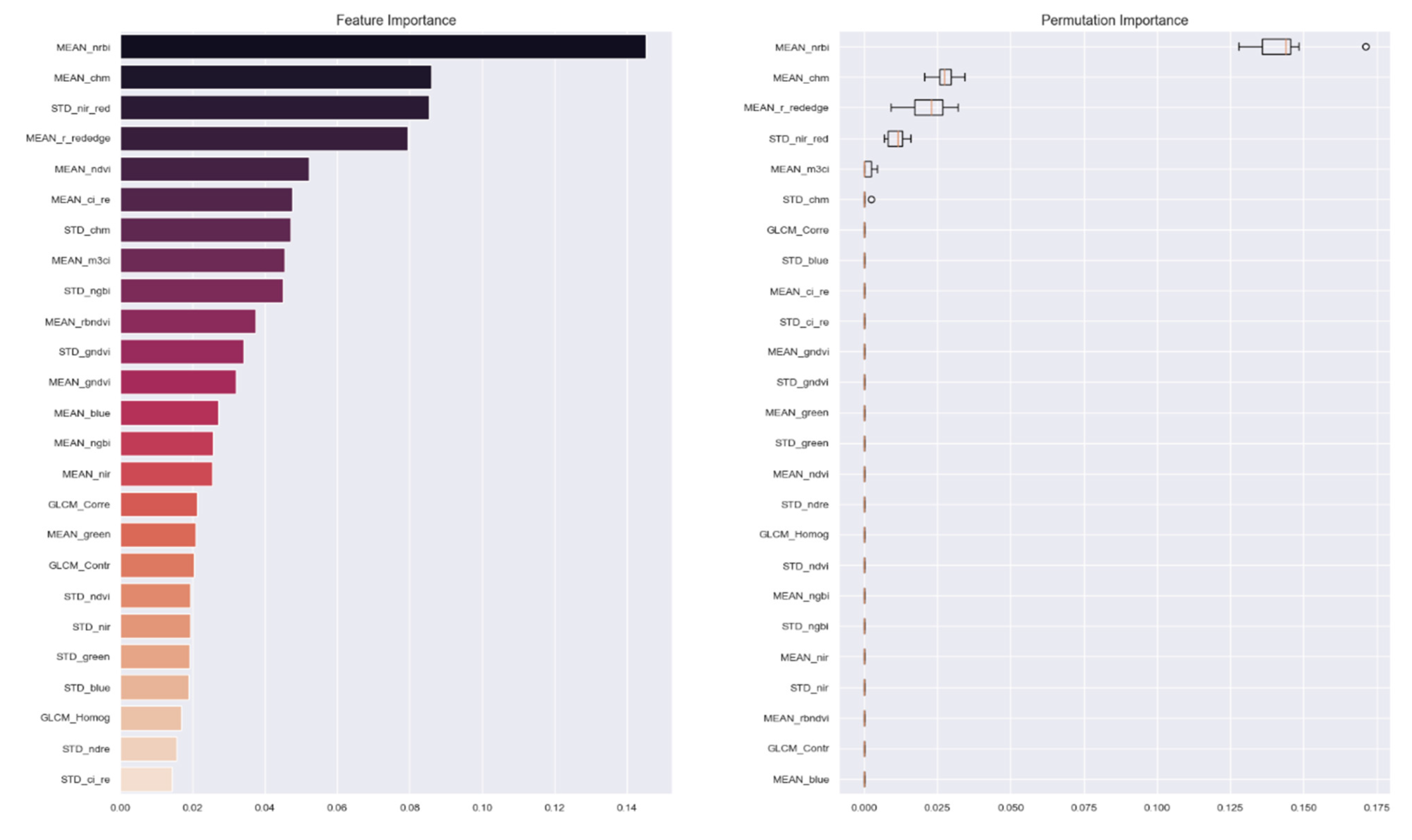
Prior to fitting models, some of the correlated features were removed using Spearman’s rank correlation and a threshold of cluster distance using hierarchical clustering. Feature and permutation importance for the model with the highest classification accuracy (superpixel scale with the Eucalyptus classes aggregated) are shown in Figure 7. Using either measure, spectral indices and the CHM were the most relevant features for this model. Mean NRBI and CHM were the most relevant by either importance measure. The mean of the normalized RE ratio (MEAN_r_rededge) and standard deviation in SR (STD_nir_red) were in the top five important features by either importance measure but were ranked differently. Permutating MEAN_m3ci was found to have a marginal impact on accuracy, whereas feature importance scores indicated more features to be relevant and, based on permutation only, five features had an impact on accuracy. Features were permutated 10 times and the mean decrease in accuracy was calculated on the training dataset. The boxes in the permutation importance plot indicate the interquartile range of the mean decrease in accuracy from the RandomForest repeats. The orange line in the boxplot (Figure 7) indicates the median decrease in accuracy (any outliers are shown as dots).
Permutating NRBI (mean) dropped the accuracy by nearly 0.15, and permutating CHM (mean) and normalized RE ratio (MEAN_r_rededge) reduced the accuracy by around 0.025 (Figure 7). Permutating SR and M3CI features had a marginal impact on the accuracy.
In the best performing models at each scale, the most relevant features were similar using both the feature and permutation importance; fewer features had non-zero permutation importance (Figure 7). Permutation-based importance can be calculated on a held-out test dataset (not performed here due to fewer samples in the test set), can be used to measure decrease in accuracy metrics other than the default mean accuracy, and is robust against high cardinality unlike impurity-based importance. Hence, the most relevant features based on permutation-based importance are shown in Table 8. Spectral derivatives and CHM were the most important features. NRBI, r_rededge (normalised ratio of scaled RE) and CHM were relevant at all scales. At the object and bounding box scales, derivatives based on the RE band were also important (CIRE, M3CI, and PSRI).

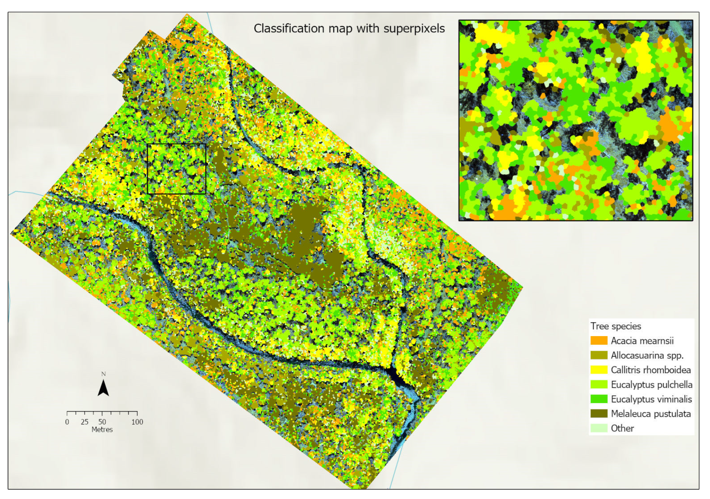
3.4.4. Classification Maps

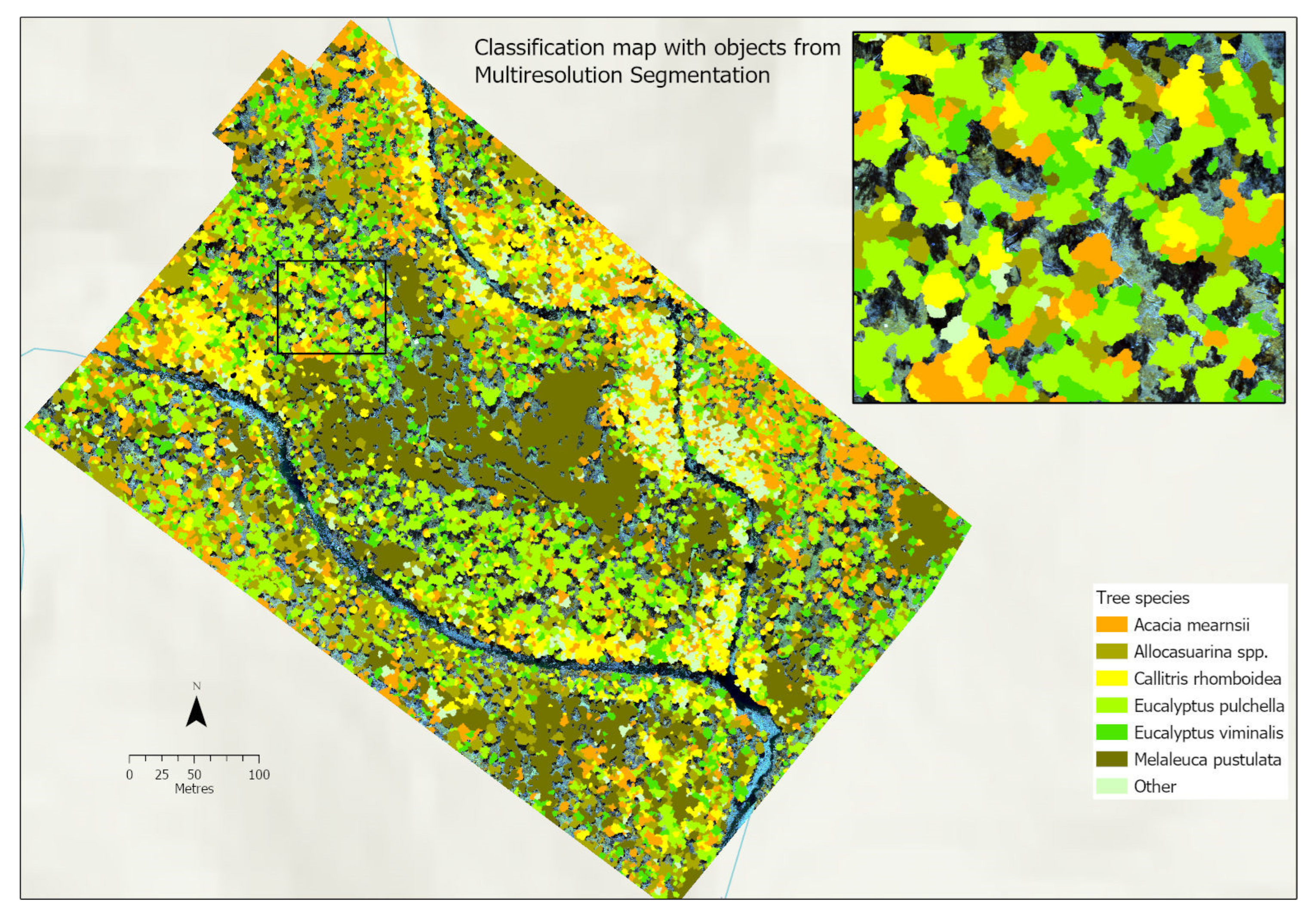
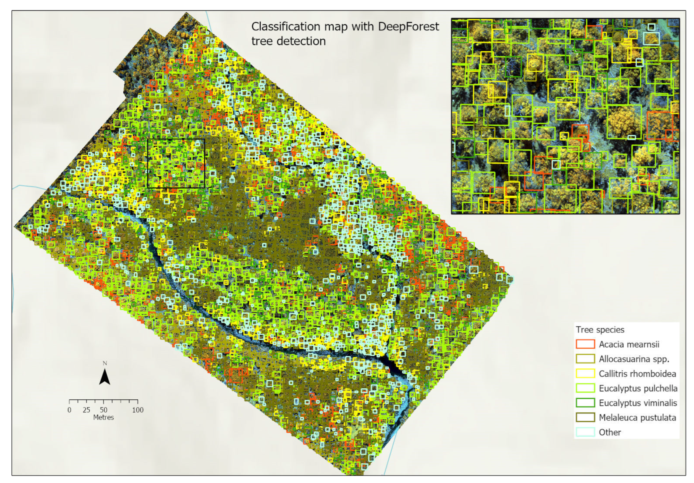
Tree species classification maps generated at the three scales are shown in Figure 8, Figure 9 and Figure 10. A subset of the study area Pulchella dominated forest is shown in the inset. From the results at the superpixel scale (Figure 8), it is evident that oversegmentation led to ‘speckles’ across the site (similar to that observed in pixel-based classification of high-resolution imagery). Differences in illumination, gaps, or shadows in the canopies resulted in the misclassification of canopy edges, and these can be observed as speckles. This effect is present, although less prevalent, using objects generated from MRS (Figure 9), where the scale of analysis is coarser and corresponds to larger parts of tree canopies. The classification map generated at the individual tree scale is shown in Figure 10. Trees distinct from the background were detected better than those in dense canopies, and this is evident from the results across the site (for example, in the inset, trees with distinct gaps around the crowns were classified correctly). The erroneous detections of canopy edges led to the misclassifications of these spurious detections as ‘Other’.
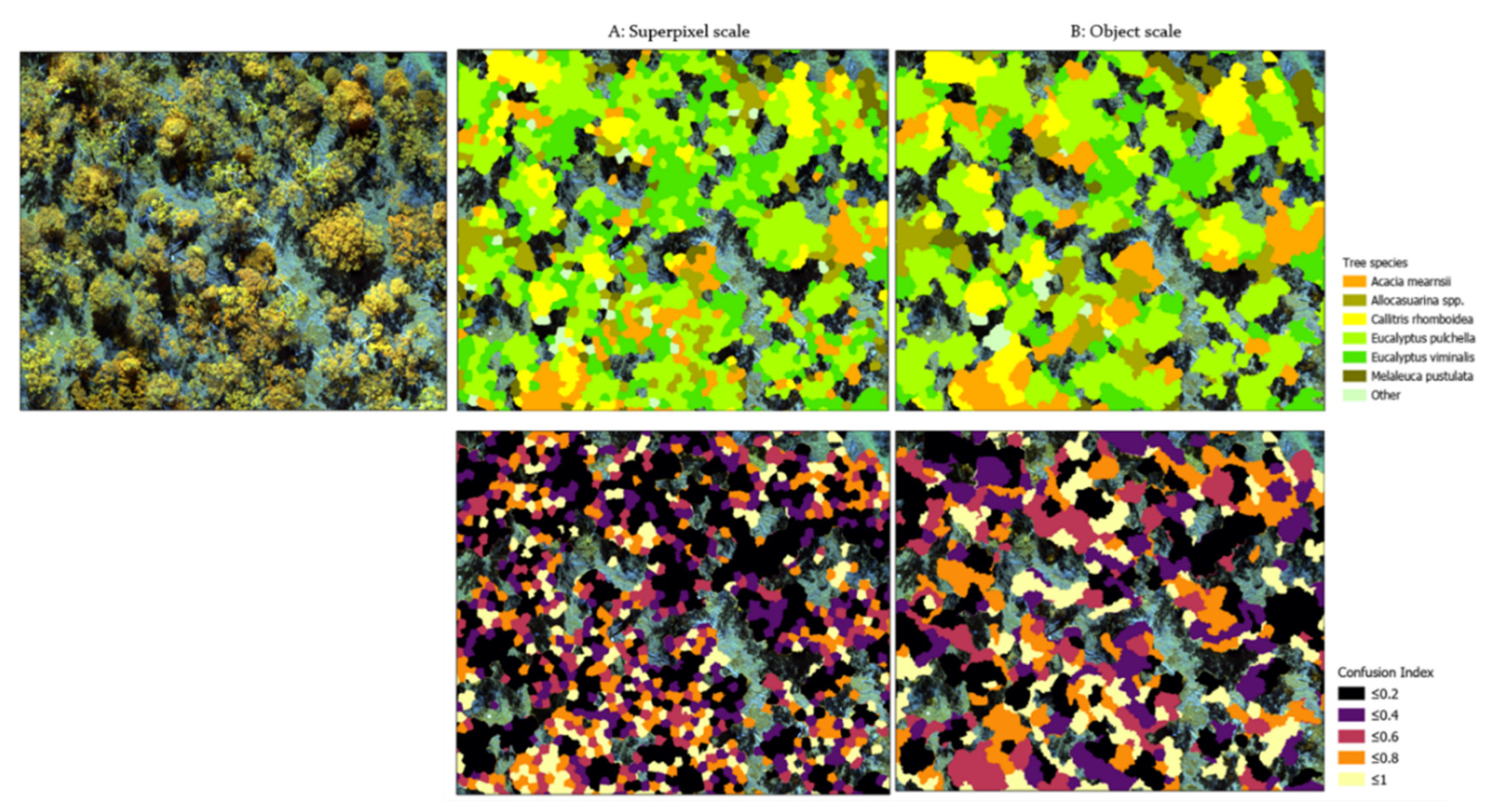
Probability maps were generated using the predicted class probabilities from models with the highest classification accuracies. Areas indicating high probability of a species could be used to direct data collection efforts. In addition, the Confusion Index was used to visualize the spatial variation in classification uncertainty (Figure 11). This value (ratio of maximum and second highest probability values) can be interpreted as the confidence in the prediction. Values closer to 1 indicate similar probabilities in the top two classes and hence low confidence in the prediction, whereas values closer to zero indicate the top class had a higher probability than the second highest, and hence less confusion between classes. Predictions from the model and the Confusion Index are shown at the superpixel and object scales (Figure 11). No class-specific relation is evident by visually comparing the predicted class and associated Confusion Index. These maps show that, although the model accuracies were high, confidence in the predicted classes was not. For example, at the superpixel model with the highest accuracy, 67% of superpixels had a Confusion Index over 0.3. This is indicative of the spectral similarity between the tree species in this forest, and perhaps highlights the need for additional training data, or input features to improve confidence in the classification.

4. Discussion

4.1. Tree Detection with DeepForest

In this study, a workflow was implemented to use the DeepForest package with high resolution UAS RGB imagery. Training the pre-built model with a small dataset from the site considerably improved the results. A training accuracy of 0.82 was achieved, while test accuracies were 0.65 in the closed canopies subset and 0.5 in the dense and overlapping canopies subsets. A mAP score above 0.5 has been suggested as usable for scientific applications [41]. The trained model was validated using mAP, which combines Recall and Precision. mAP was found to be the lowest in overlapping Eucalyptus canopies and the highest in open areas where trees were distinct from background. Trees were undetected (multiple trees detected in a single bounding box) in dense, overlapping canopies. Some of these errors were likely due to the branching structure, but this was also observed with tree crowns with a distinct treetop structure, e.g., in the Callitris forest (Figure 6C). These errors were likely due to limitations in training data as well as the use of only RGB for tree detection. Digitizing tree extent using bounding boxes was challenging especially for branching forms without a well-defined treetop center, such as Acacia mearnsii, and for dense scrub. This is likely to have impacted model predictions. Detecting and delineating trees in multi-layered, overlapping canopies requires the ability to discriminate between tree species (e.g., spectral differences, crown architecture, and canopy density). Model performance could be improved with (i) additional training cycles, (ii) increasing training data specific to problem areas, and (iii) using data augmentation (rotation and brightness transformation), but will involve additional processing time. The pre-built DeepForest model was trained using NEON, a database of field sites across the USA. Similarly, a database of Australian native tree species might assist in transfer learning techniques and improve tree detection in these forests.
While only the mAP metric available through DeepForest package was used to validate results here, Weinstein et al. [45] calculated Precision and Recall and identified areas where tree detections were missed and where the spatial extent was poorly delineated. It was found that additional training data improved the predictions of tree crown boundaries but not tree detections. Tree detection accuracy was the highest when models trained with data from various sites were re-trained with a small dataset from the local site (cross-site learning) [45].
DeepForest offers a transferable and generalized solution to individual tree detection and can be used to establish a baseline map to study overall change with time. However, improvements to the model as discussed above might be necessary to better delineate trees for applications where individual tree detection is required to link remotely sensed data to ground data, for example, to study genetic differences in species [53], or to monitor individual tree health [43].

4.2. Scale of Analysis and Classification Accuracy

The scale of analysis for tree species classification can vary from tree canopy pixel, or pixels grouped to a tree canopy object to individual tree crowns. In this study, three scales of tree canopies were generated for classification: superpixels, objects, and bounding boxes. It must be noted that, while comparing classification accuracies between these scales, the number of training/validation samples used at each scale was different as: (i) there was mixing of canopies at bounding box and object scales, and hence not all trees in the reference dataset were used at these scales; and (ii) with superpixels, field samples that were collected at the tree level were manually copied to cover the canopy to generate adequate training data at this scale.
The highest overall accuracies were achieved with superpixels (84% with seven classes and 93% with six classes of Eucalyptus species aggregated). Oversegmentation reduced the mixing of species within the canopy and improved classification. One of the objectives of this study was to identify whether oversegmentation through superpixels can be used to discriminate species with similar levels of accuracy as conventional image segmentation, such as MRS. Oversegmentation can be advantageous when the clumps are separable; however, when species are more separable at a coarser scale, as was likely the case with the two Eucalyptus species in the site, a small scale can negatively impact classification. With grouped Eucalyptus, the F-score improved considerably (0.92 compared to 0.66). It must be noted that, unlike bounding box and object scales, training and validation samples for superpixels did not represent individual trees, but smaller elements of the tree canopy, such as canopy clumps. It is likely that the classification benefited from this approach where superpixels over an individual tree canopy were used to both train and test the classifier.
The comparison of accuracies with other studies is challenging considering the differences in the number of training/test samples, the number of classes, and class separability across studies. Superpixels were used with RandomForest for landcover classification with high-resolution satellite data [28] and 99% accuracy was reported with five classes. In that study too, superpixels resulted in similar or better classification accuracies compared to MRS. Using superpixels and RandomForest classifier in an orchard [27], 99% accuracy was achieved using ground and tree canopy classes. In an urban environment, using superpixels in a CNN model, 89% accuracy was achieved with tree canopy and background classes [26].
Despite parameter tuning, objects generated from MRS had mixed results across the site and multiple species were often combined in a single object (undersegmentation). Both the Eucalyptus species were best classified at the object scale. The impact of the mixing of species in objects is evident from the poor F-score for Acacia mearnsii (0.4) and Allocasuarina (0.67). For a mixed species forest, further tuning might be necessary. In a native Eucalyptus Forest, Bunting and Lucas [4] generated tree canopy objects and grouped them into broad forest types based on spectral differences. Based on the characteristics of the group (e.g., compactness of tree crowns with Callitris rhomboidea and branching and clumps in Eucalyptus), objects were further split or merged to generate a final set of objects for classification. In their site, tree species were spectrally separable using hyperspectral bands.
The overall classification accuracy of 77% at the object scale is similar to studies using MRS objects in mixed forests with fewer classes [20,21,23]. In a deciduous forest, a 78% overall accuracy was reported with four tree species [21]. Using multi-temporal imagery to classify five classes in a mixed species riparian forest [20], an overall classification accuracy of 80% using OBIA scale five was achieved. In a Himalayan ecotone forest [23], a 73% overall accuracy was achieved with eight classes, including four tree species and four broad classes.
Individual tree bounding boxes have not been used for tree species classification in natural forests. One of the objectives in this study was to establish whether DeepForest-based individual tree detection can achieve better classification accuracies compared to object-based classification using MRS. While classification accuracy at the individual tree bounding box scale was the lowest (0.69) when all classes were considered, with the Eucalyptus spp. aggregated, the classification accuracy (0.76) was similar to that at the object scale (0.77). Aggregated accuracy might be higher due to the overlap of the two Eucalyptus spp. crowns. Except for the two Eucalyptus species and Melaleuca pustulata scrub, class-specific accuracies using bounding boxes were similar to, or better than, that at the object level.
The optimal scale of analysis for classification varied with the species (crown structure and separability in the study site). Overall, superpixels performed better than objects, despite iterative parameter-tuning with the latter. Comparing various scales of segmentation with multi-temporal imagery [20], it was found that that classification accuracy was less dependent on segmentation results if undersegmentation was reduced.
Class-specific probability and Confusion Index maps were generated to visualize the variability in classification uncertainty. Although classification accuracies were highest with superpixels, it is evident from these maps that, at this scale, confusion between the two classes with the highest probabilities was high. This might indicate that additional input features and reference data are required to improve model confidence in predictions.

4.3. Feature Selection and Importance

Appropriate methods of feature extraction have been found to vary with forest type and variability between species in the study site [6,7,8,18]. In this study, at all scales, the overall classification accuracy improved by ~2% with the use of spectra extracted with the SR filtering approach, compared to using all pixels in the tree canopy elements. SR is high for vegetation (NIR reflectance high and Red low), and low for bare ground and non-photosynthetic vegetation, and was likely effective in filtering out these pixels from tree canopy elements.
Spectral derivatives and CHM were the most relevant features in the best performing models at all scales. Although including texture improved overall accuracy marginally (up to 2%), texture measures were not identified as important features using permutation importance. In a tree species classification study in a Himalayan ecotone forest [23], only marginal improvements (~3%) were found with texture at the cost of additional computational time. Classifying trees species in a mixed forest using multi-temporal, hyperspectral imagery [20], variable importance was calculated using Gini Index Variable importance, and normalized Red, NRBI, and Green/Red features were found to be the most important. NRBI, GVI, Mean Blue, and normalized Green were the most frequently used variables, regardless of the scale of analysis [20]. It was found that texture is not an important feature at smaller scales, and this was attributed to the orthomosaic generation process, whereby complex canopy surfaces were smoothed [20]. The texture measures of tree crowns were included at the fine and coarse scales for species classification in a deciduous forest [21]. The most important variables for all species in [21] were the spectral features. For species with strong branching characteristics, texture measures calculated at a coarse scale were important, whereas for fuzzy crowns, fine-scale texture was important [21].
PPC features were not found to be relevant at the object and bounding box scales (and not applicable with superpixels). This may be attributed to the mixing of species (undersegmentation) at these levels. Including PPC metrics calculated over a 0.5 m2 area improved overall pixel-based classification accuracy in a diverse, tropical forest [54]. Using hyperspectral imagery and PPC in boreal forests [18], correlation-based feature selection was performed and found that most of the significant features were spectral. Variables representing the top canopy layers (bincentiles 90% and 95%) were important structural features in the boreal forest study sites [18].
Texture and PPC features are time-consuming to generate, and it is evident that, for the species at this study site, irrespective of the scale of analysis, similar accuracies can be achieved using only the spectral derivatives and CHM.

4.4. Limitations and Future Work

Tree canopy delineation has an impact on classification accuracies. The assessment of tree detection in DeepForest could be improved by calculating Precision and Recall separately, as discussed earlier. Superpixels correspond to canopy elements such as clumps of larger branches, and as they cannot be compared with reference tree crown objects, they are difficult to validate. In this mixed species site, with crowns of varied size and structure, superpixel segmentation resulted in varied levels of oversegmentation. While the highest classification accuracy was achieved at this scale, the speckle effect is evident across the site, resulting in misrepresentations, for example, edges of canopies misclassified as different species compared to the neighboring superpixels. Post-processing using rules, based on contextual relations to neighboring superpixels, could be investigated to aggregate superpixels to remove speckles. The removal of spurious superpixels is challenging in a natural forest and was outside the scope of this study. In an orchard site [27], border and proximity rules were used to merge classified tree canopy superpixels. Studies in riparian and urban sites [26,28] did not report further processing to rectify speckles in classification maps.
Reference tree species data were collected in point form for individual trees (Figure 2). To generate sufficient training and test samples at the superpixel scale, ground data points were copied to cover the tree canopy. This manual step was time-consuming and might introduce errors. This could be automated using an approach such as that of [20], where reference tree crowns were manually delineated, and samples generated for different scales of objects based on 75% overlap with reference tree crowns. By effectively balancing the reference data when comparing different scales of analysis, this approach is likely to address any bias in classification accuracy due to the varying sample sizes.
Although classification accuracies were high and comparable to those reported in similar studies in mixed species forests, the image of the Confusion Index (Figure 11) indicated a low confidence in the predictions. This is indicative of the spectral similarity between species. Variability within species due to tree health and varying growth stages are other likely reasons. The latter could be addressed by targeted ground data collection to capture the variability within species, e.g., between healthy and stressed E viminalis. While stressed E viminalis can be identified by a reduction in crown cover visible in high-resolution imagery, resolving the confusion between healthy E viminalis and E pulchella would require directed training data.
Improvements might be achieved using additional features to better distinguish between the tree species, for example, using additional bands from multispectral or hyperspectral imagery or through integrating canopy metrics derived from lidar point clouds. Extending the DeepForest model to incorporate inputs such as CHM, spectral derivatives, in addition to RGB, is likely to improve tree detection and hence classification in complex, mixed species canopies. Ongoing improvements in CNN architectures has led to approaches that can delineate tree crowns in addition to a bounding box tree crown detection [32]. Approaches such as Mask R-CNN [55,56,57] could be explored to detect and delineate tree crowns in mixed species forests. In addition, DL-based tree species classification could be explored at the individual tree scale.

5. Conclusions

The overarching aim of this research was to identify effective methods for tree delineation and species classification from ultrahigh-resolution UAS data of a mixed species, dry sclerophyll forest. Three tree canopy detection techniques were tested across different spatial scales of analysis: (i) superpixels representing smaller elements of the tree canopy, (ii) tree canopy objects generated with MRS, and (iii) individual tree bounding boxes detected using DeepForest.
The highest overall classification accuracy was achieved at the superpixel scale with the Eucalyptus classes aggregated (0.93). Oversegmentation through superpixels achieved better overall classification accuracies compared to MRS objects that were generated with additional inputs and parameter tuning. This was likely because oversegmentation resulted in less mixing between classes. Although the classification accuracy was the highest with superpixels, the speckle effect observed in the map would perhaps limit the application at this scale and further work is necessary to refine the results.
It was found that individual tree detection through DeepForest can achieve similar classification accuracies compared to canopy delineation through MRS. The highest overall classification accuracy was the same at both scales (0.77 with Eucalyptus classes grouped). This highlights the potential of DL-based tree detection compared to MRS that requires site-specific parameter-tuning. Tree detection using DeepForest utilized only the RGB bands, and a small training dataset from the site. The species classification map generated at the individual tree level is a powerful dataset; however, tree detection in complex, natural forests is challenging due to the diversity in canopy size, structure, and species, and impacted tree detection with DeepForest in dense, overlapping canopies.
As expected, the scale of analysis had varying impacts on class-specific accuracies. While closed canopy forms such as Callitris rhomboidea were classified with high accuracies across the three scales, individual Eucalyptus species were better classified at the object level. With superpixels, grouping the Eucalyptus classes improved the overall accuracy by ~9%, implying that it was perhaps not possible to extract features to discriminate between the species at this fine scale. For the other dominant species, the highest accuracies were achieved with superpixels. At the bounding box level, combining the Eucalyptus classes improved the overall classification accuracy to 0.77 (by ~8%), likely due to the overlap of the two Eucalyptus spp. canopies in this forest. At all scales of analysis, spectral indices based on the multispectral imagery and the CHM were identified as the most useful data layers for classification.
Tree species maps generated at the three scales of analysis have applications in monitoring and understanding change and relating field observations to the landscape scale. These baseline maps could be useful to create a database of Australian native tree species for the training and validation of future work on classification. The DeepForest and superpixel approaches, demonstrated in this study, can be applied broadly to other forests, and have the potential to provide transferable solutions to tree species classification and monitoring.

Author Contributions

Conceptualization, P.S. and A.L.; data collection, A.L. and P.S.; methodology, P.S. and A.L.; validation, P.S. formal analysis, P.S.; resources, A.L.; writing—original draft preparation, P.S.; writing—review and editing, A.L. and P.S.; supervision, A.L.; funding acquisition, A.L. All authors have read and agreed to the published version of the manuscript.

Funding

This study was partially funded by the Australian Government through the Australian Research Council’s Discovery Projects funding scheme (project DP180103460).

Data Availability Statement

Not applicable.

Acknowledgments

The authors thank Tim Brodribb for access to the field site and for assistance with species identification. We thank Kate Johnson for help with species identification. The authors would like to thank Ryan Haynes, Emiliano Cimoli, and Leonard Hambrecht for their efforts with the UAS data collection.

Conflicts of Interest

The authors declare no conflict of interest.

References

  1. Matusick, G.; Ruthrof, K.X.; Fontaine, J.B.; Hardy, G.E.S.J. Eucalyptus forest shows low structural resistance and resilience to climate change-type drought. J. Veg. Sci. 2016, 27, 493–503. [Google Scholar] [CrossRef] [Green Version]
  2. Jiao, T.; Williams, C.A.; Rogan, J.; De Kauwe, M.G.; Medlyn, B.E. Drought Impacts on Australian Vegetation During the Millennium Drought Measured with Multisource Spaceborne Remote Sensing. J. Geophys. Res. Biogeosci. 2020, 125. [Google Scholar] [CrossRef]
  3. Brodribb, T.J.; Powers, J.; Cochard, H.; Choat, B. Hanging by a thread? Forests and drought. Science 2020, 368, 261–266. [Google Scholar] [CrossRef]
  4. Bunting, P.; Lucas, R. The delineation of tree crowns in Australian mixed species forests using hyperspectral Compact Airborne Spectrographic Imager (CASI) data. Remote Sens. Environ. 2006, 101, 230–248. [Google Scholar] [CrossRef]
  5. Williams, J.; Woinarski, J.C.Z. Eucalypt Ecology: Individuals to Ecosystems; Cambridge University Press: Cambridge, UK, 1997. [Google Scholar]
  6. Coops, N.C.; Stone, C.; Culvenor, D.S.; Chisholm, L. Assessment of Crown Condition in Eucalypt Vegetation by Remotely Sensed Optical Indices. J. Environ. Qual. 2004, 33, 956–964. [Google Scholar] [CrossRef]
  7. Lucas, R.; Bunting, P.; Paterson, M.; Chisholm, L. Classification of Australian forest communities using aerial photography, CASI and HyMap data. Remote Sens. Environ. 2008, 112, 2088–2103. [Google Scholar] [CrossRef]
  8. Goodwin, N.; Turner, R.; Merton, R. Classifying Eucalyptus forests with high spatial and spectral resolution imagery: An investigation of individual species and vegetation communities. Aust. J. Bot. 2005, 53, 337–345. [Google Scholar] [CrossRef]
  9. Youngentob, K.N.; Roberts, D.A.; Held, A.A.; Dennison, P.E.; Jia, X.; Lindenmayer, D.B. Mapping two Eucalyptus subgenera using multiple endmember spectral mixture analysis and continuum-removed imaging spectrometry data. Remote Sens. Environ. 2011, 115, 1115–1128. [Google Scholar] [CrossRef]
  10. Shang, X.; Chisholm, L.A. Classification of Australian Native Forest Species Using Hyperspectral Remote Sensing and Machine-Learning Classification Algorithms. IEEE J. Sel. Top. Appl. Earth Obs. Remote Sens. 2014, 7, 2481–2489. [Google Scholar] [CrossRef]
  11. Cavender-Bares, J.; Gamon, J.A.; Townsend, P.A. Remote Sensing of Plant Biodiversity. [Electronic Resource]; Springer International Publishing: Cham, Switzerland, 2020. [Google Scholar]
  12. Nagendra, H. Using remote sensing to assess biodiversity. Int. J. Remote Sens. 2001, 22, 2377–2400. [Google Scholar] [CrossRef]
  13. Shendryk, I.; Broich, M.; Tulbure, M.G.; McGrath, A.; Keith, D.; Alexandrov, S.V. Mapping individual tree health using full-waveform airborne laser scans and imaging spectroscopy: A case study for a floodplain eucalypt forest. Remote Sens. Environ. 2016, 187, 202–217. [Google Scholar] [CrossRef]
  14. Ke, Y.; Quackenbush, L.J. A review of methods for automatic individual tree-crown detection and delineation from passive remote sensing. Int. J. Remote Sens. 2011, 32, 4725–4747. [Google Scholar] [CrossRef]
  15. Wulder, M.; Niemann, K.O.; Goodenough, D.G. Local Maximum Filtering for the Extraction of Tree Locations and Basal Area from High Spatial Resolution Imagery. Remote Sens. Environ. 2000, 73, 103–114. [Google Scholar] [CrossRef]
  16. Pouliot, D.A.; King, D.J.; Bell, F.W.; Pitt, D.G. Automated tree crown detection and delineation in high-resolution digital camera imagery of coniferous forest regeneration. Remote Sens. Environ. 2002, 82, 322–334. [Google Scholar] [CrossRef]
  17. Sankey, T.T.; McVay, J.; Swetnam, T.L.; McClaran, M.P.; Heilman, P.; Nichols, M. UAV hyperspectral and lidar data and their fusion for arid and semi-arid land vegetation monitoring. Remote Sens. Ecol. Conserv. 2018, 4, 20–33. [Google Scholar] [CrossRef]
  18. Nevalainen, O.; Honkavaara, E.; Tuominen, S.; Viljanen, N.; Hakala, T.; Yu, X.; Hyyppä, J.; Saari, H.; Pölönen, I.; Imai, N.N.; et al. Individual Tree Detection and Classification with UAV-Based Photogrammetric Point Clouds and Hyperspectral Imaging. Remote Sens. 2017, 9, 185. [Google Scholar] [CrossRef] [Green Version]
  19. Marques, P.; Pádua, L.; Adão, T.; Hruška, J.; Peres, E.; Sousa, A.; Sousa, J.J. UAV-Based Automatic Detection and Monitoring of Chestnut Trees. Remote Sens. 2019, 11, 855. [Google Scholar] [CrossRef] [Green Version]
  20. Michez, A.; Piégay, H.; Lisein, J.; Claessens, H.; Lejeune, P. Classification of riparian forest species and health condition using multi-temporal and hyperspatial imagery from unmanned aerial system. Environ. Monit. Assess. 2016, 188, 1–19. [Google Scholar] [CrossRef] [Green Version]
  21. Franklin, S.E.; Ahmed, O.S. Deciduous tree species classification using object-based analysis and machine learning with unmanned aerial vehicle multispectral data. Int. J. Remote Sens. 2018, 39, 5236–5245. [Google Scholar] [CrossRef]
  22. Gougeon, F. Comparison of Possible Multispectral Classification Schemes for Tree Crowns Individually Delineated on High Spatial Resolution MEIS Images. Can. J. Remote Sens. 1995, 21, 1–9. [Google Scholar] [CrossRef]
  23. Mishra, N.B.; Mainali, K.P.; Shrestha, B.B.; Radenz, J.; Karki, D. Species-Level Vegetation Mapping in a Himalayan Treeline Ecotone Using Unmanned Aerial System (UAS) Imagery. ISPRS Int. J. Geo-Inf. 2018, 7, 445. [Google Scholar] [CrossRef] [Green Version]
  24. Apostol, B.; Petrila, M.; Lorenţ, A.; Ciceu, A.; Gancz, V.; Badea, O. Species discrimination and individual tree detection for predicting main dendrometric characteristics in mixed temperate forests by use of airborne laser scanning and ultra-high-resolution imagery. Sci. Total Environ. 2020, 698, 134074. [Google Scholar] [CrossRef] [PubMed]
  25. Achanta, R.; Shaji, A.; Smith, K.; Lucchi, A.; Fua, P.; Süsstrunk, S. SLIC Superpixels Compared to State-of-the-Art Superpixel Methods. IEEE Trans. Pattern Anal. Mach. Intell. 2012, 34, 2274–2282. [Google Scholar] [CrossRef] [PubMed] [Green Version]
  26. Martins, J.; Junior, J.M.; Menezes, G.; Pistori, H.; SantaAna, D.; Goncalves, W. Image Segmentation and Classification with SLIC Superpixel and Convolutional Neural Network in Forest Context. In Proceedings of the IGARSS 2019—2019 IEEE International Geoscience and Remote Sensing Symposium, Yokohama, Japan, 28 July–2 August 2019; pp. 6543–6546. [Google Scholar] [CrossRef]
  27. Adhikari, A.; Kumar, M.; Agrawal, S. An Integrated Object and Machine Learning Approach for Tree Canopy Extraction from UAV Datasets. J. Indian Soc. Remote Sens. 2020, 49, 471–478. [Google Scholar] [CrossRef]
  28. Csillik, O. Fast Segmentation and Classification of Very High Resolution Remote Sensing Data Using SLIC Superpixels. Remote Sens. 2017, 9, 243. [Google Scholar] [CrossRef] [Green Version]
  29. Abdollahnejad, A.; Panagiotidis, D. Tree Species Classification and Health Status Assessment for a Mixed Broadleaf-Conifer Forest with UAS Multispectral Imaging. Remote Sens. 2020, 12, 3722. [Google Scholar] [CrossRef]
  30. Breiman, L. Random Forests. Mach. Learn. 2001, 45, 5–32. [Google Scholar] [CrossRef] [Green Version]
  31. Miyoshi, G.T.; Imai, N.N.; Tommaselli, A.M.G.; de Moraes, M.V.A.; Honkavaara, E. Evaluation of Hyperspectral Multitemporal Information to Improve Tree Species Identification in the Highly Diverse Atlantic Forest. Remote Sens. 2020, 12, 244. [Google Scholar] [CrossRef] [Green Version]
  32. Kattenborn, T.; Leitloff, J.; Schiefer, F.; Hinz, S. Review on Convolutional Neural Networks (CNN) in vegetation remote sensing. ISPRS J. Photogramm. Remote Sens. 2021, 173, 24–49. [Google Scholar] [CrossRef]
  33. Miyoshi, G.T.; Arruda, M.d.S.; Osco, L.P.; Marcato Junior, J.; Gonçalves, D.N.; Imai, N.N.; Tommaselli, A.M.G.; Honkavaara, E.; Gonçalves, W.N. A Novel Deep Learning Method to Identify Single Tree Species in UAV-Based Hyperspectral Images. Remote Sens. 2020, 12, 1294. [Google Scholar] [CrossRef] [Green Version]
  34. Dos Santos, A.A.; Marcato Junior, J.; Araújo, M.S.; Di Martini, D.R.; Tetila, E.C.; Siqueira, H.L.; Aoki, C.; Eltner, A.; Matsubara, E.T.; Pistori, H.; et al. Assessment of CNN-Based Methods for Individual Tree Detection on Images Captured by RGB Cameras Attached to UAVs. Sensors 2019, 19, 3595. [Google Scholar] [CrossRef] [PubMed] [Green Version]
  35. Nezami, S.; Khoramshahi, E.; Nevalainen, O.; Pölönen, I.; Honkavaara, E. Tree Species Classification of Drone Hyperspectral and RGB Imagery with Deep Learning Convolutional Neural Networks. Remote. Sens. 2020, 12, 1070. [Google Scholar] [CrossRef] [Green Version]
  36. Zhang, C.; Xia, K.; Feng, H.; Yang, Y.; Du, X. Tree species classification using deep learning and RGB optical images obtained by an unmanned aerial vehicle. J. For. Res. 2020, 32, 1879–1888. [Google Scholar] [CrossRef]
  37. Csillik, O.; Cherbini, J.; Johnson, R.; Lyons, A.; Kelly, M. Identification of Citrus Trees from Unmanned Aerial Vehicle Imagery Using Convolutional Neural Networks. Drones 2018, 2, 39. [Google Scholar] [CrossRef] [Green Version]
  38. Ferreira, M.P.; de Almeida, D.R.A.; Papa, D.D.A.; Minervino, J.B.S.; Veras, H.F.P.; Formighieri, A.; Santos, C.A.N.; Ferreira, M.A.D.; Figueiredo, E.O.; Ferreira, E.J.L. Individual tree detection and species classification of Amazonian palms using UAV images and deep learning. For. Ecol. Manag. 2020, 475, 118397. [Google Scholar] [CrossRef]
  39. Natesan, S.; Armenakis, C.; Vepakomma, U. Individual tree species identification using Dense Convolutional Network (DenseNet) on multitemporal RGB images from UAV. J. Unmanned Veh. Syst. 2020, 8, 310–333. [Google Scholar] [CrossRef]
  40. Mahdianpari, M.; Salehi, B.; Rezaee, M.; Mohammadimanesh, F.; Zhang, Y. Very Deep Convolutional Neural Networks for Complex Land Cover Mapping Using Multispectral Remote Sensing Imagery. Remote Sens. 2018, 10, 1119. [Google Scholar] [CrossRef] [Green Version]
  41. Weinstein, B.G.; Marconi, S.; Aubry-Kientz, M.; Vincent, G.; Senyondo, H.; White, E.P. DeepForest: A Python package for RGB deep learning tree crown delineation. Methods Ecol. Evol. 2020, 11, 1743–1751. [Google Scholar] [CrossRef]
  42. Skelton, R.P.; Brodribb, T.J.; McAdam, S.; Mitchell, P. Gas exchange recovery following natural drought is rapid unless limited by loss of leaf hydraulic conductance: Evidence from an evergreen woodland. New Phytol. 2017, 215, 1399–1412. [Google Scholar] [CrossRef]
  43. Bell, R.-A.; Callow, J.N. Investigating Banksia Coastal Woodland Decline Using Multi-Temporal Remote Sensing and Field-Based Monitoring Techniques. Remote Sens. 2020, 12, 669. [Google Scholar] [CrossRef] [Green Version]
  44. Ren, X.; Malik, J. Learning a classification model for segmentation. In Proceedings of the IEEE International Conference on Computer Vision, Nice, France, 3–16 October 2003; pp. 10–17. [Google Scholar]
  45. Weinstein, B.G.; Marconi, S.; Bohlman, S.A.; Zare, A.; White, E.P. Cross-site learning in deep learning RGB tree crown detection. Ecol. Inform. 2020, 56, 101061. [Google Scholar] [CrossRef]
  46. Anaconda; Anaconda Software Distribution; Anaconda Inc.: Austin, TX, USA, 2021; Available online: https://anaconda.com (accessed on 8 June 2021).
  47. Haralick, R.M. Statistical and structural approaches to texture. Proc. IEEE 1979, 67, 786–804. [Google Scholar] [CrossRef]
  48. Trimble eCognition 2021, Trimble eCognition Developer Reference Book, Trimble Inc. Available online: https://docs.ecognition.com/v10.0.2/Default.htm (accessed on 17 September 2022).
  49. LAStools, Version 200304, Academic; Efficient LiDAR Processing Software. 2021. Available online: http://rapidlasso.com/LAStools (accessed on 8 June 2021).
  50. Duff, G.A.; Reid, J.B.; Jackson, W.D. The occurrence of mixed stands of the Eucalyptus subgenera Monocalyptus and Symphyomyrtus in south-eastern Tasmania. Austral Ecol. 1983, 8, 405–414. [Google Scholar] [CrossRef]
  51. Pedregosa, F.; Varoquaux, G.; Gramfort, A.; Michel, V.; Thirion, B.; Grisel, O.; Blondel, M.; Prettenhofer, P.; Weiss, R.; Dubourg, V.; et al. Scikit-learn: Machine learning in Python. J. Mach. Learn. Res. 2021, 12, 2825–2830. [Google Scholar]
  52. McNicoll, G.; Burrough, P.A.; Frank, A.U. Geographic Objects with Indeterminate Boundaries; Taylor and Francis: Philadelphia, PA, USA.
  53. Camarretta, N.; A. Harrison, P.; Lucieer, A.; Potts, B.M.; Davidson, N.; Hunt, M. From Drones to Phenotype: Using UAV-LiDAR to Detect Species and Provenance Variation in Tree Productivity and Structure. Remote Sens. 2020, 12, 3184. [Google Scholar] [CrossRef]
  54. Sothe, C.; Dalponte, M.; de Almeida, C.M.; Schimalski, M.B.; Lima, C.L.; Liesenberg, V.; Miyoshi, G.T.; Tommaselli, A.M.G. Tree Species Classification in a Highly Diverse Subtropical Forest Integrating UAV-Based Photogrammetric Point Cloud and Hyperspectral Data. Remote Sens. 2019, 11, 1338. [Google Scholar] [CrossRef] [Green Version]
  55. Braga, J.R.G.; Peripato, V.; Dalagnol, R.; Ferreira, M.P.; Tarabalka, Y.; Aragão, L.E.O.C.; Velho, H.F.D.C.; Shiguemori, E.H.; Wagner, F.H. Tree Crown Delineation Algorithm Based on a Convolutional Neural Network. Remote Sens. 2020, 12, 1288. [Google Scholar] [CrossRef] [Green Version]
  56. Chadwick, A.; Goodbody, T.; Coops, N.; Hervieux, A.; Bater, C.; Martens, L.; White, B.; Röeser, D. Automatic Delineation and Height Measurement of Regenerating Conifer Crowns under Leaf-Off Conditions Using UAV Imagery. Remote Sens. 2020, 12, 4104. [Google Scholar] [CrossRef]
  57. Hao, Z.; Lin, L.; Post, C.J.; Mikhailova, E.A.; Li, M.; Chen, Y.; Yu, K.; Liu, J. Automated tree-crown and height detection in a young forest plantation using mask region-based convolutional neural network (Mask R-CNN). ISPRS J. Photogramm. Remote Sens. 2021, 178, 112–123. [Google Scholar] [CrossRef]
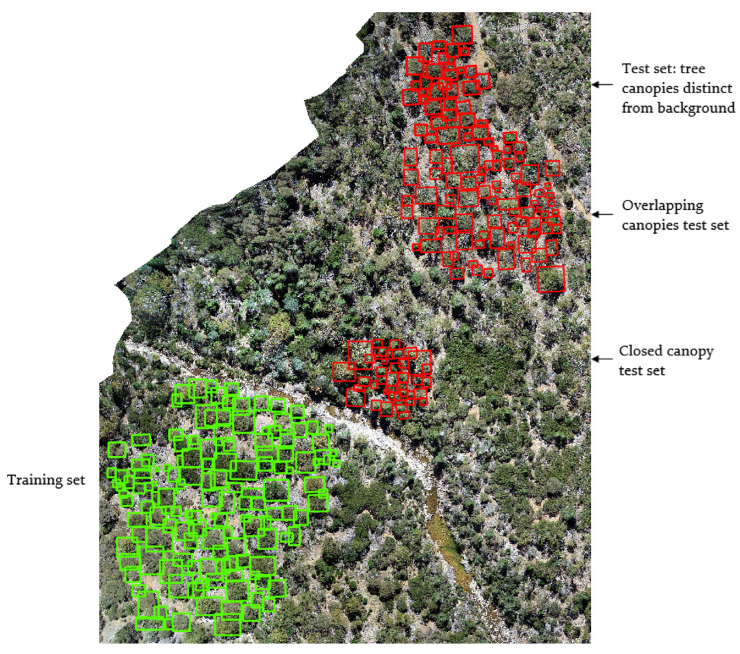
Figure 3. Location of the training (green) and three test (red) datasets. The training and test files were trimmed to include the extent of the bounding boxes.
Remotesensing 14 04963 g003
Figure 4. MRS results across different subsets. (A) Canopies with a distinct treetop crown structure and with gaps around trees were delineated without excessive oversegmentation or mixing between different classes. (B) In overlapping, dense canopies of similar height, there was undersegmentation where different species were represented in a single object. Branching Eucalyptus canopies were oversegmented in all subsets. (C) Results for the subset shown in Figure 1. Callitris rhomboidea crown and Eucalyptus pulchella branches erroneously combined in a segment.
Remotesensing 14 04963 g004
Figure 5. Superpixel segmentation results in a mixed canopy subset visualised using NIR, Red Edge and Blue bands (A). Region size is the average size of a superpixel. (B) Default value of 10 maintained image boundaries but oversegmented the image. (C) Average size of 35 pixels reduced oversegmentation. (D) Increasing Region Size beyond 35 resulted in reduced oversegmentation and superpixels representing individual tree canopies (i). However, in most areas, sizes over 35 caused undersegmentation. Different classes were grouped within a superpixel, for example, ground and canopies (ii) and overlapping canopies of different tree species Eucalyptus spp. and Acacia mearnsii canopies (iii).
Remotesensing 14 04963 g005
Figure 7. Feature and Permutation Importance at superpixel scale with Euc spp. aggregated. Features relevant were the same in both approaches (VIs and CHM). Based on random permutation of features, fewer features were relevant for the model.
Remotesensing 14 04963 g007
Figure 8. Classification map using superpixels. Inset shows classification in a Pulchella dominated forest subset. While the highest classification accuracy was achieved with superpixels, speckle effect is evident across the site at this scale. For example, canopy edges and shadow areas are misclassified as other species.
Remotesensing 14 04963 g008
Figure 9. Classification map using MRS objects. Pulchella dominated forest subset shown in inset. Speckle effect less prevalent at a coarser scale of analysis than superpixels.
Remotesensing 14 04963 g009
Figure 10. Classification map using DeepForest bounding boxes. Pulchella dominated forest subset shown in inset. Canopy edges falsely detected as individual trees.
Remotesensing 14 04963 g010
Figure 11. Predicted class and Confusion Index at the superpixel (A) and object (B) scales. Although classification accuracies were high (0.84 with superpixel, 0.77 at object scale), the Confusion Index was high, indicating high uncertainty in the predictions. This low confidence was not specific to a particular class or to locations in the canopies. This uncertainty is likely due to the spectral similarity between the tree species, and perhaps highlights the need for additional reference data, or input features to improve confidence in the predictions.
Remotesensing 14 04963 g011
Table 3. Accuracies of the pre-built model and model trained with tree bounding boxes from the study. Training the pre-built model with a small subset drastically improved accuracies.
DeepForest ModelPatch Size
(Pixels)
Training Accuracy
mAP
Test Accuracy
mAP
Closed Canopy and Trees Distinct from Background Dense, Closed Canopy
Subset
Overlapping Canopy Subset
Pre-built400N/A0.040.030.02
Trained10000.820.650.510.5
Table 4. OOB training and test accuracies with all 7 classes using the two different sets of spectra.
Scale of AnalysisInput FeaturesOOB Training AccuracyTest Accuracy
Spectra from All Pixels within Tree CanopySpectra from Pixels with SR Greater than Average Spectra from All Pixels within Tree CanopySpectra from Pixels with SR Greater than Average
SuperpixelSpectral, CHM0.770.810.790.83
Object0.700.730.710.74
Bounding box0.630.710.630.65
Table 5. Classification accuracies using spectral and incremental addition of Texture, Shape, and PPC features (when applicable). Input features and highest classification accuracy at each scale are in bold. Classification with Eucalyptus (Euc) spp. grouped in a class was performed with these input features.
Scale of AnalysisInput FeaturesClassesOOB Training AccuracyTest Accuracy
SuperpixelSpectral, CHMAll0.810.83
Spectral, CHM, TextureAll0.80.84
Spectral, CHM, TextureEuc spp. grouped0.880.93
ObjectSpectral, CHMAll0.730.74
Spectral, CHM, TextureAll0.740.77
Spectral, CHM, PPCAll0.710.71
Spectral, CHM, ShapeAll0.710.75
Spectral, CHM, Texture, PPC, ShapeAll0.710.75
Spectral, CHM, TextureEuc spp. grouped0.80.77
Bounding boxSpectral, CHMAll0.710.65
Spectral, CHM, TextureAll0.690.67
Spectral, CHM, PPCAll0.680.65
Spectral, CHM, Texture, PPCAll0.690.69
Spectral, CHM, Texture, PPCEuc spp. grouped0.760.77
Table 6. Class-specific accuracies: Precision, Recall, and F-score at the three scales of analysis.
ClassSuperpixelObjectBounding Box
PrecisionRecallF-ScorePrecisionRecallF-ScorePrecisionRecallF-Score
Acacia mearnsii10.830.910.50.50.50.60.60.6
Allocasuarina spp.0.8110.90.670.670.670.860.60.71
Callitris rhomboidea0.860.960.910.890.760.820.830.830.83
Eucalyptus pulchella0.790.730.760.770.940.850.580.850.69
Eucalyptus viminalis0.60.550.570.790.790.790.50.250.33
F-Score0.830.770.69
Table 7. Class-specific accuracies: Precision, Recall and F-score with grouped Eucalyptus species.
ClassSuperpixelObjectBounding Box
PrecisionRecallF-ScorePrecisionRecallF-ScorePrecisionRecallF-Score
Acacia mearnsii10.830.910.430.380.40.750.60.67
Allocasuarina spp.0.9210.9610.50.670.880.70.78
Callitris rhomboidea0.890.960.920.890.760.820.850.920.88
Eucalyptus spp.0.930.970.950.730.940.820.750.830.79
F-Score0.930.770.76
Table 8. Features important in the best performing model (Euc spp. aggregated) at each scale. Features listed had a permutation importance greater than 0 on the training set.
Scale of AnalysisImportant Features
(Based on Permutating Features)
OOB Training AccuracyTest Accuracy
SuperpixelNRBI, SR, r_rededge, CHM, NDVI0.880.93
ObjectNRBI, RBNDVI, CHM, NGBI, r_rededge, CIRE0.80.77
Bounding boxNRBI, CHM, M3CI, r_rededge, PSRI0.760.77
Publisher’s Note: MDPI stays neutral with regard to jurisdictional claims in published maps and institutional affiliations.