MAEANet: Multiscale Attention and Edge-Aware Siamese Network for Building Change Detection in High-Resolution Remote Sensing Images

Abstract

In recent years, using deep learning for large area building change detection has proven to be very efficient. However, the current methods for pixel-wise building change detection still have some limitations, such as a lack of robustness to false-positive changes and confusion about the boundary of dense buildings. To address these problems, a novel deep learning method called multiscale attention and edge-aware Siamese network (MAEANet) is proposed. The principal idea is to integrate both multiscale discriminative and edge structure information to improve the quality of prediction results. To effectively extract multiscale discriminative features, we design a contour channel attention module (CCAM) that highlights the edge of the changed region and combine it with the classical convolutional block attention module (CBAM) to construct multiscale attention (MA) module, which mainly contains channel, spatial and contour attention mechanisms. Meanwhile, to consider the structure information of buildings, we introduce the edge-aware (EA) module, which combines discriminative features with edge structure features to alleviate edge confusion in dense buildings. We conducted the experiments using LEVIR-CD and BCDD datasets. The proposed MA and EA modules can improve the F1-Score of the basic architecture by 1.13% on the LEVIR CD and by 1.39% on the BCDD with an accepted computation overhead. The experimental results demonstrate that the proposed MAEANet is effective and outperforms other state-of-the-art methods concerning metrics and visualization.

1. Introduction

Building change detection (BCD) is the procedure of extracting the dynamic changes in buildings in the same area based on remote sensing images acquired at different times. This process is of great importance to many fields, such as land resource utilization [1], urban expansion [2] and illegal construction management [3,4]. As more and more high-quality sensors are launched (e.g., IKONOS, QuickBird, GeoEye-1), many remote sensing images become accessible, which extensively drives the development of intelligent change detection technology. Concurrently, high-resolution remote sensing images, with their rich color information, clear textures and regular geometric structures [5], have become the primary data source for BCD.

As a hot issue in remote sensing image interpretation, change detection (CD) has been studied for several decades. The traditional CD methods can be categorized as follows: (1) image algebra, (2) image transformation and (3) machine learning methods [6]. The process of image algebra-based methods entail directly applying the spectral information difference or change vector analysis (CVA) [7] of bi-temporal images to obtain a feature difference map containing the magnitude of change. The final predicted map is obtained by clustering or threshold segmentation. Distinct from the image algebra-based methods, image transformation-based methods aim to extract more useful change information, such as histogram trend similarity [8] and principal component analysis (PCA) [9] and so on. However, despite simple theory and efficient performance, these methods still suffer from salt-and-pepper noise and poor promotion due to the lack of spatial context information or self-adaptive thresholds. To untangle these problems, machine learning algorithms, such as decision trees [10], random forests [11,12] and support vector machines [13], are designed based on thresholding operator. In addition, spatial context information is introduced by Markov random field [14] and Conditional random field [15] to reduce the noise influence. Based on these methods, the automation of CD has been significantly improved. However, the features used by the CD algorithm are artificially selected, so they have a poor image representation and exhibit weak robustness.

Recently, powered by tremendous machine learning, deep learning methods have achieved extraordinary achievements in the fields of object detection [16,17], image classification [18], and CD [19,20] with their excellent learning capabilities and robust adaptability. In contrast to traditional features, deep features generated based on convolutional neural networks (CNNs) effectively integrate abstract and conceptual high-level information from bi-temporal satellite images and significantly distinguish between changed and unchanged features. In general, deep learning methods for BCD contain two primary methods: (1) post-classification based and (2) direct-detection based methods [21]. Normally, the former extract buildings from different phase images independently, and the final building change map is generated by analyzing their differences. Although it can easily handle multi-model and multi-sensor images, it highly depends on the multi-temporal image registration and classification performance. The latter adopts the end-to-end framework that effectively overcomes the problem of insufficient semantic information due to manual design features and is currently the mainstream approach for CD [22]. Generally, the direct-detection-based methods can be simplified into two steps: (1) extracting discriminative features, and (2) designing a decision process that can generate a predicted map according to the extracted features [23,24].

Considering the problems of geometric misregistration and spectral difference caused by factors such as illumination, noise and biological seasonality in the bi-temporal image, mining more discriminative features with contextual information is an excellent way to improve the CD accuracy as well as improve the robustness of the model to different scenes. In [25], Chen and Shi proposed a STANet with a self-attentive mechanism, aiming to construct a CD network based on the spatio-temporal relationships between different times and locations of bi-temporal images. In [26], Mou et al. propose a ReCNN architecture for bi-temporal multispectral remote sensing image analysis. Recurrent neural networks (RNNs) are used to introduce temporal information to the network because they can easily capture temporal dependence between multitemporal images. In [27], Chen et al. designed SiamCRNN, combining convolutional and recurrent neural networks into one framework. Both spectral-spatial information and temporal dependence are considered for multispectral image change detection.

Furthermore, the process aims to generate a predicted map that plays a vital role in change detection. The classification-based architecture, mainly based on the FCN structure, has been widely used in CD [28,29,30]. Compared with metric-based architecture, which determines the change by measuring the parameterized distance between the features, classification-based architecture obtains the change map by calculating the change score for each pixel. For changed pixels, a high score will be assigned, and for unchanged pixels, a low score will be assigned. The classification-based architecture enables the CD task to be viewed as a classification task, and its powerful nonlinear classification capability can significantly improve the robustness of the CD.

Despite the remarkable achievements of deep learning methods [31,32], existing CD methods still have some challenges. Several current studies have shown that introducing temporal dependence can effectively improve the differentiation of features [24,33]. However, the false-positive changes caused by shadow and complex appearance are still hard to distinguish based on temporal information. Therefore, exploring effective techniques to extract discriminatory information and mitigate the false-positive changes is worthwhile. Meanwhile, the deep semantic information often lacks detailed boundary information, resulting in poor boundary integrity of detected change objects and boundary confusion in dense buildings. Thus, it is a vital challenge to recover the morphology of the changed objects.

To solve the issues of false-positive changes and boundary confusion in bi-temporal images dense BCD, a novel end-to-end multiscale attention and edge-aware network (MAEANet) is proposed in this article. Among them, we design two modules to improve the change detection performance of the network. Concerning enhancing the discrimination of features, we introduce a multiscale attention (MA) module, which mainly consists of the convolutional block attention module (CBAM) [34] and a contour channel attention module (CCAM). Meanwhile, we introduce an edge-aware (EA) module in the last two layers to reduce the confusion between dense buildings.

The main contributions of this article are as follows:

(1) In this article, a novel network called MAEANet is proposed for BCD. Both discriminative and prior edge information are combined into one framework to enhance the quality of binary BCD results.

(2) We focus on two aspects to improve the performance of BCD networks, respectively. In terms of enhancing the discriminability of features, we proposed a MA module, including the classical CBAM module and a CCAM module designed to be able to highlight the edge of changed objects. The CBAM is used in deep features with more semantic information, while CCAM is more concerned with recovering boundary information. In terms of improving the quality of building boundary, we introduced an EA module that can better maintain the building boundary while generating binary change detection results, which can successfully overcome the boundary confusion problem of buildings.

(3) The results of a series of experiments show that the proposed MAEANet outperforms other state-of-the-art methods in metrics such as F1-Score and Kappa Coefficient on remote sensing image BCD datasets. Meanwhile, the advantage is that it does not need post-processing to obtain better pixel-level binary prediction maps.

The remainder of this article is organized as follows: we describe the detailed network composition parts in Section 2. Then, the experimental results and their visualization are presented in Section 3. Next, building edge performance comparison and some parameterization setting experiments are discussed in Section 4. Finally, Section 5 presents a summary of the proposed method.

2. Methods

In this section, we further describe the detailed information about the MAEANet network. Then, the specific information on Siam-fusedNet network (Siam-fusedNet), MA module and EA module is introduced. Finally, we further explain the principle of the hybrid loss function used for BCD.

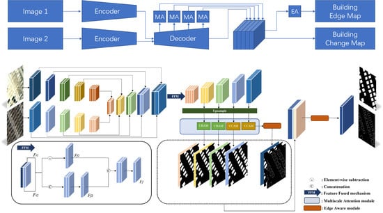
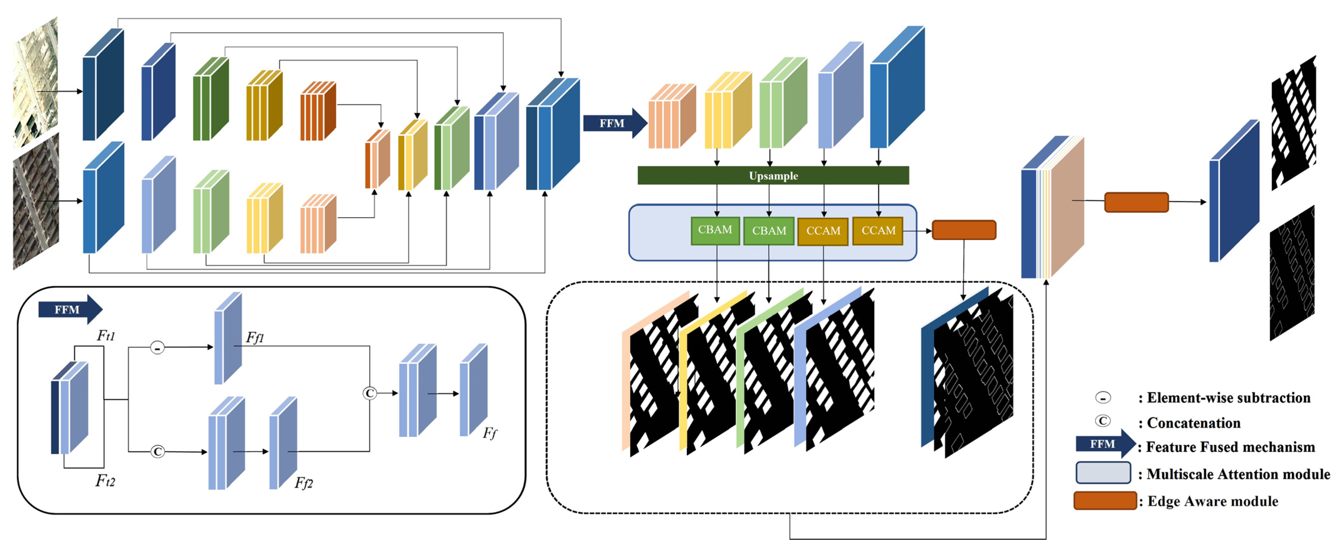
2.1. Overview of MAEANet Network

The proposed MAEANet network mainly consists of three parts: the base architecture of the Siam-fusedNet, the MA module and the EA module. The first step of MAEANet is to crop the bi-temporal images into 256 × 256 and feed them into Siam-fusedNet to extract the initial features. Then, the MA module is added to extract discriminative information from the multiscale features after upsampling. The final binary predicted map is generated by adding a multilevel EA module that effectively introduces the edge information. More specific descriptions are shown in Figure 1.

2.2. Siam-fusedNet

We adopt the Siamese network as the basic reference to design the bi-temporal BCD network. In terms of feature extraction, since the binary BCD task can be seen as a classical semantic segmentation task, UNet [35] with an encoder-decoder structure is utilized to obtain abundant multiscale features. Meanwhile, to exploit as much helpful information as possible, a bi-temporal feature fused mechanism (FFM) is added after UNet. Here is the detailed workflow of Siam-fusedNet.

The bi-temporal images are fed into the network independently. First, the encoder of the network has two streams with shared weights and the pre-trained module of ResNet34 [36] is introduced. Then, in the decoder, we use upsampling to recover the image’s resolution and adopt skip-connection to combine the underlying location information with the deep semantic information to recover the edge detail information lost during the encoding process.

To improve the learning of parallel feature differences between two-branch decoders in the same scale layer, a bi-temporal FFM [37] is used. As shown in the bottom left part of Figure 1, it consists of two branches: the difference and the concatenation. Firstly, we take the parallel features $F_{t1}$ and $F_{t2}$ from the same scale layer as the input. Then, in the concatenation branch, for the adaptive acquisition of local features critical to change, fusion features $F_{t1}$ are generated by parallel features between $F_{t1}$ and $F_{t2}$. Finally, the fused features $F_{t1}$ and $F_{t2}$ learned from two distinct branches are integrated and then processed through the Batch normalization (BN) and LeakyReLU operations to obtain the eventually fused feature $F_f$. The detailed calculation formulas are as follows:

$$F_{f1}=F_{t1}-F_{t2}$$

(1)

$$F_{f2}=Con{v}_{1\times 1}\left(Concat\left(F_{t1},F_{t2}\right)\right)$$

(2)

$$F_f=LeakyReLU\left(BN\left(Con{v}_{1\times 1}\left(F_{f1},F_{f2}\right)\right)\right)$$

(3)

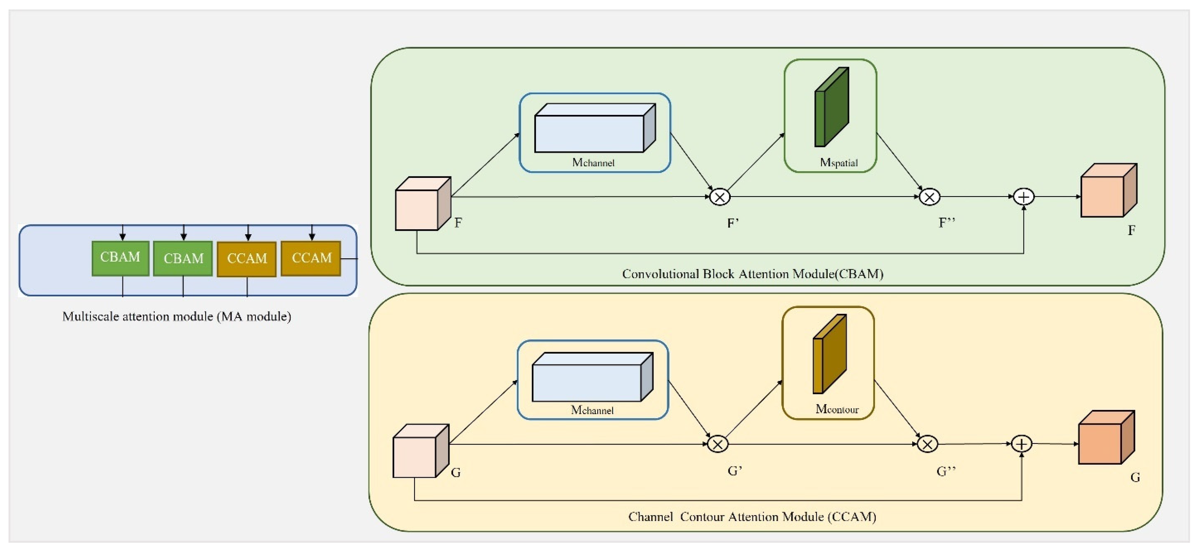
2.3. Multiscale Attention (MA) Module

One of the most critical issues in the feature extraction process is compressing the information of irrelevant features and better highlighting the information of changed features. Therefore, the MA module is designed in this paper. The MA module covers three kinds of attention mechanisms: channel, spatial and contour attention mechanisms, and its main component models are CBAM and CCAM.

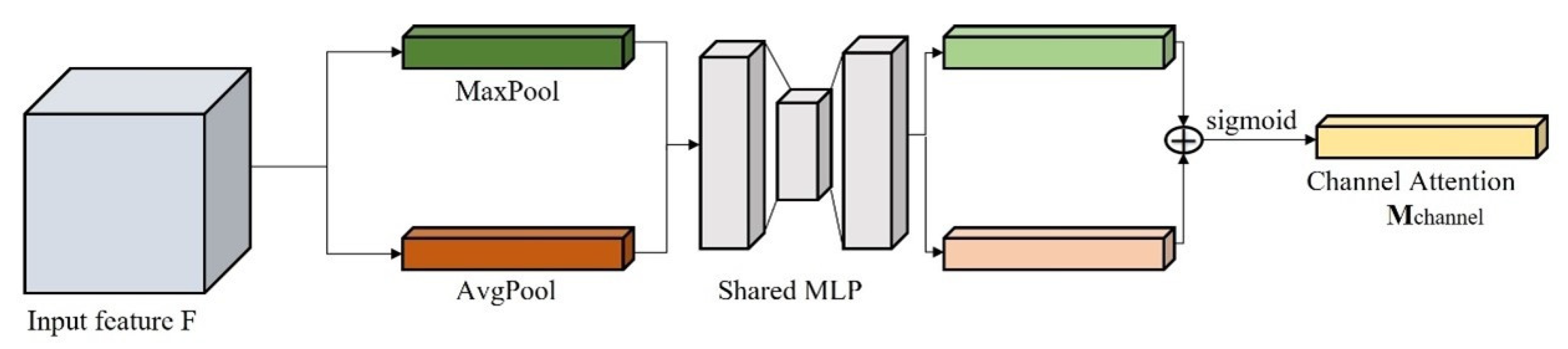
2.3.1. Channel Attention Mechanism

The channel attention mechanism focuses on “what” benefits the original image [34]. Therefore, we commonly use the method of computing channel attention maps to acquire the inter-channel relationships of features. For example, feature channels associated strongly with change detection will be emphasized, while feature channels unassociated strongly with change detection will be suppressed. Figure 2 shows the detailed structure of the channel attention mechanism and the formula of the channel attention map ($M_{channel}$) is calculated as follows:

$$M_{channel}=\sigma \left(MLP\left(MaxPool\left(F\right)\right)+MLP\left(AvgPool\left(F\right)\right)\right)$$

(4)

where $F$ denotes the original feature of size $C\times H\times W$. Firstly, we calculate the input features’ max pooling and average pooling separately to generate two $C\times 1\times 1$ aggregation vectors. Then, two $C\times 1\times 1$ aggregation vectors are input into a weight-shared multilayer perception (MLP) layer, which mainly consists of reducing the number of channels to $r$ and recovering them. Finally, an element-wise sum is adopted for two types of vectors and a nonlinear operation is used to obtain the final channel attention map.

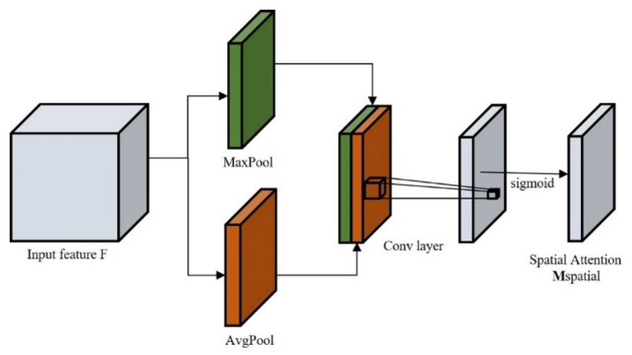
2.3.2. Spatial Attention Mechanism

The spatial attention mechanism concentrate on “where” is helpful to the input image. Therefore, a spatial attention map is computed to capture the location relationship of features. For example, locations in the features consistent with changed pixels will be given higher weights, while inconsistent locations will be given lower weights. The spatial attention mechanism is shown in Figure 3 and the formula of the spatial attention map ($M_{spatial}$) is calculated as follows:

$$M_{spatial}\left(F\right)=\sigma \left(f^{\left(k\times k\right)}\left(\left[AvgPool\left(F\right);MaxPool\left(F\right)\right]\right)\right)$$

(5)

where $F$ denotes the original feature of size C × H × W. Firstly, we calculate the input features’ max pooling and average pooling separately to generate 1 × H × W aggregation vectors. Then, two vectors are concatenated, and a Conv operation is applied with a kernel size of 7 × 7 to generate a highlighting feature of size 1 × H × W. Finally, a nonlinear operation is used to obtain spatial attention map.

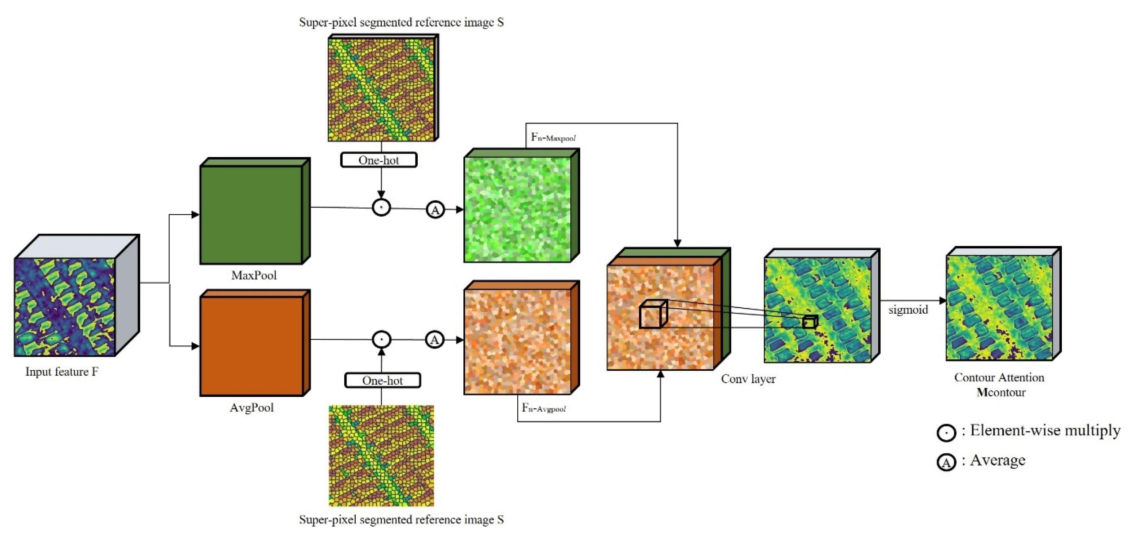
2.3.3. Contour Attention Mechanism

The contour attention mechanism is more concerned with the internal consistency of the changed objects. Therefore, a contour attention map that introduces the super-pixel objects is calculated to ensure the pixels within an object only own one category, either changed or unchanged. The internal pixel consistency will be enhanced for changed objects and weakened for unchanged objects. As a result, compared with the original pixel-wise, super-pixel objects have superior performance in presenting the local structural information of the image.

In comparison with various super-pixel generation methods proposed so far, Simple Linear Iterative Clustering (SLIC) [38] is an effective algorithm with comparative performance in terms of metrics such as under-segmentation error, boundary recall and explained variance [39]. Meanwhile, it also has outstanding advantages in boundary preserving. The SLIC aims to build region clusters based on the k-means algorithm with seed pixels initialization. Each pixel on the image is described as a five-dimensional feature vector ${\left[l,a,b,x,y\right]}^T$. The parameter to be customized is $K$, which indicates the number of super-pixel objects expected to be generated. The optional parameter $m$ represents the compactness of the super-pixel objects. After comparing several different sets of experiments, we find that the best segmentation results are obtained when we set the value of 𝐾 to 900 and the value of 𝑚 to 30. The specific process of super-pixel segmentation can be divided into three steps:

(1) Divide the image uniformly according to the number of segmented objects and calculate the interval size;

(2) Adopt the location with the smallest gradient in the 3 × 3 neighborhoods of the cluster center as the new cluster center to avoid placing seeds on edges or noisy pixels [38,40];

(3) Through a multiple iteration process, disjoint pixels are assigned to nearby super-pixel based on the distance measure $D$. Typically, the number of iterations will be set to 10. The formula for calculating the distance $D$ is as follows:

$$d_c=\sqrt{{\left(l_i-l_j\right)}^2+{\left(a_i-a_j\right)}^2+{\left(b_i-b_j\right)}^2}$$

(6)

$$d_s=\sqrt{{\left(x_i-x_j\right)}^2+{\left(y_i-y_j\right)}^2}$$

(7)

$$D=\sqrt{{\left(\frac{d_c}{m}\right)}^2+{\left(\frac{d_s}{S}\right)}^2}$$

(8)

where $\left(x_i,y_i\right)$ represents the location of pixel $i$ and $\left(l_i,a_i,b_i\right)$ represents the color component of pixel $i$ in the CIELAB color space [41]. $d_c$ and $d_s$ denote the color proximity distance and spatial proximity distance, respectively.

As shown in Figure 4, the framework of the contour attention mechanism has two inputs, the original feature $F$ and the super-pixel segmented reference image $S$. The super-pixel segmentation map $S$ after one-hot processing will be used as the guide image for subsequent original feature extraction. In this way, we aim to describe the internal consistency information more closely, especially for complex and diverse buildings. The formula of contour attention ($M_{contour}$) is calculated as follows:

$$P=S_{one-hot}·Pool\left(F\right)$$

(9)

$$w=\frac{{\sum }_{i=1}^n{\sum }_{j=1}^{m}P}{{\sum }_{i=1}^n{\sum }_{j=1}^{m}S}$$

(10)

$$F_n=reshape\left({{\displaystyle \sum }}_{j=1}^m\left(S_{one-hot}·w\right)\right)$$

(11)

$$M_{contour}\left(F\right)=\sigma \left(f^{\left(k\times k\right)}\left(\left[F_{n-MaxPool};F_{n-AvgPool}\right]\right)\right)$$

(12)

where $F$ represents the original image feature and $S$ represents the super-pixel segmented post-temporal image. Firstly, we compute the max pooling and avg pooling of the original features separately. Meanwhile, the one-hot processed super-pixel segmentation image is produced and multiplied with the pooled feature to obtain $P$. The number of segmented objects is $n$, and $m$ is the total number of pixels. Calculated $P$ contains the original feature information and the index information of the super-pixel segmented objects. Then, we calculated the $w$ to describe the average of the original feature in super-pixel segmented objects. Furthermore, we multiply $w$ with the one-hot processed super-pixel segmentation image to generate the new feature $F_n$. Finally, we concatenate two new features generated by averaging and pooling features to obtain more channels to feature. Meanwhile, a Conv operation with the kernel size of 7 × 7 and a nonlinear operation are adopted to obtain the final contour attention map ($M_{contour}$).

The structure of the MA module mainly contains two parts: CBAM [34] and the proposed CCAM module, respectively. The detailed description is shown in Figure 5. CBAM focuses on the changed information and is composed of the channel and spatial attention mechanisms. CCAM integrates information about changed objects and comprises channel and contour attention mechanisms. In the proposed MAEANet network, we introduce CBAM after deep features with more semantic information and CCAM after shallow features with more detailed location information. The formula of CBAM and CCAM is calculated as follows:

For CBAM:

$$F^{\prime }=M_{channel}\left(F\right)\times F$$

(13)

$$F^{″}=M_{spatial}\left(F^{\prime }\right)\times F^{\prime }$$

(14)

$$F=F^{″}+F$$

(15)

For CCAM:

$$G^{\prime }=M_{channel}\left(G\right)\times G$$

(16)

$$G^{″}=M_{contour}\left(G^{\prime }\right)\times G^{\prime }$$

(17)

$$G=G^{″}+G$$

(18)

where $F$ represents the deep feature and $G$ represents the shallow feature. After introducing the $M_{channel}$, $M_{spatial}$ and $M_{contour}$ to CBAM and CCAM successively, more discriminative features about $F$ and $G$ are acquired.

Figure 5. The internal components of the MA module.

Figure 5. The internal components of the MA module.

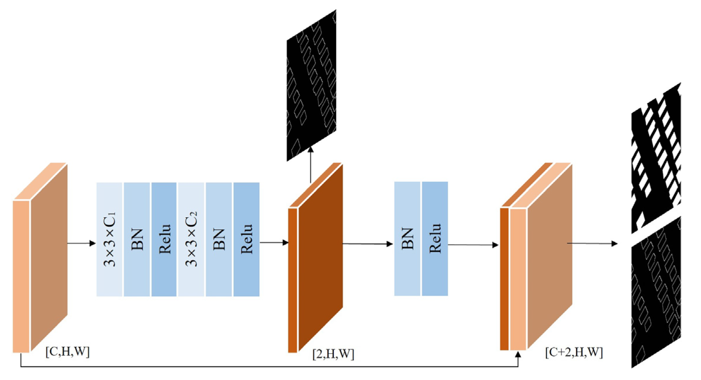
2.4. Edge Aware Module

Recent studies have shown that introducing the building edge information in deep supervision can effectively generate better quality BCD results [32,42]. The main reason is that the edge information of buildings has a distinct geometric structure, which is very effective for determining the location of buildings. At the same time, adequate edge information can guide the network to generate better binary prediction results, especially in dense building areas. Based on the above considerations, we introduce the EA module to MAEANet.

As shown in Figure 6, we combine our module’s edge estimation task and building change prediction task to achieve a mutually reinforcing effect. Firstly, we use the Conv block, which includes a convolution kernel with the size of 3 × 3, BN and Relu to extract edge information. The $C_1$ represents the channel number of the original feature and $C_2$ is set to 2. After the above operation, we obtain the edge information from the output. Then, we adopt the BN and Relu to further obtain nonlinear boundary information. Finally, original features are concatenated with edge information to estimate the binary change and edge prediction maps. The advantage of the EA module is that the edge feature can be integrated directly into the discriminant feature, thus improving the accuracy of detecting building changes and alleviating the mixing and misclassification of building edges.

2.5. Loss Function Details

To achieve training and optimization of the network, we design a deep hybrid loss function which not only includes a loss function that tends to focus on change detection ($E_{wbce}$) but also a loss function that focuses on edge detection ($E_{Dice}$). Since the unchanged sample counts are much higher than the changed sample counts in the actual change detection task, we introduce a weighted binary cross-entropy loss to modify the imbalance training samples. The specific binary cross-entropy loss can be described as:

$$E_{wbce}=\frac{1}{N}\times \left[\omega {\displaystyle \sum }_{y_n=1}{y}_n\times \log \left(p_n\right)+\left(1-\omega \right){\displaystyle \sum }_{y_n=0}\left(1-y_n\right)\times \log \left(1-p_n\right)\right]$$

(19)

where $N$ is the total pixel count of the image; $\omega$ is defined to reduce the weight of negative samples and increase the focus on positive samples during the training process of the network; $y_n$ is the n-th sample pixel, when $y_n$ = 0 means that the pixel is unchanged, while $y_n$ = 1 denotes the changed pixel. $p_n$ is the expression of the probability of change.

In addition, the dice coefficient loss can weaken the category imbalance and work well in change detection tasks. Therefore, we adopt the dice coefficient loss to describe the edge detection. The formula for dice coefficients loss is expressed as:

$$E_{dice}=1-\frac{2\gamma \widehat{\gamma }}{\gamma +\widehat{\gamma }}$$

(20)

where $\gamma$ denotes the predicted probability value of all change class pixels in the image, and $\widehat{\gamma }$ denotes the ground truth value of the image.

The final hybrid loss function can be calculated as follows:

$$E=E_{wbce}+\lambda E_{dice}$$

(21)

where the weight ratio λ is used to balance the influence of change detection and edge detection, we set it to 10. Through the continuous training of the hybrid loss, the eventually obtained building change results will present more accurate bounds while maintaining higher accuracy.

3. Experiments and Results

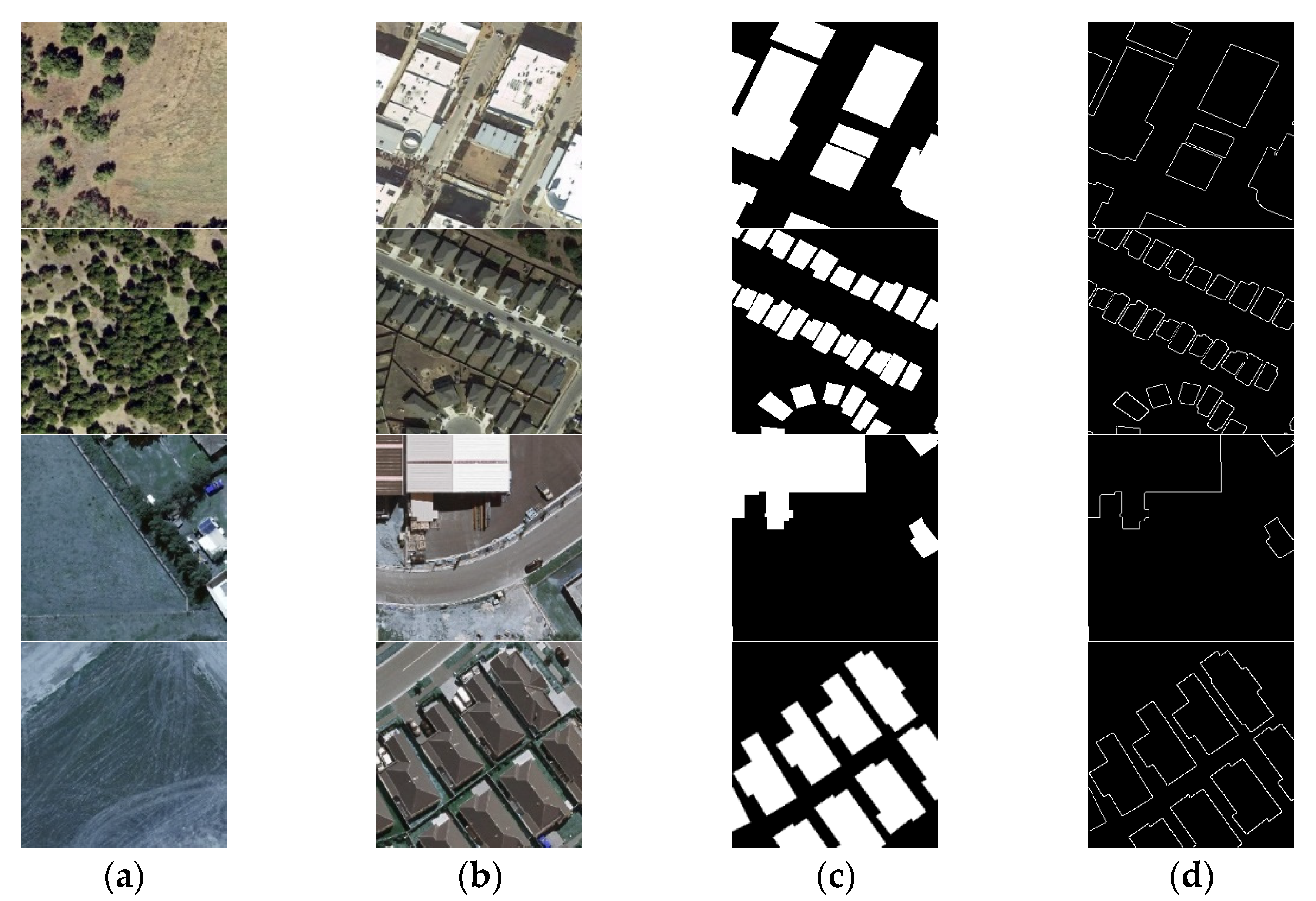
3.1. Data Description

To prove the validity of MAEANet, we conduct experiments on two publicly available datasets: LEarning VIsion Remote Sensing (LEVIR CD) [25] and WHU Building Change Detection Dataset (BCDD) [30]. Figure 7 shows some images obtained from LEVIR CD and BCDD.

LEVIR CD dataset is a public, large-scale CD dataset with a total of 637 pairs of images. The dataset is a 3-band multi-temporal image with a 0.5 m spatial resolution. The images covering building changes vary from 2002 to 2018 in 20 regions of Texas, USA. In addition, some influencing factors such as illumination and seasonal changes are considered, which help us in developing more robust methods. Taking into account the limited memory of our GPU, we chose to crop the image to 256 × 256 pixels without overlap. Furthermore, since the changed building instances account for a relatively small amount of the whole dataset, some data augmentation operations, such as random rotation, are used. Finally, we obtain 8256/1024/2048 pairs of images to generate training, validation, and test set.

WHU Building Change Detection Dataset (BCDD) is a public dataset containing two scenes of aerial data acquired in Christchurch, New Zealand, in 2012 and 2016. This bi-temporal dataset is 32,507 × 15,354 pixels in size with a total of 11,328 pairs of images and has a 1.6 m spatial resolution. In addition, we crop each image into the patch of size 256 × 256 pixels without overlap, obtaining 7434 image pairs. Finally, we obtain 5204/744/1486 pairs of images for training, validation and test.

3.2. Comparison Methods

We selected four deep learning-based CD methods to objectively evaluate the performance of the MAEANet, as described in below.

MSPSNet [22] is a deeply supervised multiscale Siamese network. The network learns effective feature maps through the convolutional block. Furthermore, it integrates feature maps by parallel convolutional structure, while self-attention further enhances the CD representation of image information.

SNUNet [31] is proposed for CD based on densely connected Siamese networks. The network reduces the localization information loss during feature extraction through dense connections between encoders and decoders. In addition, the Ensemble Channel Attention is introduced to advanced representation features at different semantic levels.

STANet [25] is a metric-based Siamese neural network that identifies bi-temporal image CD. The network feeds ResNet18 as a backbone, introduces the self-attention to build the temporal and spatial relationship, and then uses it to capture various scales of spatial-temporal dependencies at multiscale subregions.

EGRCNN [32] uses the convolutional neural network for BCD. The network feeds bi-temporal images into a weight-shared Siamese network for extracting primary multilevel features. It then provides a long short-term memory (LSTM) module to produce the feature. In addition, the edge structure of the building is introduced into the network, aiming to improve the BCD’s quality.

3.3. Implementation Details and Evaluation Metrics

In this article, all of the experiments were implemented based on the Pytorch framework, and the network was conducted on a single Nvidia Tesla V100 (16 GB of RAM). We performed data augmentation on the training data, such as rotation and flipping. During training, we used the Adam optimizer with an initial learning rate of 10⁻⁴ and the learning rate decay strategy was also used. The batch size was set to be 4 and the epoch was 100. If the F1-score did not increase after 15 epochs, we would reduce the learning rate by 10 times. The parameter ω in the $E_{wbce}$ was set to be 0.25. The comparison methods were the same as the public code and all parameter settings were the default parameters of the original papers.

To quantitatively verify the performance of the network, five general used metrics were used: Precision (P), Recall (R), F1-score (F1), Overall Accuracy (OA), and Kappa Coefficient (KC). The P is the proportion of correctly detected changed pixels to all identified changed pixels. The closer the value of P to 1, the lower the error detection rate of the predicted value. The R is the proportion of correctly detected changed pixels relative to all pixels that should be recognized as changed. The closer the R value is to 1, the lower the rate of missed detections of predicted values. The F1 is the harmonic average of P and R. When one of them decreases, the F1 also decreases. The OA indicates the ratio of correctly detected change pixels in all samples. The KC represents the similarity between the predicted map and the ground truth. The equations of these evaluation metrics are as follows:

$$P=\frac{TP}{TP+FP}$$

(22)

$$R=\frac{TP}{TP+FN}$$

(23)

$$F1=\frac{2PR}{P+R}$$

(24)

$$OA=\frac{TP+TN}{TP+TN+FP+FN}$$

(25)

$$P_e=\frac{\left(FP+TP\right)\left(FN+TP\right)+\left(TN+FN\right)\left(TN+FP\right)}{{\left(TP+TN+FP+FN\right)}^2}$$

(26)

$$KC=\frac{OA-P_e}{1-P_e}$$

(27)

where TP, FP, TN, and FN represent the correctly classified true positive count, the correctly classified false positive count, the correctly classified true negative count, and the correctly classified false negative count, respectively.

3.4. Ablation Study for the Proposed MAEANet

To prove the efficiency of each component in MAEANet, a series of ablation experiments are conducted for the MA and EA module using the LEVIR CD and BCDD dataset. In detail, we adopt the Siam-fusedNet as the base architecture to extract original features. The MA module is introduced to enhance the discrimination of original features and refine the misclassification. Introducing the EA module aims to improve the boundary quality of dense buildings. Detailed experiments are shown in

Table 1. The ablation experiment results in LEVIR CD and BCDD adding MA and EA modules.

	Methods	MA	EA	Precision (%)	Recall (%)	F1-Score (%)	OA (%)	KC (%)
LEVIR CD	Siam-fusedNet	×	×	85.80	91.95	88.77	88.15	98.81
	MAEANet	√	×	89.36	90.24	89.80	89.25	98.95
	MAEANet	×	√	89.43	89.48	89.45	88.89	98.93
	MAEANet	√	√	88.84	91.00	89.90	89.35	98.95
BCDD	Siam-fusedNet	×	×	94.02	86.66	90.19	99.28	89.81
	MAEANet	√	×	92.61	89.36	90.95	99.31	90.61
	MAEANet	×	√	93.31	88.74	90.96	99.32	90.62
	MAEANet	√	√	92.82	90.38	91.58	99.36	91.25

, and the most optimal results are highlighted in bold.

Considering the data of LEVIR CD in Table 1, the results of the Siam-fusedNet for P, R, F1, OA and KC are 85.80%, 91.95%, 88.77%, 88.15% and 98.81%. After adding the MA module, P, R, F1, OA and KC are 89.36%, 90.24%, 89.80%, 89.25%, and 98.95%, respectively, and metrics of P, F1, and OA are improved by 3.56%, 1.03%, and 1.1% compared with Siam-fusedNet. When the EA module is added, we obtain the P, R, F1, OA and KC are 89.43%, 89.48%, 89.45%, 88.89% and 98.93%. Compared to the Siam-fusedNet, the P, F1 and OA metrics of the network with the EA module improved by 3.63%, 0.68% and 0.74%. When MA and EA modules are added to Siam-fusedNet simultaneously, the highest values of 89.90%, 89.35% and 98.95% are achieved for F1, OA and KC, respectively.

Considering the data of BCDD in Table 1, the metrics of the Siam-fusedNet for P, R, F1, OA and KC are 94.02%, 86.66%, 90.19%, 99.28% and 89.81%. The value of P is satisfactory, but the value of R is poor, which means that the performance of Siam-fusedNet is unstable. To improve the metric value of R, we observe that the value of R after adding the MA module is nearly 2.7% higher than Siam-fusedNet and adding the EA module is almost 2.08% higher than Siam-fusedNet. When we add both the MA and EA module to the Siam-fusedNet, the network’s capability is greatly enhanced, with F1, OA and KC values of 91.58%, 99.36% and 91.25%. From the above experimental results, when we introduce the MA and EA module into the Siam-fusedNet, the difference between P and R is the smallest while the F1 is the highest, thus strongly verifying the performance of the MAEANet.

To further illustrate the method’s superiority in change detection, some visual comparisons of the results in the ablation experiment are conducted, as shown in Figure 8. As we can see, many false positives are classified as changes (rows 1 and 5 in Figure 8) and some changed buildings without clear boundaries (rows 3, 4, 6 and 7 in Figure 8) in the Siam-fusedNet model. The reason is that CD is affected by bi-temporal illumination, color and other factors. Therefore, the feature information in bi-temporal images cannot be extracted well using only the convolutional blocks in an ordinary Siam-fusedNet network. After adding the EA module to the Siam-fusedNet network, we find the edge of building visual effect is optimized to some extent (rows 1, 4 and 7 in Figure 8) because the EA module can better mine the boundary information of buildings. When we introduce the MA module to the Siam-fusedNet network, the problem of false positive changes has been significantly solved and the quality of the building boundaries has been further improved (rows 2, 3, 4, 5 and 6 in Figure 8). When the MA module and EA module are consistently added to the Siam-fusedNet, the misclassification change information is dramatically reduced, and the boundary between adjacent buildings is clear and closer to the ground truth value.

3.5. Comparison Experiments

To objectively and quantitatively compare our proposed MAEANet with existing CD methods, a series of comparison experiments are conducted on two datasets and three evaluation metrics are calculated for analysis, P, R and F1, respectively. Specific results are shown in

Table 2. The comparison experiments on the LEVIR CD and BCDD. (The best result is highlighted in bold.).

Method	LEVIR CD			BCDD
	Precision (%)	Recall (%)	F1-Score (%)	Precision (%)	Recall (%)	F1-Score (%)
MSPSNet [22]	88.74	87.44	88.09	75.84	78.59	77.19
SNUNet [31]	88.14	77.31	82.37	76.73	72.12	74.35
STANet [25]	81.30	89.90	85.40	81.90	85.90	83.80
EGRCNN [32]	86.43	89.87	88.11	90.74	88.92	89.82
MAEANet	88.84	91.00	89.90	92.82	90.38	91.58

.

By comparing the metric values in Table 2, it can be found that MAEANet obviously outperformed the other networks in P, R and F1 metrics. Although MSPSNet and SNUNet achieve promising accuracy values, more omissions exist for objects that have changed, resulting in lower values of R and F1. When we compare STANet with the proposed MAEANet, the P, R and F1 metrics of the MAEANet improved by 7.54%, 1.1% and 4.5% on the LEVIR CD dataset and by 10.9%, 4.48% and 7.78% on the BCDD dataset. The main reason is that our proposed attention module takes into account the internal consistency of objects, thus reducing misclassification due to bi-temporal differences. Compared to EGRCNN, the F1 of MAEANet is 1.79% and 1.76% higher than EGRCNN on the LEVIR CD and BCDD datasets, which proved its excellent performance in detecting changed buildings.

Simultaneously, the visual results between the proposed MAEANet and other methods are shown in Figure 9. By subjective visual comparison with the above-mentioned change detection methods, it can be found that the binary CD results are superior to the other existing methods. The comparison of the visible result in Figure 9 shows that for the dense building, MSPSNet, SNUNet and STANet have significant boundary confusion problems (rows 1, 3 and 4 in Figure 9). Still, the method of EGRCNN and our proposed MAEANet overcome this problem. The main reason is that both EGRCNN and MAEANet introduce the edge prior information, thus avoiding the problem of building boundary confusion. For the changed large-size individual houses, the proposed MAEANet is most reliable to other methods in maintaining the internal consistency of the building and the integrity of its boundaries (rows 2, 5 and 6 in Figure 9).

4. Discussion

4.1. Quantitative Comparison of Binary Edge Prediction Results

To compare the performance of the proposed MAEANet with the above-mentioned change detection methods in boundary maintenance, we generate the binary boundary learning results by performing morphological processing within a 9 × 9 neighborhood on the binary change detection images. Corresponding evaluation metrics are calculated, as shown in

Table 3. The results of boundary maintenance with different methods. (The best result is in bold).

	Precision (%)	Recall (%)	F1-Score (%)	OA (%)	KC (%)
MSPSNet	71.57 ± 2.54 (+16.5)	79.23 ± 0.11 (+8.54)	75.19 ± 1.39 (+12.73)	92.03 ± 0.40 (+4.29)	70.46 ± 1.10 (+15.29)
SNUNet	70.41 ± 2.37 (+17.66)	80.30 ± 0.19 (+7.47)	75.02 ± 1.28 (+12.9)	91.85 ± 0.41 (+4.47)	70.16 ± 0.93 (+15.59)
STANet	73.54 ± 2.32 (+14.53)	75.30 ± 0.69 (+12.47)	74.31 ± 0.90 (+13.61)	92.08 ± 0.52 (+4.24)	69.62 ± 0.50 (+16.13)
EGRCNN	84.51 ± 1.25 (+3.56)	86.50 ± 0.47 (+1.27)	85.49 ± 0.86 (+2.43)	95.53 ± 0.27 (+0.79)	82.84 ± 0.67 (+2.91)
MAEANet	88.07 ± 0.83	87.77 ± 0.11	87.92 ± 0.44	96.32 ± 0.30	85.75 ± 0.25

. We can see that the best results are obtained for P, R, F1, OA, and KC when MAEANet is used. Compared with three models that do not considering boundary factors, such as MSPSNet, SNUNet and STANet, all five metrics show significant improvements. We also find that MAEANet still maintains an excellent performance compared to EGRCNN with boundary factors, where the F1 improves by 2.01% and KC improves by 2.49%. Therefore, it is powerfully demonstrated that the proposed MAEANet has obvious superiority in the boundary maintenance of CD.

In our MAEANet method, the building edge information is mainly extracted by the contour attention mechanism with the SLIC over-segmentation operator. Alongside the edge information intuitively from the RGB images, extra information extracted from the corresponding digital surface models (DSMs) has been introduced into the building extraction tasks. It is obvious that the DSMs data can provide more edge information of the flat roofs of buildings without the influence of building shadows or the spectral confusion between buildings and roads. Intuitively, the introduction of DSMs data can yield performance gain in the building extraction tasks, as well as the building change detection tasks.

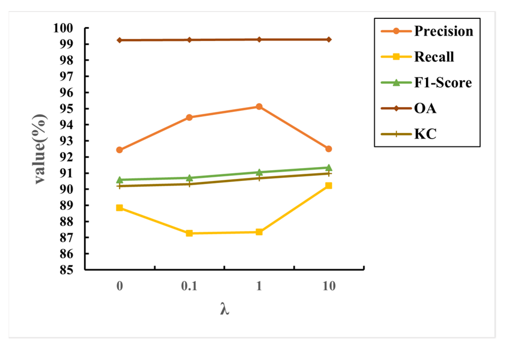
4.2. The Experiments on the Hybrid Loss

The weighted binary cross entropy loss focuses on image prediction and dice coefficient loss focus on edge map estimation. In the hybrid loss function proposed in this paper, we set a scale factor λ to balance the effects of the two different loss functions mentioned above. Meanwhile, to verify whether the edge-based dice coefficient loss is effective for the whole MAEANet, we set four scale factors, 0, 0.1, 1, and 10 [32], and conducted experiments on the BCDD dataset.

As shown in Figure 10, we calculate five different metrics for comparison and validation. When the parameter λ is 0, the performance in each metric is the lowest value. As the value of λ increases, the value of F1 and KC show steady growth, although the value of P tends to rise and then fall and the R tends to fall and then rise, which indicates that the introduced distance loss can improve the change detection effect of the building. In addition, we notice that when λ is 10, the difference between P and R is the smallest, which leads to the maximum value of F1. We can see from Figure 11 that the change detection results set to 10 can restore more details while reducing misclassification, especially for fine boundaries. Therefore, in this paper, we select λ = 10 as the best parameter of the loss function.

4.3. How to Combine the CBAM and CCAM in the MA Module?

The attention module aims to refine the features of an image and is now widely used in various image interpretation tasks, especially for change detection. In our proposed model, the multiscale attention model has four layers in total. To extract more discriminative features from the different layers, we generally associate them with CBAM. At the same time, CCAM focuses on the shallow layers containing more semantic information. However, it is still worth exploring how many CCAMs can be introduced in the proposed MA module. To verify the effectiveness of CCAM, we repeated the experiment MAEANet_n 3 times, where n is the total number of CCAM in the MA model, n∈{0,1,2,3,4}. MAEANet_0 represents that no CCAM is introduced, but 4 CBAMs are used to construct the MA model. MAEANet_1 means that only one CCAM exists in the MA, the first three layers are all CBAMs, and the last layer is CCAM. MAEANet_4 represents that in the MA module, all four layers are CCAMs without the CBAM involved. Therefore, we compare the effect of n on the performance of the BCD by calculating five objective metrics such as P, R, F1, OA and KC. We noticed that the F1, OA, and KC values showed a trend of increasing and then decreasing with the increase in n. As shown in Figure 12, several experiments with n > 0 outperformed n = 0 in three indexes such as F1, OA and KC, especially when n = 2, which reached the highest in all four indexes except precision. This experimental result confirms that introducing CCAM can effectively extract features with better discrimination, which is beneficial in enhancing the identification of the changed building. However, as the number of CCAM increases, such as n >= 3, the model’s performance decreases because as we introduce CCAM to the deep features, some semantic information peculiar to the deep features will be lost, thus leading to misclassification. Therefore, we select the value of n as 2 when constructing the MA model, using CBAM for the deep features in the first two layers and CCAM for the shallow features in the last two layers, respectively.

5. Conclusions

In this article, a novel building change detection framework called MAEANet is proposed, which aims to enhance the robustness of false-positive changes and mitigate the boundary confusion of dense buildings. The MAEANet method consists of three main parts: bi-temporal feature fusion Siam-fusedNet with encoder-decoder structure as the backbone, multiscale attention discriminative feature extraction, and multilevel edge-aware binary change map prediction. The proposed CCAM module designs a contour attention mechanism with a smoothing effect by introducing the contour information of super-pixel segmented objects, which alleviates the problems such as misclassification of small targets and poor robustness of false-positive changes. Furthermore, the EA module effectively combines multilevel edge features and multiscale discriminative features to avoid the boundary confusion of dense buildings in the prediction map. Meanwhile, we design an edge constrain loss to learn the information about the changed buildings and their boundaries using gradient descent. The results show that the network achieves better numerical indicators and visualization results on both available building change detection datasets. In our future work, we will devote ourselves to mining more representative discriminatory features, such as adding building DSM information as an object identifier and constructing datasets from different sensors to improve the flexibility of the proposed MAEANet.

References

1. Zhang, H.; Wang, M.; Wang, F.; Yang, G.; Zhang, Y.; Jia, J.; Wang, S. A Novel Squeeze-and-Excitation W-Net for 2D and 3D Building Change Detection with Multi-Source and Multi-Feature Remote Sensing Data. Remote Sens. 2021, 13, 440. [Google Scholar] [CrossRef]
2. Chen, J.; Liu, H.; Hou, J.; Yang, M.; Deng, M. Improving Building Change Detection in VHR Remote Sensing Imagery by Combining Coarse Location and Co-Segmentation. ISPRS Int. J. Geo-Inf. 2018, 7, 213. [Google Scholar] [CrossRef]
3. He, Y.; Ma, W.; Ma, Z.; Fu, W.; Chen, C.; Yang, C.-F.; Liu, Z. Using Unmanned Aerial Vehicle Remote Sensing and a Monitoring Information System to Enhance the Management of Unauthorized Structures. Appl. Sci. 2019, 9, 4954. [Google Scholar] [CrossRef]
4. Jiang, H.; Peng, M.; Zhong, Y.; Xie, H.; Hao, Z.; Lin, J.; Ma, X.; Hu, X. A Survey on Deep Learning-Based Change Detection from High-Resolution Remote Sensing Images. Remote Sens. 2022, 14, 1552. [Google Scholar] [CrossRef]
5. Asokan, A.; Anitha, J. Change Detection Techniques for Remote Sensing Applications: A Survey. Earth Sci. Inf. 2019, 12, 143–160. [Google Scholar] [CrossRef]
6. Wen, D.; Huang, X.; Bovolo, F.; Li, J.; Ke, X.; Zhang, A.; Benediktsson, J.A. Change Detection from Very-High-Spatial-Resolution Optical Remote Sensing Images: Methods, Applications, and Future Directions. IEEE Geosci. Remote Sens. Mag. 2021, 9, 68–101. [Google Scholar] [CrossRef]
7. Johnson, R.D.; Kasischke, E.S. Change Vector Analysis: A Technique for the Multispectral Monitoring of Land Cover and Condition. Int. J. Remote Sens. 1998, 19, 411–426. [Google Scholar] [CrossRef]
8. Lv, Z.Y.; Liu, T.F.; Zhang, P.; Benediktsson, J.A.; Lei, T.; Zhang, X. Novel Adaptive Histogram Trend Similarity Approach for Land Cover Change Detection by Using Bitemporal Very-High-Resolution Remote Sensing Images. IEEE Trans. Geosci. Remote Sens. 2019, 57, 9554–9574. [Google Scholar] [CrossRef]
9. Byrne, G.F.; Crapper, P.F.; Mayo, K.K. Monitoring Land-Cover Change by Principal Component Analysis of Multitemporal Landsat Data. Remote Sens. Environ. 1980, 10, 175–184. [Google Scholar] [CrossRef]
10. Im, J.; Jensen, J. A Change Detection Model Based on Neighborhood Correlation Image Analysis and Decision Tree Classification. Remote Sens. Environ. 2005, 99, 326–340. [Google Scholar] [CrossRef]
11. Wessels, K.; van den Bergh, F.; Roy, D.; Salmon, B.; Steenkamp, K.; MacAlister, B.; Swanepoel, D.; Jewitt, D. Rapid Land Cover Map Updates Using Change Detection and Robust Random Forest Classifiers. Remote Sens. 2016, 8, 888. [Google Scholar] [CrossRef]
12. Wang, J.; Li, K.; Shao, Y.; Zhang, F.; Wang, Z.; Guo, X.; Qin, Y.; Liu, X. Analysis of Combining SAR and Optical Optimal Parameters to Classify Typhoon-Invasion Lodged Rice: A Case Study Using the Random Forest Method. Sensors 2020, 20, 7346. [Google Scholar] [CrossRef] [PubMed]
13. Nemmour, H.; Chibani, Y. Multiple Support Vector Machines for Land Cover Change Detection: An Application for Mapping Urban Extensions. ISPRS J. Photogramm. Remote Sens. 2006, 61, 125–133. [Google Scholar] [CrossRef]
14. Cross, G.R.; Jain, A.K. Markov Random Field Texture Models. IEEE Trans. Pattern Anal. Mach. Intell. 1983, PAMI-5, 25–39. [Google Scholar] [CrossRef]
15. Li, Y.; Li, C.; Li, X.; Wang, K.; Rahaman, M.M.; Sun, C.; Chen, H.; Wu, X.; Zhang, H.; Wang, Q. A Comprehensive Review of Markov Random Field and Conditional Random Field Approaches in Pathology Image Analysis. Arch. Computat. Methods Eng. 2022, 29, 609–639. [Google Scholar] [CrossRef]
16. Yang, J.; Price, B.; Cohen, S.; Lee, H.; Yang, M.-H. Object Contour Detection with a Fully Convolutional Encoder-Decoder Network. In Proceedings of the 2016 IEEE Conference on Computer Vision and Pattern Recognition (CVPR), Las Vegas, NV, USA, 27–30 June 2016; pp. 193–202. [Google Scholar]
17. Zhao, Y.; Zhao, L.; Xiong, B.; Kuang, G. Attention Receptive Pyramid Network for Ship Detection in SAR Images. IEEE J. Sel. Top. Appl. Earth Obs. Remote Sens. 2020, 13, 2738–2756. [Google Scholar] [CrossRef]
18. Cheng, G.; Li, Z.; Han, J.; Yao, X.; Guo, L. Exploring Hierarchical Convolutional Features for Hyperspectral Image Classification. IEEE Trans. Geosci. Remote Sens. 2018, 56, 6712–6722. [Google Scholar] [CrossRef]
19. Wang, D.; Chen, X.; Jiang, M.; Du, S.; Xu, B.; Wang, J. ADS-Net:An Attention-Based Deeply Supervised Network for Remote Sensing Image Change Detection. Int. J. Appl. Earth Obs. Geoinf. 2021, 101, 102348. [Google Scholar] [CrossRef]
20. Zhang, C.; Yue, P.; Tapete, D.; Jiang, L.; Shangguan, B.; Huang, L.; Liu, G. A Deeply Supervised Image Fusion Network for Change Detection in High Resolution Bi-Temporal Remote Sensing Images. ISPRS J. Photogramm. Remote Sens. 2020, 166, 183–200. [Google Scholar] [CrossRef]
21. Jiang, H.; Hu, X.; Li, K.; Zhang, J.; Gong, J.; Zhang, M. PGA-SiamNet: Pyramid Feature-Based Attention-Guided Siamese Network for Remote Sensing Orthoimagery Building Change Detection. Remote Sens. 2020, 12, 484. [Google Scholar] [CrossRef] [Green Version]
22. Guo, Q.; Zhang, J.; Zhu, S.; Zhong, C.; Zhang, Y. Deep Multiscale Siamese Network with Parallel Convolutional Structure and Self-Attention for Change Detection. IEEE Trans. Geosci. Remote Sens. 2021, 60, 1–12. [Google Scholar] [CrossRef]
23. Hussain, M.; Chen, D.; Cheng, A.; Wei, H.; Stanley, D. Change Detection from Remotely Sensed Images: From Pixel-Based to Object-Based Approaches. ISPRS J. Photogramm. Remote Sens. 2013, 80, 91–106. [Google Scholar] [CrossRef]
24. Shi, Q.; Liu, M.; Li, S.; Liu, X.; Wang, F.; Zhang, L. A Deeply Supervised Attention Metric-Based Network and an Open Aerial Image Dataset for Remote Sensing Change Detection. IEEE Trans. Geosci. Remote Sens. 2022, 60, 1–16. [Google Scholar] [CrossRef]
25. Chen, H.; Shi, Z. A Spatial-Temporal Attention-Based Method and a New Dataset for Remote Sensing Image Change Detection. Remote Sens. 2020, 12, 1662. [Google Scholar] [CrossRef]
26. Mou, L.; Zhu, X.X. Learning Spectral-Spatial-Temporal Features via a Recurrent Convolutional Neural Network for Change Detection in Multispectral Imagery. IEEE Trans. Geosci. Remote Sens. 2018, 57, 924–935. [Google Scholar] [CrossRef]
27. Chen, H.; Wu, C.; Du, B.; Zhang, L.; Wang, L. Change Detection in Multisource VHR Images via Deep Siamese Convolutional Multiple-Layers Recurrent Neural Network. IEEE Trans. Geosci. Remote Sens. 2020, 58, 2848–2864. [Google Scholar] [CrossRef]
28. Liu, R.; Kuffer, M.; Persello, C. The Temporal Dynamics of Slums Employing a CNN-Based Change Detection Approach. Remote Sens. 2019, 11, 2844. [Google Scholar] [CrossRef]
29. Zheng, Z.; Wan, Y.; Zhang, Y.; Xiang, S.; Peng, D.; Zhang, B. CLNet: Cross-Layer Convolutional Neural Network for Change Detection in Optical Remote Sensing Imagery. ISPRS J. Photogramm. Remote Sens. 2021, 175, 247–267. [Google Scholar] [CrossRef]
30. Ji, S.; Wei, S.; Lu, M. Fully Convolutional Networks for Multisource Building Extraction from an Open Aerial and Satellite Imagery Data Set. IEEE Trans. Geosci. Remote Sens. 2019, 57, 574–586. [Google Scholar] [CrossRef]
31. Fang, S.; Li, K.; Shao, J.; Li, Z. SNUNet-CD: A Densely Connected Siamese Network for Change Detection of VHR Images. IEEE Geosci. Remote Sens. Lett. 2021, 19, 1–5. [Google Scholar] [CrossRef]
32. Bai, B.; Fu, W.; Lu, T.; Li, S. Edge-Guided Recurrent Convolutional Neural Network for Multitemporal Remote Sensing Image Building Change Detection. IEEE Trans. Geosci. Remote Sens. 2021, 60, 1–13. [Google Scholar] [CrossRef]
33. Shi, C.; Zhang, Z.; Zhang, W.; Zhang, C.; Xu, Q. Learning Multiscale Temporal–Spatial–Spectral Features via a Multipath Convolutional LSTM Neural Network for Change Detection with Hyperspectral Images. IEEE Trans. Geosci. Remote Sens. 2022, 60, 1–16. [Google Scholar] [CrossRef]
34. Woo, S.; Park, J.; Lee, J.-Y.; Kweon, I.S. CBAM: Convolutional Block Attention Module. In Proceedings of the Computer Vision—ECCV 2018, Munich, Germany, 8–14 September 2018; Ferrari, V., Hebert, M., Sminchisescu, C., Weiss, Y., Eds.; Springer: Cham, Switzerland, 2018; Volume 11211, pp. 3–19. [Google Scholar]
35. Ronneberger, O.; Fischer, P.; Brox, T. U-Net: Convolutional Networks for Biomedical Image Segmentation. In Medical Image Computing and Computer-Assisted Intervention—MICCAI 2015; Navab, N., Hornegger, J., Wells, W.M., Frangi, A.F., Eds.; Lecture Notes in Computer Science; Springer International Publishing: Cham, Switzerland, 2015; Volume 9351, pp. 234–241. ISBN 978-3-319-24573-7. [Google Scholar]
36. He, K.; Zhang, X.; Ren, S.; Sun, J. Deep Residual Learning for Image Recognition. In Proceedings of the 2016 IEEE Conference on Computer Vision and Pattern Recognition (CVPR), Las Vegas, NV, USA, 27–30 June 2016; pp. 770–778. [Google Scholar]
37. Zhang, L.; Hu, X.; Zhang, M.; Shu, Z.; Zhou, H. Object-Level Change Detection with a Dual Correlation Attention-Guided Detector. ISPRS J. Photogramm. Remote Sens. 2021, 177, 147–160. [Google Scholar] [CrossRef]
38. Achanta, R.; Shaji, A.; Smith, K.; Lucchi, A.; Fua, P.; Süsstrunk, S. SLIC Superpixels Compared to State-of-the-Art Superpixel Methods. IEEE Trans. Pattern Anal. Mach. Intell. 2012, 34, 2274–2282. [Google Scholar] [CrossRef]
39. Tong, H.; Tong, F.; Zhou, W.; Zhang, Y. Purifying SLIC Superpixels to Optimize Superpixel-Based Classification of High Spatial Resolution Remote Sensing Image. Remote Sens. 2019, 11, 2627. [Google Scholar] [CrossRef]
40. Csillik, O. Fast Segmentation and Classification of Very High Resolution Remote Sensing Data Using SLIC Superpixels. Remote Sens. 2017, 9, 243. [Google Scholar] [CrossRef]
41. Connolly, C.; Fleiss, T. A Study of Efficiency and Accuracy in the Transformation from RGB to CIELAB Color Space. IEEE Trans. Image Process. 1997, 6, 1046–1048. [Google Scholar] [CrossRef]
42. Xia, L.; Zhang, X.; Zhang, J.; Yang, H.; Chen, T. Building Extraction from Very-High-Resolution Remote Sensing Images Using Semi-Supervised Semantic Edge Detection. Remote Sens. 2021, 13, 2187. [Google Scholar] [CrossRef]
Figure 1. The workflow of the proposed MAEANet.
Remotesensing 14 04895 g001
Figure 2. Channel attention mechanism.
Remotesensing 14 04895 g002
Figure 3. Spatial attention mechanism.
Remotesensing 14 04895 g003
Figure 4. Contour attention mechanism.
Remotesensing 14 04895 g004
Figure 6. The structure of the EA module.
Remotesensing 14 04895 g006
Figure 7. The first and second rows are example samples of 256 × 256 in the LEVIR CD training set. The remaining two rows are example samples of 256 × 256 in the BCDD training set. (a) T1 images. (b) T2 images. (c) Ground truth maps. (d) Building edge maps.
Remotesensing 14 04895 g007
Figure 8. The first to fourth rows are the predicted results of the LEVIR CD test set. The fifth to seventh rows are the prediction results of the BCDD test set. (a) T1 images. (b) T2 images. (c) Ground truth maps. (d) Siam-fusedNet. (e) MAEANet without MA module. (f) MAEANet without EA module. (g) the proposed of MAEANet.
Remotesensing 14 04895 g008
Figure 9. The first to fourth rows show the prediction results of the LEVIR-CD test dataset. Rows 5 and 8 are the prediction results of the BCDD test dataset. (a) T1 image. (b) T2 image. (c) Ground truth maps. (d) MSPSNet. (e) SNUNet. (f) STANet. (g) EGRCNN. (h) the proposed of MAEANet.
Remotesensing 14 04895 g009
Figure 10. Influence of parameter λ of hybrid loss.
Remotesensing 14 04895 g010
Figure 11. The visual results of building change detection for different λ. (a) λ is set to 0. (b) λ is set to 0.1. (c) λ is set to 1. (d) λ is set to 10. (e) Ground truth maps. The red box is to highlight the performance differences between the different λ.
Remotesensing 14 04895 g011
Figure 12. The effect of the parameter n (different number of CCAMs) on the MA module in five metrics.
Remotesensing 14 04895 g012