
Comparison of S5P/TROPOMI Inferred NO2 Surface Concentrations with In Situ Measurements over Central Europe

 , , , , , and
Abstract
1. Introduction
2. Materials and Methods
2.1. Datasets
2.1.1. S5P/TROPOMI NO2 Tropospheric Vertical Column Densities
2.1.2. LOTOS-EUROS CTM Simulations
2.1.3. CAMS Satellite Operator (CSO)
- ys is the simulated retrieval defined on a single layer profile, nr = 1;
- Atrop is the tropospheric averaging kernel with shape (nr, na); in this product na = 34, the number of a priori layers covering the full atmosphere;
- X is a concentration profile defined on model layers covering the full atmosphere; values above 200 hPa are actually ignored;
- H extracts a simulated profile from the model using vertical and horizontal interpolation.
- A is the total column averaging kernel;
- M is the scalar total column air mass factor;
- Mtrop is the tropospheric column air mass factor;
- ltp is the index of the layer containing the tropopause in the a priori profile.
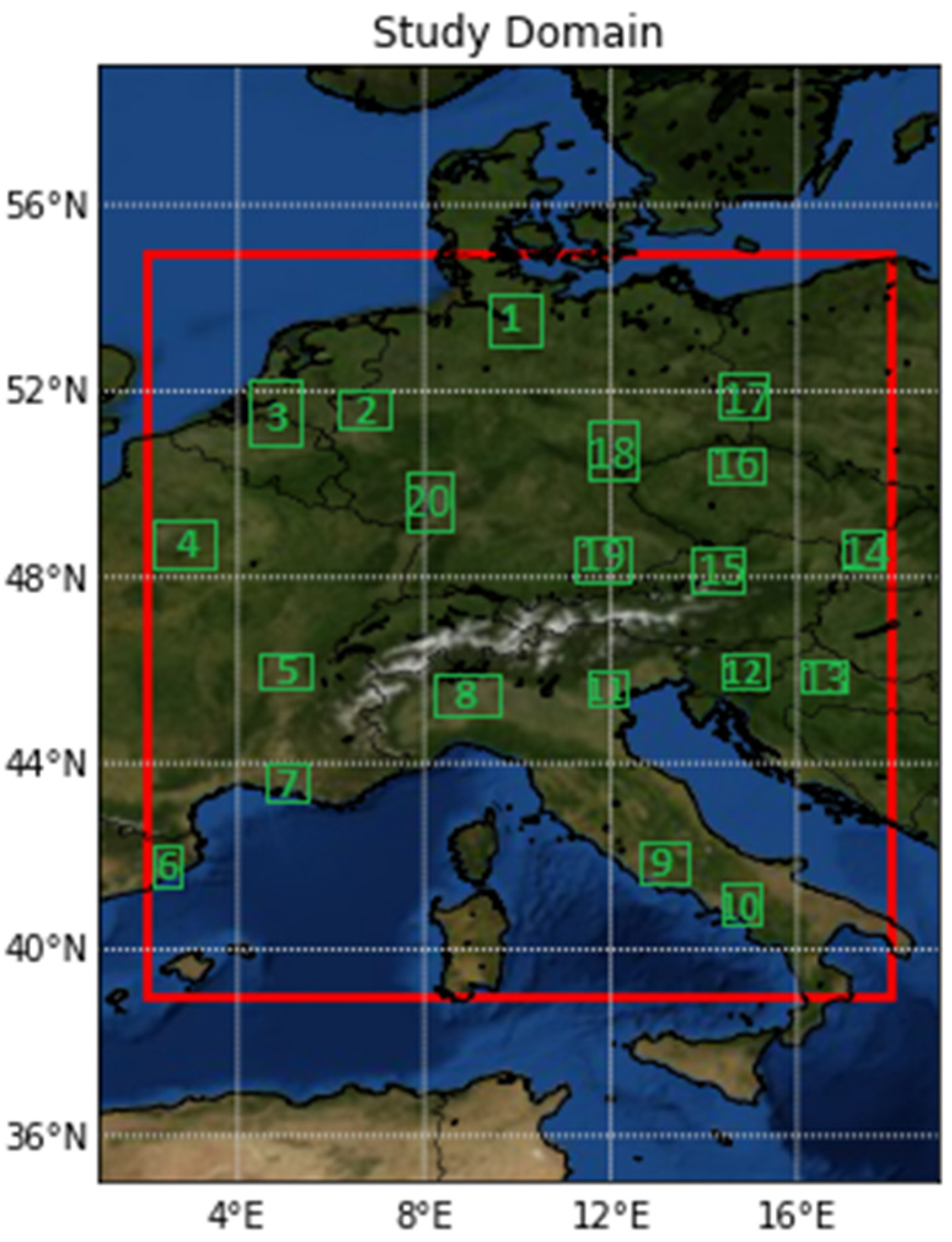
2.1.4. European Environmental Agency In Situ Measurements
2.2. Methodology
- So, inferred TROPOMI NO2 surface concentration;
- SG, NO2 surface concentration of the model;
- ΩG, NO2 tropospheric VCDs of the model;
- Ωο, NO2 tropospheric VCDs from the satellite observations.
3. Results
3.1. Investigation into Influencing Quantities
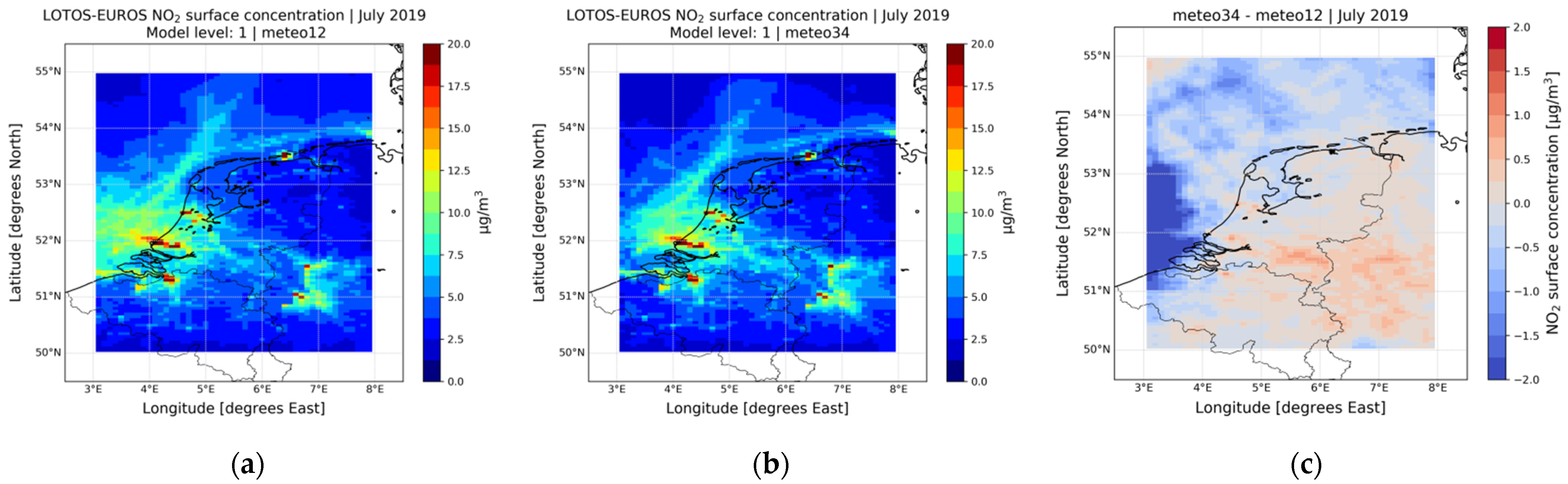
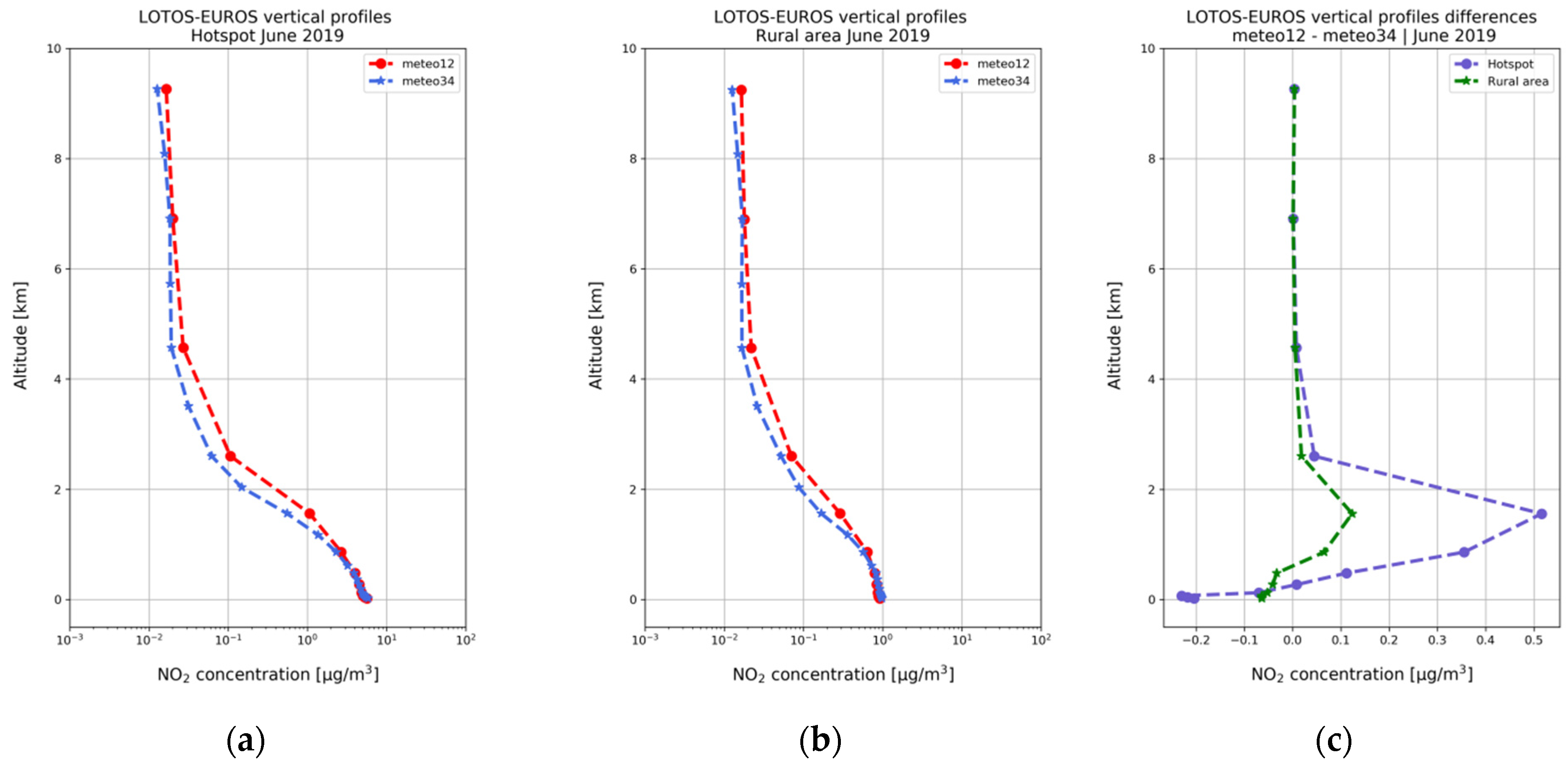
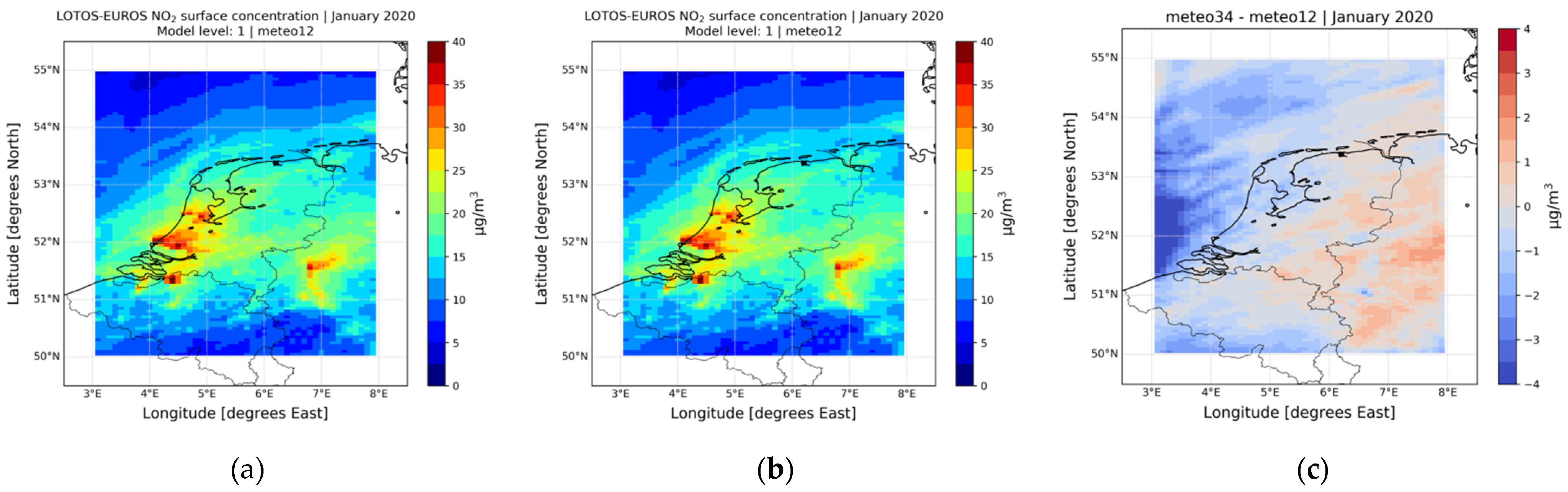
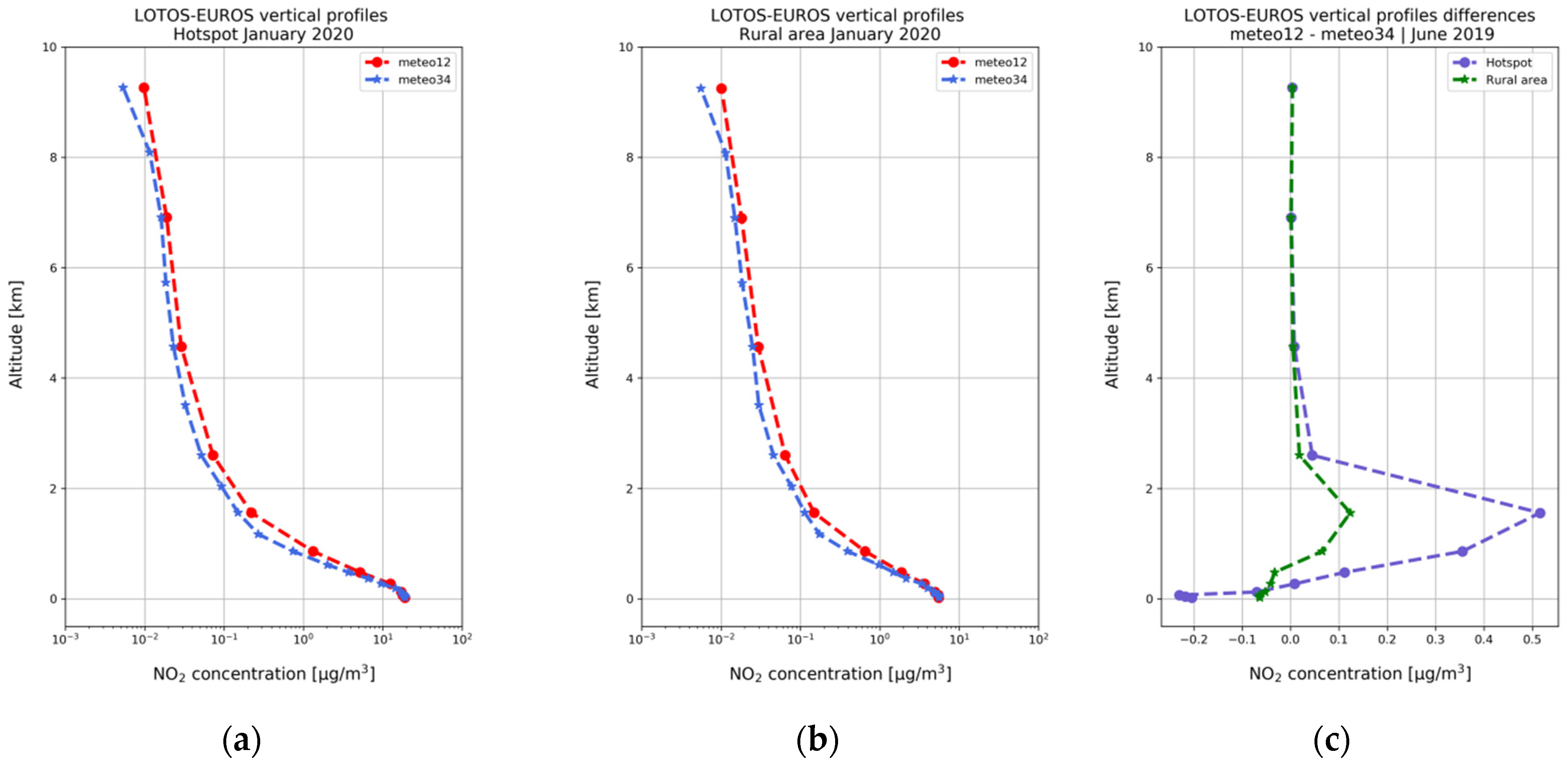
3.1.1. LOTOS-EUROS Vertical Leveling Scheme
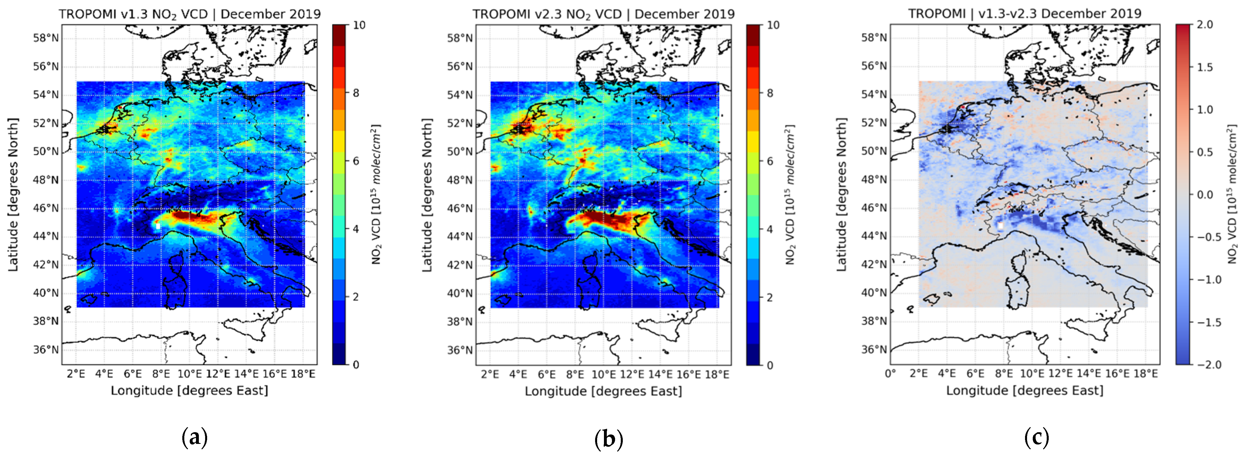
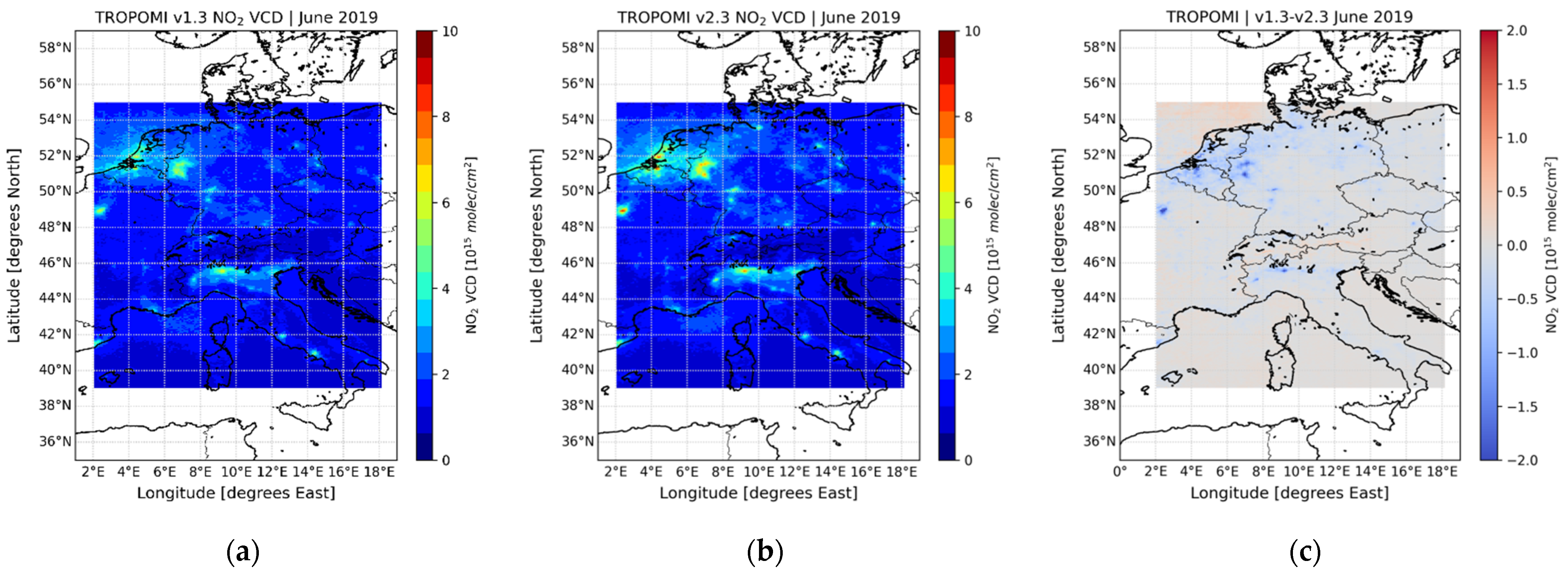
3.1.2. S5P/TROPOMI Versions Comparison
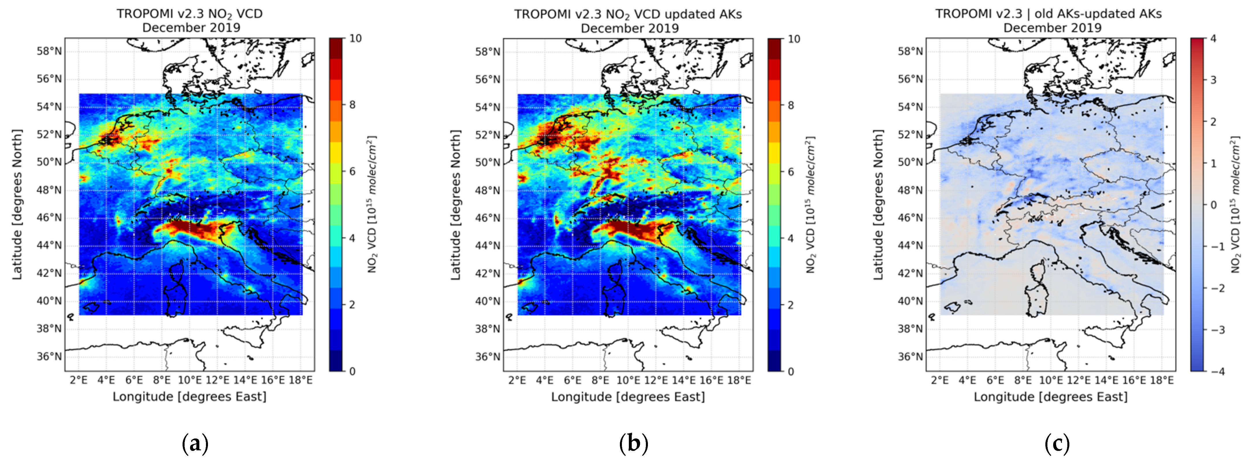
3.1.3. Application of the Updated Air Mass Factors
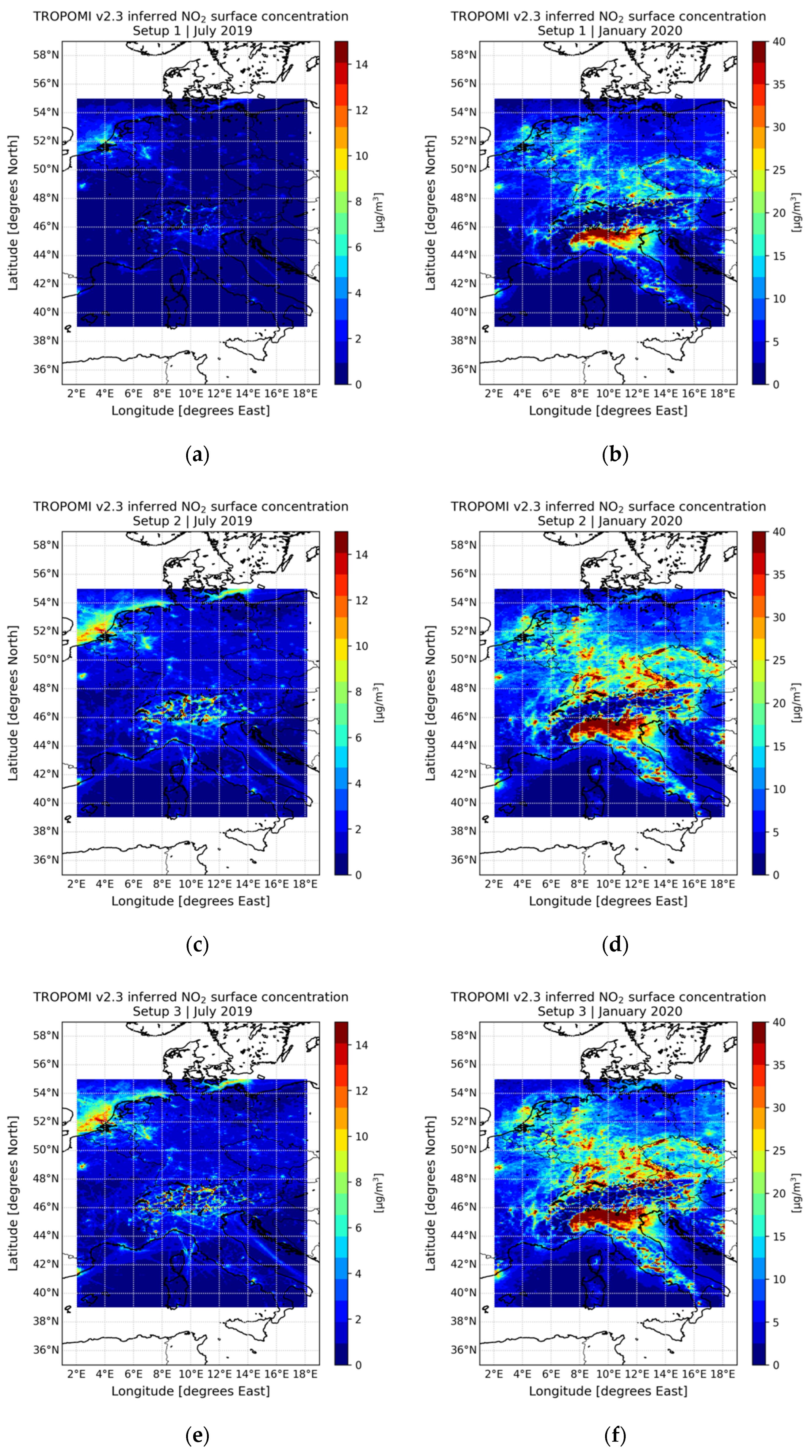
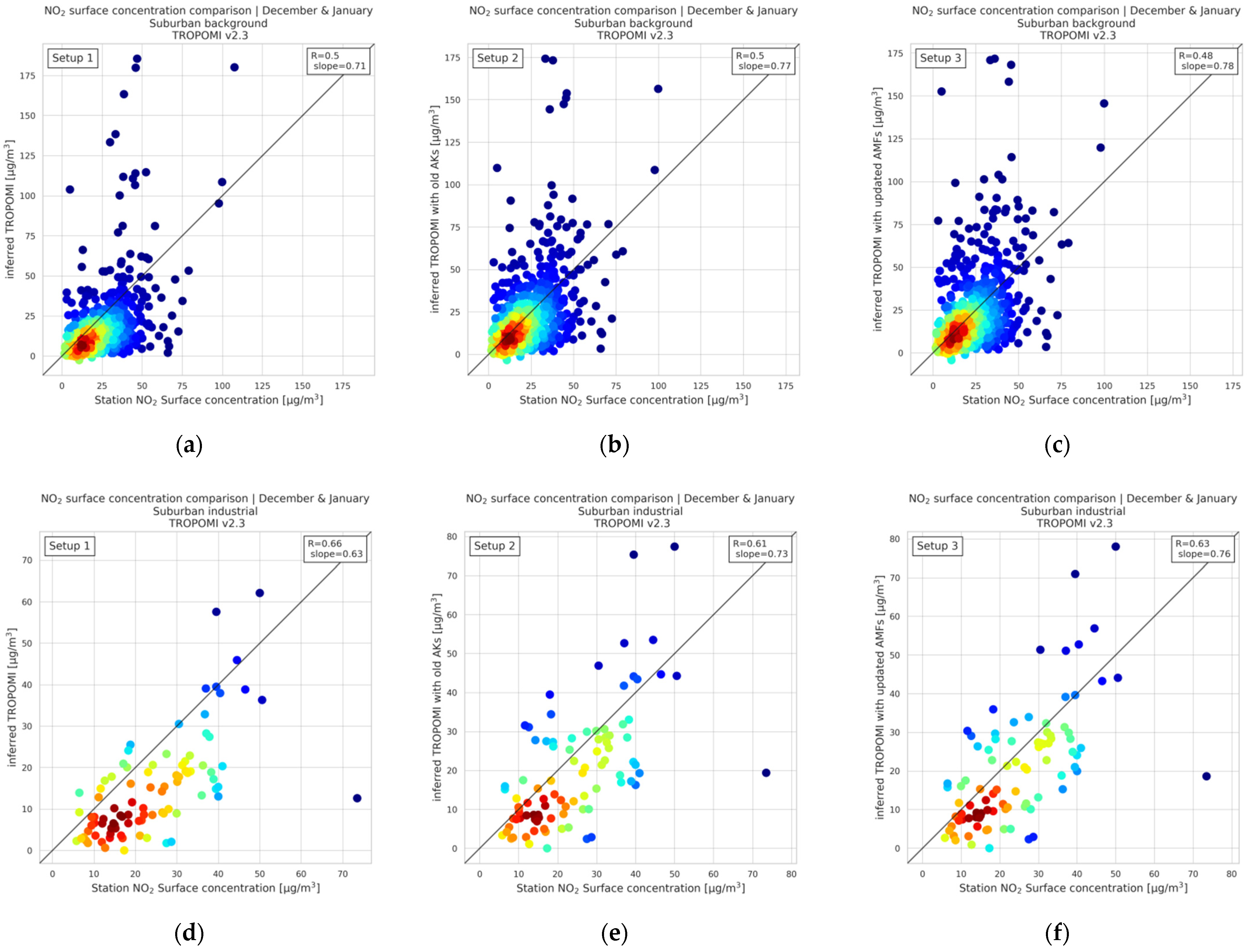
3.2. Optimal Setup
4. Conclusions
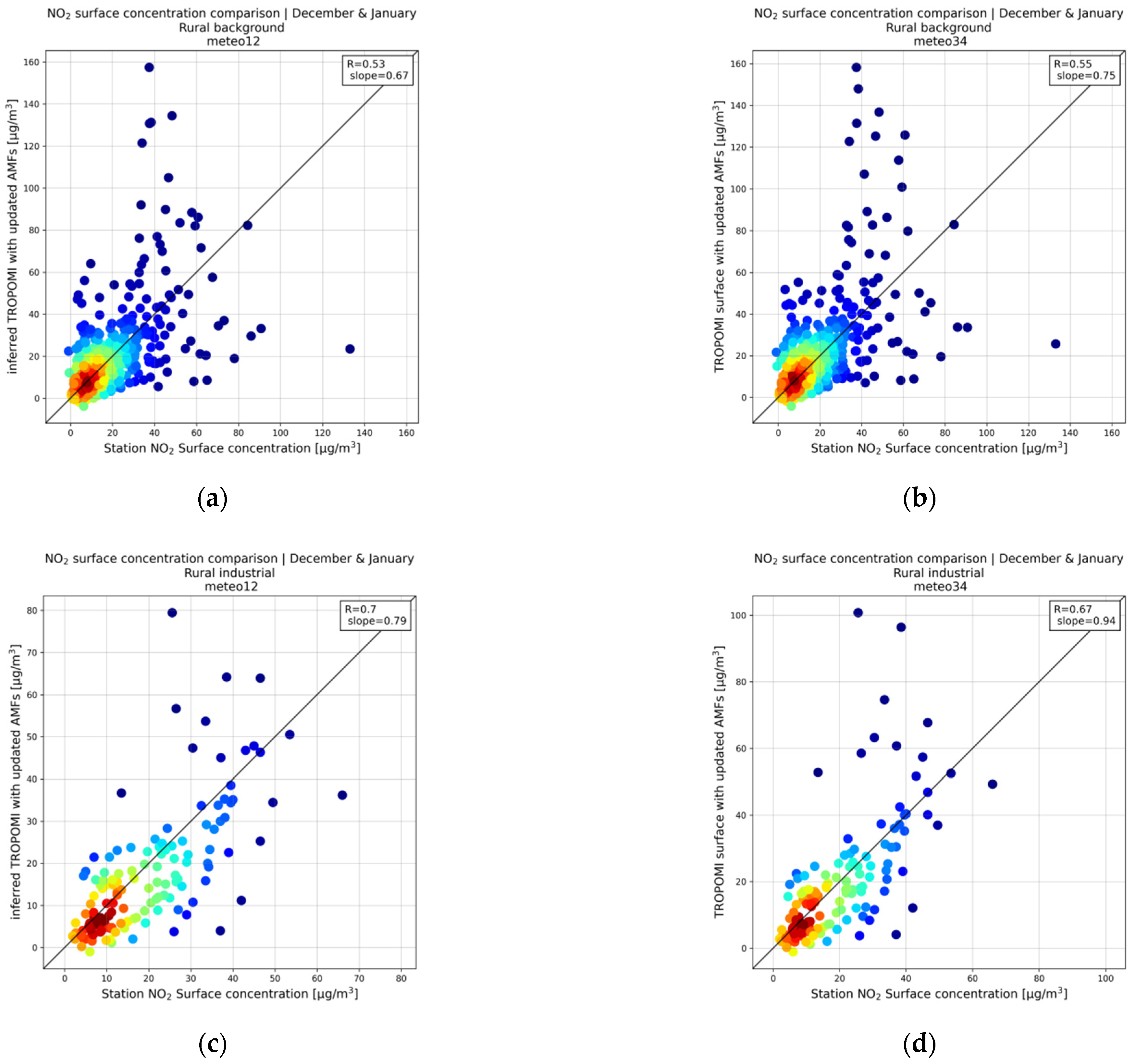
- The LOTOS-EUROS meteo34 vertical leveling scheme showed overall improved statistical indicators. Slopes are closer to 1, and the relative bias is lower. In particular, the relative bias in summer is lower for traffic stations by approximately 2%, for background stations by 7–9% and for the industrial stations by 5% compared to the relative bias of the meteo12 scheme. During winter, traffic and industrial stations relative bias is lower by 4–11%. Meteo34 background stations inferred NO2 TROPOMI v2.3 surface concentrations are higher by 5–7% compared to the meteo12. Overall, the meteo34 leveling scheme performs better, but it is computationally more expensive. Thus, the meteo12 leveling scheme was implemented in the further experiments.
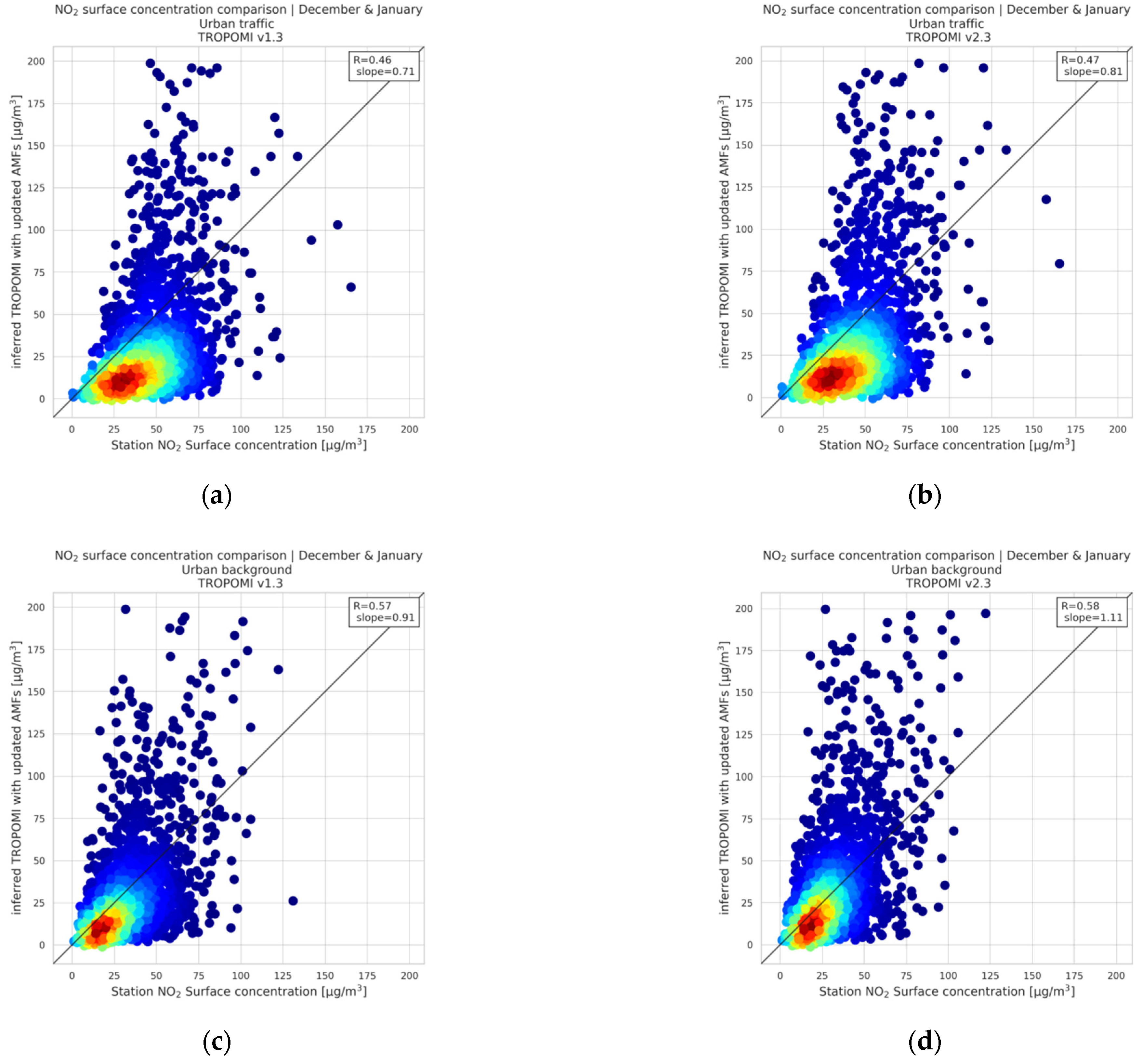
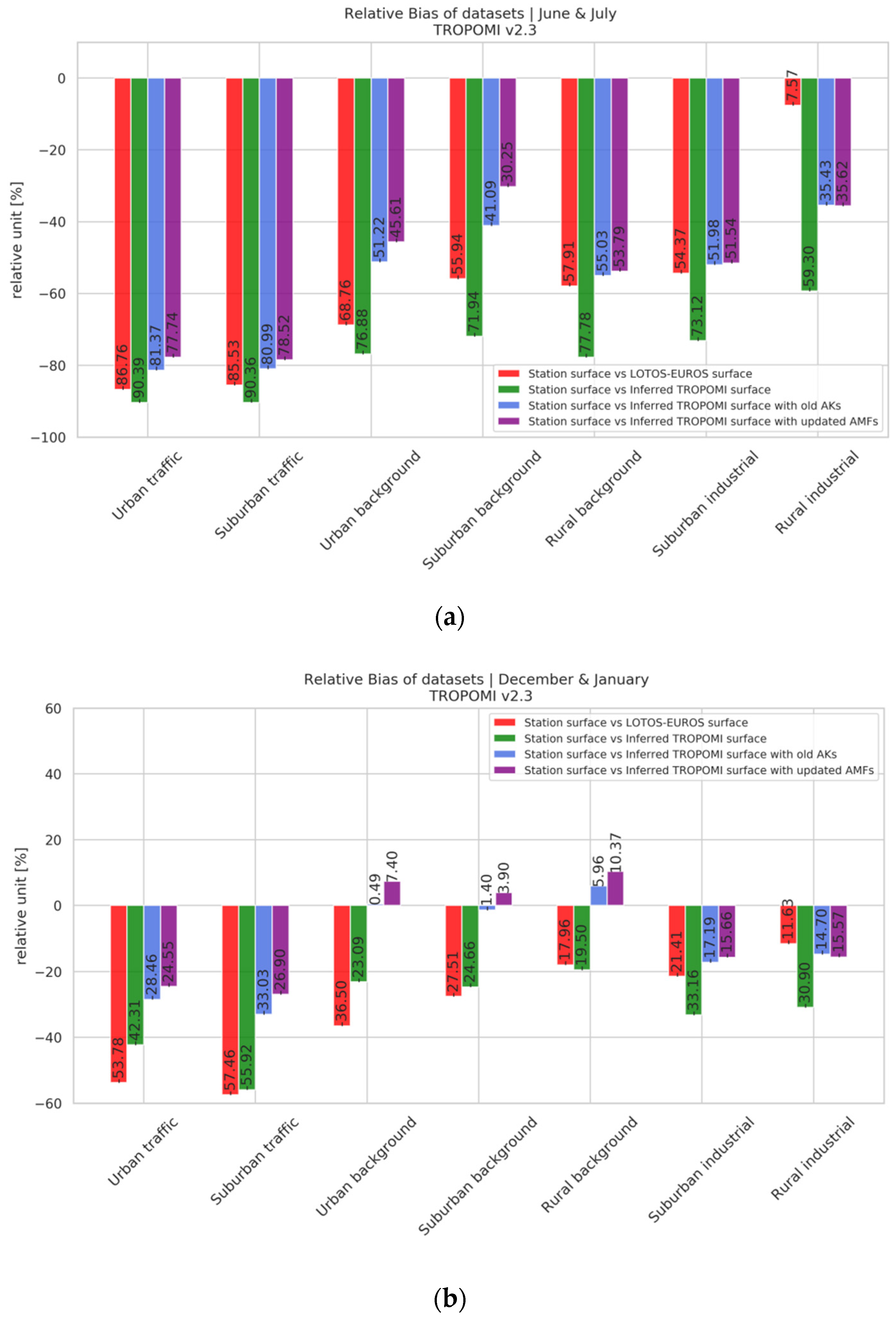
- TROPOMI v2.3-inferred NO2 surface concentrations showed overall better agreement with the ground-based measurements. The relative bias is lower by ~10% and ~18% for the traffic urban and suburban stations compared to the TROPOMI v1.3 -derived surface datasets. Urban and suburban background stations show a slightly lower bias of 5–6%, whereas the rural background stations bias is higher (~10%) than the TROPOMI v1.3 bias (~−0.25%). Finally, suburban- and rural- industrial-inferred TROPOMI v2.3 NO2 surface concentrations show an improved relative bias with the ground-based data (from ~−35% to ~15%).
- The derived TROPOMI v2.3 NO2 surface concentrations, updated with the air mass factors and averaging kernels from the local model (third setup), lie closer to the ground-based truth for both periods. In summer, biases are high for the traffic stations (~−70%) and moderate for background and industrial stations, ranging from −50% to −30%, improving significantly compared to the first setup. In winter, traffic and industrial stations bias improves from −50% to −25% and from −30% to −15%. Background-station-inferred NO2 surface concentrations slightly overestimate the ground-based measurements in winter. In this case, the second setup shows a lower bias for the urban (+0.49%), suburban (+1.40%) and rural (+5.96%) background stations compared to the third setup (+7.40%, +3.90% and +10.37%, respectively). This enhancement can be attributed to the sharper gradients included in the updated air mass factors. Comparisons between the first and the third setups show an average improvement of 24% and 18% in the bias of summer and winter, respectively.
- The implemented methodology performs better for the background and industrial stations for both periods. This may be attributed to the fact that TROPOMI and LOTOS-EUROS resolution is too low to properly resolve the high concentrations at traffic stations, resulting in higher net biases.
- Results are better in winter for all station types. Model simulations are obtained only at 11:00 UTC, which is the closest time to the TROPOMI overpass. The model underestimates the in situ NO2 surface concentrations during daytime and the underestimation is higher in summer. This might be attributed to the higher photolysis rate of NO2 in summer (higher solar radiation, low cloud cover), which is maximized in the early afternoon. Summer NO2 levels are significantly lower and closer to the emission sources compared to the winter, when the NOX lifetime is higher and local transport of emissions is more pronounced. Low resolution (0.10° × 0.05°) model simulations and satellite observations cannot detect emissions at station level, especially in summer, due to representation issues related to the location of the stations. Differences between both periods might also be partly attributed to the anthropogenic NOX emissions used in the model, as they refer to year 2017.
Author Contributions
Funding
Data Availability Statement
Acknowledgments
Conflicts of Interest
Appendix A


| New Leveling Scheme | Meteo Leveling Scheme | |||||
|---|---|---|---|---|---|---|
| Station Type | R | Slope | Relative Bias (%) | R | Slope | Relative Bias (%) |
| Urban traffic | 0.32 | 0.13 | −77.96% | 0.32 | 0.14 | −75.14% |
| Suburban traffic | 0.10 | 0.03 | −78.52% | 0.11 | 0.04 | −76.18% |
| Urban background | 0.46 | 0.38 | −45.68% | 0.45 | 0.42 | −38.90% |
| Suburban background | 0.52 | 0.49 | −30.58% | 0.50 | 0.54 | −21.04% |
| Rural background | 0.46 | 0.23 | −54.31% | 0.44 | 0.24 | −47.58% |
| Suburban industrial | 0.58 | 0.29 | −51.54% | 0.58 | 0.32 | −46.01% |
| Rural industrial | 0.63 | 0.34 | −37.47% | 0.61 | 0.36 | −32.30% |
| TROPOMI v1.3 | TROPOMI v2.3 | |||||
|---|---|---|---|---|---|---|
| Station Type | Slope | Absolute Bias * | Relative Bias (%) | Slope | Absolute Bias * | Relative Bias (%) |
| Urban traffic | 0.11 | 29.45 | −81.80% | 0.81 | 28.00 | −77.74% |
| Suburban traffic | 0.02 | 25.88 | −81.60% | 0.65 | 24.75 | −78.52% |
| Urban background | 0.31 | 7.98 | −56.50% | 1.11 | 6.35 | −45.61% |
| Suburban background | 0.39 | 4.82 | −43.77% | 0.78 | 3.27 | −30.25% |
| Rural background | 0.19 | 3.47 | −59.21% | 0.67 | 3.17 | −53.79% |
| Suburban industrial | 0.19 | 7.76 | −64.19% | 0.76 | 6.11 | −51.54% |
| Rural industrial | 0.23 | 4.40 | −49.90% | 0.79 | 3.02 | −36.62% |
References
- Seinfeld, J.H.; Pandis, S.N. Atmospheric Chemistry and Physics: From Air Pollution to Climate Change, 3rd ed.; Wiley: New York, NY, USA, 1998; pp. 724–743. [Google Scholar]
- Sheel, V.; Shyam, L.; Richter, A.; Burrows, J.P. Comparison of satellite observed tropospheric NO2 over India with model simulations. Atm. Environ. 2010, 44, 3314–3321. [Google Scholar] [CrossRef]
- Cohen, A.J.; Brauer, M.; Burnett, R.; Anderson, H.R.; Frostad, J.; Estep, K.; Balakrishnan, K.; Brunekreef, B.; Dandona, L.; Dandona, R.; et al. Estimates and 25-year trends of the global burden of disease attributable to ambient air pollution: An analysis of data from the Global Burden of Diseases Study 2015. Lancet 2017, 389, 1907–1918. [Google Scholar] [CrossRef]
- Brook, J.R.; Burnett, R.T.; Dann, T.F.; Cakmak, S.; Goldberg, M.S.; Fan, X.; Wheeler, A.J. Further interpretation of the acute effect of nitrogen dioxide observed in Canadian time-series studies. J. Expo. Sci. Environ. Epidemiol. 2007, 17, S36–S44. [Google Scholar] [CrossRef]
- Crouse, D.L.; Peters, P.A.; Hystad, P.; Brook, J.R.; van Donkelaar, A.; Martin, R.V.; Villeneuve, P.J.; Jerrett, M.; Goldberg, M.S.; Arden Pope, C.; et al. Ambient PM2.5, O3, and NO2 exposures and associations with mortality over 16 years of follow-up in the canadian census health and environment cohort (CanCHEC). Environ. Health Perspect. 2015, 123, 1180–1186. [Google Scholar] [CrossRef] [PubMed]
- Stavrakou, T.; Müller, J.F.; Boersma, K.F.; de Smedt, I.; van der A, R.J. Assessing the distribution and growth rates of NOx emission sources by inverting a 10-year record of NO2 satellite columns. Geophys. Res. Lett. 2008, 35, 1–5. [Google Scholar] [CrossRef]
- Ialongo, I.; Virta, H.; Eskes, H.; Hovila, J.; Douros, J. Comparison of TROPOMI/Sentinel-5 Precursor NO2 observations with ground-based measurements in Helsinki. Atmos. Meas. Tech. 2020, 13, 205–218. [Google Scholar] [CrossRef]
- Goldberg, D.L.; Anenberg, S.C.; Kerr, G.H.; Mohegh, A.; Lu, Z.; Streets, D.G. TROPOMI NO2 in the United States: A Detailed Look at the Annual Averages, Weekly Cycles, Effects of Temperature, and Correlation with Surface NO2 Concentrations. Earth’s Future 2021, 9, 1–16. [Google Scholar] [CrossRef]
- Lamsal, L.N.; Martin, R.V.; van Donkelaar, A.; Steinbacher, M.; Celarier, E.A.; Bucsela, E.; Dunlea, E.J.; Pinto, J.P. Ground-level nitrogen dioxide concentrations inferred from the satellite-borne Ozone Monitoring Instrument. J. Geo. Res. Atmos. 2008, 113, D16. [Google Scholar] [CrossRef]
- Lamsal, L.N.; Martin, R.V.; van Donkelaar, A.; Celarier, E.A.; Bucsela, E.J.; Boersma, K.F.; Dirksen, R.; Luo, C.; Wang, Y. Indirect validation of tropospheric nitrogen dioxide retrieved from the OMI satellite instrument: Insight into the seasonal variation of nitrogen oxides at northern midlatitudes. J. Geo. Res. Atmos. 2010, 115, D5. [Google Scholar] [CrossRef]
- Lamsal, L.N.; Duncan, B.N.; Yoshida, Y.; Krotkov, N.A.; Pickering, K.E.; Streets, D.G.; Lu, Z.U.S. NO2 trends (2005–2013): EPA Air Quality System (AQS) data versus improved observations from the Ozone Monitoring Instrument (OMI). Atmos. Environ. 2015, 110, 130–143. [Google Scholar] [CrossRef]
- Geddes, J.A.; Martin, R.V.; Boys, B.L.; van Donkelaar, A. Long-term trends worldwide in ambient NO2 concentrations inferred from satellite observations. Environ. Health Perspect. 2016, 124, 281–289. [Google Scholar] [CrossRef] [PubMed]
- Anand, J.S.; Monks, P.S. Estimating daily surface NO2 concentrations from satellite data—A case study over Hong Kong using land use regression models. Atmos. Chem. Phys. 2017, 17, 8211–8230. [Google Scholar] [CrossRef]
- Gu, J.; Chen, L.; Yu, C.; Li, S.; Tao, J.; Fan, M.; Xiong, X.; Wang, Z.; Shang, H.; Su, L. Ground-Level NO2 Concentrations over China Inferred from the Satellite OMI and CMAQ Model Simulations. Remote Sens. 2017, 9, 519. [Google Scholar] [CrossRef]
- Cooper, M.J.; Martin, R.V.; McLinden, C.A.; Brook, J.R. Inferring ground-level nitrogen dioxide concentrations at fine spatial resolution applied to the TROPOMI satellite instrument. Environ. Res. Lett. 2020, 15, 104013. [Google Scholar] [CrossRef]
- Cooper, M.J.; Martin, R.V.; Hammer, M.S.; Levelt, P.F.; Veefkind, P.; Lamsal, L.N.; Krotkov, N.A.; Brook, J.R.; McLinden, C.A. Global fine-scale changes in ambient NO2 during COVID-19 lockdowns. Nature 2022, 601, 380–387. [Google Scholar] [CrossRef]
- Kang, Y.; Choi, H.; Im, J.; Park, S.; Shin, M.; Song, C.K.; Kim, S. Estimation of surface-level NO2 and O3 concentrations using TROPOMI data and machine learning over East Asia. Environ. Poll. 2021, 288, 117711. [Google Scholar] [CrossRef]
- Ghahremanloo, M.; Lops, Y.; Choi, Y.; Yeganeh, B. Deep Learning Estimation of Daily Ground-Level NO2 Concentrations from Remote Sensing Data. J. Geo. Res. Atmos. 2021, 126, 1–18. [Google Scholar] [CrossRef]
- Chan, K.L.; Khorsandi, E.; Liu, S.; Baier, F.; Valks, P. Estimation of surface NO2 concentrations over germany from tropomi satellite observations using a machine learning method. Remote Sens. 2021, 13, 969. [Google Scholar] [CrossRef]
- Veefkind, J.P.; Aben, I.; McMullan, K.; Förster, H.; de Vries, J.; Otter, G.; Claas, J.; Eskes, H.J.; de Haan, J.F.; Kleipool, Q.; et al. TROPOMI on the ESA Sentinel-5 Precursor: A GMES mission for global observations of the atmospheric composition for climate, air quality and ozone layer applications. Remote Sens. Environ. 2012, 120, 70–83. [Google Scholar] [CrossRef]
- Van Geffen, J.; Boersma, K.F.; Eskes, H.; Sneep, M.; ter Linden, M.; Zara, M.; Veefkind, J.P. S5P Tropomi NO2 slant column retrieval: Method, stability, uncertainties and comparisons with OMI. Atmos. Meas. Tech. 2020, 13, 1315–1335. [Google Scholar] [CrossRef]
- Van Geffen, J.; Eskes, H.J.; Boermsa, K.F.; Veefkind, J.P. TROPOMI ATBD of the Total and Tropospheric NO2 Data Products. 2021. Available online: https://sentinel.esa.int/documents/247904/2476257/sentinel-5p-tropomi-atbd-no2-data-products (accessed on 25 September 2022).
- Van Geffen, J.; Eskes, H.; Compernolle, S.; Pinardi, G.; Verhoelst, T.; Lambert, J.-C.; Sneep, M.; ter Linden, M.; Ludewig, A.; Boersma, K.F.; et al. Sentinel-5P TROPOMI NO2 retrieval: Impact of version v2.3 improvements and comparisons with OMI and ground-based data. Atmos. Meas. Tech. 2022, 15, 2037–2060. [Google Scholar] [CrossRef]
- Beirle, S.; Borger, C.; Dörner, S.; Li, A.; Hu, Z.; Liu, F.; Wang, Y.; Wagner, T. Pinpointing nitrogen oxide emissions from space. Sci. Adv. 2019, 5, 1–7. [Google Scholar] [CrossRef] [PubMed]
- Stavrakou, T.; Müller, J.F.; Bauwens, M.; Boersma, K.F.; Van Geffen, J. Satellite evidence for changes in the NO2 weekly cycle over large cities. Sci. Rep. 2020, 10, A10066. [Google Scholar] [CrossRef] [PubMed]
- Koukouli, M.-E.; Skoulidou, I.; Karavias, A.; Parcharidis, I.; Balis, D.; Manders, A.; Segers, A.; Eskes, H.; van Geffen, J. Sudden changes in nitrogen dioxide emissions over Greece due to lockdown after the outbreak of COVID-19. Atmos. Chem. Phys. 2021, 21, 1759–1774. [Google Scholar] [CrossRef]
- Boersma, K.F.; Eskes, H.J.; Dirksen, R.J.; van der A, R.J.; Veefkind, J.P.; Stammes, P.; Huijnen, V.; Kleipool, Q.L.; Sneep, M.; Claas, J.; et al. An improved tropospheric NO2 column retrieval algorithm for the Ozone Monitoring Instrument. Atmos. Meas. Tech. 2011, 4, 1905–1928. [Google Scholar] [CrossRef]
- Boersma, K.F.; Eskes, H.J.; Richter, A.; De Smedt, I.; Lorente, A.; Beirle, S.; van Geffen, J.H.G.M.; Zara, M.; Peters, E.; Van Roozendael, M.; et al. Improving algorithms and uncertainty estimates for satellite NO2 retrievals: Results from the quality assurance for the essential climate variables (QA4ECV) project. Atmos. Meas. Tech. 2018, 11, 6651–6678. [Google Scholar] [CrossRef]
- Eskes, H.; van Geffen, J.; Boersma, K.F.; Eichmann, K.U.; Apituley, A.; Pedergnana, M.; Sneep, M.; Veefkind, J.P.; Loyola, D. Sentinel-5 Precursor/TROPOMI Level 2 Product User Manual. 2021. Available online: https://sentinel.esa.int/documents/247904/2474726/Sentinel-5P-Level-2-Product-User-Manual-Methane.pdf/1808f165-0486-4840-ac1d-06194238fa96 (accessed on 25 September 2022).
- Lambert, J.-C.; Keppens, A.; Compernolle, S.; Eichmann, K.-U.; de Graaf, M.; Hubert, D.; Langerock, B.; Ludewig, A.; Sha, M.K.; Verhoelst, T.; et al. Quarterly Validation Report of the Copernicus Sentinel-5 Precursor Operational Data Products #14: April 2018 March 2022. S5P MPC Routine Operations Consolidated Validation Report Series, Issue #14, Version 14.01.01. 6 April 2022. Available online: http://www.tropomi.eu/sites/default/files/files/publicS5P-MPC-IASB-ROCVR-06.0.1-20200330_FINAL.pdf (accessed on 25 September 2022).
- Manders, A.M.M.; Builtjes, P.J.H.; Curier, L.; Denier van der Gon, H.A.C.; Hendriks, C.; Jonkers, S.; Kranenburg, R.; Kuenen, J.J.P.; Segers, A.J.; Timmermans, R.M.A.; et al. Curriculum vitae of the LOTOS–EUROS (v2.0) chemistry transport model. Geosci. Model Dev. 2017, 10, 4145–4173. [Google Scholar] [CrossRef]
- Schaap, M.; Timmermans, R.M.A.; Roemer, M.; Boersen, G.A.C.; Builtjes, P.J.H.; Sauter, F.J.; Velders, G.J.M.; Beck, J.P. The LOTOS-EUROS model: Description, validation and latest developments. Inter. J. Environ. Poll. 2008, 32, 270–290. [Google Scholar] [CrossRef]
- Skoulidou, I.; Koukouli, M.-E.; Manders, A.; Segers, A.; Karagkiozidis, D.; Gratsea, M.; Balis, D.; Bais, A.; Gerasopoulos, E.; Stavrakou, T.; et al. Evaluation of the LOTOS-EUROS NO2 simulations using ground-based measurements and S5P/TROPOMI observations over Greece. Atmos. Chem. Phys. 2021, 21, 5269–5288. [Google Scholar] [CrossRef]
- Skoulidou, I.; Koukouli, M.-E.; Segers, A.; Manders, A.; Balis, D.; Stavrakou, T.; van Geffen, J.; Eskes, H. Changes in Power Plant NOx Emissions over Northwest Greece Using a Data Assimilation Technique. Atmosphere 2021, 12, 900. [Google Scholar] [CrossRef]
- Pseftogkas, A.; Koukouli, M.-E.; Skoulidou, I.; Balis, D.; Meleti, C.; Stavrakou, T.; Falco, L.; van Geffen, J.; Eskes, H.; Segers, A.; et al. A New Separation Methodology for the Maritime Sector Emissions over the Mediterranean and Black Sea Regions. Atmosphere 2021, 12, 1478. [Google Scholar] [CrossRef]
- Hersbach, H.; Bell, B.; Berrisford, P.; Biavati, G.; Dee, D.; Horányi, A.; Nicolas, J.; Peubey, C.; Radu, R.; Rozum, I.; et al. The ERA5 Global Atmospheric Reanalysis at ECMWF as a comprehensive dataset for climate data homogenization, climate variability, trends and extremes. Geo. Res. Abstr. 2020, 21, 1. [Google Scholar] [CrossRef]
- Granier, C.; Darras, S.; van der Gon, H.D.; Doubalova, J.; Elguindi, N.; Galle, B.; Gauss, M.; Guevara, M.; Jalkanen, J.-P.; Kuenen, J.; et al. The Copernicus Atmosphere Monitoring Service Global and Regional Emissions (April 2019 Version), Copernicus Atmosphere Monitoring Service (CAMS) Report. 2019. Available online: https://atmosphere.copernicus.eu/sites/default/files/2019-06/cams_emissions_general_document_apr2019_v7.pdf (accessed on 25 September 2022).
- Williams, J.E.; Boersma, K.F.; Le Sager, P.; and Verstraeten, W.W. The high-resolution version of TM5-MP for optimized satellite retrievals: Description and validation. Geosci. Model Dev. 2017, 10, 721–750. [Google Scholar] [CrossRef]
- Segers, A.; Manders, A.; Kranenburg, R. LOTOS-EUROS User Guide v2.3.000. 2019. Available online: https://lotos-euros.tno.nl/media/10360/reference_guide_v2-0_r10898.pdf (accessed on 25 September 2022).
- Segers, A.; Jonkers, S.; Schaap, M.; Timmermans, R.; Hendriks, C.; Sauter, F.; Kruit, R.W.; van der Swaluw, E.; Eskes, H.; Banzhaf, S. LOTOS-EUROS v2.3.000 Reference Guide. 2019. Available online: https://lotos-euros.tno.nl/media/10360/reference_guide_v2-0_r10898.pdf (accessed on 25 September 2022).


| Datasets | Setup 1/Baseline | Setup 2 | Setup 3 |
|---|---|---|---|
| LOTOS-EUROS | A priori NO2 surface concentrations and a priori NO2 VCDs | NO2 surface concentrations and NO2 VCDs with TM5-MP AKs | A priori NO2 surface concentrations and NO2 VCDs with updated AMFs and AKs |
| TROPOMI | Original NO2 VCD | Original NO2 VCD | NO2 VCD with updated AMFs and AKs |
| Surface products | TROPOMI inferred NO2 surface concentration | TROPOMI inferred NO2 surface concentrations with TM5-MP AKs | TROPOMI inferred NO2 surface concentrations with model air mass factors correction |
| Meteo12 Leveling Scheme | Meteo34 Leveling Scheme | |||||
|---|---|---|---|---|---|---|
| Station Type | R | Slope | Relative Bias (%) | R | Slope | Relative Bias (%) |
| Urban traffic | 0.47 | 0.81 | −24.55% | 0.48 | 0.85 | −20.70% |
| Suburban traffic | 0.43 | 0.65 | −26.90% | 0.45 | 0.69 | −23.18% |
| Urban background | 0.58 | 1.11 | +7.40% | 0.58 | 1.13 | +12.00% |
| Suburban background | 0.48 | 0.78 | +3.90% | 0.49 | 0.86 | +10.90% |
| Rural background | 0.53 | 0.67 | +10.37% | 0.55 | 0.75 | +18.29% |
| Suburban industrial | 0.63 | 0.76 | −15.66% | 0.62 | 0.82 | −9.70% |
| Rural industrial | 0.7 | 0.79 | −15.57% | 0.67 | 0.94 | −4.32% |
| TROPOMI v1.3 | TROPOMI v2.3 | |||||
|---|---|---|---|---|---|---|
| Station Type | Slope | Absolute Bias * | Relative Bias (%) | Slope | Absolute Bias * | Relative Bias (%) |
| Urban traffic | 0.71 | 15.46 | −35.41% | 0.81 | 10.64 | −24.55% |
| Suburban traffic | 0.48 | 20.19 | −44.93% | 0.65 | 11.53 | −26.90% |
| Urban background | 0.91 | 3.86 | −12.78% | 1.11 | −2.21 | 7.40% |
| Suburban background | 0.73 | 2.27 | −9.94% | 0.78 | −0.89 | 3.90% |
| Rural background | 0.66 | 0.05 | −0.25% | 0.67 | −1.97 | 10.37% |
| Suburban industrial | 0.56 | 7.46 | −31.79% | 0.76 | 3.77 | −15.66% |
| Rural industrial | 0.59 | 7.55 | −38.03% | 0.79 | 3.05 | −15.57% |
| Summer | Winter | |||||
|---|---|---|---|---|---|---|
| Station Type | In Situ | Setup 1 | Setup 3 | In Situ | Setup 1 | Setup 3 |
| Urban traffic | 36.02 ± 6.00 | 3.46 ± 1.86 | 8.02 ± 2.83 | 43.34 ± 6.58 | 25.00 ± 5.00 | 32.70 ± 5.72 |
| Suburban traffic | 31.52 ± 5.61 | 3.04 ± 1.74 | 6.77 ± 2.60 | 42.87 ± 6.55 | 18.90 ± 4.35 | 31.34 ± 5.60 |
| Urban background | 13.92 ± 3.73 | 3.21 ± 1.79 | 7.57 ± 2.75 | 29.30 ± 5.48 | 23.06 ± 4.80 | 32.20 ± 5.67 |
| Suburban background | 10.81 ± 3.29 | 3.03 ± 1.74 | 7.54 ± 2.75 | 22.85 ± 4.78 | 17.21 ± 4.15 | 23.73 ± 4.87 |
| Rural background | 5.90 ± 2.43 | 1.31 ± 1.15 | 2.73 ± 1.65 | 18.96 ± 4.35 | 15.27 ± 3.91 | 20.93 ± 4.87 |
| Suburban industrial | 11.86 ± 3.44 | 3.19 ± 1.79 | 5.75 ± 2.40 | 24.06 ± 4.91 | 16.08 ± 4.01 | 20.29 ± 4.58 |
| Rural industrial | 8.49 ± 2.91 | 3.45 ± 1.86 | 5.47 ± 2.34 | 19.59 ± 4.43 | 13.53 ± 3.68 | 16.54 ± 4.07 |
Publisher’s Note: MDPI stays neutral with regard to jurisdictional claims in published maps and institutional affiliations. |
© 2022 by the authors. Licensee MDPI, Basel, Switzerland. This article is an open access article distributed under the terms and conditions of the Creative Commons Attribution (CC BY) license (https://creativecommons.org/licenses/by/4.0/).
Share and Cite
Pseftogkas, A.; Koukouli, M.-E.; Segers, A.; Manders, A.; Geffen, J.v.; Balis, D.; Meleti, C.; Stavrakou, T.; Eskes, H. Comparison of S5P/TROPOMI Inferred NO2 Surface Concentrations with In Situ Measurements over Central Europe. Remote Sens. 2022, 14, 4886. https://doi.org/10.3390/rs14194886
Pseftogkas A, Koukouli M-E, Segers A, Manders A, Geffen Jv, Balis D, Meleti C, Stavrakou T, Eskes H. Comparison of S5P/TROPOMI Inferred NO2 Surface Concentrations with In Situ Measurements over Central Europe. Remote Sensing. 2022; 14(19):4886. https://doi.org/10.3390/rs14194886
Chicago/Turabian StylePseftogkas, Andreas, Maria-Elissavet Koukouli, Arjo Segers, Astrid Manders, Jos van Geffen, Dimitris Balis, Charikleia Meleti, Trissevgeni Stavrakou, and Henk Eskes. 2022. "Comparison of S5P/TROPOMI Inferred NO2 Surface Concentrations with In Situ Measurements over Central Europe" Remote Sensing 14, no. 19: 4886. https://doi.org/10.3390/rs14194886
APA StylePseftogkas, A., Koukouli, M.-E., Segers, A., Manders, A., Geffen, J. v., Balis, D., Meleti, C., Stavrakou, T., & Eskes, H. (2022). Comparison of S5P/TROPOMI Inferred NO2 Surface Concentrations with In Situ Measurements over Central Europe. Remote Sensing, 14(19), 4886. https://doi.org/10.3390/rs14194886