Article

Flood Hazard Analysis Based on Rainfall Fusion: A Case Study in Dazhou City, China

1
Institute for Disaster Management and Reconstruction, Sichuan University, No. 122 Huanghe Middle Road Section 1, Chengdu 610207, China
2
State Key Laboratory of Hydraulics and Mountain River Engineering, College of Water Resource & Hydropower, Sichuan University, No. 24 South Section 1, Yihuan Road, Chengdu 610065, China
3
College of Water Resources and Hydropower, Sichuan Agricultural University, Ya’an 625014, China
4
Sichuan Jiangyuan Engineering Consulting Co., Ltd., Chengdu 610041, China
*
Author to whom correspondence should be addressed.
These authors contributed equally to this work.
Remote Sens. 2022, 14(19), 4843; https://doi.org/10.3390/rs14194843
Submission received: 18 July 2022 / Revised: 5 September 2022 / Accepted: 27 September 2022 / Published: 28 September 2022
(This article belongs to the Special Issue Remote Sensing in Urban Flooding Monitoring)

Abstract

:
In recent years, extreme weather events caused by global climate change have occurred frequently, intensifying the frequency of flood disasters. For flood hazard analysis, high-quality data and a reasonable weight assignment of the relevant factors are critical. This study conducts four rainfall fusion methods, to fuse the Tropical Rainfall Measuring Mission (TRMM) 3B42 and the observations in Dazhou City, China. Then, the random forest was applied to obtain the weights of various factors to facilitate a comprehensive flood hazard analysis under four rainfall durations. The results show that (1) the linear regression performs best out of the four fusion methods, with a correlation coefficient of 0.56; (2) the Digital Elevation Model (DEM) is the most impact factor with a weight of more than 0.2; and (3) the proposed flood analysis system performs well, as 70% of historical flood points are distributed in high and sub-high hazard areas and more than 93% of historical flood points are distributed in medium hazard areas. This study identified the flood hazard grade and distribution in Dazhou City, which could provide a valuable methodology to contribute to flood hazard analysis and disaster management with satellite rainfall. Furthermore, the results of this paper are profound for future work on the high-resolution flood risk assessment and management in Dazhou City.

1. Introduction

A flood disaster is a complex phenomenon closely related to the natural environment and the human social system [1]. The hazard and frequency of floods and their impacts are expected to increase, especially in the low latitudes of Africa and Asia [2,3,4,5], owing to climate change, population growth, and economic development. Although many structural and non-structural measures have been proposed to reduce flood damage, the effects of flood hazards remain impactful at the county level [6]. As one of the countries most threatened by flood disasters, China suffered 125 major disasters from 1950 to 2004, with 1.465 billion people affected and USD 11.675 billion in losses [7], which seriously restricts the sustainable development of China’s economy [8,9]. Liu et al. [10] counted the number of flood disasters in seven major river basins in China in the past 150 years and found that each basin had witnessed more than 20, especially the Yangtze River and Yellow River basins. Since the 21st century, the significant damage and loss caused by flood disasters has still been a severe problem to be solved. Thus, it is urgent to improve the accuracy of the research related to flood disasters and to develop scientific and practical measures for flood control and disaster reduction [11,12,13].
Flood disaster research based on historical statistical data often uses statistical methods, such as time series and regression analysis, to clarify the distribution law and develop flood disaster trends for effective countermeasures [14,15]. The early warning and assessment of flood disasters have always been a hotspot in flood research [16,17]. Researchers try to use remote sensing technology to quickly obtain flood disaster information, such as the degree [18], time [19], dynamic characteristics of floods [20], and flooded social attributes such as affected houses, population, crops, and infrastructure [21,22,23]. Then, combined with historical disaster data and GIS technology, the scope, nature, and degree of a flood disaster hazard are analyzed by using an artificial neural network [24,25], random forest [26,27], and analytic hierarchy process [28,29].
A flood hazard analysis, as the essential element of flood control assessment, is crucial for the prediction and early warning of regional flood disasters [30]. Moreover, identifying the flood factors, such as rainfall, topography, and the distribution of river networks, is the most critical step of a flood hazard analysis [31,32]. Yalcin et al. [33] selected seven natural factors, including the annual rainfall, watershed size, basin slope, gradient of the main drainage channel, drainage density, land use, and soil types for the assessment of a flood hazard. Stefanidis et al. [34] added three anthropogenic factors related to human intrusion and flood control technology, increasing the number of considered flood hazard factors to 10. Moreover, multi-criteria analysis methods were proposed by Ologunorisa [35], Mansor et al. [36], and Sanyal and Lu [37] to combine the factors related to a flood hazard. However, none of them considered the importance of each factor, which is necessary for an accurate flood hazard analysis.
Rainfall significantly impacts a flood hazard analysis, especially heavy rainfall for a short period, as it is the most critical and direct cause of a flood disaster [38,39]. The rainfall data currently used for a flood hazard analysis is mainly collected from gauge observation and satellite estimation [40,41,42,43]. However, due to the uneven distribution of the rainfall gauges and the low accuracy of satellite data, the accuracy of precipitation for a flood hazard analysis is insufficient [44,45,46,47]. Therefore, obtaining highly accurate and wide-ranging rainfall data is a meaningful way to improve the ability of a flood hazard analysis, which could be beneficial in reducing the impact of flood disasters.
Rainfall data fusion is an effective and feasible way to improve the accuracy of satellite rainfall data [48,49,50]. The commonly used fusion methods can be divided into two categories. One is simple correction methods, such as Mean Bias Correction (MBC) [51], Double-Kernel Smoothing (DS) [52], and Linear Regression (LR) [53]; another is local correction methods, such as Optimum Interpolation (OI) [54], Kalman Filter (KF) [55], and Geographically Weighted Regression (GWR) [56]. Liu et al. [57] applied the LR method to fuse the TRMM 3B42 data and gauge rainfall data in China, and the accuracies of this fusion rainfall data were improved at the monthly and annual scales. Li et al. [58] fused the rainfall data from TRMM 3B42 and gauges in Australia by using the DS method. The cross-validation results showed that the DS method could improve the accuracy of the fusion rainfall. Duan et al. [59] employed LR, GWR, and KF to fuse the TRMM 3B42 and the gauges in Sichuan Province, China. The results showed that LR had the best merging effect at both the daily and monthly scales, while the KF presented the highest accuracy. It can be found that the optimal fusion method is not unique for TRMM 3B42 rainfall data in various study areas, due to the different climatic characteristics. Therefore, exploring the appropriate method to fuse rainfall data in a specific area with a few gauges is necessary. Moreover, the selection of hazard factors and their evaluation is critical for aflood hazard analysis.
This paper aims to conduct a flood hazard analysis based on the fused rainfall data and nine hazard factors, to solve the low accuracy rainfall and incomprehensive flood hazard evaluation in Dazhou City, Sichuan Province, China. This study employs four fusion methods, OI, GWR, KF, and LR, for fusing the TRMM 3B42 satellite rainfall and the gauge rainfall. After clarifying the applicable fusion method, it can be applied to obtain the fusion rainfall, solving the defects of uneven distribution, limited range, and low precision. Moreover, we propose a system for determining the weights of flood hazard factors and performing a flood analysis in this paper. Considering that few researchers have studied the impact of the instantaneity of rainfall on flood hazard, we set up four rainfall durations (3 h, 6 h, 9 h, and 12 h) according to the time scale of the TRMM 3B42 data and then carried out our flood hazard analysis. This study provides a new method for the hazard assessment of frequent flood disasters and is of great significance for the acquisition of guidelines for disaster management.

2. Study Area and Materials

2.1. Study Area

Dazhou City, located in the eastern part of Sichuan Province, between the longitude of 106°39′–108°32′ and the latitude of 30°19′–32°20′, is one of the major cities in southwest China, as shown in Figure 1. It is called the “East Gate” of Sichuan Province, with a population of more than five million, due to its advantaged location at the junction of Sichuan Province, Chongqing City, Hubei Province, and Shanxi Province. Moreover, it lies in the Chengdu–Chongqing Economic Belt, in the upper reaches of the Yangtze River. The topography of Dazhou City decreases from the Daba Mountain in the northeast to the hilly areas in the southwest, with an elevation range from 2458.30 to 222 m. The terrain in Dazhou City is classified into three types, i.e., mountainous areas (which account for 70.70% of Dazhou City’s area), hilly areas (28.10%), and flat areas (1.20%).
As the climatic boundary between north and south China, Dazhou City has a subtropical humid monsoon climate with frequent droughts and floods in summer and continuous rains in autumn. It has a forest coverage of 44.34% and annual average precipitation of about 1200 mm. It is hot and rainy simultaneously, and the annual average temperature is between 14.7 and 17.6 °C. Due to the complex terrain, the regional climate varies greatly. The low mountains, hills, and valleys below 800 m have a mild climate and four distinct seasons; the low and middle mountain areas with an elevation of 800 to 1000 m are cool and damp; and the middle mountains above 1000 m have a long cold period with insufficient sunlight and heat resources.

2.2. Materials

2.2.1. Rainfall Data

The satellite rainfall product used in this study is TRMM 3B42, with a spatial resolution of 0.25° and temporal resolution of 3 h, provided by the National Aeronautics and Space Administration (NASA) Goddard Earth Sciences (GES) Data and Information Services Center (DISC) (https://disc.gsfc.nasa.gov/datasets (accessed on 6 August 2021)) [60]. This data range covers the period from 1998 to 2019 [61,62]. The process of the original TRMM 3B42 data with HDF format is accomplished using the MATLAB program.
Rainfall gauge data of 3 h precipitation observations (from 1986 to 2012) of the seven rainfall stations over Dazhou City are provided by the China Meteorological Administration (CMA). According to the rain gauge distribution (Figure 1), the XuanHan station located in the center was chosen as the test point. The observed rainfall from the remaining six stations is interpolated using the inverse distance weighting method (IDW) [63,64], to generate grid gauge data, which has the exact spatial resolution as the grid satellite data. Moreover, the latitude and longitude coordinates of the rainfall gauges in the study area are counted to facilitate single-point data fusion.

2.2.2. Historical Flood Points

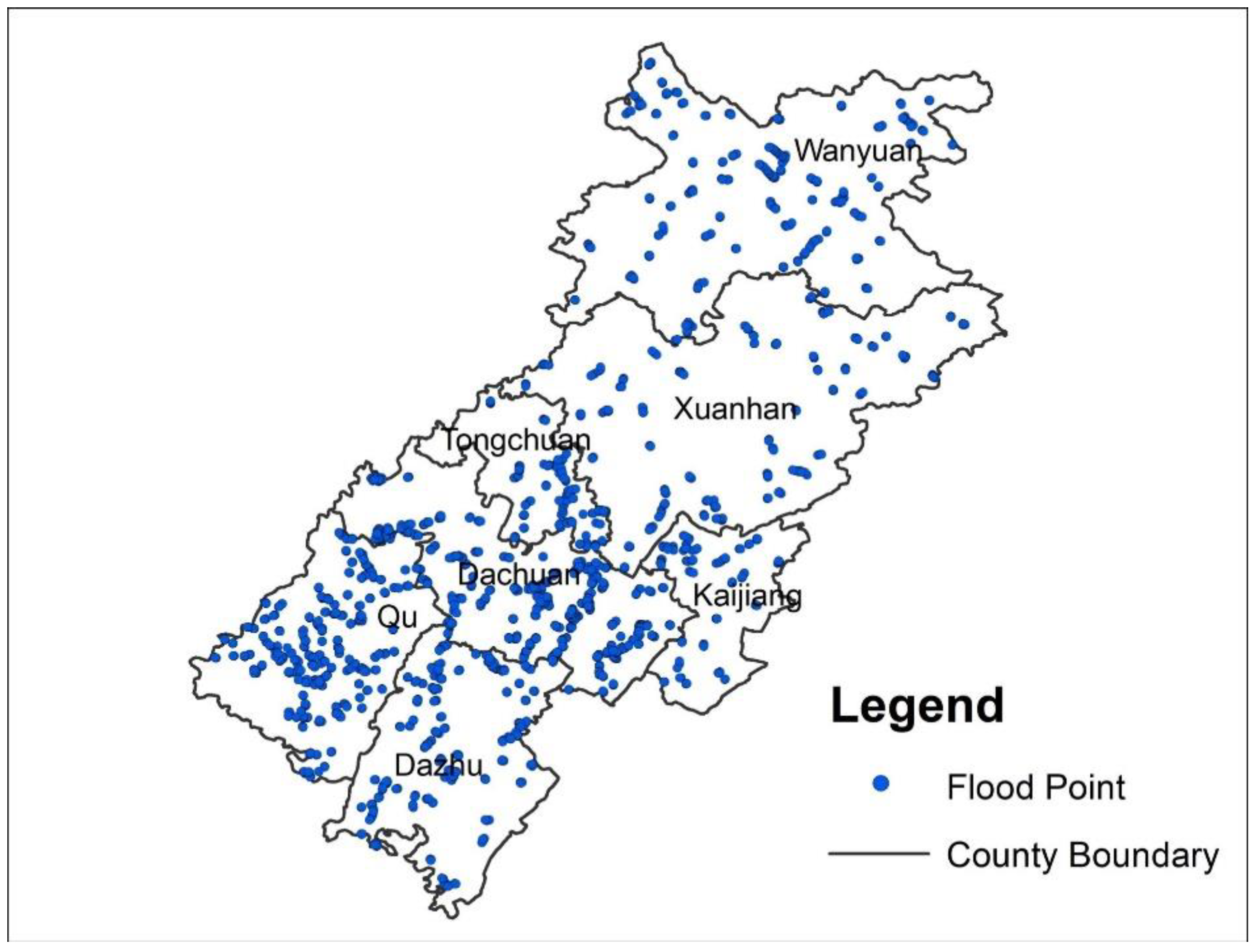
To evaluate the accuracy of the flood hazard analysis results, we collected historical flood data from 1952 to 2019 from the Dazhou Water Authority. According to the flood information, a total of 2254 historical flood points are shown in Figure 2, by counting the flood disaster locations and vectorizing them on ArcGIS.

3. Methodology

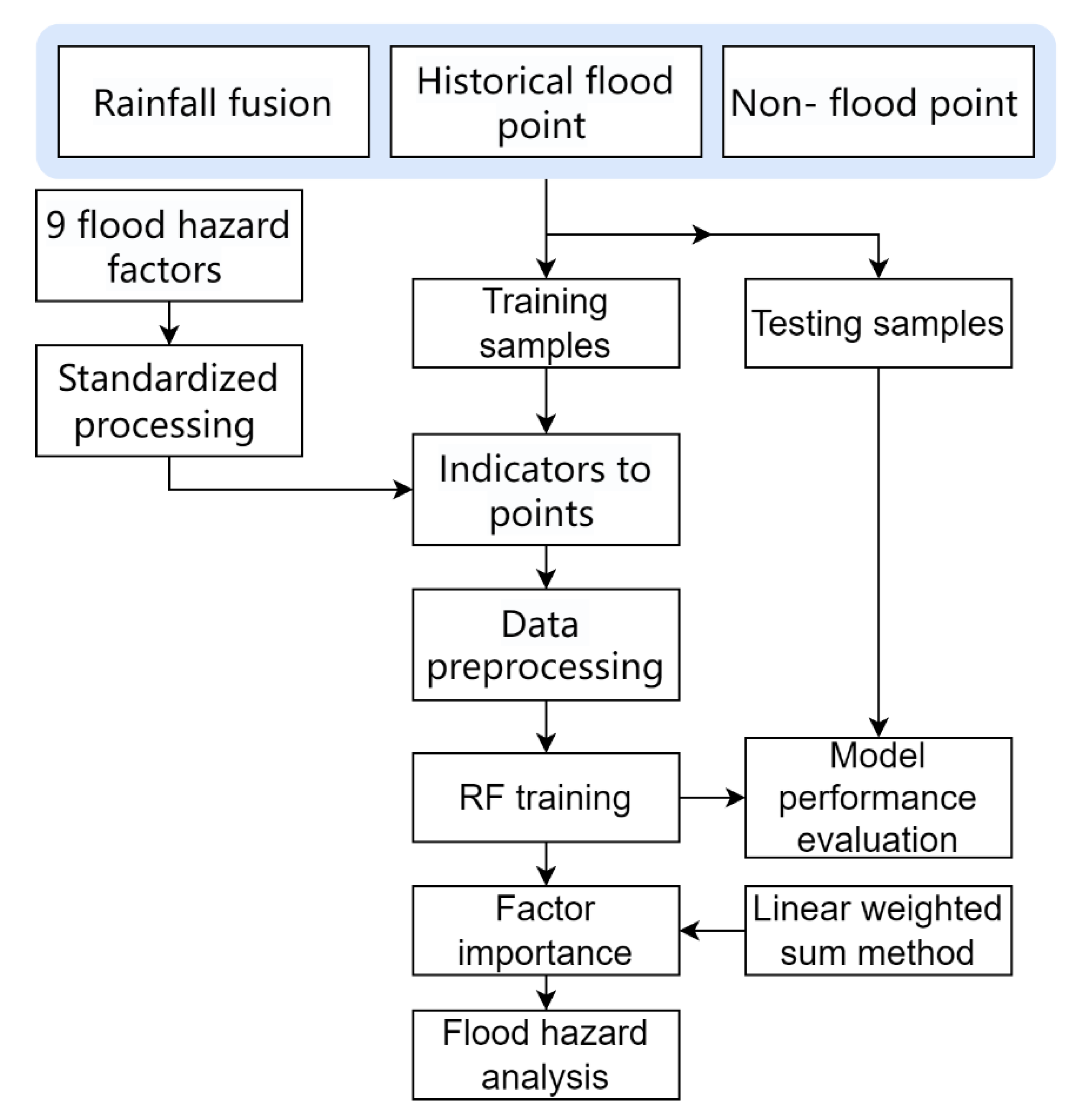
Figure 3 shows the schematic diagram of the flood hazard analysis system in this study. Firstly, nine flood hazard factors are chosen and calculated. Secondly, four rainfall fusion methods are applied to fuse the TRMM 3B42 and gauge rainfall. Thirdly, random forest (RF), linear weighted sum method (LWS), and certain factor (CF) model are used to form a system to conduct the flood hazard analysis. Finally, fused rainfall and flood hazard analysis results are comprehensively evaluated.

3.1. Flood Hazard Factors Calculation

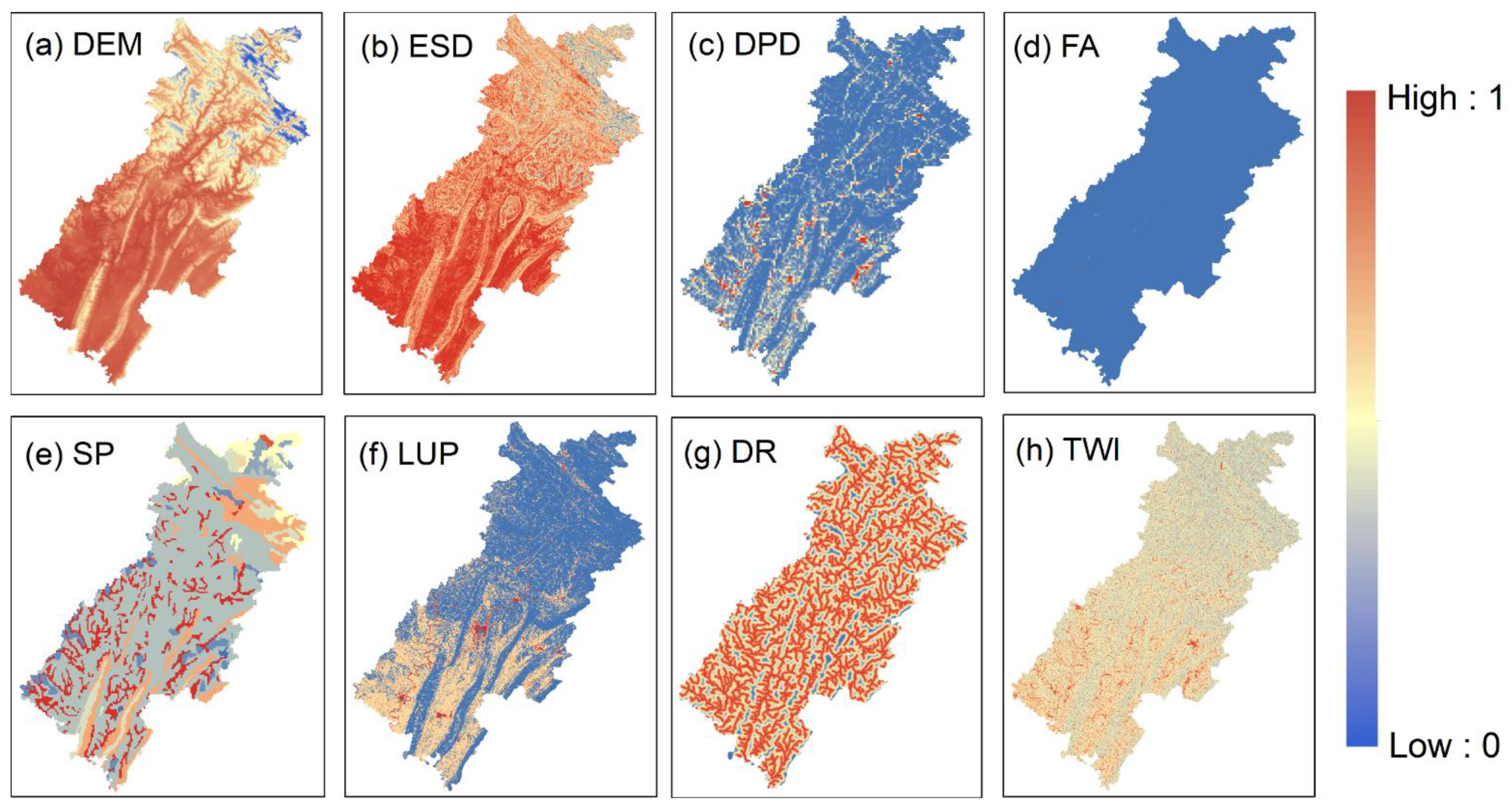
The appropriate factors are critical for flood hazard analysis [65], and nine representative ones are chosen for this study, as shown in Table 1, according to the previous studies [59,66,67,68]. They are three topographic factors: Digital Elevation Model (DEM), Elevation Standard Deviation (ESD), and Depression Point Density (DPD); five hydrological factors: Flow Accumulation (FA), Soil Permeability (SP), Land Use (LU), Distance to River (DR), and Topographic Wetness Index (TWI); and one precipitating factor: maximum precipitation (MAP), of which 3, 6, 9, and 12 h are denoted as MAP-3 h, MAP-6 h, MAP-9 h, and MAP-12 h, respectively. The spatial distribution of these factors, except MAP, in this study is shown in Figure 4, and the calculations are described in the following contents.
(1) Topographic factors
DEM (m): the flow trends run from areas with higher altitudes to lower areas, making the higher probability of flood events for flat terrain. The DEM data used in this study comes from Geospatial Data Cloud (https://www.gscloud.cn (accessed on 6 August 2021)), with a spatial resolution of 30 m.
ESD: this factor can sensitively reflect the study area’s topographic fluctuation. The areas with smaller ESD values are less conducive to the flow, which could easily form waterlogging. Thus, it is a negative factor for flood hazard. The ESD values are calculated within a circle of 0.25° radius for each grid by the Spatial Analyst Tools in ArcGIS software, based on the DEM map, and the formula is:
E S D = 1 n c 1 i C ( z i z ¯ ) 2
where C is the circle with a radius of 0.25° corresponding to each grid; i is the grid within the circle C; zi and z ¯ , respectively, represent the elevation value of the i-th grid and the mean elevation of all grids within the circle C; and nc is the number of grids within the circle C.
DPD: this can intuitively reflect the degree of depression filling in the region. According to the definition of depression, the greater DPD is, the higher flood hazard is. We collected the DPD map of Dazhou City by using ArcGIS Spatial Analyst Tools to process DEM data, and the formula is as follows:
D P D = n i S i
where ni is the number of depressions in the i-th grid; Si is the area of this grid.
(2) Hydrological factors
FA: this refers to the accumulation of surface runoff in each grid. The greater FA means more accumulated surface runoff, so it is easier to form waterlogging. Accordingly, FA has a positive effect on flood hazard. FA map was obtained through the flow direction and accumulation calculation with ArcGIS Hydrology Analyst Tools.
SP: soil permeability of various soil textures is coded by numbers, which come from Harmonized World Soil Database (HWSD) [69], as shown in Table 2. A larger number for SP indicates the more potent the soil infiltration capacity is, and the less likely it is to accumulate water.
LU: there are apparent differences in runoff conditions under different land uses, which are often distinguished by runoff coefficients ranging from 0 to 1. The values of the positive indicator LU in humid areas are always greater than those in arid areas. This is according to “Standard for Design of Building Water Supply and Drainage” (GB 50015-2019) [70] and “Standard for Design of Outdoor Wastewater Engineering” (GB50014-2021) [71], as shown in Table 3.
DR: the water level in the river channel is generally high during the flood season, and the heavy rainfall causes it to overflow the embankment, leading to floods. The areas close to the river are susceptible to flooding and have a high degree of danger, so the DR has a negative effect on the flood hazard assessment. In this paper, we applied ArcGIS to extract the river channels in the study area and used the Euclidean distance method to calculate the distance from each grid to the rivers.
TWI: this can clearly show the change of the runoff coefficient under different terrain conditions and provide an important way to explore the spatial distribution of soil moisture. The greater TWI is, the higher the surface runoff of the grid, and the more prone it is to floods. Thus, TWI is a positive factor. We obtained the TWI map, according to its definition formula, through the grid calculator tool in ArcGIS:
T W I = ln ( α tan β )
where α is the catchment area corresponding to the unit contour length in each grid; β is the slope.
(3) Precipitating factors
MAP: heavy rainfall in a short period is the most crucial factor in triggering flooding. This study set up four rainfall duration cases, including 3 h, 6 h, 9 h, and 12 h. MAP-3 h, MAP-6 h, MAP-9 h, and MAP-12 h, accordingly, are selected as flood-inducing factors for the corresponding duration. Specifically, MAP-3 h was the average of the maximum rainfall from 1986 to 2019 (the rainfall data from 1986 to 1997 is observed, the part from 1998 to 2012 is the fusion rainfall in this study, and the data from 2013 to 2019 is taken from the TRMM 3B42 dataset). MAP-6 h, MAP-9 h, and MAP-12 h are obtained by accumulating MAP-3 h. In order to avoid the situation where the maximum value of some factors affects the final superposition results of all factors in the flood hazard analysis, the factors mentioned above are separately standardized to [0,1].

3.2. Rainfall Data Fusion Methods

This study applies four frequently used fusion methods, LR, KF, GWR, and OI, to fuse the TRMM 3B42 and the observed rainfall.

3.2.1. Linear Regression (LR) Method

LR is a regression analysis method that uses the least squares function to establish a relationship model between one or more independent variables and dependent ones [72,73]. Accordingly, in the linear fusion experiment of TRMM 3B42 and gauge rainfall, we, firstly, conduct a correlation analysis between the two datasets to establish their linear regression model. Then, the coefficients in the regression model are obtained by the least squares method to correct the TRMM 3B42 in Dazhou City. The basic steps are as follows.
Assuming that the linear regression equation between TRMM 3B42 and gauge rainfall is:
P g = A * P s + B
A = r σ P g σ P s , B = P ¯ g A * P ¯ s
Combining Equations (4) and (5), we obtain:
P g P ¯ g = r σ P g σ P s ( P s P ¯ s )
where A and B are regression coefficients; Pg is gauge rainfall data; Ps is TRMM 3B42 in the corresponding grid; r is the correlation coefficient; P ¯ g and P ¯ s are the mean of the gauge and TRMM series, respectively; and σPg and σPs are the mean square errors of them. The calculation formulas are as follows:
r = i = 1 n ( P s i P ¯ s ) ( P g i P ¯ g ) i = 1 n ( P s i P ¯ s ) 2 ( P g i P ¯ g ) 2
σ P g = i = 1 n ( P g i P ¯ g ) 2 n 1
σ P s = i = 1 n ( P s i P ¯ s ) 2 n 1
where Pgi is the gauge rainfall of the i-th ground station; Psi is TRMM 3B42 data of the grid corresponding to the i-th ground station; and n is the number of ground stations.

3.2.2. Kalman Filter (KF) Method

KF is an optimal recursive data processing algorithm, which has been widely used in various fields, such as image recognition, fingerprint recognition, and the control of intelligent robot systems [74,75]. KF method assumes that the optimal estimation of the point is related to the previous point and uses the statistical estimation method to obtain the optimal estimation by analogy. The advantage of KF is that it requires little memory and runs efficiently. The time update equations in KF can be expressed as follows:
x ^ k ¯ = A x ^ k 1 + B u k + w k 1
where x ^ k 1 is the posterior state estimate of the point k−1; x ^ k ¯ is the prior state estimate of the point k; wk is the process noise and is assumed to have zero mean value; A is the state transition matrix; B is the matrix that transforms the input into a state; and uk−1 is measurement noise.
P k ¯ = A P k 1 A T + Q
where P k 1 is the posterior covariance estimate of the point k−1; P k ¯ is the prior covariance estimate of the point k; and Q is the covariance of process excitation noise.
As for the KF measurement update equations:
K k = P k ¯ H T H P k ¯ H T + R
x ^ k = x ^ k ¯ + K k ( z k H x ^ k ¯ )
P k = ( I K k H ) P k ¯
where H is the transformation matrix from state variables to observations; R is the covariance of measurement noise; Kk is the filter gain matrix; x ^ k is the posterior state estimate of the point k; zk is the input of filtering, i.e., measured values; and P k is the posterior covariance estimate of the point k.

3.2.3. Geographically Weighted Regression (GWR) Method

GWR is a robust algorithm successfully used in fusing rainfall [56]. It assumes that the rainfall gauge Pg and the satellite precipitation Ps are set to measure a constant quantity:
P g = X + V g
P s = X + V s
where Vg and Vs are random errors existing in observation and detection; Vg ~ N(0, σg2); and Vs ~ N(0, σs2). Moreover, assuming that the estimated value X ^ of the actual rainfall X is linearly related to the Pg and Ps, X ^ is an unbiased estimate of X:
X ^ = w g P g + w s P s
where wg and ws are the weights of two rainfall data.
The estimated error X ˜ and its mean square error E ( X ˜ ) can be expressed as:
X ˜ = X X ^
E ( X ˜ ) = E [ X w g ( X + P g ) w s ( X + P s ) ] 2

3.2.4. Optimal Interpolation (OI) Method

Choosing a dataset as the optimal values’ background field is the OI method’s first step [76,77]. We selected satellite rainfall data with high spatial coverage and denoted it as F. The gauge rainfall is taken as the observation value due to the high accuracy, and we denoted it as O. Accordingly, the optimal rainfall, denoted as A, obtained by the optimal interpolation method can be expressed as:
A k = F k + i = 1 n W i ( O i F i )
where k is the efficient grids in the divided analysis range, which is the circles with a radius of 0.25°; Wi is the weight assigned to the estimation of the bias between the observations and the background values. The error variance of the optimal values at the analysis point k is:
E 2 = ( A k T k ) 2 ¯
where Tk is the actual rainfall of point k.
It is assumed that the errors of the observation and the initial background field are not correlated, that is:
( O i T i ) ( F j T j ) ¯ = 0
Combining Equations (20)–(22):
E 2 = ( σ k f ) 2 + i = 1 n j = 1 n W i W j ( τ i j f + τ i j o ) 2 ( i = 1 n W i τ i k f )
where ( σ k f ) 2 is the error variance of the initial background field; τ i j f = ( F i T i ) ( F j T j ) ¯ and τ i j o = ( O i T i ) ( O j T j ) ¯ are the error covariance of the initial background field and the observation filed, respectively.

3.3. Construction of Flood Hazard Evaluation System

3.3.1. Linear Weighted Sum (LWS) Method

As an evaluation function method, the LWS method assigns the corresponding weight coefficients to each target according to its importance and then performs optimization for its linear combination [78,79]. We applied the LWS method to construct the flood hazard analysis system in this study. The specific formula of the linear weighted sum method is:
y = i = 1 n w i x i
where y is the comprehensive evaluation value of the system or the object being evaluated; n is the number of factor variables; xi is the i-th factor; and wi is the corresponding weight coefficient.

3.3.2. Certain Factor (CF) Model

CF model is a probability function, first proposed by Shortliffe and Buchanan [80], to clarify the hierarchical state weights of various factors that affect the occurrence of an event [81,82]. It has been widely used in landslide-susceptibility zoning by combining it with GIS technology, and its formula is:
C F = P a P s P a ( 1 P s ) , P a P s P a P s P s ( 1 P a ) , P a < P s
where Pa is the conditional probability that an event (flood) occurs in the classification state a of the related factors. In practical applications, it is often expressed as the ratio of the number of flood occurrence points to the area of the classification state a. Ps is the probability of historical floods occurring in the study area; that is, the ratio of total flood disaster points to the area of the study area.
The value range of CF is [−1, 1]. CF > 0 means that the event has a high possibility of happening, and when CF < 0, it means that the event is less likely to happen. When CF = 1, this event must happen, whereas CF = −1 is the opposite. If CF = 0, it is impossible to judge whether the event has occurred.

3.3.3. Flood Hazard Analysis System

Random forest (RF) is a classification method that equips multiple decision trees for effective classification through ensemble learning [26,83,84]. In this study, the RF model with default hyperparameters was applied to obtain the weights of various factors. Then, the LWS method was used to construct a flood hazard analysis system, as shown in Figure 4. Specifically, several important parameters of the RF model and their default values in the scikit-learn Python library are the number of decision trees (n_estimators = 100), the minimum number of samples required to split an internal node (min_samples_split = 2), the maximum depth of each decision tree (max_depth = none, i.e., the nodes are expanded until all leaves are pure or until all leaves contain less than min_samples_split samples), and the number of features to consider when looking for the best split (max_features = ‘sqrt’, sqrt is the total number of features).
Moreover, the holdout validation method was used to evaluate the analytical performance of the RF model. As for the flood disaster data in Dazhou City, we extracted 2254 historical flood occurrence points (Figure 2), which are divided into 676 (30%) test samples and 1578 (70%) training samples. The training of the RF classification model requires at least two or more classification attributes. Accordingly, 2254 non-flood occurrence points were randomly generated in the study area through ArcGIS and divided into 676 test samples and 1578 training samples. Then, the CF value of the chosen factors at each point is obtained by using the CF model. Moreover, the RF model established in Python is used to classify the flood hazard factors to obtain the weight of each factor under the four rainfall duration setups (3 h, 6 h, 9 h, and 12 h). Finally, the flood hazard analysis system in ArcGIS is established, dividing the study area’s grids into five zones, low, sub-low, medium, sub-high, and high, using the Natural Break Method.

3.4. Statistical Metrics

For the evaluation of the accuracy and overall errors of the fusion results of three-hour rainfall data from 1998 to 2012, three popular metrics, correlation coefficient (R), mean bias (MBIAS), and root-mean-square error (RMSE), are adopted in this paper:
R = i = 1 n ( P g , i P ¯ g ) ( P s , i P ¯ s ) i = 1 n ( P s , i P ¯ s ) 2 t = 1 n ( P g , i P ¯ g ) 2
M B I A S = i = 1 n ( P s , i P g , i ) n
R M S E = i = 1 n ( P s , i P g , i ) 2 n
For the performance evaluation of the proposed flood hazard system, the probability of corrected analysis (PCA), refers to the ratio of correctly detected floods to total observed floods:
P C A = N c N t
where Nt is the number of all sample points; and Nc is the number of points with correct analysis results.

4. Results

4.1. Performance Evaluation of Four Fusion Methods

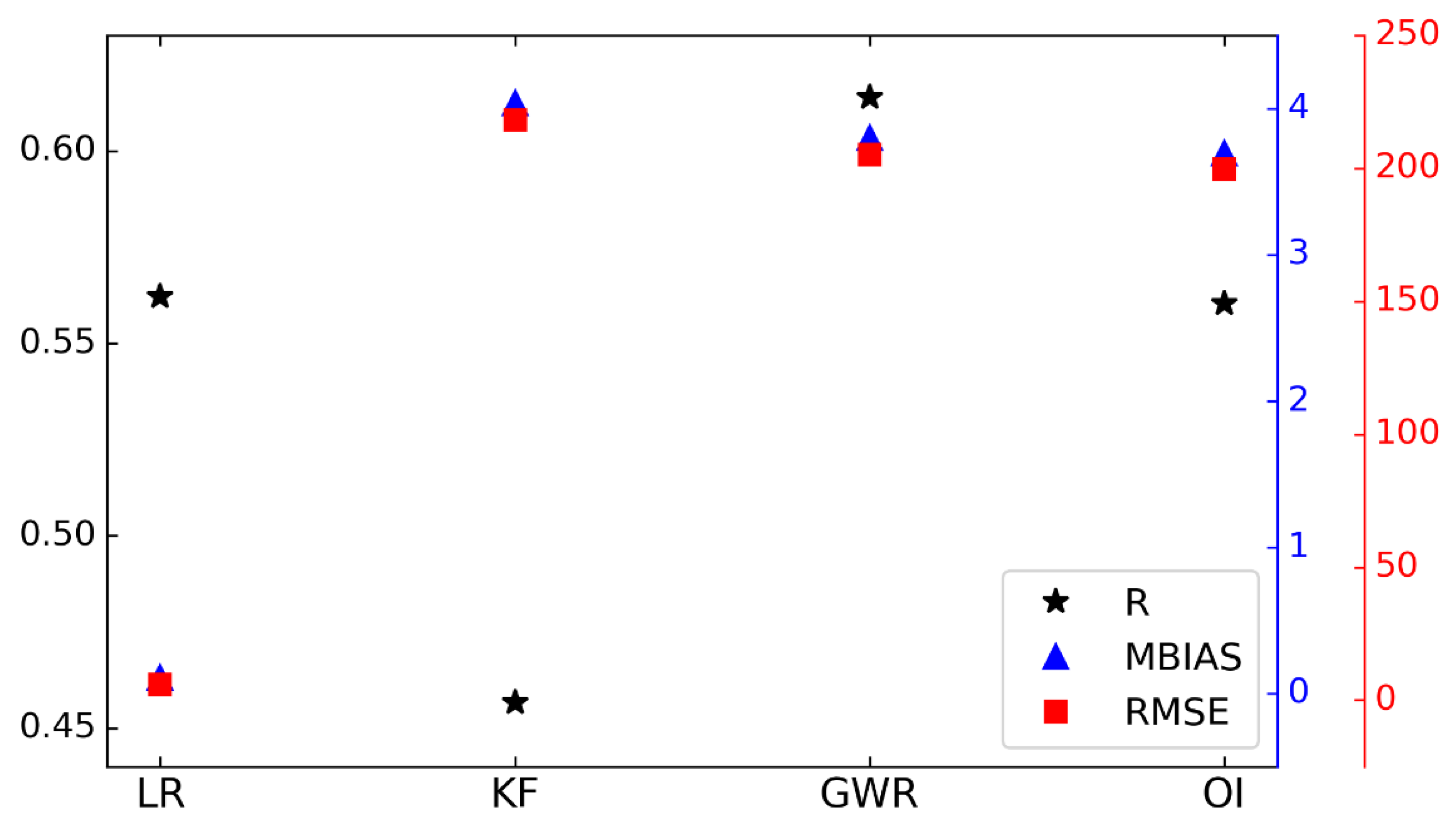
Figure 5 shows the performance of the four fusion methods (LR, KF, GWR, and OI) in the fusion experiment of three-hour TRMM 3B42 and gauge rainfall from 1998 to 2012. It can be found that the KF method has the lowest R-value, only 0.46. It means that the fusion rainfall obtained by this method has the worst correction with the observations. The GWR method has the highest R of 0.62, which is slightly better than the LR and OI, with an R-value of 0.56. A previous study [59] validated that the TRMM 3B42 has an R of 0.2 in this area. Considering the MBIAS between the fusion rainfall from the four methods and the gauge rainfall, the LR method has the lowest value, 0.20. However, the other three are obviously inferior due to the higher MBIAS, which is around 4.00. The MBIAS value of the OI method is slightly lower than that of GWR, and the highest value is from KF. As for the RMSE, it has a similar performance to the MBIAS. LR obtains the fusion rainfall with the lowest RMSE (0.10). KF, GWR, and OI have significantly higher RMSE, about 220. Therefore, the LR method is chosen for fusing the satellite and gauge rainfall in Dazhou City.
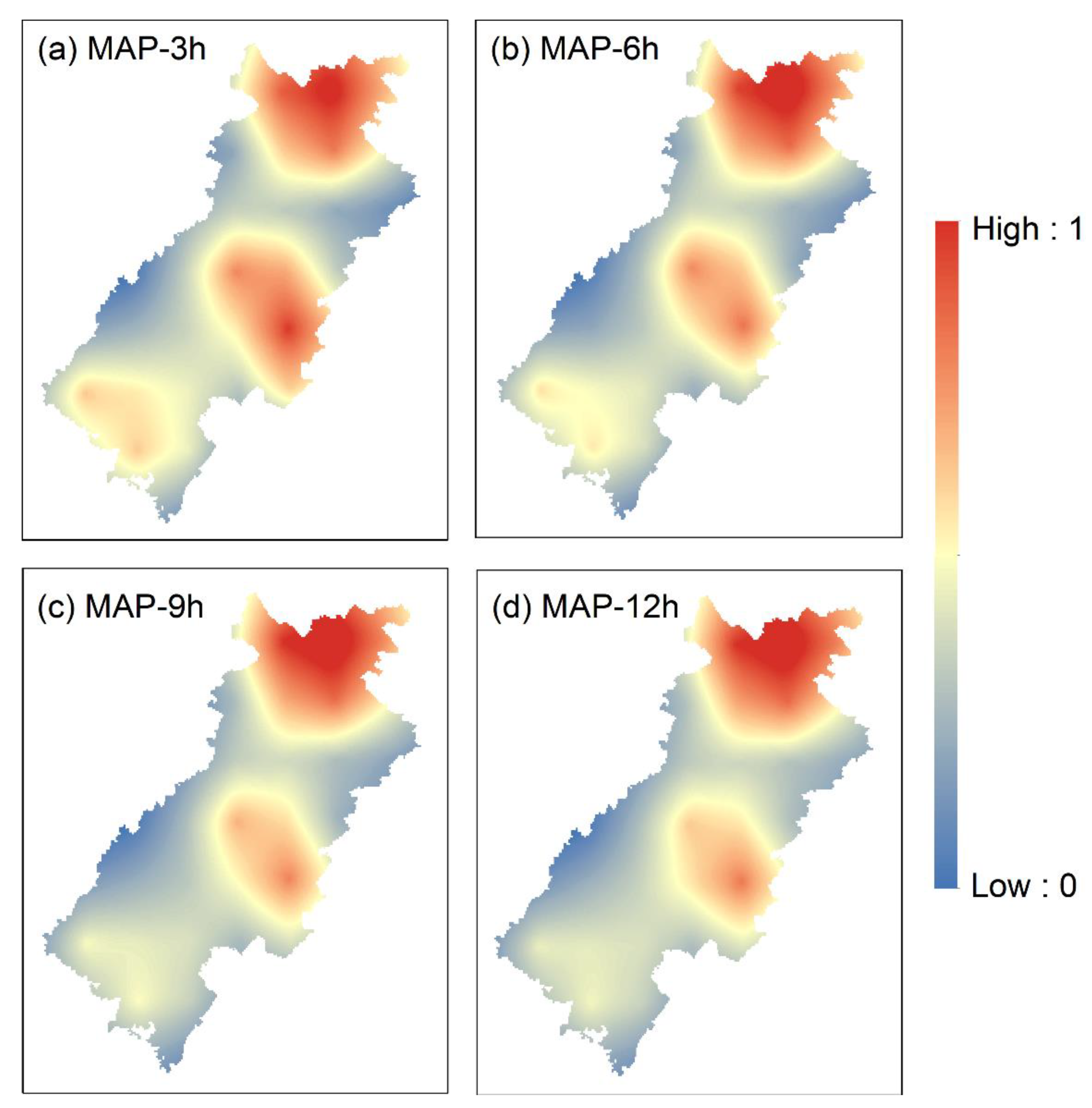
As described in Section 2.2.1, four precipitating factors, MAP-3 h, MAP-6 h, MAP-9 h, and MAP-12 h, are obtained based on the fusion rainfall using the LR method. The spatial distribution of MAP-3 h is shown in Figure 6a, and MAP-6 h, MAP-9 h, and MAP-12 h, acquired by accumulating MAP-3 h, are shown in Figure 6b–d. It can be found that the maximum precipitation during the various time scales in Dazhou City is mainly concentrated in northern Wanyuan and central Xuanhan. The highest MAPs are always in northern Wanyuan. The southern Qu and Dazhu also have relatively high MAP, gradually becoming less significant as the time scale increases.

4.2. Factor Weight Values from RF Model

As for the performance of the flood risk analysis system (Section 3.2) in designing the weights for the nine factors (Section 2.2.2), the PCA values (Equation (29)) during the training period under four rainfall durations, i.e., 3 h, 6 h, 9 h, and 12 h, are 0.824, 0.816, 0.818, and 0.821, respectively. During the testing period, the PCA values are 0.802, 0.805, 0.811, and 0.789, respectively, with acceptable reductions. Overall, the system’s performance is satisfactory, and, accordingly, the weight analysis results are considered reasonable.
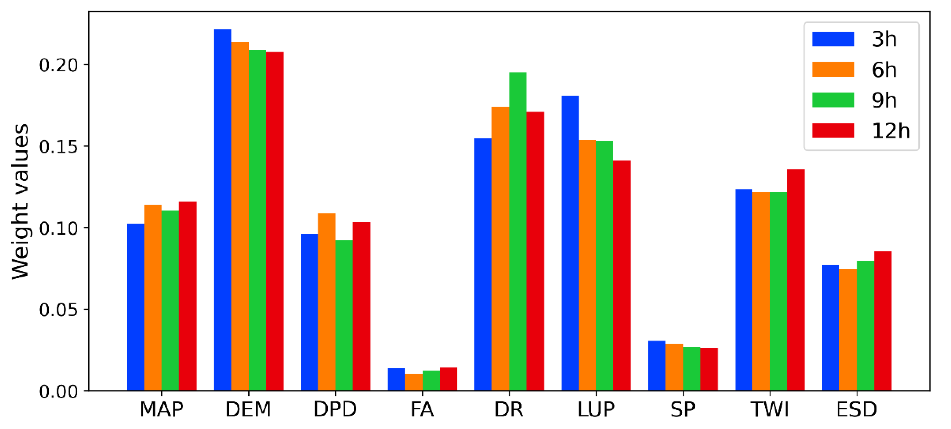
The weight values of the nine flood hazard factors under the four rainfall durations obtained by the proposed flood hazard analysis system are shown in Figure 7. We can see that all the highest weights are assigned to DEM in the four duration cases, and it is the only one of the nine factors with an importance ratio that exceeds 20%. Thus, DEM is the factor that contributes the most to the flood hazard. Two factors that contribute more to the hazard of flooding, followed by DEM, are DR and LU, and the importance of DR is slightly higher than that of LU. In descending order of importance, the flood hazard factors with a weight ratio of about 10% are TWI, MAP, DPD, and ESD. Their contribution to the hazard of flooding is moderate. The weights of SP and FA are relatively low, especially those of FA.

4.3. Flood Hazard Analysis

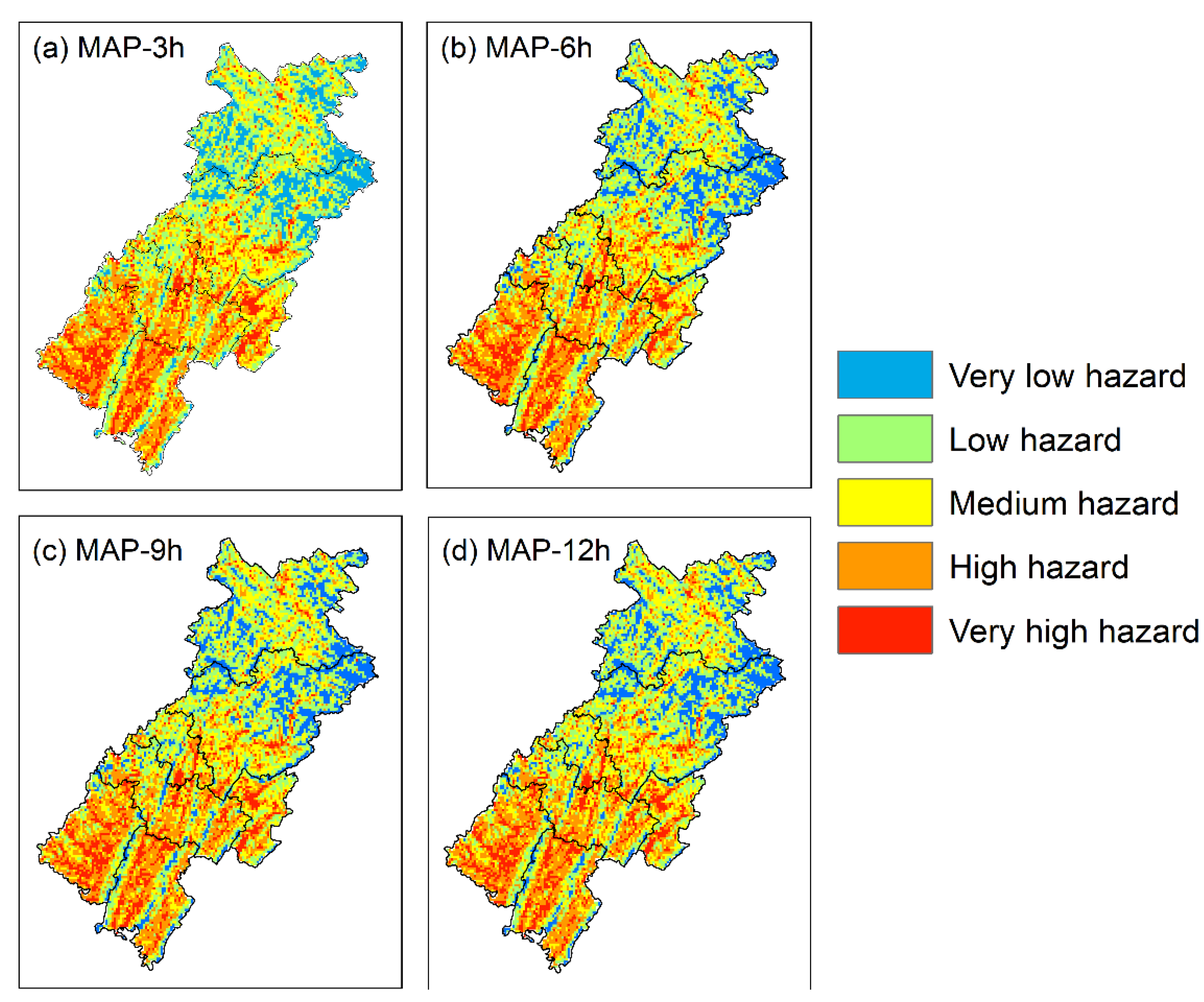
Figure 8 shows the spatial distribution of flood hazard in the 3 h, 6 h, 9 h, and 12 h rainfall duration cases in Dazhou City, based on the hazard index value obtained by the LWS method, with the weight value of each factor obtained above. The studied areas with high flood hazard are mainly concentrated in the south of Xuanhan, including the southern part of Tongchuan, the western part of Kaijiang, the eastern part of Qu, and the central and eastern parts of Dazhu. The relatively dangerous areas with sub-high hazard are mainly distributed in the south of Dachuan, such as the western part of Kaijiang, the southern part of Dachuan, the southeastern part of Qu, and the central and southeastern parts of Dazhu. However, the moderately dangerous areas are scattered, such as Tongchuan, the central part of Wanyuan, the southern part of Xuanhan, the mountainous areas at the junction of Qu and Dazhu, and the western part of Dachuan. The remaining areas belong to safe and relatively safe areas, mainly distributed in the eastern, northern, and northeastern parts of Xuanhan and the western and eastern parts of Wanyuan. Moreover, with increased rainfall duration, the area and distribution of each hazard zone did not change significantly. Comparing the results of flood hazard distribution with various flood factors, it is not difficult to realize that the areas with high flood hazard tend to be closer to rivers, with lower terrain and land use with larger runoff coefficients. This is well consistent with the weight assignment of each factor.
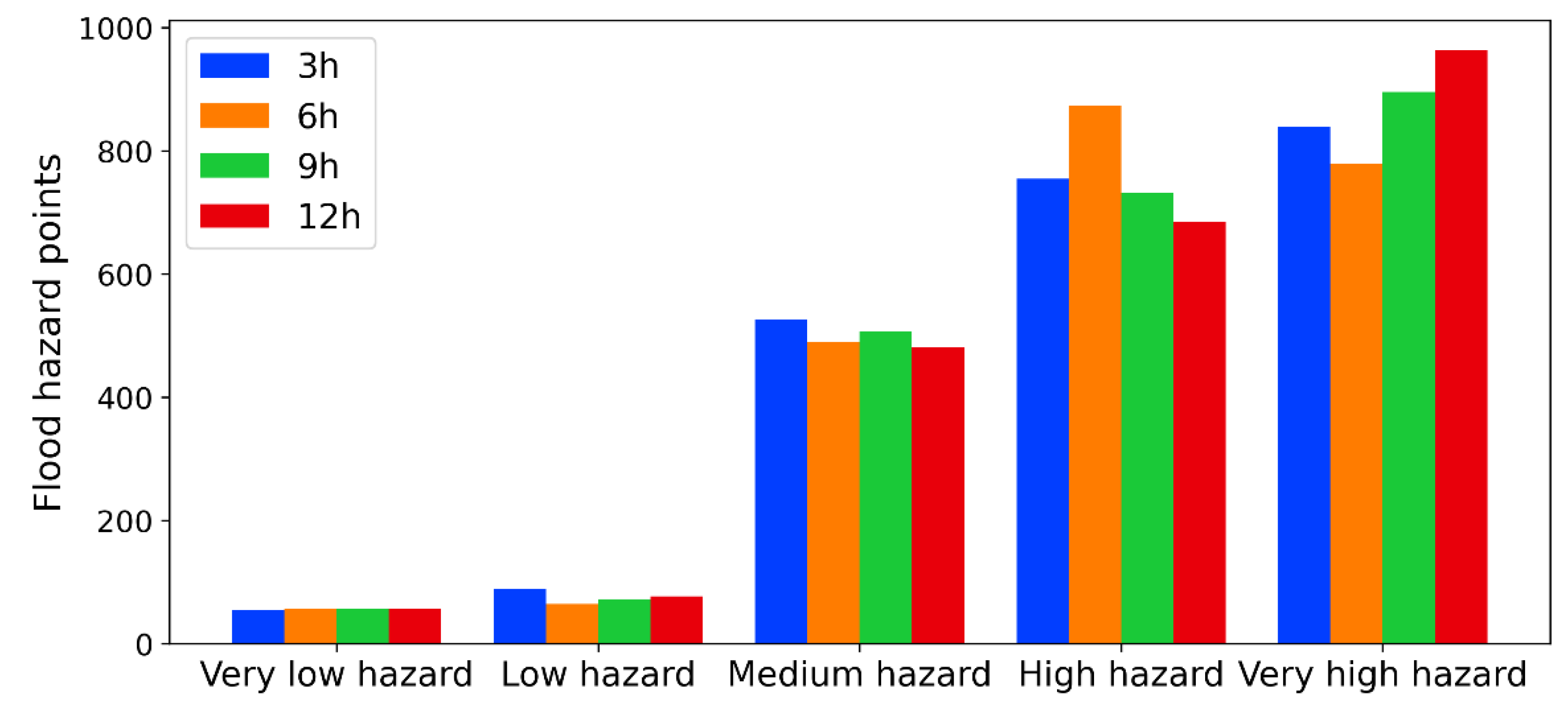
To verify the rationality of flood hazard analysis results of the proposed system, we counted the number of the collected historical flood points distributed in five flood hazard zones, as shown in Figure 9. It can be found that there is little difference in the numbers of historical flood points located in five hazard zones in the four rainfall duration cases. A similar performance is that the number of historical flood points in the high-hazard zone is the largest, accounting for more than 34%. It is followed by the sub-high hazard zone, about 30% or more. This means that approximately 70% or more of the flood points are distributed in relatively high flood hazard zones. More than 93% of flood points are located in the medium-hazard area and above. The low and sub-low hazard zones have the fewest historical flood points at less than 7%.

5. Discussion

(1) Applicability of the rainfall fusion method
Since rainfall has great spatial and temporal variability, it has strong regional characteristics [85,86]. Whether the method used in this paper is applicable in other regions still needs further experimental verification. Moreover, the impact of ground observation density on the performance of the fusion method remains to be verified. In addition, this study only selected two rainfall datasets, which may lead to uncertainties in the fused results. Although the liner regression method is proved the best among the four fusion methods, it needs further experimental verification when we apply the fusion methods to other areas with different gauge distribution and rainfall datasets.
(2) Impact of rainfall duration
In several cases with different rainfall durations, it can be found that, with the increase in rainfall duration, both the weight values of MAP and DR show an increasing trend, while that of DEM, LU, and SP are decreasing. There are no apparent changes in the weights of other factors. These indicate that the changes in precipitation duration impact the weights of flood hazard factors, but the limited impact makes it not decisive for the division of factor importance. These finds are consistent with other studies [87,88], which indicate that the impact of the rainfall duration factor on the flood hazard analysis needs to be further addressed.
(3) Performance of the flood hazard analysis
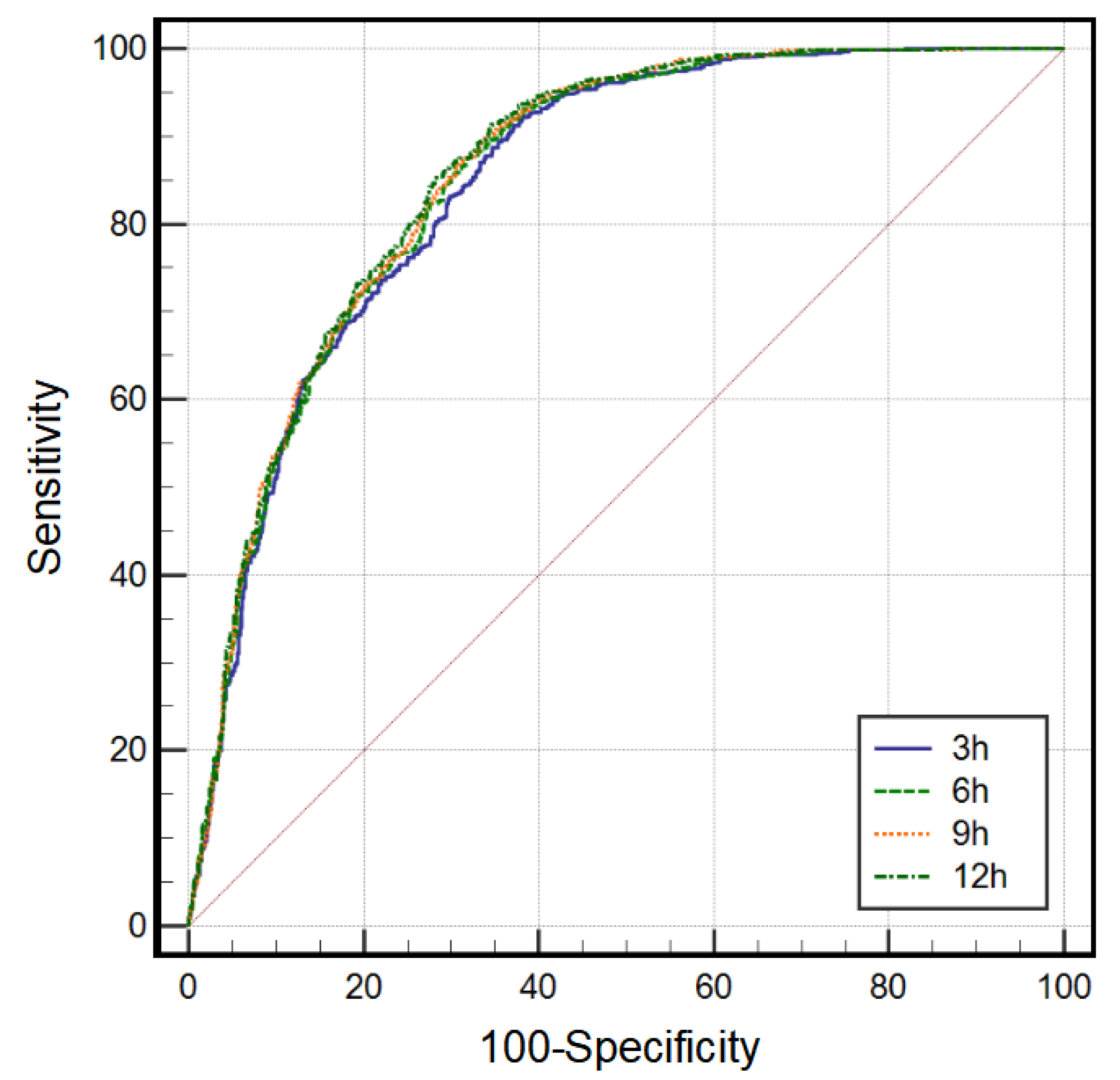
We plotted the Receiver Operating Characteristic (ROC) curves of the flood hazard in the four rainfall duration cases (3 h, 6 h, 9 h, and 12 h), as shown in Figure 10. Calculating the area under the ROC curves (AUC) of various cases, and they are about 0.847 (0.835–0.858), 0.853 (0.841–0.864), 0.856 (0.845–0.868) and 0.859 (0.847–0.870). All AUC values are in the range of 0.7–0.9, indicating that the proposed system has a great performance in predicting the flood hazard and can be used to predict whether flooding will occur in the study area.
(4) Insights for the management of flood hazard
Several previous studies have addressed an end-to-end approach to realize the scientific problem to the practical response, such as early warning [89,90], evacuation planning [91,92,93], and flood memory understanding [94]. As the results show in Figure 8, the flood hazard areas in Dazhou are mainly concentrated near the river and the northwest of Wanyuan. The lower dangerous areas are concentrated near the Qu River in Qu County and the area near the river in Dazhu. The safe areas are mainly distributed in the east, south, and southwest of Wanyuan, most of Xuanhan, and the north of Tongchuan. It could provide managerial information for city planning, which can reduce the hazard for the people and buildings to some extent. However, the resolution of this hazard map and the hazard analysis results of this study still need to be improved in future work.
In short, the flood hazard analysis system proposed in this paper has a satisfactory application in Dazhou City and is of great significance to flood hazard assessment and management.
(5) Limitation of this study
Firstly, the satellite rainfall data used in this study has a spatial scale of 0.25° due to the chosen period (1998–2019) not having finer datasets such as Integrated Multi-satellitE Retrievals for GPM (IMERG) or Global Satellite Mapping of Precipitation (GSMaP) [95]. The application effect on a high-resolution spatial scale needs to be further tested and analyzed in future work. In addition, to improve the ability to detect and predict flood disasters, conducting the rainfall fusion at a finer temporal resolution, such as half an hour or one hour, would be necessary.
Secondly, we mainly optimize and improve the rainfall factor, one of the nine selected flood hazard factors, to improve the accuracy of hazard analysis. However, this paper does not consider risk factors related to social and economic factors, which should be addressed in our future research.

6. Conclusions

For the flood hazard analysis, high data quality and the reasonable weight assignment of the relevant factors are very important. In this paper, taking Dazhou City as an experiment case, we obtained the fused rainfall data with higher precision by applying four rainfall fusion methods. Then, it was regarded as one of the important factors of the flood hazard analysis. The following conclusions can be drawn from this study:
(1)
For the fusion experiment of three-hour TRMM 3B42 and gauge rainfall from 1998 to 2012 in Dazhou City, the LR method has an outstanding performance, with the lowest MBIAS (0.20) and RMSE (0.10) and an acceptable R (0.56).
(2)
The RF model has a great performance in clarifying the weights of the nine hazard indicators, which is reflected in the fact that the PCA values of the cases corresponding to four rainfall durations, i.e., 3 h, 6 h, 9 h, and 12 h, which are all greater than 0.80 during the training period and are maintained at about 0.8 during the testing period. In addition, the most critical flood hazard factor is DEM (topography), followed by DR, while the least important one is FA.
(3)
The distribution of the flood hazard in Dazhou City, obtained by the proposed system using the higher-precision fusion rainfall and other eight flood indicators, is reasonable. More than 70% of historical flood points were in high and sub-high hazard zones, and the areas under the ROC curves were all within an acceptable range, 0.7–0.9, which further reflects the reliability of the flood hazard analysis results.
This paper optimizes and improves the quality of the rainfall, a precipitating factor, to improve the accuracy of the flood hazard analysis. In addition, a reasonable and effective flood hazard analysis system is proposed, to contribute to flood disaster assessment and management, especially for data-sparse areas. Moreover, the results of this paper can provide profound information for high-resolution flood risk assessment and management in Dazhou City in future work.

Author Contributions

Conceptualization, L.Z. and X.L.; methodology, L.L. and L.Z.; software, L.L. and X.S.; validation, L.L., X.L. and L.Z.; formal analysis, L.L., T.A., X.L. and L.Z.; investigation, X.L. and X.S.; data curation, X.L. and X.S.; writing—original draft preparation, L.L. and X.L.; writing—review and editing, L.Z.; visualization, X.L.; supervision, L.Z. and T.A.; funding acquisition, T.A. All authors have read and agreed to the published version of the manuscript.

Funding

This research was funded by the Regional Innovation Cooperation Program, grant number: 2020YFQ0013; Key R&D Project from the Science and Technology Department of Sichuan Province, grant number: 2021YFS028; and Key R&D Project from the Science and Technology Department of Tibet, grant number: XZ202101ZY0007G.

Institutional Review Board Statement

Not applicable.

Informed Consent Statement

Not applicable.

Data Availability Statement

Not applicable.

Acknowledgments

We gratefully acknowledge the anonymous reviewers for their comments and suggestions that improved this manuscript.

Conflicts of Interest

The authors declare no conflict of interest.

References

  1. Blais, E. Floods in a changing climate: Risk management. Can. Water Resour. J. Rev. Can. Des Ressour. Hydr. 2014, 39, 375–376. [Google Scholar] [CrossRef]
  2. Jongman, B.; Winsemius, H.C.; Aerts, J.C.J.H.; Coughlan De Perez, E.; van Aalst, M.K.; Kron, W.; Ward, P.J. Declining vulnerability to river floods and the global benefits of adaptation. Proc. Natl. Acad. Sci. USA 2015, 112, E2271–E2280. [Google Scholar] [CrossRef] [PubMed]
  3. Hirabayashi, Y.; Mahendran, R.; Koirala, S.; Konoshima, L.; Yamazaki, D.; Watanabe, S.; Kim, H.; Kanae, S. Global flood risk under climate change. Nat. Clim. Chang. 2013, 3, 816–821. [Google Scholar] [CrossRef]
  4. Tanoue, M.; Hirabayashi, Y.; Ikeuchi, H. Global-scale river flood vulnerability in the last 50 years. Sci. Rep.-UK 2016, 6, 36021. [Google Scholar] [CrossRef] [PubMed]
  5. Yang, K.; Chen, T.; Ao, T.; Zhang, X.; Zhou, L.; Gao, D. Response of runoff in the upper reaches of the Minjiang River to climate change. J. Water Clim. Chang. 2022, 13, 260–273. [Google Scholar] [CrossRef]
  6. Brody, S.D.; Zahran, S.; Highfield, W.E.; Grover, H.; Vedlitz, A. Identifying the impact of the built environment on flood damage in Texas. Disasters 2008, 32, 1–18. [Google Scholar] [CrossRef] [PubMed]
  7. EM-DAT: The OFDA/CRED International Disaster Database, Université Catholique de Louvain, Brussels, Bel. Data Version: v11.08, 2010. Available online: http://www.emdat.be/ (accessed on 6 August 2021).
  8. Nie, C.; Li, H.; Yang, L.; Wu, S.; Liu, Y.; Liao, Y. Spatial and temporal changes in flooding and the affecting factors in China. Nat. Hazards 2012, 61, 425–439. [Google Scholar] [CrossRef]
  9. Kundzewicz, Z.W.; Su, B.; Wang, Y.; Xia, J.; Huang, J.; Jiang, T. Flood risk and its reduction in China. Adv. Water Resour. 2019, 130, 37–45. [Google Scholar] [CrossRef]
  10. Liu Jianfen, Z.X.T.Z. Spatial distribution of flood hazards in China. J. Hohai Univ. Nat. Sci. Ed. 2004, 32, 614–617. [Google Scholar]
  11. Zhang, J.; Wang, T.; Ge, J. Assessing Vegetation Cover Dynamics Induced by Policy-Driven Ecological Restoration and Implication to Soil Erosion in Southern China. PLoS ONE 2015, 10, e131352. [Google Scholar] [CrossRef]
  12. Jia, H.; Chen, F.; Pan, D.; Du, E.; Wang, L.; Wang, N.; Yang, A. Flood risk management in the Yangtze River basin—Comparison of 1998 and 2020 events. Int. J. Disaster Risk Reduct. 2022, 68, 102724. [Google Scholar] [CrossRef]
  13. Song, M.L.; Du, Q.Q. Analysis and exploration of damage-reduction measures for flood disasters in China. Ann. Oper. Res. 2019, 283, 795–810. [Google Scholar] [CrossRef]
  14. Notaro, V.; Fontanazza, C.M.; La Loggia, G.; Freni, G. Flood frequency analysis for an urban watershed: Comparison between several statistical methodologies simulating synthetic rainfall events. J. Flood Risk Manag. 2018, 11, S559–S574. [Google Scholar] [CrossRef]
  15. Wang, J.; Liang, Z.; Hu, Y.; Wang, D. Modified weighted function method with the incorporation of historical floods into systematic sample for parameter estimation of Pearson type three distribution. J. Hydrol. 2015, 527, 958–966. [Google Scholar] [CrossRef]
  16. Bajracharya, S.R.; Khanal, N.R.; Nepal, P.; Rai, S.K.; Ghimire, P.K.; Pradhan, N.S. Community Assessment of Flood Risks and Early Warning System in Ratu Watershed, Koshi Basin, Nepal. Sustainability 2021, 13, 3577. [Google Scholar] [CrossRef]
  17. Gao, Y.; Zhao, S.; Deng, J.; Yu, Z.; Rahman, M. Flood assessment and early warning of the reoccurrence of river blockage at the Baige landslide. J. Geogr. Sci. 2021, 31, 1694–1712. [Google Scholar] [CrossRef]
  18. Su, X.; Shao, W.; Liu, J.; Jiang, Y.; Wang, K. Dynamic Assessment of the Impact of Flood Disaster on Economy and Population under Extreme Rainstorm Events. Remote Sens. 2021, 13, 3924. [Google Scholar] [CrossRef]
  19. Oddo, P.C.; Bolten, J.D. The Value of Near Real-Time Earth Observations for Improved Flood Disaster Response. Front. Environ. Sci. 2019, 7, 127. [Google Scholar] [CrossRef]
  20. Wang, Z.; Gao, Z. Dynamic monitoring of flood disaster based on remote sensing data cube. Nat. Hazards 2022. [Google Scholar] [CrossRef]
  21. Sun, T.; Li, R.; Deng, H.Y.; Li, X.T. Flood Disaster Monitoring and Evaluation System Based on GIS and Remote Sensing: Case Study in Hejiang River. Appl. Mech. Mater. 2012, 239–240, 560–564. [Google Scholar] [CrossRef]
  22. Ding, L.; Ma, L.; Li, L.; Liu, C.; Li, N.; Yang, Z.; Yao, Y.; Lu, H. A Survey of Remote Sensing and Geographic Information System Applications for Flash Floods. Remote Sens. 2021, 13, 1818. [Google Scholar] [CrossRef]
  23. Yang, T.; Xie, J.; Li, G.; Zhang, L.; Mou, N.; Wang, H.; Zhang, X.; Wang, X. Extracting Disaster-Related Location Information through Social Media to Assist Remote Sensing for Disaster Analysis: The Case of the Flood Disaster in the Yangtze River Basin in China in 2020. Remote Sens. 2022, 14, 1199. [Google Scholar] [CrossRef]
  24. Li, Q.; Jiang, X.; Liu, D. Analysis and modelling of flood risk assessment using information diffusion and artificial neural network. Water SA 2013, 39, 643–648. [Google Scholar] [CrossRef]
  25. Michielsen, A.; Kalantari, Z.; Lyon, S.W.; Liljegren, E. Predicting and communicating flood risk of transport infrastructure based on watershed characteristics. J. Environ. Manag. 2016, 182, 505–518. [Google Scholar] [CrossRef]
  26. Zhu, Z.; Zhang, Y. Flood disaster risk assessment based on random forest algorithm. Neural Comput. Appl. 2022, 34, 3443–3455. [Google Scholar] [CrossRef]
  27. Li, X.; Yan, D.; Wang, K.; Weng, B.; Qin, T.; Liu, S. Flood Risk Assessment of Global Watersheds Based on Multiple Machine Learning Models. Water 2019, 11, 1654. [Google Scholar] [CrossRef]
  28. Luu, C.; Von Meding, J.; Kanjanabootra, S. Assessing flood hazard using flood marks and analytic hierarchy process approach: A case study for the 2013 flood event in Quang Nam, Vietnam. Nat. Hazards 2018, 90, 1031–1050. [Google Scholar] [CrossRef]
  29. Yang, X.; Ding, J.; Hou, H. Application of a triangular fuzzy AHP approach for flood risk evaluation and response measures analysis. Nat. Hazards 2013, 68, 657–674. [Google Scholar] [CrossRef]
  30. Bachmann, D.; Schuttrumpf, H. Integrating the reliability of flood protection structures into catchment-based flood risk analysis. Hydrol. Wasserbewirts. 2014, 58, 168–177. [Google Scholar]
  31. Salleh, A.H.; S Ahamad, M.S. Flood risk map (case study in Kelantan). IOP Conf. Ser. Earth Environ. Sci. 2019, 244, 12019. [Google Scholar] [CrossRef]
  32. Jung, Y.; Shin, Y.; Jang, C.H.; Kum, D.; Kim, Y.S.; Lim, K.J.; Kim, H.B.; Park, T.S.; Lee, S.O. Estimation of flood risk index considering the regional flood characteristics: A case of South Korea. Paddy Water Environ. 2014, 12, 41–49. [Google Scholar] [CrossRef]
  33. Yalcin, G.; Akyurek, Z. Analysing flood vulnerable areas with multicriteria evaluation. In Proceedings of the 20th ISPRS Congress, Istanbul, Turkey, 12 July 2004; pp. 359–364. [Google Scholar]
  34. Stefanidis, S.; Stathis, D. Assessment of flood hazard based on natural and anthropogenic factors using analytic hierarchy process (AHP). Nat. Hazards 2013, 68, 569–585. [Google Scholar] [CrossRef]
  35. Ologunorisa, T.E. An Assessment of Flood Vulnerability Zones in the Niger Delta, Nigeria. Int. J. Environ. Stud. 2004, 61, 31–38. [Google Scholar] [CrossRef]
  36. Mansor, S.; Abu Shariah, M.; Billa, L.; Setiawan, I.; Jabar, F. Spatial technology for natural risk management. Disaster Prev. Manag. Int. J. 2004, 13, 364–373. [Google Scholar] [CrossRef]
  37. Sanyal, J.; Lu, X.X. GIS-based flood hazard mapping at different administrative scales: A case study in Gangetic West Bengal, India. Singap. J. Trop. Geogr. 2006, 27, 207–220. [Google Scholar] [CrossRef]
  38. Deo, R.C.; Byun, H.; Kim, G.; Adamowski, J.F. A real-time hourly water index for flood risk monitoring: Pilot studies in Brisbane, Australia, and Dobong Observatory, South Korea. Environ. Monit. Assess. 2018, 190, 450. [Google Scholar] [CrossRef]
  39. Kim, E.S.; Choi, H.I. A method of flood severity assessment for predicting local flood hazards in small ungauged catchments. Nat. Hazards 2015, 78, 2017–2033. [Google Scholar] [CrossRef]
  40. Skakun, S.; Kussul, N.; Shelestov, A.; Kussul, O. Flood Hazard and Flood Risk Assessment Using a Time Series of Satellite Images: A Case Study in Namibia. Risk Anal. 2014, 34, 1521–1537. [Google Scholar] [CrossRef]
  41. Trinh, M.X.; Molkenthin, F. Flood hazard mapping for data-scarce and ungauged coastal river basins using advanced hydrodynamic models, high temporal-spatial resolution remote sensing precipitation data, and satellite imageries. Nat. Hazards 2021, 109, 441–469. [Google Scholar] [CrossRef]
  42. Zhou, L.; Rasmy, M.; Takeuchi, K.; Koike, T.; Selvarajah, H.; Ao, T. Adequacy of Near Real-Time Satellite Precipitation Products in Driving Flood Discharge Simulation in the Fuji River Basin, Japan. Appl. Sci. 2021, 11, 1087. [Google Scholar] [CrossRef]
  43. Yufeng, R.; Guodong, L.; Li, Z.; Chunmin, Z. Risk evaluation of Chengdu’s flood hazard based on evidence theory and variable fuzzy sets theory. Trans. Chin. Soc. Agric. Eng. 2014, 30, 147–156. [Google Scholar]
  44. Reed, P.M.; Chaney, N.W.; Herman, J.D.; Ferringer, M.P.; Wood, E.F. Internationally coordinated multi-mission planning is now critical to sustain the space-based rainfall observations needed for managing floods globally. Environ. Res. Lett. 2015, 10, 24010. [Google Scholar] [CrossRef]
  45. Harris, A.; Rahman, S.; Hossain, F.; Yarborough, L.; Bagtzoglou, A.; Easson, G. Satellite-based Flood Modeling Using TRMM-based Rainfall Products. Sensors 2007, 7, 3416–3427. [Google Scholar] [CrossRef] [Green Version]
  46. Haile, A.T.; Tefera, F.T.; Rientjes, T. Flood forecasting in Niger-Benue basin using satellite and quantitative precipitation forecast data. Int. J. Appl. Earth Obs. 2016, 52, 475–484. [Google Scholar] [CrossRef]
  47. Shrestha, M.S.; Artan, G.A.; Bajracharya, S.R.; Gautam, D.K.; Tokar, S.A. Bias-adjusted satellite-based rainfall estimates for predicting floods: Narayani Basin. J. Flood Risk Manag. 2011, 4, 360–373. [Google Scholar] [CrossRef]
  48. Guzinski, R.; Nieto, H.; Sandholt, I.; Karamitilios, G. Modelling High-Resolution Actual Evapotranspiration through Sentinel-2 and Sentinel-3 Data Fusion. Remote Sens. 2020, 12, 1433. [Google Scholar] [CrossRef]
  49. Nourani, V.; Gökçekuş, H.; Gichamo, T. Ensemble data-driven rainfall-runoff modeling using multi-source satellite and gauge rainfall data input fusion. Earth Sci. Inform. 2021, 14, 1787–1808. [Google Scholar] [CrossRef]
  50. Zhou, L.; Koike, T.; Takeuchi, K.; Rasmy, M.; Onuma, K.; Ito, H.; Selvarajah, H.; Liu, L.; Li, X.; Ao, T. A study on availability of ground observations and its impacts on bias correction of satellite precipitation products and hydrologic simulation efficiency. J. Hydrol. 2022, 610, 127595. [Google Scholar] [CrossRef]
  51. Li, W.; Jiang, Q.; He, X.; Sun, H.; Sun, W.; Scaioni, M.; Chen, S.; Li, X.; Gao, J.; Hong, Y. Effective multi-satellite precipitation fusion procedure conditioned by gauge background fields over the Chinese mainland. J. Hydrol. 2022, 610, 127783. [Google Scholar] [CrossRef]
  52. Bi, S.; Bi, S.; Chen, D.; Pan, J.; Wang, J. A Double-Smoothing Algorithm for Integrating Satellite Precipitation Products in Areas with Sparsely Distributed In Situ Networks. ISPRS Int. J. Geo-Inf. 2017, 6, 28. [Google Scholar] [CrossRef]
  53. Turlapaty, A.C.; Younan, N.H.; Anantharaj, V. Precipitation data merging using general linear regression. In Proceedings of the 2009 IEEE International Geoscience and Remote Sensing Symposium, Cape Town, South Africa, 12–17 July 2009; Volume 3, pp. 259–262. [Google Scholar]
  54. Huang, Y.; Liu, H.; Yao, Y.; Ni, T.; Feng, Y. An Integrated Method of Multiradar Quantitative Precipitation Estimation Based on Cloud Classification and Dynamic Error Analysis. Adv. Meteorol. 2017, 2017, 1–6. [Google Scholar] [CrossRef]
  55. Chen, J.; Yong, B.; Ren, L.; Wang, W.; Chen, B.; Lin, J.; Yu, Z.; Li, N. Using a Kalman Filter to Assimilate TRMM-Based Real-Time Satellite Precipitation Estimates over Jinghe Basin, China. Remote Sens. 2016, 8, 899. [Google Scholar] [CrossRef]
  56. Chao, L.; Zhang, K.; Li, Z.; Zhu, Y.; Wang, J.; Yu, Z. Geographically weighted regression based methods for merging satellite and gauge precipitation. J. Hydrol. 2018, 558, 275–289. [Google Scholar] [CrossRef]
  57. Liu, S.; Yan, D.; Qin, T.; Weng, B.; Li, M. Correction of TRMM 3B42V7 Based on Linear Regression Models over China. Adv. Meteorol. 2016, 2016, 1–13. [Google Scholar] [CrossRef]
  58. Li, M.; Shao, Q. An improved statistical approach to merge satellite rainfall estimates and raingauge data. J. Hydrol. 2010, 385, 51–64. [Google Scholar] [CrossRef]
  59. Duan, Z.; Ren, Y.; Liu, X.; Lei, H.; Hua, X.; Shu, X.; Zhou, L. A comprehensive comparison of data fusion approaches to multi-source precipitation observations: A case study in Sichuan province, China. Environ. Monit. Assess. 2022, 194, 422. [Google Scholar] [CrossRef]
  60. Tropical Rainfall Measuring Mission (TRMM). TRMM (TMPA) Rainfall Estimate L3 3 hour 0.25 degree × 0.25 degree V7, Greenbelt, MD, Goddard Earth Sciences Data and Information Services Center (GES DISC), 2011. Available online: https://disc.gsfc.nasa.gov/datasets/TRMM_3B42_7/summary (accessed on 6 August 2021).
  61. Liu, Z.; Ostrenga, D.; Teng, W.; Kempler, S. Tropical Rainfall Measuring Mission (TRMM) Precipitation Data and Services for Research and Applications. B. Am. Meteorol. Soc. 2012, 93, 1317–1325. [Google Scholar] [CrossRef]
  62. Wu, H.; Yang, Q.; Liu, J.; Wang, G. A spatiotemporal deep fusion model for merging satellite and gauge precipitation in China. J. Hydrol. 2020, 584, 124664. [Google Scholar] [CrossRef]
  63. Shukla, K.; Kumar, P.; Mann, G.S.; Khare, M. Mapping spatial distribution of particulate matter using Kriging and Inverse Distance Weighting at supersites of megacity Delhi. Sustain. Cities Soc. 2020, 54, 101997. [Google Scholar] [CrossRef]
  64. Souza, T.J.; Medeiros, J.A.C.C.; Gonçalves, A.C.; Martinez, A.S. A method to identify an accidental control rod drop with inverse distance weighted interpolation. Ann. Nucl. Energy 2020, 145, 107462. [Google Scholar] [CrossRef]
  65. Bunmi Mudashiru, R.; Sabtu, N.; Abdullah, R.; Saleh, A.; Abustan, I. Optimality of flood influencing factors for flood hazard mapping: An evaluation of two multi-criteria decision-making methods. J. Hydrol. 2022, 612, 128055. [Google Scholar] [CrossRef]
  66. Baky, M.A.A.; Islam, M.; Paul, S. Flood Hazard, Vulnerability and Risk Assessment for Different Land Use Classes Using a Flow Model. Earth Syst. Environ. 2020, 4, 225–244. [Google Scholar] [CrossRef]
  67. Tingsanchali, T.; Karim, F. Flood-hazard assessment and risk-based zoning of a tropical flood plain: Case study of the Yom River, Thailand. Hydrol. Sci. J. 2010, 55, 145–161. [Google Scholar] [CrossRef]
  68. Lin, L.; Wu, Z.; Liang, Q. Urban flood susceptibility analysis using a GIS-based multi-criteria analysis framework. Nat. Hazards 2019, 97, 455–475. [Google Scholar] [CrossRef]
  69. Fischer, G.F.N.S. Global Agro-ecological Zones Assessment for Agriculture (GAEZ 2008); IIASA, Laxenburg, Austria and FAO: Rome, Italy, 2008. [Google Scholar]
  70. GB 50015-2019; Standard for Design of Building Water Supply and Drainage. Ministry of Housing and Urban-Rural Development. China Planning Press: Beijing, China, 2019.
  71. GB50014-2021; Standard for Design of Outdoor Wastewater Engineering. Ministry of Housing and Urban-Rural Development. China Planning Press: Beijing, China, 2021.
  72. Zhou, L.; Zhang, X.; Liu, L.; Chen, T.; Liu, X.; Ren, Y.; Zhang, H.; Li, X.; Ao, T. An approach to evaluate non-point source pollution in an ungauged basin: A case study in Xiao’anxi River Basin, China. Water Supply 2020, 20, 3646–3657. [Google Scholar] [CrossRef]
  73. Nada, D.; Bousbia-Salah, M.; Bettayeb, M. Multi-sensor Data Fusion for Wheelchair Position Estimation with Unscented Kalman Filter. Int. J. Autom. Comput. 2018, 15, 207–217. [Google Scholar] [CrossRef]
  74. Hosseinpour, A.; Dolcine, L.; Fuamba, M. Natural Flow Reconstruction Using Kalman Filter and Water Balance—Based Methods I: Theory. J. Hydrol. Eng. 2014, 19, 04014029. [Google Scholar] [CrossRef]
  75. Gan, Q.; Harris, C.J. Comparison of two measurement fusion methods for Kalman-filter-based multisensor data fusion. IEEE T. Aero. Elec. Sys. 2001, 37, 273–279. [Google Scholar] [CrossRef]
  76. Machado, P.L.; Oliveira, R.M.S.D.; Souza, W.C.B.; Araújo, R.C.F.; Tostes, M.E.L.; Gonçalves, C. An automatic methodology for obtaining optimum shape factors for the radial point interpolation method. J. Microw. Optoelectron. Electromagn. Appl. 2011, 10, 389–401. [Google Scholar] [CrossRef]
  77. Sun, W.; Wang, J.; Zhang, J.; Ma, Y.; Meng, J.; Yang, L.; Miao, J. A new global gridded sea surface temperature product constructed from infrared and microwave radiometer data using the optimum interpolation method. Acta Oceanol. Sin. 2018, 37, 41–49. [Google Scholar] [CrossRef]
  78. Gao, S.; Sun, H.; Liu, J.; Liu, W. Comprehensive audit evaluation and driving force analysis of various types of marine resources development. Environ. Dev. Sustain. 2022, 24, 4371–4386. [Google Scholar] [CrossRef]
  79. Wang, A.; Liu, J.; Wang, W. Flexibility-based improved model of multi-energy hubs using linear weighted sum algorithm. J. Renew. Sustain. Ener. 2018, 10, 15901. [Google Scholar] [CrossRef]
  80. Shortliffe, E.H.; Buchanan, B.G. A model of inexact reasoning in medicine. Math. Biosci. 1975, 23, 351–379. [Google Scholar] [CrossRef]
  81. Nahayo, L.; Kalisa, E.; Maniragaba, A.; Nshimiyimana, F.X. Comparison of analytical hierarchy process and certain factor models in landslide susceptibility mapping in Rwanda. Model. Earth Syst. Environ. 2019, 5, 885–895. [Google Scholar] [CrossRef]
  82. Rezaei, M.; Yazdani Noori, Z.; Dashti Barmaki, M. Land subsidence susceptibility mapping using Analytical Hierarchy Process (AHP) and Certain Factor (CF) models at Neyshabur plain, Iran. Geocarto Int. 2022, 37, 1465–1481. [Google Scholar] [CrossRef]
  83. Schoppa, L.; Disse, M.; Bachmair, S. Evaluating the performance of random forest for large-scale flood discharge simulation. J. Hydrol. 2020, 590, 125531. [Google Scholar] [CrossRef]
  84. Breiman, L. Random Forests. Mach. Learn 2001, 45, 5–32. [Google Scholar] [CrossRef]
  85. Liu, Y.; Li, Z.; Liu, Z.; Luo, Y. Impact of rainfall spatiotemporal variability and model structures on flood simulation in semi-arid regions. Stoch. Env. Res. Risk A 2021, 36, 785–809. [Google Scholar] [CrossRef]
  86. Khatakho, R.; Talchabhadel, R.; Thapa, B.R. Evaluation of different precipitation inputs on streamflow simulation in Himalayan River basin. J. Hydrol. 2021, 599, 126390. [Google Scholar] [CrossRef]
  87. Lompi, M.; Tamagnone, P.; Pacetti, T.; Morbidelli, R.; Caporali, E. Impacts of Rainfall Data Aggregation Time on Pluvial Flood Hazard in Urban Watersheds. Water 2022, 14, 544. [Google Scholar] [CrossRef]
  88. Wu, S.; Hsu, C.; Lien, H.; Chang, C. Modeling the effect of uncertainties in rainfall characteristics on flash flood warning based on rainfall thresholds. Nat. Hazards 2015, 75, 1677–1711. [Google Scholar] [CrossRef]
  89. Acosta-Coll, M.; Ballester-Merelo, F.; Martinez-Peiro, M.; De la Hoz-Franco, E. Real-Time Early Warning System Design for Pluvial Flash Floods—A Review. Sensors 2018, 18, 2255. [Google Scholar] [CrossRef] [PubMed]
  90. Henriksen, H.J.; Roberts, M.J.; van der Keur, P.; Harjanne, A.; Egilson, D.; Alfonso, L. Participatory early warning and monitoring systems: A Nordic framework for web-based flood risk management. Int. J. Disaster Risk Reduct. 2018, 31, 1295–1306. [Google Scholar] [CrossRef]
  91. Yazdani, M.; Mojtahedi, M.; Loosemore, M.; Sanderson, D. A modelling framework to design an evacuation support system for healthcare infrastructures in response to major flood events. Prog. Disaster Sci. 2022, 13, 100218. [Google Scholar] [CrossRef]
  92. Yazdani, M.; Mojtahedi, M.; Loosemore, M.; Sanderson, D.; Dixit, V. An integrated decision model for managing hospital evacuation in response to an extreme flood event: A case study of the Hawkesbury—Nepean River, NSW, Australia. Saf. Sci. 2022, 155, 105867. [Google Scholar] [CrossRef]
  93. Yazdani, M.; Mojtahedi, M.; Loosemore, M.; Sanderson, D.; Dixit, V. Hospital evacuation modelling: A critical literature review on current knowledge and research gaps. Int. J. Disaster Risk Reduct. 2021, 66, 102627. [Google Scholar] [CrossRef]
  94. Nogherotto, R.; Fantini, A.; Raffaele, F.; Sante, F.; Dottori, F.; Coppola, E.; Giorgi, F. A combined hydrological and hydraulic modelling approach for the flood hazard mapping of the Po river basin. J. Flood Risk Manag. 2021, 15, e12755. [Google Scholar] [CrossRef]
  95. Shi, J.; Yuan, F.; Shi, C.; Zhao, C.; Zhang, L.; Ren, L.; Zhu, Y.; Jiang, S.; Liu, Y. Statistical Evaluation of the Latest GPM-Era IMERG and GSMaP Satellite Precipitation Products in the Yellow River Source Region. Water 2020, 12, 1006. [Google Scholar] [CrossRef] [Green Version]
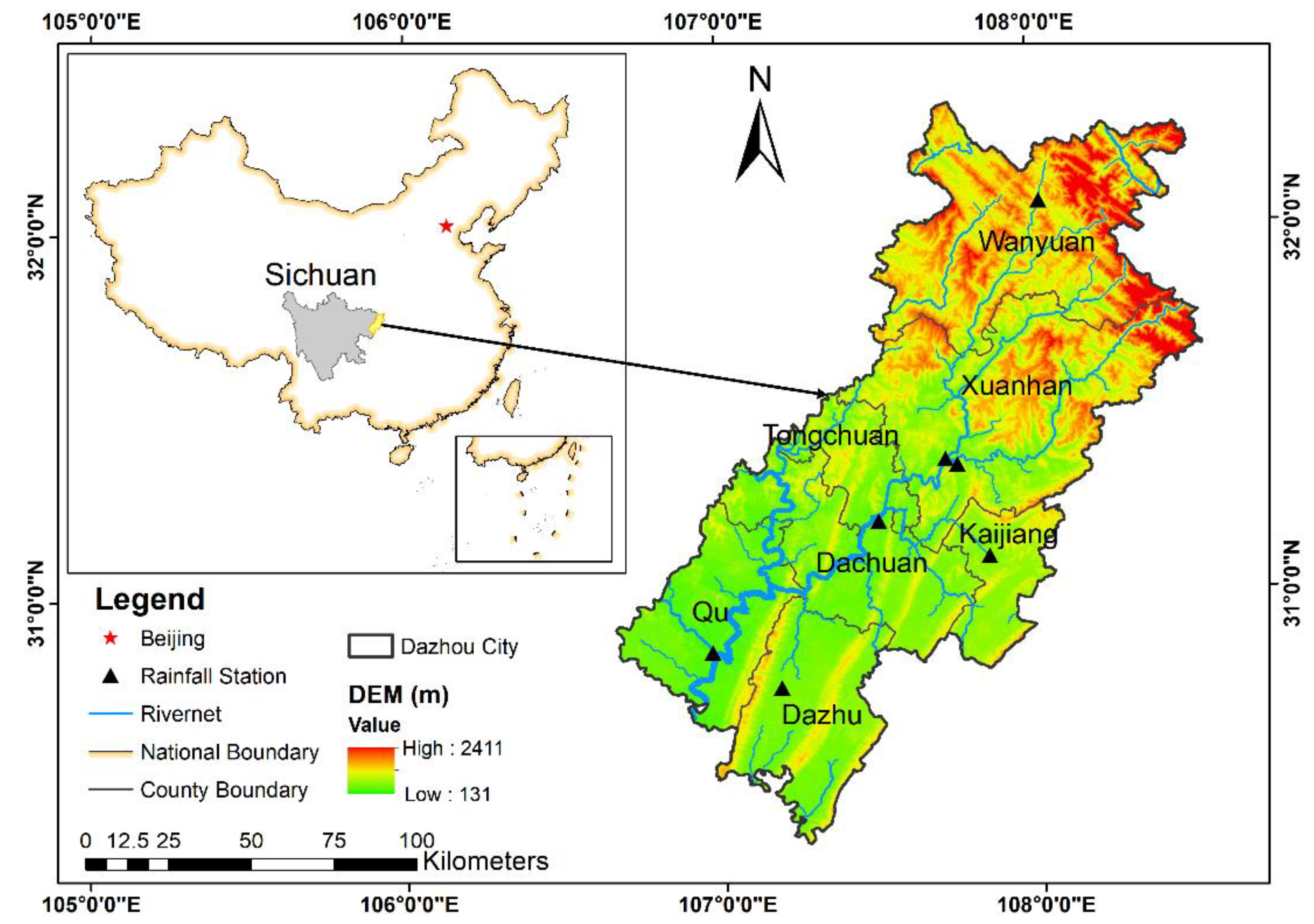
Figure 1. The location, DEM, rainfall station, and river net of the study area.
Remotesensing 14 04843 g001
Figure 2. Distribution of historical flood points in Dazhou City.
Remotesensing 14 04843 g002
Figure 3. Schematic diagram of flood hazard analysis system.
Remotesensing 14 04843 g003
Figure 4. Spatial distribution of the topographic and hydrological flood hazard factors. The factors are standardized in the range from 0 to 1. (a) Digital Elevation Model (DEM); (b) Elevation Standard Deviation (ESD); (c) Depression Point Density (DPD); (d) Flow Accumulation (FA); (e) Soil Permeability (SP); (f) Land Use (LU); (g) Distance to River (DR); and (h) Topographic Wetness Index (TWI).
Remotesensing 14 04843 g004
Figure 5. Fusion data accuracy analysis of four methods.
Remotesensing 14 04843 g005
Figure 6. Spatial distribution of maximum precipitation (MAP) factor with four durations using the LR method. (a) MAP-3 h; (b) MAP-6 h; (c) MAP-9 h; (d) MAP-12 h.
Remotesensing 14 04843 g006
Figure 7. Weights of each flood hazard factor, as listed in Table 1.
Remotesensing 14 04843 g007
Figure 8. Flood hazard distribution map in Dazhou City under four rainfall durations. (a) MAP-3 h; (b) MAP-6 h; (c) MAP-9 h; (d) MAP-12 h.
Remotesensing 14 04843 g008
Figure 9. Number of historical flood points in each hazard zone under four rainfall durations.
Remotesensing 14 04843 g009
Figure 10. Receiver Operating Characteristic (ROC) curves of the flood hazard for the four rainfall duration cases.
Remotesensing 14 04843 g010
Table 1. Nine flood hazard factors in this study.
Factor TypeSpecific FactorsAbbreviation
TopographicDigital Elevation ModelDEM
Elevation Standard DeviationDSD
Depression Point DensityDPD
HydrologicalFlow AccumulationFA
Soil PermeabilitySP
Land UseLU
Distance to RiverDR
Topographic Wetness IndexTWI
PrecipitatingMaximum PrecipitationMAP
Table 2. Soil permeability of various soil textures.
Soil TextureHaplic AlisolsCumulic AnthrosolsEutric CambisolsDystric CambisolsRendzic LeptosolsHaplic LuvisolsChromic LuvisolsGleyic LuvisolsEutric RegosolsCalcaric RegosolsWater Bodies
Soil texture code25486263100106108113156157198
Soil permeability (SP)4198567231011
Table 3. Runoff coefficients of various land use types.
Land Use TypesFarmlandForestGrasslandShrublandWetlandWaterArtificial LandNudationSparse Vegetation
Runoff coefficients0.60.150.20.180.510.950.70.9
Publisher’s Note: MDPI stays neutral with regard to jurisdictional claims in published maps and institutional affiliations.