Article

A Research on Cross-Regional Debris Flow Susceptibility Mapping Based on Transfer Learning

College of Construction Engineering, Jilin University, Changchun 130012, China
*
Author to whom correspondence should be addressed.
Remote Sens. 2022, 14(19), 4829; https://doi.org/10.3390/rs14194829
Submission received: 9 August 2022 / Revised: 14 September 2022 / Accepted: 24 September 2022 / Published: 27 September 2022

Abstract

:
Debris flow susceptibility mapping (DFSM), which has proven to be one of the most effective tools for risk management, faces a variety of problems. To realize the rational use of debris flow sample resources and improve the modeling efficiency, a unified model based on transfer learning was established for cross-regional DFSM. First, samples with 10 features collected from two debris flow-prone areas were separately used to perform factor prediction ability analysis (FPAA) based on the information gain ratio (IGR) method and then develop traditional machine learning models based on random forests (RF). Secondly, two feature matrices representing different areas were projected into a common latent feature space to obtain two new feature matrices. Then, the samples with new features were used together for FPAA and developing a unified machine learning model. Finally, the performance of the models was obtained and compared based on the area under curves (AUC) and some statistical results. All the conditioning factors played different roles in debris flow prediction in the two study areas, based on which two traditional models and a unified model were established. The unified model based on feature transferring realized efficient cross-regional modeling, solved the unconvincing problem of limited sample modeling, and enabled more accurate identification of some debris flow samples.

Graphical Abstract

1. Introduction

As the demand for deep development of surface space grows, human engineering activities in mountainous regions make the prevention and control of geological hazards increasingly become a hot topic [1]. Debris flow, with the characteristics of sudden and ferocious eruption and wide-ranging impact, is one of the major geological hazards causing the loss of human life and property. For example, a single huge debris flow that occurred in Zhouqu County, Gansu Province, China, caused up to 1765 deaths [2]. With the increasingly frequent extreme rainfall in recent years, how to deal with debris flow is an issue that deserves more attention. To minimize the possible damage caused by debris flow, the most common measures currently include monitoring, construction of protective facilities, susceptibility mapping, and so on [3]. Recently, the development of geographic information technology makes susceptibility mapping more popular in the field of debris flow risk management [4].
The methods for debris flow susceptibility mapping (DFSM) have a development trend from qualitative to quantitative [5]. Research on qualitative-based methods has been rarely conducted recently due to its high reliance on expert experience [6]. Conversely, the quantitative methods have dominated the current research by extracting related information from objective data to perform DFSM. Common quantitative models can be subdivided into four groups including physical, opinion-driven, statistical, and machine learning depending on how the data is used [7,8,9,10]. These data-driven approaches can be summarized in two steps: (1) Collect the debris flow-related data; (2) select the right algorithm model. The improvement of input data quality and algorithm performance is the key to obtaining high-quality debris flow susceptibility maps [7]. The current exploration methods to improve the quality of input data include obtaining more reliable negative samples [11,12], adopting appropriate sampling strategies [13], and adopting appropriate spatial resolution [7], etc. The comparative study of algorithms has always been one of the hotspots in DFSM [14,15]. Recently popular algorithms mainly include artificial neural networks [16], support vector machines [17], decision trees [18], random forests (RF) [19], and some other ensemble models for higher accuracy [20].
In general, after optimizing the input data and the algorithms, some models that perform well for a specific study area can always be obtained. However, some limitations are also obvious: (1) When these models are faced with a new study area, their performance is difficult to guarantee; (2) Samples within a single study area are not always sufficient to build a satisfactory model. (3) Modeling each study area separately is actually quite expensive when faced with multiple study areas.
Transfer learning, which focuses on using knowledge learned from known domains to improve models applicable to new domains, is an effective machine learning method for solving the problems mentioned above [21]. Common forms of knowledge that can be transferred include instances, features, parameters, and relationships [22]. All these approaches typically assume a sample-rich source domain and a target domain lack of samples, the purpose of transfer learning is to efficiently and reasonably transfer knowledge from the source domain to the target domain. For instance-based transfer learning, samples in the source domain are usually given different weights to assist in the establishment of a model suitable for the target domain [23]. For parameter-based transfer learning, it is often associated with deep learning algorithms. The establishment of the model follows two steps: (1) Establish a pre-trained deep learning model based on samples from the source domain. (2) Retain the parameters learned from the source domain and adjust the remaining parameters of the model based on the samples of the target domain [24]. It can be seen that both methods will make the established model more biased towards the target domain. As for relationship-based transfer learning, it is mainly used to transfer the connection between data from the source domain to the target domain. In this study, we focused on feature-based transfer learning. By projecting feature matrices representing different study areas into a common latent feature space, samples from different study areas could be used together to build a unified model.
This study is to establish a unified cross-regional DFSM model. A feature-based transfer learning method was used to reduce the feature differences between different study areas. The predictive ability of the conditioning factors obtained based on the information gain ratio (IGR) method, and the performance of the models obtained based on some related indexes was compared and discussed before and after the transferring process. This study could provide a useful reference for the efficient modeling of multi-region debris flow susceptibility mapping.

2. Materials

2.1. Study Areas and Debris Flow Inventories

Beichuan County, located in Sichuan province (Figure 1), was selected as the first study area due to the frequent debris flow events within its boundaries. It is bounded by longitudes of 103°33′E and 104°42′E and latitudes of 31°14′N and 32°14′N. It covers an area of 3084 km2 with a mountainous subtropical humid monsoon climate, which brings abundant rainfall from July to September every year. Affected by tectogenesis and long-term erosion of rivers, deep gullies, narrow valleys, and steep ridge slopes are widely distributed in Beichuan County. In terms of lithology, phyllite dominates the entire study area. Besides, mudstone, sandstone, and carbonate rocks also exist. In addition, the Longmenshan fault structure that runs through Beichuan County from the northeast to the southwest has caused extensive bedrock exposure, rock fragmentation, and soil loss, which increases the risk of debris flow. Besides, the population of up to 238,600 in Beichuan County is a high-risk threat object on the one hand, and, on the other hand, vigorous engineering activities are also an important control factor for the formation of debris flow.
Not far from Beichuan County, the Yanzi River Basin (Figure 1) in Gansu Province was chosen as the second study area. It covers an area of approximately 1276 km2 between longitudes 105°15′E–106°00′E and latitudes 32°50′N–33°25′N. Located in the transition zone from the subtropical zone to the warm temperate zone, the annual average rainfall in the Yanzi River Basin reaches 777.5 mm. Active tectonic movements and extensive river erosion make the landform types in the area mainly mountains and river valleys. As for lithology, metamorphic rocks, especially metamorphic phyllites, dominate the entire area. Besides, the accelerated construction activities in the area recently are playing an increasingly important role in debris flow formation. In general, the situation in Yanzi River Basin is quite similar to that in Beichuan County.
On the one hand, abundant rainfall, active tectonic movements, and vigorous human activities make Beichuan County and the Yanzi River Basin prone to debris flow. On the other hand, these similar characteristics also make the two study areas more suitable for transfer learning.
A reliable debris flow inventory helps build a higher quality debris flow susceptibility map [25]. The debris flows inventory for Beichuan County and the Yanzi River Basin were obtained from previous surveys and interpretations of Google Earth imagery [26,27]. Finally, 148 debris flow locations in Beichuan County and 44 debris flow locations in Yanzi River Basin were prepared for follow-up studies (Figure 1).

2.2. Data Preparation

2.2.1. Mapping Units

Appropriate mapping unit types have been proven to be helpful to improve the quality of DFSM [28]. Watershed units and grid cells are two types of the most popular mapping unit for debris flow, and each has its own advantages and disadvantages [29]. Grid cells are not directly related to debris flow and are usually more suitable for describing the local characteristics of debris flow events in applications. On the other hand, for a debris flow susceptibility map based on grid cells, multiple grid cells with different susceptibility levels might exist in a single debris flow watershed, which increases the difficulty of using the susceptibility map. The watershed unit, as the basic unit of the formation and development of debris flow, can more conveniently describe the overall characteristics of some debris flow events, such as the height difference of the watershed and the vegetation coverage in the watershed. In addition, the use of watershed units ensures the uniformity of information within a single debris flow basin, which makes it easier to identify the specific impact area of any debris flow event on the debris flow susceptibility maps [30]. In this paper, the watershed units were therefore adopted due to their ability to carry more physically meaningful topographic information and better distinguish the location of debris flow. The hydrological analysis tools of the ArcGIS platform were responsible for the division of the watershed units, a 30-m resolution digital elevation model (DEM) m from the Geospatial Data Cloud (http://www.gscloud.cn, accessed on 7 May 2022) was used as the input data and some boundaries were then manually adjusted according to Google Image.

2.2.2. Conditioning Factors

Since debris flow is the result of multiple internal and external factors, the combination of debris flow conditioning factors can be varied [31]. Considering the availability, reliability, and transferability of factors, a total of 10 conditioning factors were prepared.
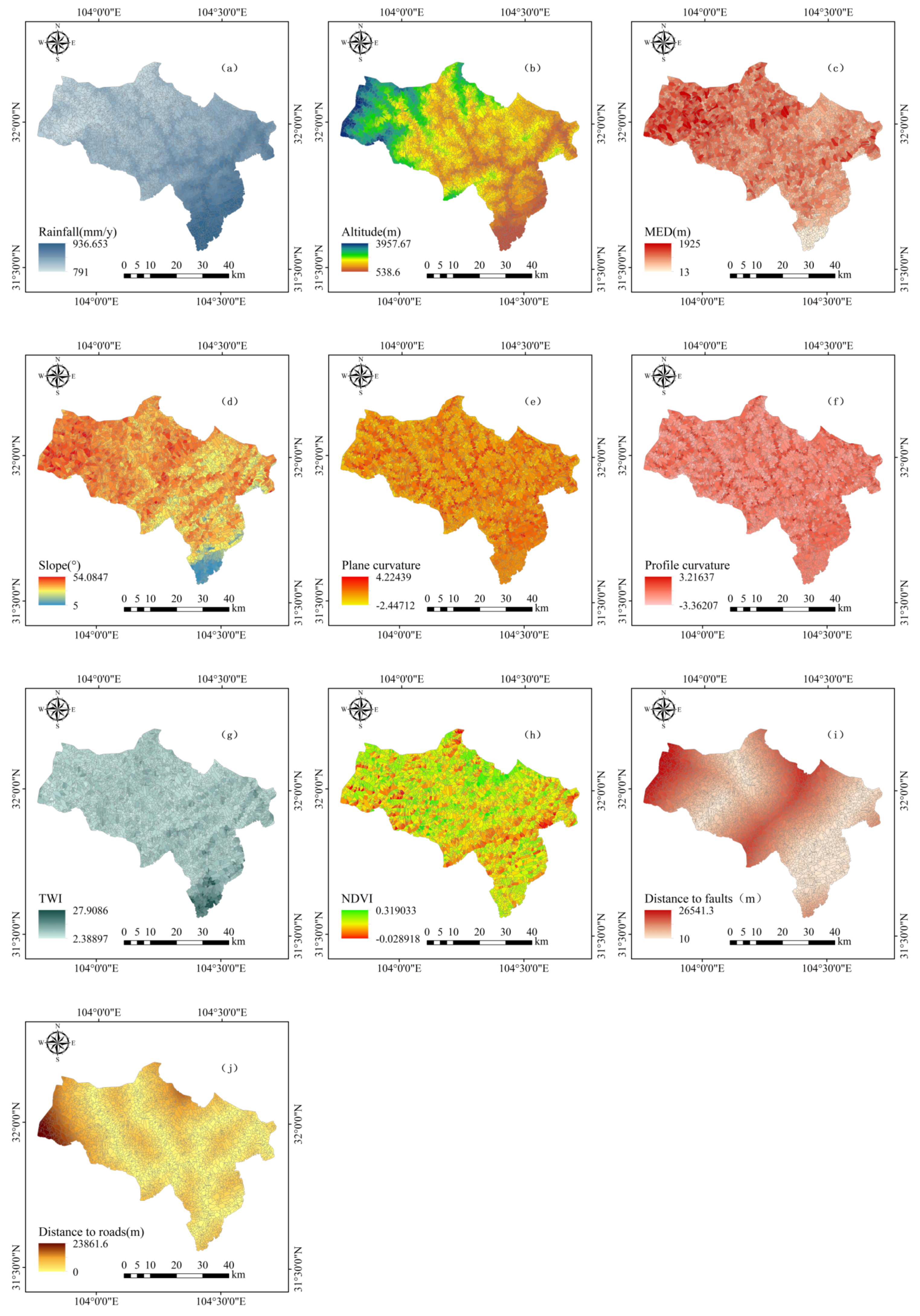
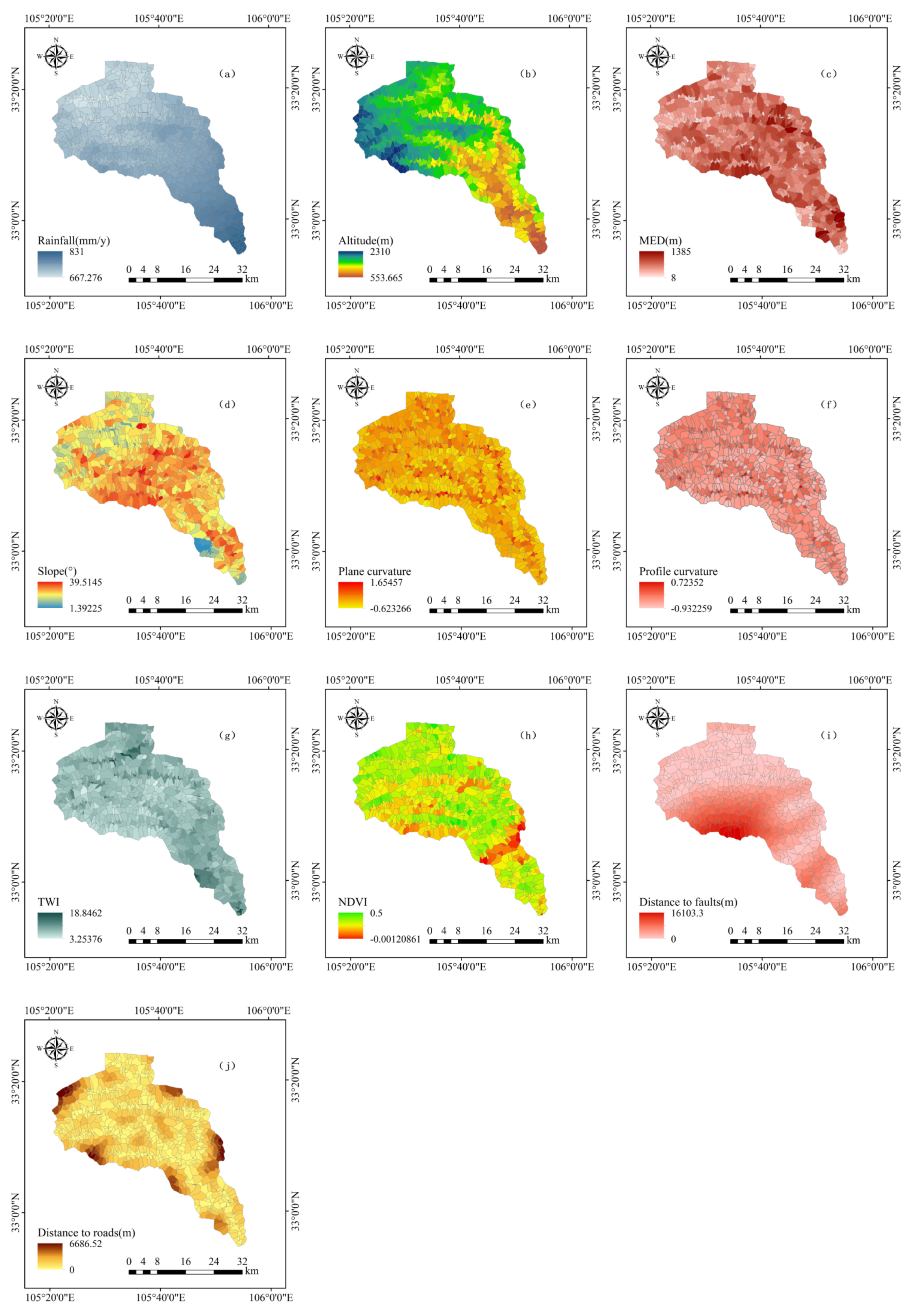
Rainfall (Figure 2a and Figure 3a) is a recognized triggering factor that controls the generation of debris flow [32,33]. The average annual rainfall (1970–2000) was therefore collected as a conditioning factor. The rainfall data comes from a climate website (worldclim.org, accessed on 7 May 2022).
Topographic factors have been widely used for DFSM [34]. Six topographic-related factors including altitude, maximum elevation difference (MED), slope, plane curvature, profile curvature, and topographic wetness index (TWI) were prepared in this paper. All these factors were generated based on the same DEM used to divide watershed units. Altitude (Figure 2b and Figure 3b) is an important factor indirectly related to the formation of debris flow, factors such as vegetation type, air temperature, rainfall, and solar radiation will show a certain degree of vertical distribution difference with the change of altitude, which makes it a popular factor in many studies of DFSM [35]. MED (Figure 2c and Figure 3c) is an important indicator reflecting the potential energy of debris flow [36]. Slope (Figure 2d and Figure 3d) is an important factor to determine the movement process of debris flow. On the other hand, since steep slopes have greater potential for instability [37,38,39,40], collapses and landslides nurtured by steep slopes could also bring potential sources for debris flow [41]. Plane curvature and profile curvature (Figure 2e,f and Figure 3e,f) are two other important parameters that determine the change of direction and velocity of debris flow [42]. TWI (Figure 2g and Figure 3g) is a physical indicator that can quantify the control effect of topography on the flow process of debris flow [43].
Surface vegetation conditions were considered in many debris flow-related studies [44]. Exposed soil and bedrock in less vegetated areas are more likely to destabilize, providing provenance for debris flow formation. In this paper, the normalized difference vegetation index (NDVI) was selected to describe the coverage of vegetation (Figure 2h and Figure 3h). The range of NDVI values is (−1, 1), where negative values indicate that visible light is highly reflected and possible surface conditions are wet bare ground, water, or snow cover. As for 0 and the positive values, the larger the value, the higher the vegetation coverage. It can be seen that in addition to directly reflecting the vegetation coverage, NDVI can also distinguish the surface conditions of areas without vegetation coverage.
In order to consider the influence of tectonic movement and human engineering activities, we used the spatial analysis tool in ArcGIS to obtain two factors: distance to faults (DTF) and distance to roads (DTR) (Figure 2i,j and Figure 3i,j). The faults were recognized from a geological map on a scale of 1:50,000. And the relevant road information was obtained based on Google Image interpretation. Generally speaking, rock formations near faults are generally more fragmented, and fractured rock formations have a greater chance of becoming a source of debris flow [45,46]. Road construction will destabilize the slope and the generated construction waste is another important source of debris flow [47,48,49].

3. Methodology

3.1. Sampling and Partitioning Strategy

As a typical binary classification problem, debris flow susceptibility mapping usually requires a relatively balanced positive and negative sample ratio to ensure that the model will not be biased towards a certain classification result [50]. However, only positive samples and a large number of unlabeled samples were available. According to previous studies [34,51], the vast majority of the two study areas are stable and debris flow is not prone to occur. Therefore, while randomly selecting negative samples among unlabeled samples might introduce some noise, most randomly selected samples can be considered reliable negative samples that are helpful for modeling. For the traditional machine learning modeling process, since 148 debris flow samples from Beichuan County and 44 debris flow samples from the Yanzi River Basin were collected, the same number of non-debris flow samples were randomly selected from the corresponding study areas, respectively. After the transferring process, we treated 192 debris flow samples from the two study areas as a whole, and 194 non-debris flow samples were randomly generated from the two study areas. With reference to previous literature [52], the datasets were all divided into two groups: 70% for the model training, and 30% for validation.

3.2. IGR

The information gain ratio (IGR) is one of the most widely used methods for factor prediction ability analysis [53]. In this paper, it not only helps us have a prior understanding of the conditioning factors before modeling but also makes it easier for us to understand the impact of transfer learning on conditioning factors. By calculating the reduction in the information entropy of the dataset conditioned on a certain factor, the importance of the conditioning factor could be quantified. In addition, the IGR method also introduces a penalty coefficient to limit the impact of factor grouping. The penalty coefficient is a parameter related to the number of conditional factor groupings, which can effectively avoid biasing factors with more groupings. The formulas are as follows:
GainRatio S , A = Gain S , A / IV A
Gain S , A = Ent S v = 1 V S v S Ent S v
IV A = v = 1 V S v S log 2 S v S
where Gain(S,A) represents the information gain of factor A; Ent(S) is the overall entropy of the dataset; IV(A) is the penalty coefficient; V is the number of attribute values; S is the entire dataset.

3.3. The Transfer Component Analysis

The transfer component analysis (TCA) method was proven to be effective in reducing the difference between the distributions of the feature matrices of two study areas, and its computational cost is generally acceptable [54]. The specific steps are as follows:
(a) The feature matrices of the two study areas were defined as Xs and Xt, respectively.
(b) A feature mapping function ϕ was introduced to project Xs and Xt into a common latent feature space.
(c) In order to solve this feature mapping function ϕ, TCA measures the distance between Xs and Xt by the maximum mean discrepancy.
dist X s , X t = 1 n 1 i = 1 n 1 ϕ x si 1 n 2 j = 1 n 1 ϕ x tj H  
where n1 and n2 are the number of samples in Xs and Xt; xsi ∈ Xs, xtj ∈ Xt; H is the Reproducing Kernel Hilbert Space.
(d) After squaring and expanding the above distance, a kernel matrix method was introduced, and the distance between Xs and Xt can be expressed as follows:
dist X s , X t = tr KL
K = K s , s K s , t K t , s K t , t R n 1 + n 2 × n 1 + n 2
K ( x i , x j ) = ϕ ( x i ) T ϕ ( x j )
L i , j = 1 n 1 2 ,     x i , x j X s 1 n 2 2 ,       x i , x j X t 1 n 1 n 2 ,   otherwise
where Ks,s, Kt,t, Ks,t and Kt,s respectively are the kernel matrix on the data in Xs and Xt and cross domains; L(i,j) is the metric matrix.
(a) To make the results more computable, a dimensionality reduction method was introduced:
dist X s , X t = tr K 0 L
K 0 = KWW T K
W = K 1 / 2 W 0 R n 1 + n 2 × m ,     m < n 1 + n 2
where K0 is the kernel matrix after dimension reduction; W0 is a low-dimensional matrix to transform the original kernel matrix.
(b) In minimizing criterion (9), considering the computational cost and preserving the data features of Xs and Xt, the final optimization objective is as follows:
min W = tr W T KLKW + μ tr W T W s . t .   W T KHKW = I m
H = I n 1 + n 2 1 n 1 + n 2 11 T
where μ is a trade-off parameter; tr(WTW) is a regularization term to control the complexity of W; Im is an identity matrix to control the divergence of the data.

3.4. RF

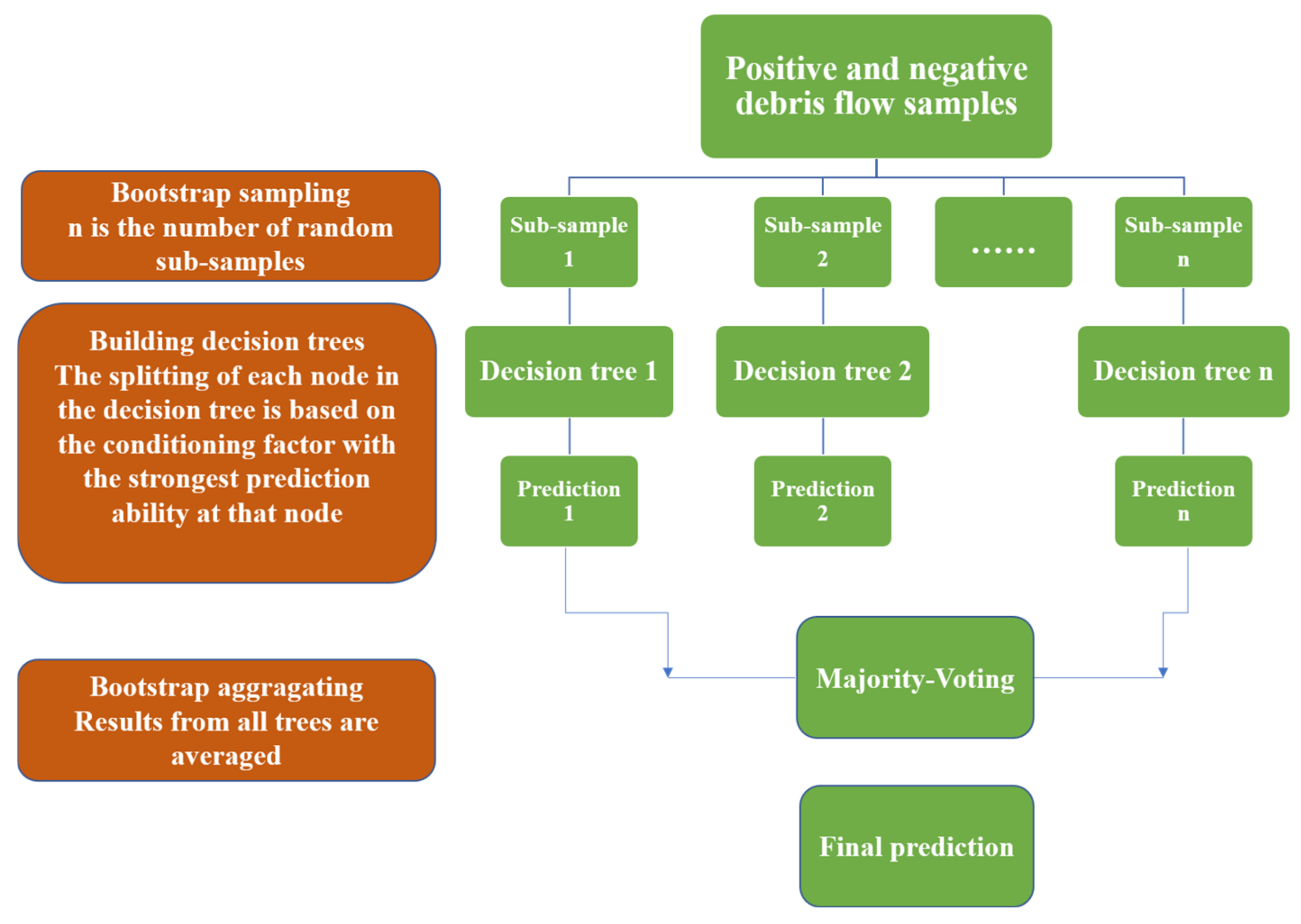
RF is one of the most popular ensemble models [19]. The specific modeling process was shown in Figure 4. It can be seen that: (1) Each decision tree was built based on a randomly generated sub-sample set. (2) Each split of the decision tree was the best split based on randomly selected features. The randomness in RF has been proved to effectively reduce the overfitting problem [55].

3.5. Receiver Operating Characteristic Curve

The receiver operating characteristic curves (ROC) has been widely used for performance evaluation of classification models in recent years [56]. It is simple and intuitive, and the areas under curves (AUC) can provide a comprehensive and reliable assessment of a model. To get the ROC curves, the predicted results of the samples need to be counted. Then we will get two metrics: sensitivity and specificity. The formulas are as follows:
Sensitivity = TP TP + FN
Specificity = TN FP + TN
where TP represents the number of correctly classified positive samples; FP represents the number of misclassified positive samples; TN represents the number of correctly classified negative samples; FN represents the number of misclassified negative samples. In the actual application process, the determination of positive samples and negative samples also needs to determine a probability threshold. With different thresholds, the final statistical results will also vary. The ROC curve takes 1-specificity as the abscissa and sensitivity as the ordinate and selects different thresholds to obtain multiple coordinate points for the curve. We plotted the ROC curve with different thresholds between 0 and 1 at 0.1 intervals. The meaning of AUC is the probability that a classifier will give a positive sample a greater score than a negative sample [57]. In previous studies, the AUC was categorized as poor (0.5–0.6), average (0.6–0.7), good (0.7–0.8), very good (0.8–0.9), and excellent (0.9–1) [58].
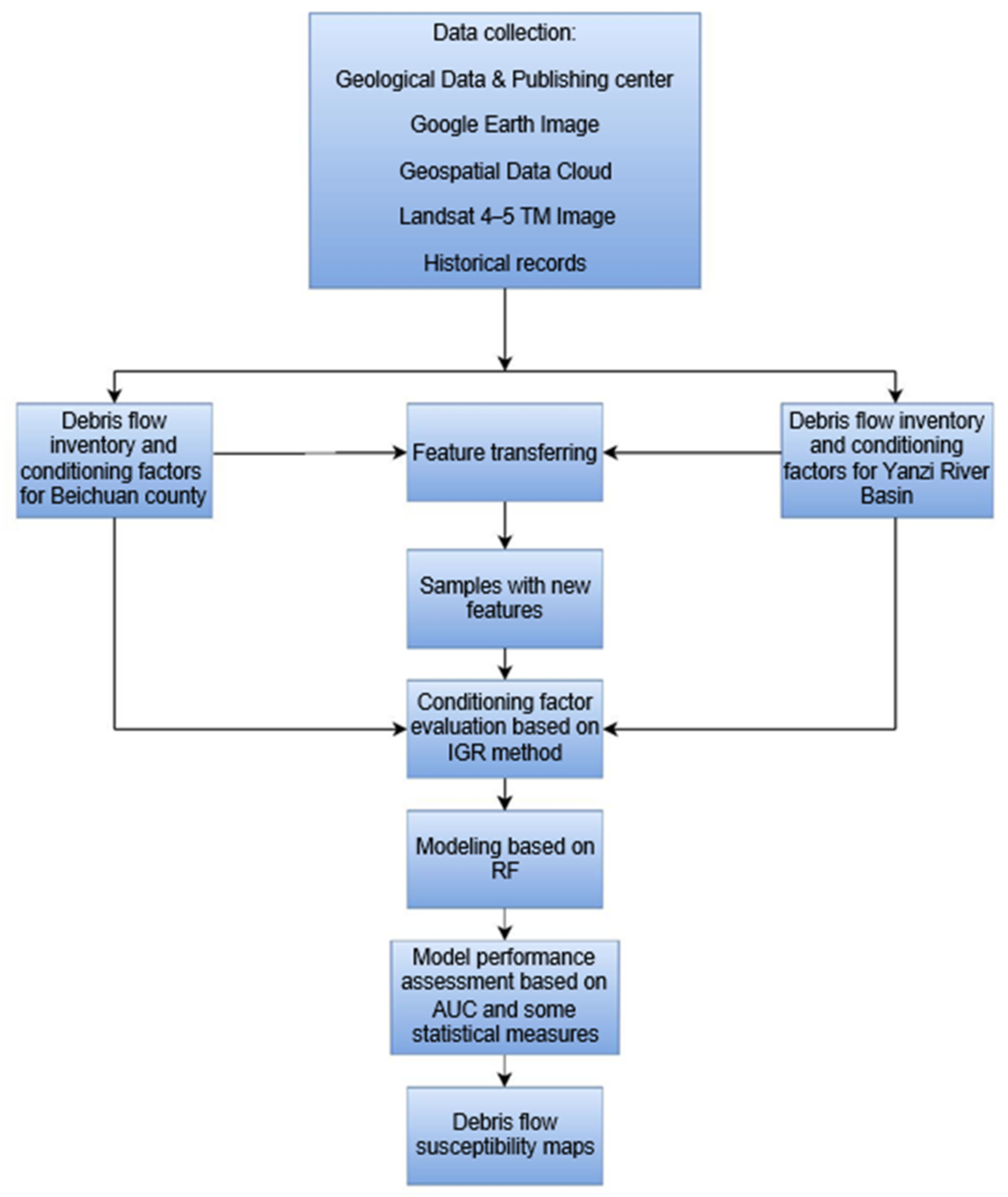
All the methodology used in this study was shown in Figure 5, which is also a flow chart of this study.

4. Results

4.1. Predictive Ability of Conditioning Factors

After feature transferring, a unified dataset with eight new conditioning factors was obtained since the dimensionality reduction method was adopted in the calculation process. The IGR values of the conditioning factors directly collected from the two study areas and the conditioning factors obtained after feature transferring were shown in Table 1. For the conditioning factors collected from the study areas, the same conditioning factor generally showed obvious differences in the predictive ability for the two study areas. At the same time, the conditioning factors with the largest IGR values in the two study areas also have some overlap as rainfall, altitude, DTF, and DTR played an important role in both study areas. For the conditioning factors obtained after transferring, the overall dispersion of IGR values is smaller, and there is also a lack of conditioning factors with strong predictive ability.

4.2. Model Performance

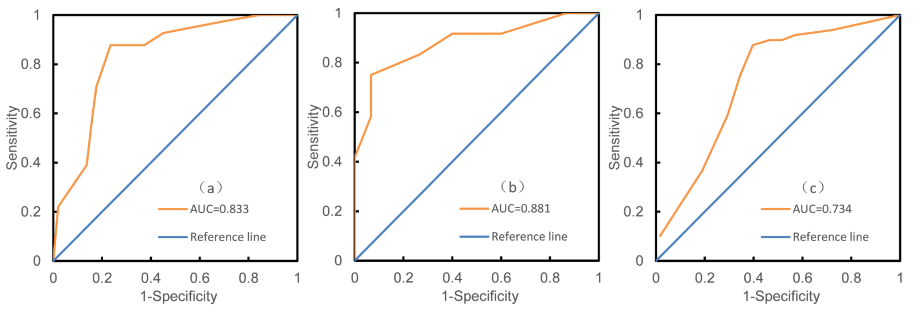
The AUC values were used to evaluate the traditional and unified models for the two study areas. For the training process (Figure 6), with the AUC value reaching 0.962, the model for Yanzi River Basin achieved the best performance, followed by the model for Beichaun County (AUC = 0.915), and the unified model performed the worst (AUC = 0.858). As for the validation process (Figure 7), the model performance ranking is still Yanzi River Basin, Beichuan County, and the unified model with the AUC values of 0.881, 0.833, and 0.734 respectively. Besides, the performance of the unified model in the validation process had dropped significantly compared to the training process, indicating a weaker generalization ability.

4.3. Rationality Analysis of Debris Flow Susceptibility Maps

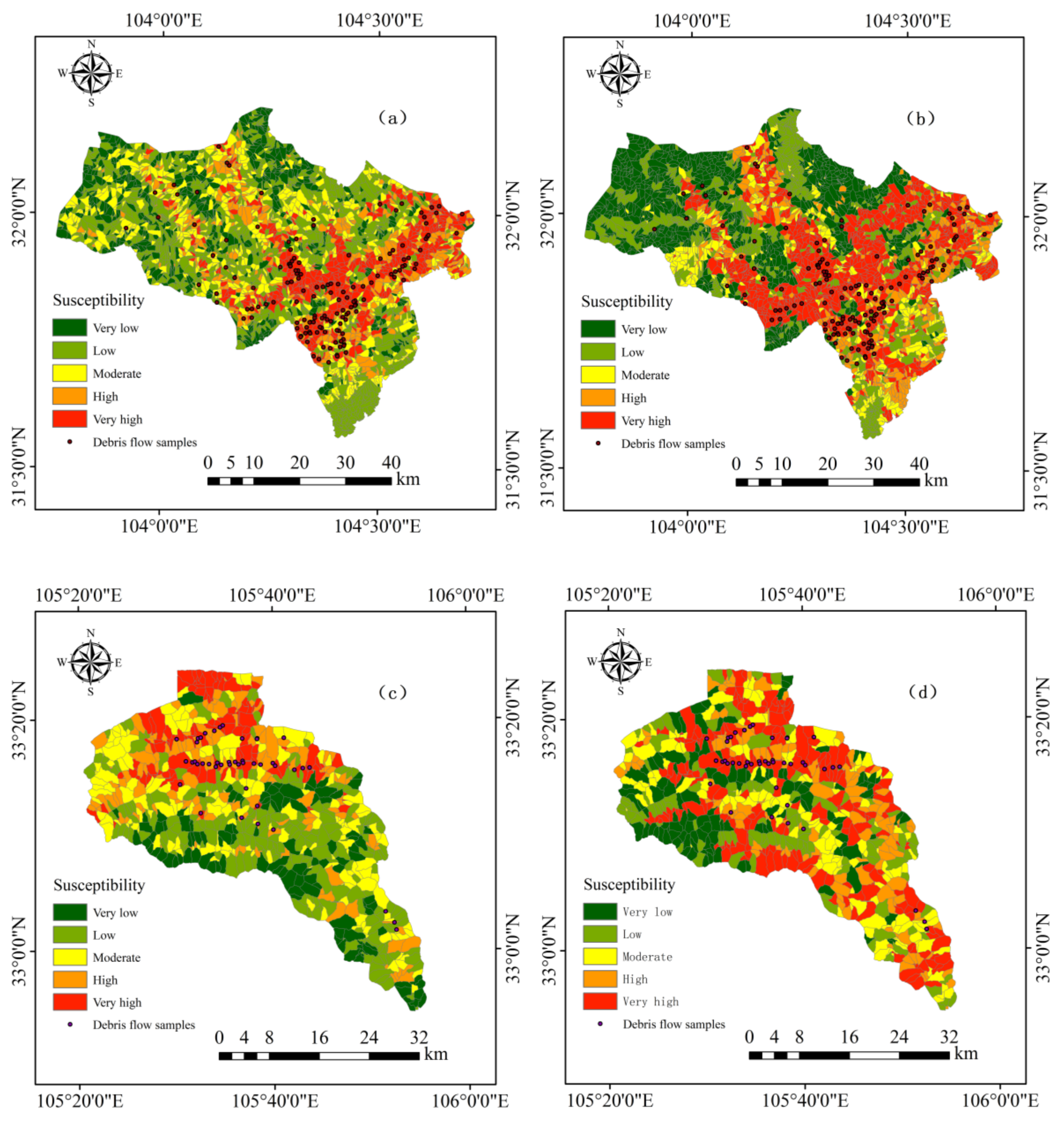
Based on two traditional models and one unified model, two susceptibility maps were obtained for each of the two study areas (Figure 8). All the susceptibility classes of the susceptibility maps were divided based on the natural break method. Statistical analysis of the predicted results of known debris flow samples is an effective method to test the rationality of the susceptibility map. Table 2 showed that the rationality of the debris flow susceptibility maps was satisfactory since most of the debris flow samples were correctly classified as having a susceptibility above moderate. In addition, the debris flow susceptibility map generated based on the unified model classified more debris flow samples as very high susceptibility but also misclassified more debris flow samples as below moderate susceptibility.

5. Discussion

5.1. Conditioning Factor Analysis

The evaluation of condition factors is an indispensable step in DFSM [7]. In previous studies, the evaluation of conditioning factors can not only help to choose appropriate factors to build more satisfactory machine learning models but also provide a better understanding of the formation of debris flow since conditioning factors with strong predictive ability are usually closely related to the formation of debris flow [59]. According to the result that conditioning factors including rainfall, altitude, DTF, and DTR made a great contribution to the prediction of debris flow in both study areas, a similar formation mechanism of debris flow in the two study areas can be inferred: (1) The high and steep mountainous landforms provide favorable topographical conditions for the formation of debris flow. (2) The fractured rock and soil mass near the fault and the deposits directly or indirectly caused by human engineering activities provide abundant provenance for the debris flow. (3) Rainfall is the main source of hydrodynamics for the formation of debris flows in the two study areas. The similarity is the basis for subsequent transfer learning.
After feature transferring, since each conditioning factor might be a coupling of multiple directly collected conditioning factors, the overall dispersion of IGR values became smaller. Besides, this kind of coupling may mask some information useful for debris flow prediction, which makes the conditioning factors with strong predictive power lacking in the unified dataset.

5.2. Comparison of Traditional and Unified Models

In this study, the performance of the models is a reflection of the data quality since all the models were based on the same RF algorithm. The result that the model for Yanzi River Basin performed better than the model for Beichuan County indicated the higher quality of the Yanzi River Basin dataset, which may be due to the fact that more randomly generated non-debris flow samples in Beichuan County have introduced more noise to its dataset. However, there are also some problems with the model for the Yanzi River Basin because of the small dataset. On the one hand, insufficient training samples cannot enable the model to learn the general characteristics of debris flow well. On the other hand, the generalization ability of the model tested based on insufficient validation samples is actually not convincing enough. Since labeling samples and modeling is a difficult and time-consuming process, it is necessary and meaningful to build a unified model applicable across regions that can reasonably utilize the samples from both study areas at the same time. Considering the samples in Beichuan County as the source domain and the samples in the Yanzi River Basin as the target domain, transfer learning has been proven to have the potential to address this problem well [21]. Instance-based, parameter-based and feature-based methods are the most recent commonly used approaches. The instance-based approach focused on building a model that performs well in the target domain, which requires assigning different weights to samples from the source domain to participate in the modeling as auxiliary samples [23]. For a parameter-based approach, deep learning algorithms are often employed, and samples from the source domain and the target domain played the role of pre-training and fine-tuning respectively in the modeling process [24]. Both of the final models will not only be biased towards the target domain but also have higher requirements on algorithms and samples from both the source and target domains. In this paper, the feature-based approach was finally adopted. By projecting feature matrices representing different study areas into a common latent feature space, a unified dataset was built, and then the RF algorithm was utilized to build a unified model. Obviously, the feature-based approach has lower sample requirements, more flexible algorithm selection, and more balanced consideration of source and target domains.
The final unified model in this paper still has some limitations such as not performing as well as the traditional model. Although a feature transferring method was used to reduce the difference in feature distribution between the two study areas, the difference still existed. And this kind of difference is one of the main sources of dataset noise. The union of the datasets of the two study areas also increases the noise in the unified dataset. Noise in a dataset can seriously affect the generalization ability of a model. Besides, the RF algorithm used in this paper is an ensemble learning algorithm with decision trees as weak classifiers. The split of each node of the decision tree depends on some conditioning factors with strong predictive ability [55]. The lack of conditioning factors with strong predictive ability in the unified dataset degraded the performance of the model to a certain extent. Considering the meaning of AUC, it can be seen from Figure 8 that the poor performance of the unified model is mainly reflected in the overprediction of the probability of some negative samples, which indicates that the unified model is a more conservative model. Actually, the performance of the unified model is generally acceptable with the AUC values of 0.858 for the training process and 0.734 for the validation process, especially for the cross-regional modeling.
The statistical results of the classification of known debris flow samples are important indicators for evaluating the rationality of debris flow susceptibility maps [51]. And more details of the classification of the samples can also help us understand the models more comprehensively compared to the model evaluation based on the AUC values [34]. The result that the debris flow susceptibility maps generated based on the unified model misclassified more debris flow samples as below medium susceptibility is another intuitive manifestation of the relatively poor performance of the unified model. Besides, the unified model classified more debris flow samples as very high susceptibility, that is, it enabled more accurate identification of some debris flow samples, which might be due to the removal of some redundant information by dimensionality reduction when obtaining the unified dataset. More accurate identification of debris flow samples can effectively improve the practical value of the corresponding debris flow susceptibility map.

5.3. Limitations

This paper focused on the establishment of a unified model for cross-regional DFSM. A generally satisfactory model was built, with some limitations remaining: (1) Ten conditional factors belonging to continuous variables are used in this study, and more factors that are closely related to debris flow and have strong predictive ability can be considered to provide better options. (2) The non-debris flow samples in all datasets were randomly obtained, and some more reasonable non-debris flow sample acquisition methods should be utilized to improve the model performance. (3) More noise was introduced in the process of establishing the unified dataset, some advanced data cleaning methods such as binning and clustering can be utilized to improve dataset quality. (4) Only a single RF algorithm was used in this paper, and more advanced algorithms can be discussed and compared.

6. Conclusions

DFSM has been developed for years, and most of the research has focused on dataset quality and algorithm improvements. In the present study, a unified model that can address the problem of insufficient sample size and is applicable to multiple study areas was established and compared, and the following conclusions could be drawn:
  • The same conditioning factors have different prediction abilities of debris flow in different study areas, but the similarity of debris flow control factors in different study areas is the basis for feature transferring.
  • The unified model based on feature transferring can solve the problem that it is difficult to build a convincing model with limited samples while ensuring a certain accuracy.
  • More accurate identification of some debris flow samples makes the unified model more helpful for debris flow risk management.

Author Contributions

R.G., writing—original draft, methodology and software; C.W., validation; S.H., code inspection; H.L. and X.L., software and validation; D.W., reviewing and editing. All authors have read and agreed to the published version of the manuscript.

Funding

This research was funded by the National Natural Science Foundation of China (Grant No. 41972267).

Data Availability Statement

The data used to support the findings of this study are provided by the Geoscientific Data & Discovery Publishing System, Geospatial Data Cloud and Earth System Science Data Discussions.

Acknowledgments

The authors of this article are grateful for the National Natural Science Foundation of China (Grant No. 41972267).

Conflicts of Interest

The authors declare no conflict of interest.

References

  1. Huang, H.; Wang, Y.; Li, Y.; Zhou, Y.; Zeng, Z. Debris-Flow Susceptibility Assessment in China: A Comparison between Traditional Statistical and Machine Learning Methods. Remote Sens. 2022, 14, 4475. [Google Scholar] [CrossRef]
  2. Chong, Y.; Chen, G.; Meng, X.; Yang, Y.; Shi, W.; Bian, S.; Zhang, Y.; Yue, D. Quantitative analysis of artificial dam failure effects on debris flows–A case study of the Zhouqu ‘8.8’ debris flow in northwestern China. Sci. Total Environ. 2021, 792, 148439. [Google Scholar] [CrossRef] [PubMed]
  3. Ciurleo, M.; Mandaglio, M.C.; Moraci, N. A quantitative approach for debris flow inception and propagation analysis in the lead up to risk management. Landslides 2021, 18, 2073–2093. [Google Scholar] [CrossRef]
  4. Pham, B.T.; Bui, D.T.; Prakash, I.; Dholakia, M. Hybrid integration of Multilayer Perceptron Neural Networks and machine learning ensembles for landslide susceptibility assessment at Himalayan area (India) using GIS. Catena 2017, 149, 52–63. [Google Scholar] [CrossRef]
  5. Corominas, J.; van Westen, C.; Frattini, P.; Casini, L.; Malet, J.-P.; Fotopoulou, S.; Catani, F.; Van Den Eeckhaut, M.; Mavrouli, O.; Agliardi, F.; et al. Recommendations for the quantitative analysis of landslide risk. Bull. Eng. Geol. Environ. 2014, 73, 209–263. [Google Scholar] [CrossRef]
  6. Yao, X.; Tham, L.G.; Dai, F.C. Landslide susceptibility mapping based on support vector machine: A case study on natural slopes of Hong Kong, China. Geomorphology 2008, 101, 572–582. [Google Scholar] [CrossRef]
  7. Chang, K.T.; Merghadi, A.; Yunus, A.P.; Pham, B.T.; Dou, J. Evaluating scale effects of topographic variables in landslide susceptibility models using GIS-based machine learning techniques. Sci. Rep. 2019, 9, 12296. [Google Scholar] [CrossRef]
  8. Nguyen, M.D.; Pham, B.T.; Tuyen, T.; Yen, H.P.H.; Prakash, I.; Thanh, T.V.; Chapi, K.; Shirzadi, A.; Shahabi, H.; Dou, J.; et al. Development of an Artificial Intelligence Approach for Prediction of Consolidation Coefficient of Soft Soil: A Sensitivity Analysis. Open Constr. Build. Technol. 2019, 13, 178–188. [Google Scholar] [CrossRef]
  9. Pham, B.T.; Prakash, I.; Dou, J.; Singh, S.K.; Trinh, P.T.; Tran, H.T.; Le, T.M.; Van, P.T.; Khoi, D.K.; Shirzadi, A.; et al. A novel hybrid approach of landslide susceptibility modelling using rotation forest ensemble and different base classifiers. Geocarto Int. 2019, 35, 1267–1292. [Google Scholar] [CrossRef]
  10. Tien, B.D.; Shirzadi, A.; Shahabi, H.; Geertsema, M.; Omidvar, E.; Clague, J.J.; Thai Pham, B.; Dou, J.; Talebpour, A.D.; Bin Ahmad, B.; et al. New Ensemble Models for Shallow Landslide Susceptibility Modeling in a Semi-Arid Watershed. Forests 2019, 10, 743. [Google Scholar] [CrossRef] [Green Version]
  11. Denis, F.; Gilleron, R.; Letouzey, F. Learning from positive and unlabeled examples. Theor. Comput. Sci. 2005, 348, 70–83. [Google Scholar] [CrossRef]
  12. Liang, Z.; Wang, C.; Duan, Z.; Liu, H.; Liu, X.; Ullah Jan Khan, K. A Hybrid Model Consisting of Supervised and Unsupervised Learning for Landslide Susceptibility Mapping. Remote Sens. 2021, 13, 1464. [Google Scholar] [CrossRef]
  13. Dou, J.; Yunus, A.P.; Merghadi, A.; Shirzadi, A.; Nguyen, H.; Hussain, Y.; Avtar, R.; Chen, Y.; Pham, B.T.; Yamagishi, H. Different sampling strategies for predicting landslide susceptibilities are deemed less consequential with deep learning. Sci. Total Environ. 2020, 720, 137320. [Google Scholar] [CrossRef] [PubMed]
  14. Hong, H.; Pourghasemi, H.R.; Pourtaghi, Z.S. Landslide susceptibility assessment in Lianhua County (China): A comparison between a random forest data mining technique and bivariate and multivariate statistical models. Geomorphology 2016, 259, 105–118. [Google Scholar] [CrossRef]
  15. Huang, F.; Cao, Z.; Guo, J.; Jiang, S.-H.; Li, S.; Guo, Z. Comparisons of heuristic, general statistical and machine learning models for landslide susceptibility prediction and mapping. Catena 2020, 191, 104580. [Google Scholar] [CrossRef]
  16. Tunusluoglu, M.C.; Gokceoglu, C.; Sonmez, H.; Nefeslioglu, H.A. An artificial neural network application to produce debris source areas of Barla, Besparmak, and Kapi Mountains (NW Taurids, Turkey). Nat. Hazards Earth Syst. Sci. 2007, 7, 557–570. [Google Scholar] [CrossRef]
  17. Hong, H.; Pradhan, B.; Jebur, M.N.; Bui, D.T.; Xu, C.; Akgun, A. Spatial prediction of landslide hazard at the Luxi area (China) using support vector machines. Environ. Earth Sci. 2016, 75, 40. [Google Scholar] [CrossRef]
  18. Chen, W.; Xie, X.; Peng, J.; Wang, J.; Duan, Z.; Hong, H. GIS-based landslide susceptibility modelling: A comparative assessment of kernel logistic regression, Naive-Bayes tree, and alternating decision tree models. Geomat. Nat. Hazards Risk 2017, 8, 950–973. [Google Scholar] [CrossRef]
  19. Trigila, A.; Iadanza, C.; Esposito, C.; Scarascia-Mugnozza, G. Comparison of Logistic Regression and Random Forests techniques for shallow landslide susceptibility assessment in Giampilieri (NE Sicily, Italy). Geomorphology 2015, 249, 119–136. [Google Scholar] [CrossRef]
  20. Pham, B.T.; Nguyen-Thoi, T.; Qi, C.C.; Phong, T.V.; Dou, J.; Lanh, S.H.; Hiep, V.L.; Prakash, I. Coupling RBF neural network with ensemble learning techniques for landslide susceptibility mapping. Catena 2020, 195, 104805. [Google Scholar] [CrossRef]
  21. Zhuang, F.; Qi, Z.; Duan, K.; Xi, D.; Zhu, Y.; Zhu, H.; Xiong, H.; He, Q. A Comprehensive Survey on Transfer Learning. Proc. IEEE 2021, 109, 43–76. [Google Scholar] [CrossRef]
  22. Pan, S.J.; Yang, Q. A Survey on Transfer Learning. IEEE Trans. Knowl. Data Eng. 2010, 22, 1345–1359. [Google Scholar] [CrossRef]
  23. Dai, W.; Qiang, Y.; Xue, G. Boosting for transfer learning. In Proceedings of the Twenty-Fourth International Conference on Machine Learning (ICML 2007), Corvallis, OR, USA, 20–24 June 2007. [Google Scholar]
  24. Zhao, G.; Pang, B.; Xu, Z.; Cui, L.; Wang, J.; Zuo, D.; Peng, D. Improving urban flood susceptibility mapping using transfer learning. J. Hydrol. 2021, 602, 126777. [Google Scholar] [CrossRef]
  25. Xiong, K.; Adhikari, B.R.; Stamatopoulos, C.A.; Zhan, Y.; Wu, S.; Dong, Z.; Di, B. Comparison of Different Machine Learning Methods for Debris Flow Susceptibility Mapping: A Case Study in the Sichuan Province, China. Remote Sens. 2020, 12, 295. [Google Scholar] [CrossRef]
  26. Fan, X.; Scaringi, G.; Domènech, G.; Yang, F.; Guo, X.; Dai, L.; He, C.; Xu, Q.; Huang, R. Two multi-temporal datasets to track the enhanced landsliding after the 2008 Wenchuan earthquake. Earth Syst. Sci. Data 2019, 11, 35–55. [Google Scholar] [CrossRef]
  27. Yang, Q.; Wang, S.Y.; Ye, Z.N. Analysis on the development of geological hazard and failure mode in Yanzi River Basin. J. Eng. Geol. 2019, 27, 289–295. [Google Scholar]
  28. Guzzetti, F.; Reichenbach, P.; Ardizzone, F.; Cardinali, M.; Galli, M. Estimating the quality of landslide susceptibility models. Geomorphology 2006, 81, 166–184. [Google Scholar] [CrossRef]
  29. Zêzere, J.; Pereira, S.; Melo, R.; Oliveira, S.; Garcia, R. Mapping landslide susceptibility using data-driven methods. Sci. Total Environ. 2017, 589, 250–267. [Google Scholar] [CrossRef]
  30. Qin, S.; Lv, J.; Cao, C.; Ma, Z.; Hu, X.; Liu, F.; Qiao, S.; Dou, Q. Mapping debris flow susceptibility based on watershed unit and grid cell unit: A comparison study. Geomat. Nat. Hazards Risk 2018, 10, 1648–1666. [Google Scholar] [CrossRef]
  31. Reichenbach, P.; Rossi, M.; Malamud, B.; Mihir, M.; Guzzetti, F. A review of statistically-based landslide susceptibility models. Earth Sci. Rev. 2018, 180, 60–91. [Google Scholar] [CrossRef]
  32. Mondini, A.; Guzzetti, F.; Reichenbach, P.; Rossi, M.; Cardinali, M.; Ardizzone, F. Semi-automatic recognition and mapping of rainfall induced shallow landslides using optical satellite images. Remote Sens. Environ. 2011, 115, 1743–1757. [Google Scholar] [CrossRef]
  33. Dou, J.; Yunus, A.P.; Xu, Y.; Zhu, Z.; Chen, C.-W.; Sahana, M.; Khosravi, K.; Yang, Y.; Pham, B.T. Torrential rainfall-triggered shallow landslide characteristics and susceptibility assessment using ensemble data-driven models in the Dongjiang Reservoir Watershed, China. Nat. Hazards 2019, 97, 579–609. [Google Scholar] [CrossRef]
  34. Gao, R.; Wang, C.; Liang, Z.; Han, S.; Li, B. A Research on Susceptibility Mapping of Multiple Geological Hazards in Yanzi River Basin, China. ISPRS Int. J. Geo-Inf. 2021, 10, 218. [Google Scholar] [CrossRef]
  35. Hong, H.; Pradhan, B.; Xu, C.; Bui, D.T. Spatial prediction of landslide hazard at the Yihuang area (China) using two-class kernel logistic regression, alternating decision tree and support vector machines. Catena 2015, 133, 266–281. [Google Scholar] [CrossRef]
  36. Liang, Z.; Wang, C.; Han, S.; Khan, K.U.J.; Liu, Y. Classification and susceptibility assessment of debris flow based on a semiquantitative method combination of the fuzzy C-means algorithm, factor analysis and efficacy coefficient. Nat. Hazards Earth Syst. Sci. 2020, 20, 1287–1304. [Google Scholar] [CrossRef]
  37. Zhu, C.; He, M.; Karakus, M.; Cui, X.; Tao, Z. Investigating Toppling Failure Mechanism of Anti-dip Layered Slope due to Excavation by Physical Modelling. Rock Mech. Rock Eng. 2020, 53, 5029–5050. [Google Scholar] [CrossRef]
  38. Zhu, C.; He, M.; Karakus, M.; Zhang, X.; Tao, Z. Numerical simulations of the failure process of anaclinal slope physical model and control mechanism of negative Poisson’s ratio cable. Bull. Eng. Geol. Environ. 2021, 80, 3365–3380. [Google Scholar] [CrossRef]
  39. Tao, Z.; Geng, Q.; Zhu, C.; He, M.; Cai, H.; Pang, S.; Meng, X. The mechanical mechanisms of large-scale toppling failure for counter-inclined rock slopes. J. Geophys. Eng. 2019, 16, 541–558. [Google Scholar] [CrossRef]
  40. Dong, M.; Zhang, F.; Lv, J.; Hu, M.; Li, Z. Study on deformation and failure law of soft-hard rock interbedding toppling slope base on similar test. Bull. Eng. Geol. Environ. 2020, 79, 4625–4637. [Google Scholar] [CrossRef]
  41. Varnes, D.J. Landslide Hazard Zonation: A Review of Principles and Practice; United Nations: Paris, France, 1984; p. 63. [Google Scholar]
  42. Oh, H.J.; Pradhan, B. Application of a neuro-fuzzy model to landslide-susceptibility mapping for shallow landslides in a tropical hilly area. Comput. Geosci. 2011, 37, 1264–1276. [Google Scholar] [CrossRef]
  43. Pourghasemi, H.R.; Jirandeh, A.G.; Pradhan, B.; Xu, C.; Gokceoglu, C. Landslide susceptibility mapping using support vector machine and GIS at the Golestan Province, Iran. J. Earth Syst. Sci. 2013, 122, 349–369. [Google Scholar] [CrossRef] [Green Version]
  44. Vasu, N.N.; Lee, S.-R. A hybrid feature selection algorithm integrating an extreme learning machine for landslide susceptibility modeling of Mt. Woomyeon, South Korea. Geomorphology 2016, 263, 50–70. [Google Scholar] [CrossRef]
  45. Dong, M.; Zhang, F.; Yu, C.; Lv, J.; Zhou, H.; Li, Y.; Zhong, Y. Influence of a Dominant Fault on the Deformation and Failure Mode of Anti-dip Layered Rock Slopes. KSCE J. Civ. Eng. 2022, 26, 3430–3439. [Google Scholar] [CrossRef]
  46. Zhu, C.; Xu, X.; Wang, X.; Xiong, F.; Tao, Z.; Lin, Y.; Chen, J. Experimental Investigation on Nonlinear Flow Anisotropy Behavior in Fracture Media. Geofluids 2019, 2019, 5874849. [Google Scholar] [CrossRef]
  47. Dong, M.; Zhang, F.; Lv, J.; Fei, Y.; Li, Z. Study of Stability Influencing Factors of Excavated Anti-Dip Rock Slope. KSCE J. Civ. Eng. 2020, 24, 2293–2303. [Google Scholar] [CrossRef]
  48. Dong, M.; Kulatilake, P.H.S.W.; Zhang, F. Deformation and stability investigations in 3-D of an excavated rock slope in a hydroelectric power station in China. Comput. Geotech. 2017, 96, 132–149. [Google Scholar] [CrossRef]
  49. Zhigang, T.; Chun, Z.; Manchao, H.; Kuiming, L. Research on the safe mining depth of anti-dip bedding slope in Changshanhao Mine. Geomech. Geophys. Geo-Energ. Geo-Resour. 2020, 6, 36. [Google Scholar] [CrossRef]
  50. Kornejady, A.; Ownegh, M.; Bahremand, A. Landslide susceptibility assessment using maximum entropy model with two different data sampling methods. Catena 2017, 152, 144–162. [Google Scholar] [CrossRef]
  51. Gao, R.; Wang, C.M.; Liang, Z. Comparison of different sampling strategies for debris flow susceptibility mapping: A case study using the centroids of the scarp area, flowing area and accumulation area of debris flow watersheds. J. Mt. Sci. 2021, 18, 1476–1488. [Google Scholar] [CrossRef]
  52. Merghadi, A.; Yunus, A.P.; Dou, J.; Whiteley, J.; Thai, P.B.; Bui, D.T.; Avtar, R.; Abderrahmane, B. Machine learning methods for landslide susceptibility studies: A comparative overview of algorithm performance. Earth Sci. Rev. 2020, 207, 103225. [Google Scholar] [CrossRef]
  53. Dou, J.; Yunus, A.P.; Bui, D.T.; Merghadi, A.; Sahana, M.; Zhu, Z.F.; Chen, C.W.; Han, Z.; Pham, B.T. Improved landslide assessment using support vector machine with bagging, boosting, and stacking ensemble machine learning framework in a mountainous watershed, Japan. Landslides 2020, 17, 641–658. [Google Scholar] [CrossRef]
  54. Pan, S.J.; Tsang, I.W.; Kwok, J.T.; Yang, Q. Domain Adaptation via Transfer Component Analysis. IEEE Trans. Neural Netw. 2011, 22, 199–210. [Google Scholar] [CrossRef] [PubMed]
  55. Breiman, L. Random Forests. Mach. Learn. 2001, 45, 5–32. [Google Scholar] [CrossRef]
  56. Provost, F.; Fawcett, T. Robust classification for imprecise environments. Mach. Learn. 2001, 42, 203–231. [Google Scholar] [CrossRef]
  57. Pontius, R.G.; Parmentier, B. Recommendations for using the relative operating characteristic (ROC). Landsc. Ecol. 2014, 29, 367–382. [Google Scholar] [CrossRef]
  58. Chen, W.; Pourghasemi, H.R.; Naghibi, S.A. A comparative study of landslide susceptibility maps produced using support vector machine with different kernel functions and entropy data mining models in China. Bull. Eng. Geol. Environ. 2018, 77, 647–664. [Google Scholar] [CrossRef]
  59. Dai, F.; Lee, C.; Ngai, Y. Landslide risk assessment and management: An overview. Eng. Geol. 2002, 64, 65–87. [Google Scholar] [CrossRef]
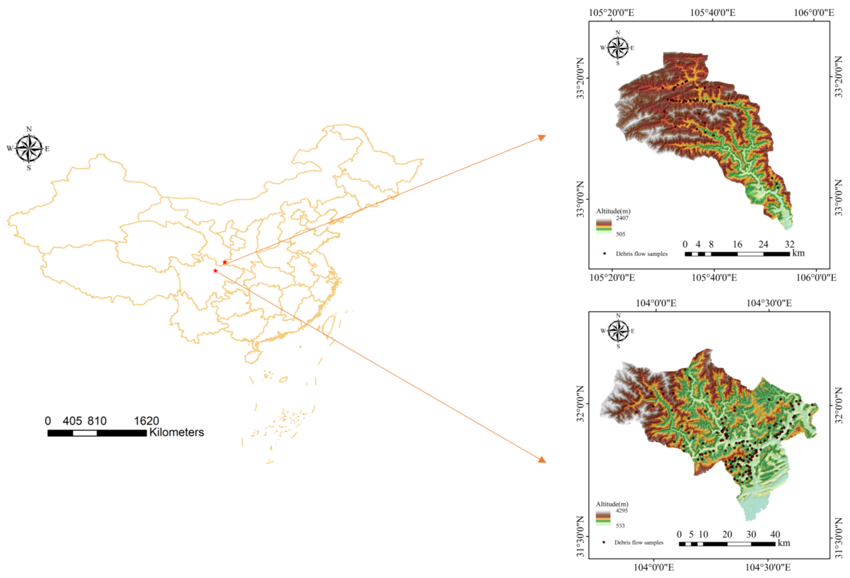
Figure 1. Location of the study areas with debris flows inventory maps.
Remotesensing 14 04829 g001
Figure 2. Conditioning factors of Beichuan County: (a) Rainfall; (b) Altitude; (c) MED; (d) Slope; (e) Plane curvature; (f) Profile curvature; (g) TWI; (h) NDVI; (i) DTF; (j) DTR.
Remotesensing 14 04829 g002
Figure 3. Conditioning factors of Yanzi River Basin: (a) Rainfall; (b) Altitude; (c) MED; (d) Slope; (e) Plane curvature; (f) Profile curvature; (g) TWI; (h) NDVI; (i) DTF; (j) DTR.
Remotesensing 14 04829 g003
Figure 4. The schematic diagram of RF.
Remotesensing 14 04829 g004
Figure 5. Flow chart of the method in this paper.
Remotesensing 14 04829 g005
Figure 6. The ROC curves based on the training dataset: (a) of the model for Beichuan County; (b) of the model for Yanzi River Basin; (c) of the unified model.
Remotesensing 14 04829 g006
Figure 7. The ROC curves based on the validation dataset: (a) of the model for Beichuan County; (b) of the model for Yanzi River Basin; (c) of the unified model.
Remotesensing 14 04829 g007
Figure 8. The debris flow susceptibility maps based on the: (a) Traditional model for Beichaun County; (b) Unified model for Beichuan County; (c) Traditional model for Yanzi River Basin; (d) Unified model for Yanzi River Basin.
Remotesensing 14 04829 g008
Table 1. The IGR values of different datasets.
DatasetConditioning FactorsIGR Values
Beichuan CountyRainfall0.097564
Altitude0.072134
DTR0.042283
NDVI0.022192
DTF0.021838
Slope0.013836
Profile curvature0.013714
TWI0.013245
MED0.009153
Plane curvature0.008380
Yanzi River BasinRainfall0.092418
DTF0.066653
Plane curvature0.059207
Altitude0.056922
DTR0.056264
MED0.026565
Slope0.021594
NDVI0.019191
TWI0.016053
Profile curvature0.014756
The unified datasetFactor 10.068698
Factor 20.028859
Factor 30.021048
Factor 40.020926
Factor 50.019072
Factor 60.019056
Factor 70.012737
Factor 80.009777
Table 2. The sample statistical results of different models.
ModelGroupsNo. of
Debris Flow Samples
Percentage of
Debris Flow Samples
Traditional model for Beichuan CountyVery low10.7%
Low85.4%
Moderate128.1%
High3725.0%
Very high9060.8%
Unified model for Beichuan CountyVery low74.7%
Low96.1%
Moderate85.4%
High2617.6%
Very high9866.2%
Traditional model for Yanzi River BasinVery low00.0%
Low12.3%
Moderate613.6%
High1431.8%
Very high2352.3%
Unified model for Yanzi River BasinVery low12.3%
Low36.8%
Moderate36.8%
High1125.0%
Very high2659.1%
Publisher’s Note: MDPI stays neutral with regard to jurisdictional claims in published maps and institutional affiliations.