Employing a Multi-Input Deep Convolutional Neural Network to Derive Soil Clay Content from a Synergy of Multi-Temporal Optical and Radar Imagery Data

Abstract

Earth observation (EO) has an immense potential as being an enabling tool for mapping spatial characteristics of the topsoil layer. Recently, deep learning based algorithms and cloud computing infrastructure have become available with a great potential to revolutionize the processing of EO data. This paper aims to present a novel EO-based soil monitoring approach leveraging open-access Copernicus Sentinel data and Google Earth Engine platform. Building on key results from existing data mining approaches to extract bare soil reflectance values the current study delivers valuable insights on the synergistic use of open access optical and radar images. The proposed framework is driven by the need to eliminate the influence of ambient factors and evaluate the efficiency of a convolutional neural network (CNN) to effectively combine the complimentary information contained in the pool of both optical and radar spectral information and those form auxiliary geographical coordinates mainly for soil. We developed and calibrated our multi-input CNN model based on soil samples (calibration = 80% and validation 20%) of the LUCAS database and then applied this approach to predict soil clay content. A promising prediction performance (R² = 0.60, ratio of performance to the interquartile range (RPIQ) = 2.02, n = 6136) was achieved by the inclusion of both types (synthetic aperture radar (SAR) and laboratory visible near infrared–short wave infrared (VNIR-SWIR) multispectral) of observations using the CNN model, demonstrating an improvement of more than 5.5% in RMSE using the multi-year median optical composite and current state-of-the-art non linear machine learning methods such as random forest (RF; R² = 0.55, RPIQ = 1.91, n = 6136) and artificial neural network (ANN; R² = 0.44, RPIQ = 1.71, n = 6136). Moreover, we examined post-hoc techniques to interpret the CNN model and thus acquire an understanding of the relationships between spectral information and the soil target identified by the model. Looking to the future, the proposed approach can be adopted on the forthcoming hyperspectral orbital sensors to expand the current capabilities of the EO component by estimating more soil attributes with higher predictive performance.

1. Introduction

In a world subject to constant climate change and increasing pressures by agricultural intensification and other human activities, soil is considered a vital but endangered component of the global life support system [1]. In that regard, the challenge to obtain better information, with high resolution and better representation, should be fulfilled at multiple scales to understand and protect the world’s soil resource. In this context a recent review about global soil property maps was provided by Dai et al. [2], indicating the advantages and limitations of available soil datasets derived through digital soil mapping techniques.

Digital soil mapping based on spaceborne Earth observation (EO) data is currently undergoing a significant shift. This is driven first and foremost by the advent of the big EO data era, mainly spearheaded by open access of the Landsat archive in 2008 [3], and more recently by the operation of the Europe’s Copernicus programme, which provide free and open super spectral imagery data. This is further supported by novel machine learning algorithms for the spatial estimations of soil properties from spaceborne-sourced environmental covariates and harmonized soil observations [4]. Regarding this last point, the work of Behrens et al. [5] has provided a first overview of the potential of deep learning methods for multi-scale terrain feature construction and their relative effectiveness for digital soil mapping. More recently, Padarian et al. [6] and Wadoux et al. [7] expanded the digital soil mapping previously proposed by Behrens et al. [8], by including deep learning techniques to optimally search for local contextual information of covariates, while Tsakiridis et al. [9] recently introduce an interpretable novel localized multi-channel 1-D convolutional neural network (CNN).

Currently, besides the growing trend in EO-based soil mapping using hyperspectral sensors there is another important trend focusing on open multi-spectral data and their analysis. A critical review about recent advances in this domain was provided by Angelopoulou et al. [10]. Recent studies [11,12,13] have shown promising results through the exploitation of Multi-Spectral Instrument (MSI) Sentinel-2 data, together with advanced regression analytics for estimating and mapping the spatial variability of soil properties over a single considered date. Similarly, Gholizadeh et al. [14] extracted spectral reflectance values and associated indices from Sentinel-2 bands and employed a support vector regression algorithm at the pixel level to produce spatial distribution maps of topsoil properties. Recent studies are based on optical imagery data since the integration of multi-sensor data, such as optical and radar, is not trivial since different sensors exhibit various resolutions and depict different phenomena. Only recent studies [15,16] provide promising insights to fuse optical and radar data, where a conjoint use of synthetic aperture radar (SAR) and multi-spectral EO data was employed to account for the soil roughness levels during the prediction of the soil properties.

However, these approaches put specific emphasis on spatial prediction of properties that are relatively static over the observational time period, and mainly focus on soil texture. One key challenge is to extract information and knowledge from this big EO data, possibly almost as soon as the EO data are available for processing and integrating between disciplines. Proper approaches need to be chosen carefully to overcome the issue of limited soil exposure for spatiotemporal regression analysis. In the temporal analysis of EO spaceborne data, it is customary to calculate spectral indices from the initial recorded spectra to enhance the given information and classify the pixels in accordance to them, i.e., valid thresholds are selected and then applied, and only the pixels corresponding to bare soil regions are retained to generate a composite image [17]. Data mining procedures to retrieve bare soil spectral reflectance demand extremely large satellite data archives, as well as high performance image processing computing infrastructure in order to undertake the processing. Recently, several scientific groups presented promising results regarding the development of bare soil composite methods by performing data mining of satellite time series, such as the soil composite mapping processor [18] and the geospatial soil sensing system [19]. However, the temporal variability of the Earth’s surface such as soil moisture and roughness have a significant influence on the reflectance values of bare soils, affecting the quantitative assessment of soil parameters [17].

Despite the aforementioned advances in topsoil EO monitoring, the generated datasets correspond to a fairly coarse representation of the various properties and correspond to an average status of the soil in the last decades, since the production of maps is derived from multi-annual data spanning the course of at least a decade. It is in this realm that the deep learning techiques may enable a more proficient way for mapping spatial characteristics of soils with EO data in near real-time. However, poorly documented soil datasets and the small number of ground truth recordings hinder the penetration of these techniques to soil regression analysis. In that regard, large soil databases collected and analyzed under standardized methods and protocols could facilitate to eliminate the need of collecting new samples for model calibrations and this could be a strong asset for EO-based soil monitoring [20].

Differently from previous approaches that mainly focus on one dimensional spectral signature processing and regression, as derived from individual images or generated as the median value of consecutive images, this paper aims to describe a novel methodological framework called the multi-input sentinel-based soil monitoring scheme (S2MoS), which is based on open-access EO data and cloud computing facilities to allow topsoil monitoring. The novel aspect of this framework is that it efficiently leverages information from the temporal behavior in top-soil. Moreover, building on key results from existing multi-temporal data mining approaches the current study will strive to (i) deliver preliminary insights of the synergistic use of open access SAR and optical images obtained from Sentinel-1 and Sentinel-2 sensors; and (ii) evaluate the efficiency of CNNs to produce fine resolution (i.e., 10 m) soil maps based on multi-temporal analysis. Further, the current approach relies on promoting the exploitation of existing soil databases to eliminate the need for new field campaigns and calibration datasets. Given the sufficient spatial distribution and representativeness of Land Use and Coverage Area Frame Survey (LUCAS) dataset across the European continent [21], we leveraged this reference soil data in our study. The developed methodology can be transferred and scaled-up to generate spatial explicit soil indicators over agricultural regions at various scales. Importantly, this model is developed from continental-level data and thus is not restricted to a specific region or area. To demonstrate this, we evaluated the performance of the S2MoS approach in an independent agricultural area (217 km²) in Northern Greece, unseen by the model, involving different types of soils. The results of this study demonstrate a paradigm-shift from standard static soil mapping approaches toward generating more dynamic, on-demand, soil maps through advanced cloud computing resources that simplify access to and processing of a large volume of satellite imagery.

2. Materials and Methods

The methodological approach consists of three discrete steps: (i) data processing, which includes the creation of the multispectral and radar backscattering time series, the bare soil masking, and the generation of calibration and validation datasets; (ii) EO-based soil regression analysis, where a CNN is used to predict the target soil variable; and (iii) evaluation, for assessing the performance metrics obtained by CNN as well as for comparison of the obtained results with those by other state-of-the-art machine learning algorithms. The overall data processing and analysis workflow is illustrated in Figure 1 and detailed descriptions of the different steps are provided in the sections below.

2.1. Data Sets Description

Table 1. Description of the Earth observation (EO) datasets included in the current study along with the corresponding variables as derived from each source and the soil reference data.

Title	Description of Data	Corresponding Variables
Multispectral Data	42,113 individual Sentinel-2 optical satellite images from January 2017 until December 2019 over the European countries where the LUCAS campaign was performed in 2009, as well as 25 Sentinel-2 images over the test site in the Zazari river basin.	Surface reflectance data in cartographic geometry, normalized difference vegetation index (NDVI), normalized burn ratio index (NBR2); the indices are described in Section 2.2
Radar Data	79,605 Sentinel-1 polarimetric Synthetic Aperture Radar images over the same European countries, from January 2017 to June 2019, as well as 25 Sentinel-1 imagery data tiles over the test site in the Zazari river basin.	VV and VH data; H corresponds to horizontal and V to vertical polarization
Reference Soil Data	8426 georeferenced agricultural soil samples from the LUCAS 2009 topsoil database and 52 samples from a legacy soil dataset in Greece	Soil granulometric (clay %)

summarizes the data sets used in the current study. They included several EO sources, both optical and radar, derived indices for bare soil masking, and reference data used in the model’s building and performance assessment.

2.1.1. Soil Reference Data

The LUCAS topsoil data archive was used as the source for the soil texture information. The current study only considered the 8426 georeferenced mineral cropland samples from the 2009 campaign to verify and further validate the modeling activities, since they are the more recent data currently openly available. The percentage of clay in soil material was estimated, following an international standardization procedure, as described by Tóth et al. [22]. The distribution of these samples can be considered as geographically uniform since they widely cover most of the European countries. Further, the LUCAS dataset includes laboratory visible near infrared–short wave infrared (VNIR–SWIR) spectral profiles of each soil sample. The spectra were measured using an XDS Rapid Content Analyzer spectrometer (FOSS NIR Systems Inc., Laurel, MD, USA) operating in the 400–2500 nm wavelength range with 2 nm spectral resolution, and 0.5 nm output after interpolation, resulting in a total of 4200 spectral bands. The spectral data were resampled according to the spectral bands of MSI Sentinel-2 sensor, for further analysis. The resampled spectra were obtained by resampling the LUCAS dataset, using convolution procedures, to the specific spectral response and resolution of the MSI Sentinel-2.

Additionally, we used a reference soil dataset from a rural area, which is representative of regional variation in terms of both agricultural management uses and different background soils, to independently verify our methodology (Figure 2). Our test area comprised of about 217 km² in the Zazari river basin in Northern Greece, with extensive agricultural areas covered by annual crops vegetation. According to the 1:1,000,000 scale map, Luvisols, Cambisols, Lithosols, and Regosols [23] are dominant soils of the region (Figure 2b). The major agricultural crops in the region are maize, permanent and temporary meadow for forage, and winter cereals (e.g., wheat and barley). In situ data were collected during a field survey in the fall periods of 2018 and 2019. The local dataset consisted of 52 soil samples, each sample consisting of a mix of five subsamples collected from the upper soil layer (0–10 cm) within an area of 5 m radius. The particle size distribution data was measured using the Bouyoucos [24] method, from which the texture classes were derived. The clay content values of the Greek study area ranged between 10.90% and 60%. The quality control of the soil analysis was secured by a quality assurance protocol followed by the certified laboratory of Aristotle University of Thessaloniki. A summary of statistics for clay content, for both LUCAS 2009 topsoil database and the Greek local dataset, can be found in

Table 2. Summary statistics of clay (%) for the selected mineral cropland soil samples of the LUCAS 2009 topsoil database and for the local dataset in Greece. Q1, Q2, and Q3 denote the first, second and third quartile, respectively.

	Min	Q1	Q2	Q3	Max	Mean	St.dev
LUCAS	1	16	23	32	79	24.61	12.79
Greece	10.90	17.30	57.50	59.00	60	41.59	20.20

.

2.1.2. Optical Imagery Data

The available MSI Sentinel-2 satellite images for the sites of LUCAS and Greek dataset were analyzed using computing facilities from the cloud-based platform of Google Earth Engine (GEE), without needing to download them. In this study, both Sentinel-2A and Sentinel-2B Level-2A data from January 2017 to December 2019 were used. To mitigate the limitation that arises due to cloud cover, we applied a selection criterion to cloud percentage (<10%) when generating our cloud-free time series. In the current work, only visible (B2, B3, and B4), near infrared (B5–B8 and B8a) and short-wave infrared (B11 and B12) bands were used, since B1 and B10 were only used for the precise aerosol and cirrus correction, respectively. Accordingly, for the Greek study area the MSI Sentinel-2 composite was created for six-months between October and March, during the non-cultivated seasons of 2018 and 2019. This time period was selected since it allowed for maximum scene data coverage, due to tillage practices. As a last step, we used the mean and standard deviation of each spectral band and then we identified 140 outliers as those having reflectance values more than three standard deviations away from the mean.

Data normalization is an important step to ensure that our model’s features (input spectral and radar data, as well as the independent variable) have a similar data range. In this study we calculated the minimum and maximum values of our dataset parameters and used them to normalize the sets to the [−1, 1] range. We applied the normalization to both the LUCAS and Greek reference soil datasets.

2.1.3. Radar Data

VV and VH polarizations for the images available from January 2017 to December 2019 were used. VH is a vertically transmitted and horizontally received SAR backscatter signal from Sentinel-1, while VV is considered as the vertically transmitted and received SAR backscatter signal. We restricted the selection of radar data imagery in those that do not exceed one day from the acquisition time of the corresponding Sentinel-2 data.

2.2. Bare soil Filtering

An important parameter that characterizes agricultural regions is the presence of active and non-active vegetation cover, which hinders the acquisition of the raw soil surface spectrum. To exclude vegetated and mixed pixels, NDVI values were derived from the optical imagery data considering the geographical coordinates of each LUCAS sample, using the B4 and B8 bands. Additionally, the differences between B3 and B2 as well as B4 and B3 were derived to remove some of the erroneous data by keeping only the ones with positive differences in these bands. Lastly, the NBR2 related to the dry vegetation presence in the pixels has been used in support of the selection of representative bare soil areas. NBR2 is a ratio index that takes advantage of the contrast between the two Sentinel-2 SWIR bands, as highlighted in recent works for bare soil masking [19,25].

The selection of NDVI and NBR2 thresholds influences the number of observations in the dataset. Hence, a set of combined thresholds was tested ranging from 0.20 to 0.30 in the step of 0.05 and from 0.015 to 0.30 in the step of 0.03 for NDVI and NBR2, respectively. The optimum values were selected by examining the correlation statistics between the corresponding resampled LUCAS soil spectral signature and the median surface reflectance of Sentinel-2 values from the selected bare soil pixels. To summarize, the LUCAS database was utilized in the initial step in order to define the optimal combinations of our thresholds to mask the bare soil pixels from Sentinel-2 imagery data. Overall, we defined the NDVI and NBR2 thresholds equal to 0.25 and 0.075, respectively, since this combination showed the Pearson’s correlation values larger than 0.25 (absolute value) especially in the B12 SWIR band that is considered crucial for clay estimation [26]. The results are in compliance with the last study of Castaldi et al. [25] where lower NBR2 values increased the overall performance of the developed models. The correlogram of clay at the generated features from optical and SAR imagery data overall shows very small values, with the highest correlations being for the latitude and the B12 band, which is in SWIR (Figure 3). The low values in Pearson’s correlation can be explained due to the changes of the soil moisture and/or roughness, as well as dry vegetation debris compared to clean resampled spectra of laboratory soil spectral libraries (SSLs).

2.3. EO-Based Multispectral Regression Analysis

The data collected from Sentinel-1 and Sentinel-2 were used to predict the clay content following the novel methodological framework proposed herein. To compare the accuracy of the proposed CNN we also tested the performance of two commonly used machine learning algorithms, namely random forest (RF) and an artificial neural network (ANN).

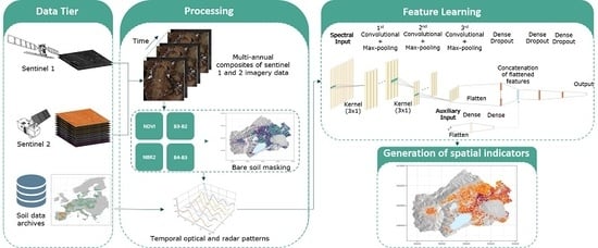
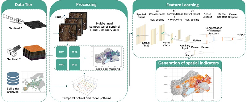
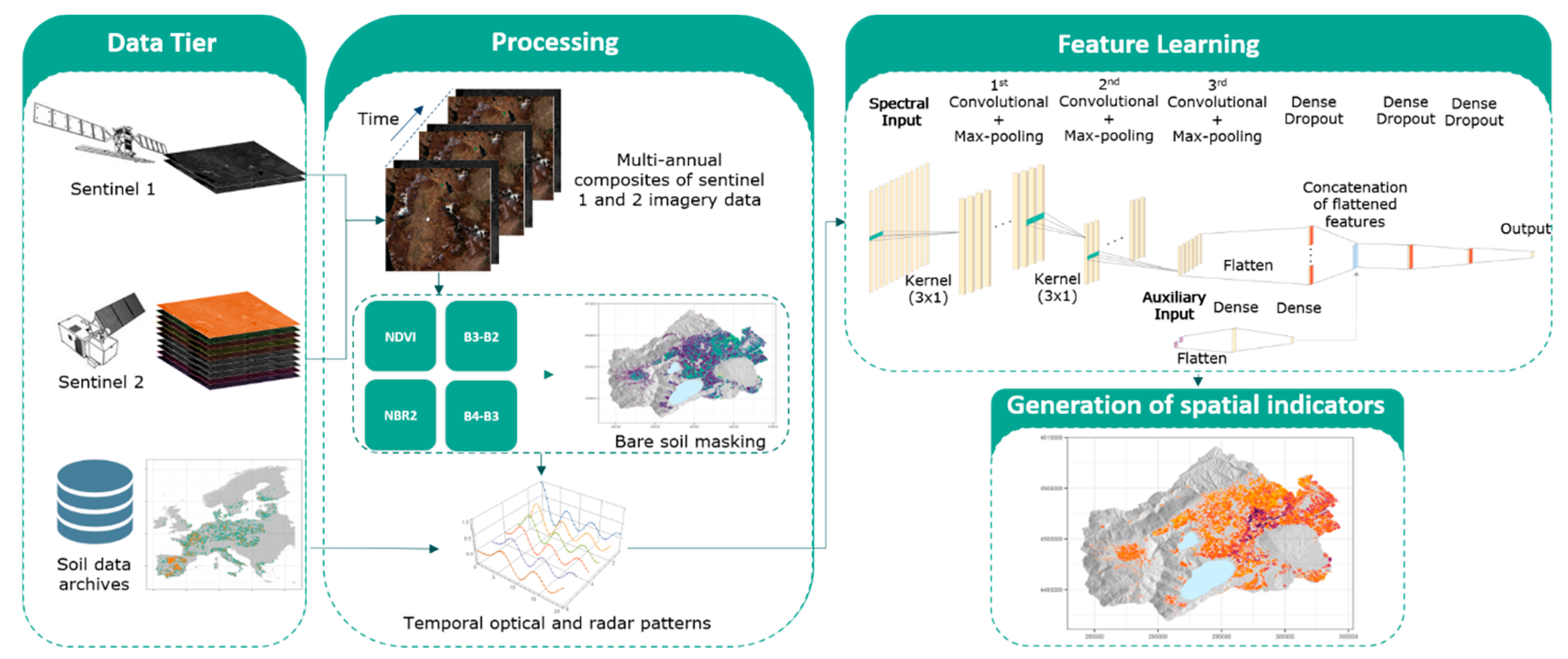
2.3.1. Convolution Neural Network for Soil Attributes Mapping

Previous works indicated great potential in utilization of non-linear machine learning methods for quantification of soil attributes with reflectance values and complementary covariates of multispectral EO platforms. Mainly, these studies focused on the information derived from the median spectral values of satellite products, without taking into account the temporal variability of the Earth’s surface such as soil moisture and roughness. Our choice for the incorporation of new deep learning techniques, such as CNN, was motivated by our goal to evaluate the complementary information of inter- and intra-annual spectral variations in the chemometric modeling. These algorithms are considered very effective to derive features from short segments of the overall spectral signals [27]. Readers unfamiliar with the CNNs may refer to recent studies [9,28] and relevant reviews [29] where 1D-CNN basic features and operations are described. In addition, a glossary related to deep learning terminology is provided in the end of this manuscript to further explain specific terms that support the description of the CNN model in the following paragraphs.

Here we present the network architecture of the proposed multi-input CNN, which aims to predict topsoil clay content based on the remotely sensed imagery data. The proposed approach leverages the techniques of 1-D CNNs to estimate clay content using in conjunction as predictors (i) all the selected 1-D spectral signatures of masked bare soil pixels (Sentinel-2 10 bands), (ii) their closest, in terms of date, combined observations from VV and VH data (additional two bands), and (iii) the geographical coordinates for each sample point across the observation time. This spectral information, both radar and optical values, is seen by the network as a single entity for each observation date, while the multiple observations within the years captured the related introduced uncertainties (e.g., decorrelation effects through temporal environmental factors). Thus, the end goal is to combine the potentially complementary information arising by the variations of these values.

The proposed network is arranged in a series of six different types of layers, namely: (i) the input layers, where the remotely sensed values accounted for constitute the spectral input channel and the geographical coordinates the auxiliary input channel; (ii) the convolutional layers, which filters a given input and extracts information from specific spectral regions by carrying out the convolution operation; (iii) the pooling layer, used to reduce the resolution of the temporal dimension; (iv) the flattening layer, which converts the multi-channel filters into a single continuous vector; (v) the dense layer, which connects all outputs of the previous layer to all inputs of the forthcoming layer; and (vi) the concatenate layer, which takes as input the resulted tensors from spectral and auxiliary input and returns a single tensor. Figure 4 depicts the overall network architecture. To train the network, we employed the Adam optimizer [30] using a batch size of eight while the number of epochs are set to 100. Most notably, were are not interested in identifying the temporal trends in the spectral signatures per se, considering that the texture of the soil samples remains unaltered within the span of few years. Thus, the convolution occurs across the spectral dimension and not the temporal one.

More concretely, first, a 1-D convolutional layer with 16 filters convolves the spectral input (12 channels), utilizing a kernel of size three. Then we applied a second 1-D convolutional layer that comprised of 64 filters with a kernel size of three. Each convolutional layer was followed by a rectified linear unit (ReLU) activation layer. The convolved layers of the CNN were flattened and then fully connected by a dense layer, followed by a dropout layer with a rate of 0.5. For the dense layer, an exponential linear unit (eLU) activation function was selected, whilst a kernel regularizer 0.002 was used to penalize the weights and reduce overfitting. In order to reduce the dimension of the data (50% each time) we applied a max pooling layer after the convolutional layers. Considering the auxiliary input (two channels, namely the latitude and longitude) two dense layers were used. The first dense layer had eight outputs, and the second dense layer had four outputs. The results of the spectral and auxiliary inputs were then combined whereby a concatenation layer was established. Subsequently, two dense layers of 64 and 16 channels, respectively, applied with an eLU activation function and a kernel L2 regularizer of 0.002. Both were followed by the application of a dropout layer (0.2). Finally, we concluded with one output layer of size one, which corresponded to the target variable, using the tanh activation function.

The layers are also presented in

Table 3. Description of the layers used in the multidimensional convolutional neural network (CNN) architecture.

Type	Kernel Size (Channels × Width)	Filters	Channels	Width	Activation
Spectral input	-	-	12	150	-
Convolutional	3 × 1	16	10	150	ReLU
Max-pooling	1 × 2	-	-	75	-
Convolutional	3 × 1	64	8	75	ReLU
Max-pooling	1 × 2	-	-	37	-
Convolutional	3 × 1	16	6	37	ReLU
Max-pooling	1 × 2	-	-	18	-
Flatten	-	-	-	1728	-
Dense + Dropout	16	3	-	8	eLU
Auxiliary input	-	-	-	2	-
Dense	-	-	-	8	-
Dense	-	-	-	4
Concatenation	-	-	-	-	-
Dense + Dropout	-	-	-	64	eLU
Dense + Dropout	-	-	-	16	eLU
Flatten	-	-	-	1	tanh

.

2.3.2. Model Interpretability of CNN

Model interpretability is crucial in order to understand what computations are performed at each layer in CNN. To our knowledge limited studies exploit techniques to gain valuable insights. In this context, appropriate techniques have developed to analyze the preferred inputs of each filter [31] and their applications allow us to derive meaningful interpretations in the domain of soil spectroscopy. A summary of them may be found in Zhang et al. [32].

To understand how the model derives its predictions a post-hoc explainability analysis was conducted. This is an important step in order to make the system more interpretable [33] and ensure the robustness of the predictions, in accordance to the principles of explainable artificial intelligence [34]. To this end, we examined the generated feature maps of the final convolutional layer, which takes into account only the spectral and radar information (and ergo not the location of the samples). For each feature map, the top 5% (in terms of activation) of the patterns from the training set were identified, and their input features and respective clay content were visualized.

2.3.3. Competing Modeling Approaches and Additional Experiments

To compare the accuracy of the proposed multidimensional CNN we also tested the performance of RF and of a different ANN architecture, as representative approaches of the current state-of-the-art. Previous work of Demattê et al. [19] was used as the benchmark. In that regard, we produced the median spectral reflectance of the Sentinel-2 bands to assess the performance of the competing algorithms based on the temporal synthetic spectral reflectance profile of each soil sample.

RF is an ensemble learning classifier [35] that has achieved good performance metrics in various soil spectroscopy studies [36,37]. An appropriate tuning of hyperparameters ensures the RF’s consistency. Thus, a grid search on a five-fold cross-validation experiment was conducted to select the optimal hyperparameters for RF model. In particular, we selected the number of variables that can be sampled in each split of the trees from {6, 24} and the minimal number of samples for the terminal nodes from {5, 10, 20, 50}, while the tree parameter were selected from {500, 1000, 1500}. Finally, the optimal set of hyperparameters is as follows: 24 and 20 for the first and second parameter and 1000 number of trees, for the RF and 22 and 50 for the first and second parameter, respectively and 1000 number of trees, for the RF without the location information.

Similarly, we created an ANN architecture using as input (i) the median temporal synthetic spectral reflectance profile of each soil and (ii) the median values along with the geographical coordinates of each sample. Briefly, this network consisted of four trainable layers. The first layer contained eight units. Then we applied a second dense layer, which comprised of 32 units, followed by a dropout layer with a rate of 0.2. For the second dense layer, an eLU activation function was selected, whilst a kernel regularizer L2 of 0.002 was used. In addition, we had another dense layer with eight units and the same parameters as the previous one. We concluded with one output layer of size one, which corresponds to the target variable, using the tanh activation function.

Furthermore, additional experiments were performed. We evaluated the performance of RF and ANN including also the data from Sentinel-1 for each time step and not solely the median reflectance values of the multispectral bands to statistically compare their predictive performance with those derived from the proposed 1D-CNN. Moreover, the proposed CNN model was trained and tested without the use of SAR data, as well as without the use of SAR and geographical coordinates.

2.3.4. Dataset Partition

The averaged spectra on a per pixel basis of Sentinel-2 values for each of the selected samples from the LUCAS database were used to partition the samples into calibration (4901) and testing (1235) set (Figure 5a), uniformly by the Kennard–Stone algorithm [38], so that the calibration set was distributed evenly based on spectral representativeness, extending among the EU territory, as illustrated in Figure 5. We performed bootstrap aggregation without replacement where five different sets of size 3920 (i.e., 80% of the 4901 calibration data) were used to each train a separate model and predict on the test set. Then, these results were combined by averaging the output and thus producing a single prediction for each testing datum. This procedure was performed for all the algorithms, CNN, RF, and ANN. Finally, to test the CNN model the 52 samples from the Zazari river basin were utilized as an independent test dataset.

2.3.5. Evaluation of the Models

In order to assess the performance of calibration models for soil clay content we calculated the root-mean-square error (RMSE, Equation (1)), the coefficient of determination (R², Equation (2)), and the ratio of performance to interquartile range (RPIQ, Equation (3)). The equations used were as follows:

$$\mathrm{RMSE}=\sqrt{\frac{{\sum }_{i=1}^{i=N}{\left(y_i-\widehat{y_i}\right)}^2}{N}}$$

(1)

$${\mathrm{R}}^2=1-\frac{{\sum }_{i=1}^{i=N}{\left(y_i-\widehat{y_i}\right)}^2}{{\sum }_{i=1}^{i=N}{\left(y_i-\overline{y}\right)}^2}$$

(2)

$$\mathrm{RPIQ}=\frac{\mathrm{IQ}}{\mathrm{RMSE}}$$

(3)

where $y_i$ is the observed value and $\widehat{y_i}$ is the predicted value of sample i, N the number of observations (Equation (1)), $\overline{y}$ is the mean of the observed values (Equation (2)), and IQ is the interquartile range (IQ = Q3 − Q1) of the observed values (Equation (3)). Q1 and Q3 denote the first and third quartile, respectively.

2.4. Implementation

Our approach was implemented in a way such that Sentinel-1 and Sentinel-2 data handling were processed using the scalable capabilities of GEE [39], making the whole processing routine distributed and thus more computationally efficient. The coordinates (WGS84) of the soil sample sites were imported into GEE using Google fusion tables. The spectral signatures corresponding to the sample sites were then extracted and downloaded for further processing in a local environment. The statistical and CNN regression analyses were performed utilizing the R software [40], with the keras package [41]. The caret package [42] was also used for the development of the RF model. The models were built on a workstation with a NVIDIA Quadro K4200 graphics processing unit.

3. Results

3.1. Times Series Preliminary Analysis

The multi-temporal analysis of bare soil reflectance of LUCAS sampling sites implemented in this study extended from January 2017 to December 2019. Our choice to focus on a three year study was mainly based on the need to provide a sufficient number of scenes for statistical analysis, able to capture the clean soil spectrum (i.e., without cloud coverage or presence of dry and green vegetation) each sample site at least once. It should be noted that the distribution of cloud-free scenes was significantly variable for different parts in the European continent, having an impact on the number of time pixels were exposed (i.e., more clean soil pixels in Mediterranean countries compared to Northern Europe).

Overall, there were a total of 21,334, 48,913, and 45,842 bare soil pixels in 2017, 2018, and 2019 (the Sentinel-2 Level 2 were ingested in GEE from 2019 and backwards), corresponding to 4507, 5659, and 5397 extracted points, respectively (Figure 6). Then, a time series of each soil site sample with 10 spectral bands was generated. For the majority of pixels (96%) at least two cloud free observations were available in this period and about a quarter of the pixels had more than 25 observations available. Approximately 15% of the pixels had less than four cloud-free recordings during the entire study period.

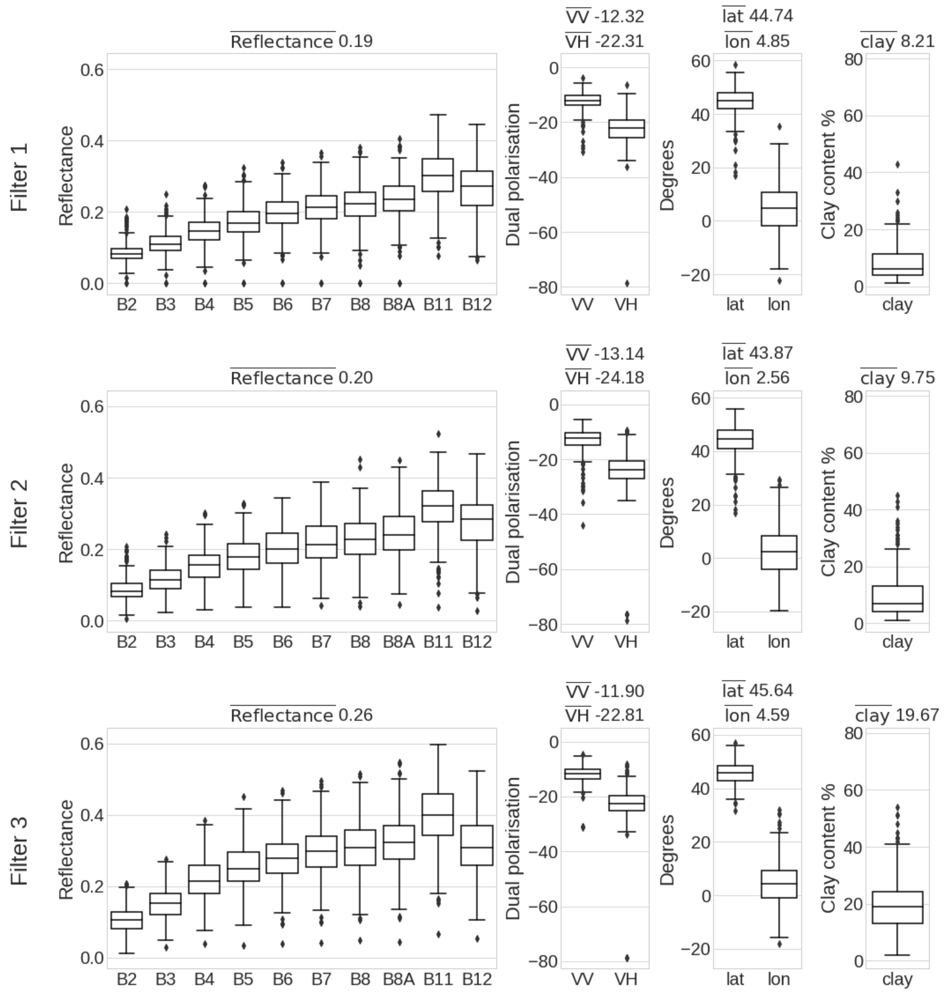
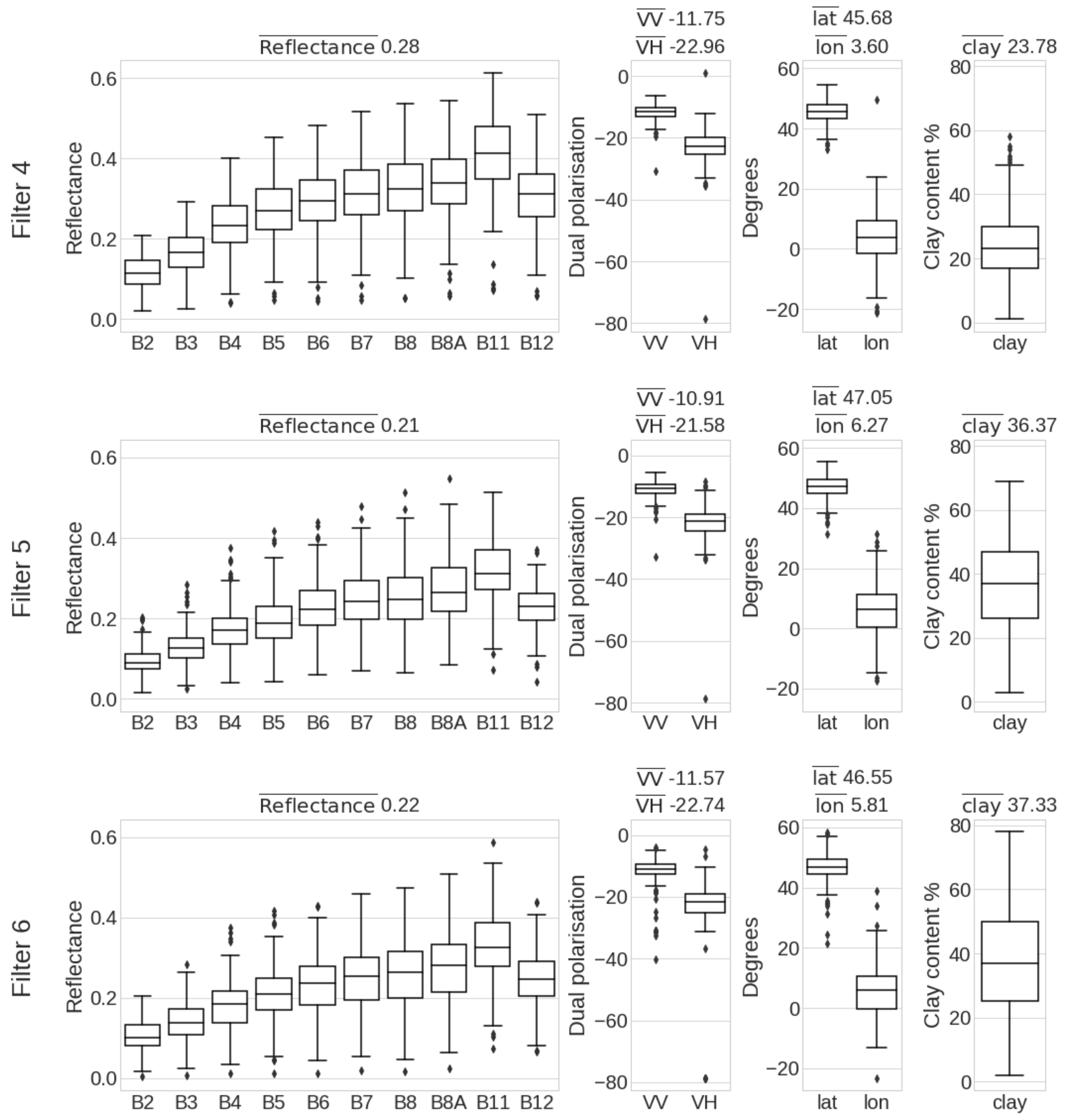
3.2. Bare Soil Spectral Pattern from LUCAS and Sentinel-2 Data

The next steps in our data analyses were performed using the LUCAS soil sampling points that were masked out as bare soil pixels. Then, for each selected soil sampling point the median absorbance spectral response as well as the associated standard deviation among all the MSI Sentinel-2 recordings was calculated (Figure 7). For comparison we also resampled and converted to reflectance values the corresponding laboratory LUCAS spectra to Sentinel-2 bands. Overall, we could observe that the position and the shape of Sentinel-2 and resampled LUCAS spectral signatures present noticeable differences (e.g., albedo). In particular, the resampled laboratory spectral signatures indicated higher reflectance values relative to MSI Sentinel-2, since the measurement were performed in a controlled environment and not influenced by the surface conditions of the open fields (e.g., roughness caused by the particle size and soil moisture). Moreover, this variation was expected since we should consider that LUCAS SSL was made in disturbed soil samples, while in real field conditions the soil surface were in an undisturbed condition.

Examples of variation of spectral signatures taken from the Sentinel-2 bare soil images for representative LUCAS sites are illustrated in Figure 8. Examples correspond to clay, sandy, silty and silty clay soil type [43]. The number of pixels masked out as bare soil was different depending on the region. For example, at points characterized as clay, sand, silty and silty clay we created a time series of 16, 22, 29 and 18 stacked pixels, respectively. Hence, the illustrated trajectories correspond to the associated number of selected observations across the period of 2017–2019 for the 10 Sentinel-2 bands.

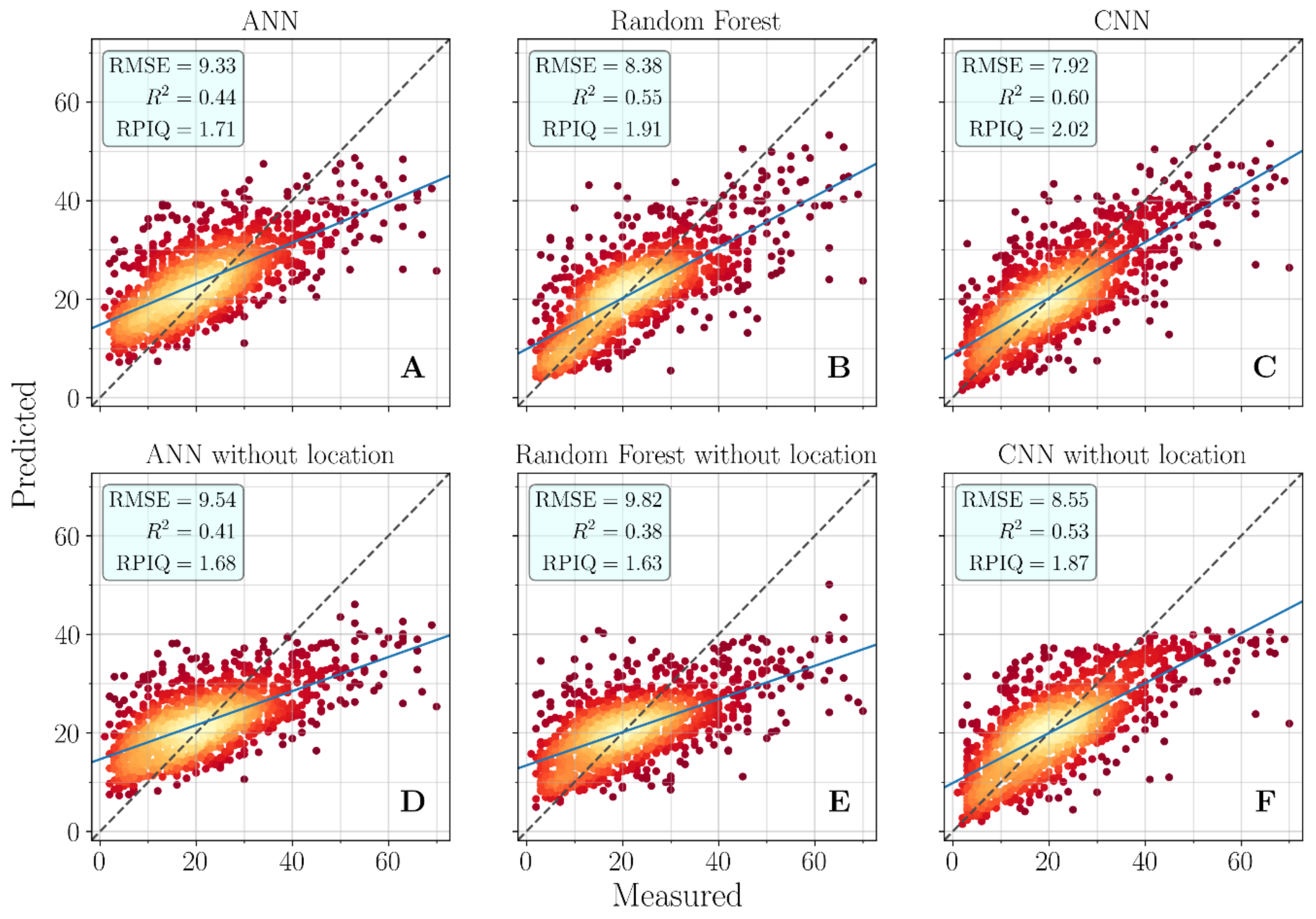
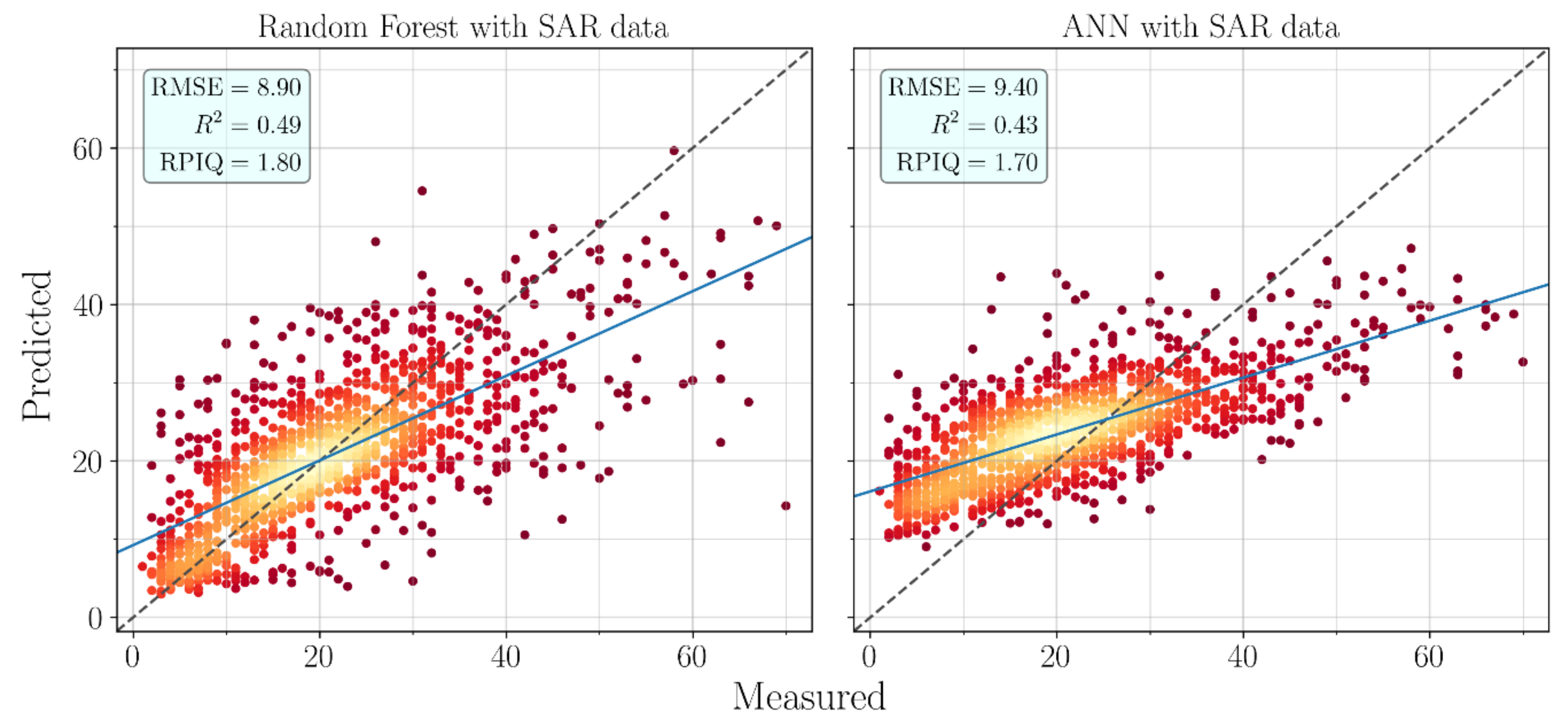
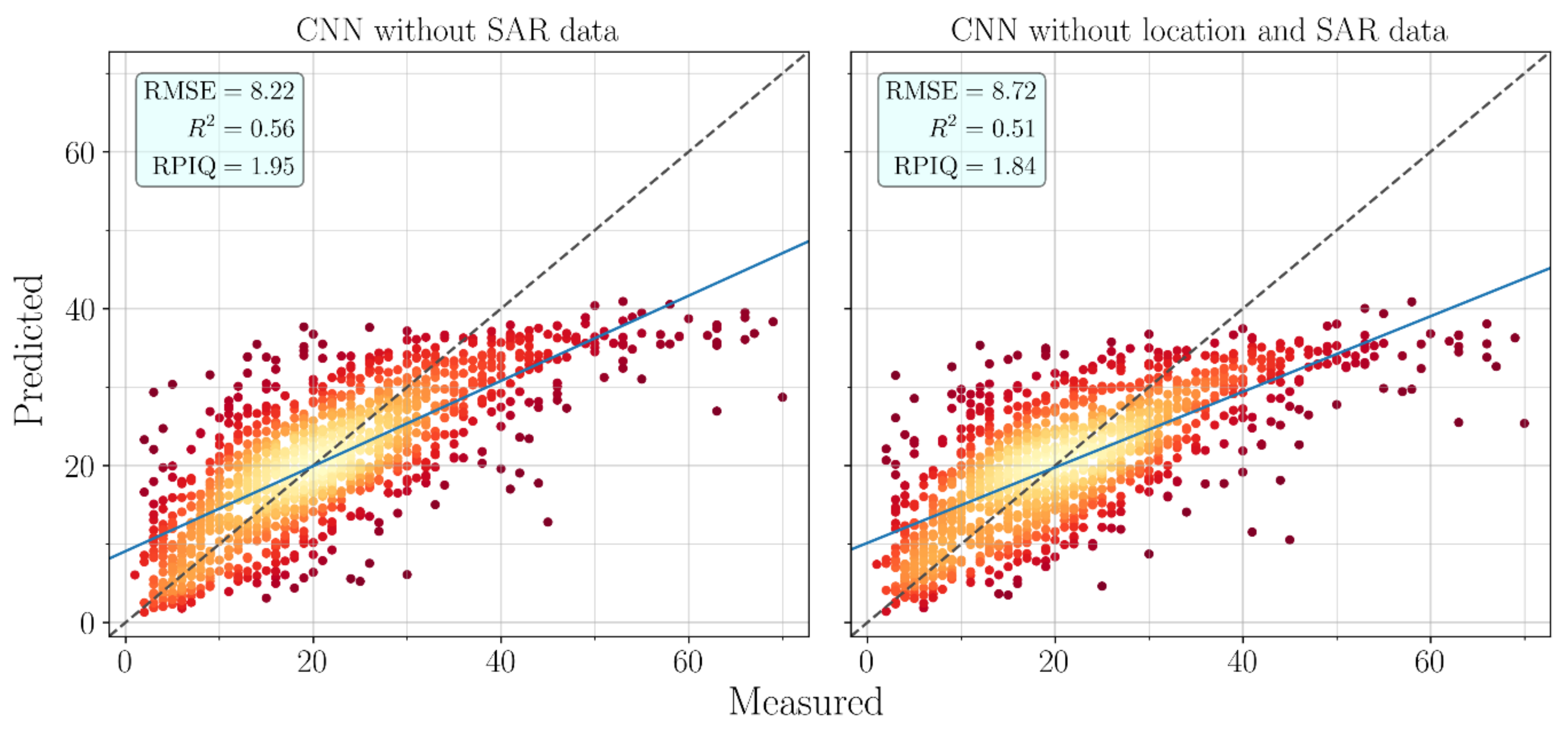
3.3. Prediction Performance

The results of the CNN model for the prediction of clay content across the soil samples of the LUCAS database and the best models from the competing approaches are presented in Figure 9.

It should be noted that the CNN model leveraged a plethora of input features attaining a performance of RPIQ 2.02 and R² = 0.60, a notable result (Figure 9C). This shows the multi-input architecture’s potential to combine effectively the complimentary information contained in the pool of both optical and radar spectral information and those from auxiliary geographical coordinates. Therefore, in comparison with the prediction performance values of the competing algorithms the CNN model significantly improved the performance predictions (R² = 0.55, RPIQ = 1.91 and R² = 0.44, RPIQ = 1.71, Figure 9A,B) and decreased the RMSE by a relative 4.5% and 6.5% to RF and ANN, respectively. Hence, the effect of the synergistic use of optical and SAR data was evident, since the most accurate models were developed from the integration of both inputs in the proposed CNN model compared to both RF and ANN models that used the entire Sentinel-1 and Sentinel-2 dataset or simple the median values of Sentinel-2. Moreover, the results indicate that each model has increased its performance with the inclusion of geographical coordinates as auxiliary features. Considering the additional information derived from geographical coordinates, we could observe that it slightly improved (5.5% decrease in RMSE) the CNN’s prediction of the soil clay content compared to the CNN without the auxiliary input layer (R² = 0.53 and RPIQ = 1.87, Figure 9F). However, the improvement due to additional geographical variables was more pronounced for the RF model, indicating that it did not sufficiently exploit the spectral information (R² = 0.38 and RPIQ = 1.63, 9E). A significant improvement of 4% was recorded with the ANN model compared with the version without the location information (R² = 0.41 and RPIQ = 1.68, Figure 9D). Overall, even if the improvement of prediction is very slight, it can be expected that complementing the models with auxiliary input features capturing the spatial characteristics of the soil samples enable more precise prediction of topsoil clay content. To conclude, in all the cases the CNN model outperformed the competing modeling approaches, as illustrated in Figure 9, where the results are given. Finally, the corresponding results and the associated scatter plots from the additional analyses are given as Appendix A and Appendix B.

3.4. Interpretability of the Multi-Input CNN Model

The post-hoc explainability analysis that we performed enabled us to understand which groups of patterns and consequently which features each feature map identifies and considers as important for the prediction of the target property. Out of all generated feature maps, we selected six representative filters to assist in the interpretation of the model (Figure 10 and Figure 11).

Since it is difficult to infer what the deep features depict by directly visualizing their values, the visualization propagates back to the initial features, which are more interpretable and depicts in the form of boxplots, per each filter, the reflectance spectra, the polarization, the location, and the clay content. For visualization purposes, the filters were ordered according to the average clay content of their top 5% activated samples, and the corresponding input features were unnormalized in order to be expressed in their original units. The first two filters detect “low” clay content (i.e., with values mostly between the minimum and Q1), the second two “medium” clay content (i.e., with values at Q2), while final the two last filters predict the “high” contents (i.e., at about Q3 and beyond). This is an interesting result suggesting that the CNN had untangled the latent information and developed complex features, which could identify the clay content only using the spectral and radar information.

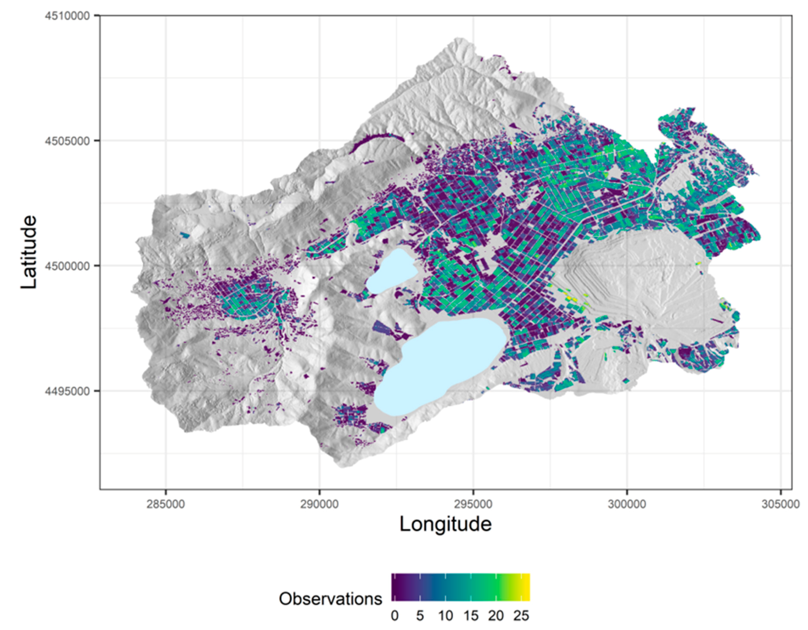
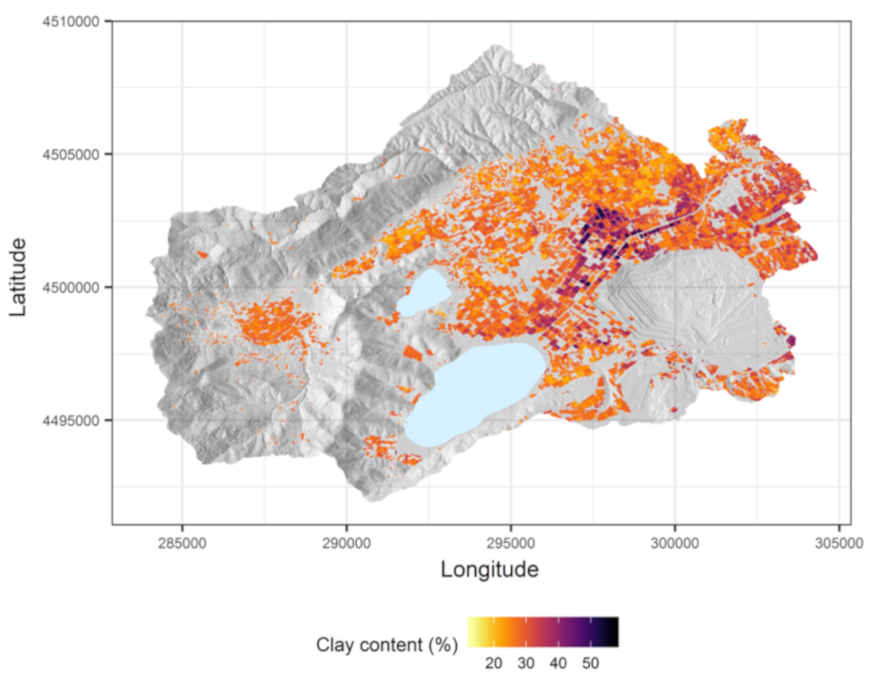
3.5. Surface Mapping of Soil Attributes

In this case, S2MoS was implemented using EO images from 25 distinct dates, well distributed across the agricultural calendar, acquired over a period of two years over the Zazari test site. Using the predefined 0.25 and 0.075 threshold values for NDVI and NBR2, respectively, we extracted 72.12% bare soil pixels over the agricultural fields, as illustrated in Figure 12.

So, once the CNN model was validated (see Section 3.3), it was directly applied to the selected bare soil pixels for all of their temporal observations (Sentinel-1 + Sentinel-2), which represents situation’s information of the soil surface across different periods (wet, tillage, ploughed, etc.) in the Zazari river basin. At the scale provided, the results were visually homogenous and free of any apparent artifacts, mainly due to the number of pixels masked as bare soil varies depending on the region. The resulting map (Figure 13) illustrates the parcel level soil clay content as derived by the proposed CNN model. The predicted clay values using the proposed CNN model showed relatively similar patterns with the areas covered by the different soil classes (Figure 2a). Moreover, we had an underestimation of the higher clay content, resulting to a moderate predictive performance (R² = 0.51, RMSE = 19.8%), compared to the ground truth 52 points.

4. Discussion

The S2MoS proposed in this research has proved its capability to attain better prediction performance metrics compared to the current state-of-the-art approaches. These results were attributed to the multi-input CNN architecture, which has enabled us to leverage the complementary information contained among reflectance and radar values, as well as the geographical information of each sample. In this section we discussed whether the objectives of this research were achieved (Section 4.1), as well as we evaluated the interpretation of the way that input and relevant output associations was modeled (Section 4.2). We also compared the findings of this paper with existing literature (Section 4.3) and suggest directions for future research (Section 4.4). Finally, in Section 4.5, we provided insights and recommendation for the development of a global and operational EO-based soil monitoring system.

4.1. EO Regression Analysis with the Use of Convolutional Neural Networks and Synergistic Use of Optical and SAR Data

Currently, EO-based soil spectroscopic regression analysis mainly focuses on machine learning models [36,44] and recently on one-dimensional spectral signature processing with deep learning techniques [45]. Following a growing trend in the application of deep learning techniques in multidimensional prediction on various Earth system science problems [46], we employed a new multi-input approach of spectroscopy analysis using a CNN model, which takes into account both the spectral and radar characteristics of exposed soil sites, across multiple observations, for mapping their spatial characteristics. Those studies have used the Landsat archive to extract bare soil spectral signatures over large areas. To the best of our knowledge, such an investigation has not yet been thoroughly examined for Sentinel optical data. The latter data offer enhanced spatiotemporal resolution compared to Landsat imagery, making them advantageous for producing high resolution soil spatial explicit indicators on large scales. Unlike the proposed S2MoS, none of the above data mining approaches have previously examined leveraging multiple observations as a single entity. Until now, multi-temporal approaches generated outcomes reflecting the median value of the available observations. The proposed S2MoS enables a multi-temporal analysis, which efficiently can leverage information from the temporal behavior in top-soil across the years (Figure 8). This was introduced here for the first time and was the cornerstone of the proposed framework.

Τhe use of Sentinel-2 bands was further supported, by integrating radar values as supplementary predictors. Consequently, a considerable expansion of the feature space (considering both temporal and spectral dimensions) was created, which could not be efficiently handled by the current machine learning approaches. Although the RF algorithm can be considered as a successful approach to soil texture classification [36,37], the proposed CNN network has proven to have significant advantages over other methods used in the EO-based soil spectroscopic regression analysis with respect to prediction performance (R² = 0.60, RPIQ = 2.02). In particular, this approach demonstrates a significant improvement in overall accuracy compared to the competing machine learning methods that make use of the multi-year optical composite (i.e., the median) as indicated in Figure 9. Furthermore, as it is expected, the proposed CNN produced the best results even when the RF and ANN models were trained in the whole dataset (see Appendix A). This scenario demands a long training time for few thousand points considering geographical coordinates, optical, and SAR imagery data as input values. The importance of the proposed CNN architecture can be further highlighted by a set of additional comparisons that were performed using as predictors the spectral source without the use of supplementary predictors (i.e., radar values). The corresponding results are given in Appendix B, where in all cases the integrated information of SAR data increases the overall predictive performance. Accordingly, it was concluded that the complementary SAR observations are very useful for improving overall accuracy by capturing the spectral influence of soil moisture and roughness of soil exposed pixels. This finding is also highlighted by Bousbih et al. [15], where they retrieved soil roughness levels and accounted them in soil texture classification.

4.2. Feature Importance

The proposed CNN allows a degree of interpretability enabling the identification of key spectral regions in accordance to the principles of explainable artificial intelligence [34]. By visualizing the selected filters from the feature maps (Figure 10 and Figure 11), the following observations can be made: (i) the albedo of the samples tends to increase as the clay content increases, but at high concentrations it decreases again; this is in accordance with the observations made from the laboratory spectra of the air-dried samples [47], (ii) although the coordinates’ distributions are mainly influenced by the high presence of samples in central Europe, a trend can be identified in that samples with higher clay content are to be found in higher latitudes; this is in accordance with the identified correlation between them, which the CNN identified only though the spectral and radar information, (iii) there is a noticeably larger absorption in band B12 as the clay content increases; again, this complies with the well-reported observation that absorbances around 2.2 and 2.3 μm are due to the presence of OH in the mineral structure [48]—this is a region that may also affected by the presence of soil organic matter, as well as CaCO₃, whose content however is low in the European croplands [21], thus its effect is not profound, (iv) VV tends to be more sensitive in the changes of the average clay content, as it is more affected than VH by the changes in soil roughness, which may be at least partially caused by the different soil texture [16], (v) large clay contents (i.e., larger than Q3) are harder to identify as the generated feature maps evidently confound them with lower concentrations. These interpretations have made the reasoning process of the model more transparent; they indicate how the model has obtained a clear mapping between the predictors and the output property, albeit not an infallible one, with a distinct physical meaning.

4.3. Comparison with Current State-of-the Art Regression Algorithms

Several studies [36,37] have assessed the potential of Landsat archive imagery data to the map surface clay content, finding satisfactory–good results (0.63 < R² < 0.75). Recently, Gholizadeh et al. [14] and Vaudour et al. [12] evaluated Sentinel-2 images for soil surface properties estimation. In the aforementioned studies, the soil attributes from the surface layer were modeled using machine learning techniques, where each pixel was enriched by some additional features coming from combinations performed among the extracted band values [14,49]. Herein, there is no need to include additional covariates in the model, as convolutional layers ensure that deep features are automatically constructed. Moreover, most studies in EO spectroscopic analysis calibrate multivariate regression models based on reference samples from their study area. In this research, the number of observations in the calibration dataset was restricted to LUCAS data, in contrast to current approaches. Liu et al. [45] also used existing SSLs to develop models for estimation of topsoil clay content and later generated relevant maps based on hyper-spectral image and a transfer function. In their approach, a few field samples and relevant spectral signatures were utilized to fine tune the calibration of model, resulting in a model with R² around 0.6. However, we should mention a typical extrapolation problem in digital soil mapping, since very often the developed models perform quite well in training and even test datasets but deviate strongly for data outside their valid area. In that regard, the lower performance in the Greek (R² = 0.51) test area (Figure 13) can be explained by the availability of only one LUCAS soil sample within the Greek study area or by the fact that current samples are not representative of the soil variability of the other regions.

4.4. Perspective of Embedding New Reference Soil Databases and Additional Spectral Information

Even though soil texture can be considered constant for more than 20 years, several changes can be potentially caused by natural or anthropogenic activities affecting the reflectance in VNIR–SWIR. This is more prominent for other soil parameters such as organic carbon. In that regard, our approach should be extended to explore more soil properties, such as soil organic carbon, by leveraging the more recent LUCAS topsoil database of 2015 that covers a time period when the Sentinel satellites were operational. Moreover, LUCAS was designed as a monitoring system and not as a mapping tool, hence we should take into account the feature space in the design of sampling strategies [50] in order to develop more reliable calibration models. Finally, it should be noted that further analyses should be performed for assessing precisely temporal spectral variations, e.g., through temporal changes of the soil moisture and/or roughness and appropriate parametrization should be performed to effectively combine SSLs and EO data.

Additionally, by the combination of reflectance data and EO-based terrain or land use derivatives [8,36], we expected to overcome the limitations of Sentinel-2 spectral resolution in key ranges of the electromagnetic spectrum. Furthermore, the S2MoS scheme described herein may be applied to combine other heterogeneous sources in a similar fashion. For example, spectra from the VNIR–SWIR and the thermal infrared range where some of the fundamental vibrations take place, as demonstrated in Chabrillat et al. [51] and Notesco et al. [52] may be appropriately combined to yield better performance than the one attained. In this manner, although Sentinel-2 data has spectral bands similar to Landsat 8’s, it excludes the thermal infrared sensor. However, its capability to obtain a large number of images allows the retrieval of more information and the calibration of robust models. This is an important fact when considering the differences in models’ performance between Landsat estimations and those from Sentinel-2, like the current research.

4.5. Towards an EO-Based Soil Monitoring System

This section highlights the current limitations, discusses potential solutions that reinforce the rationale that remote sensing, artificial intelligence, and digital soil mapping communities should work closely together to better understand and eventually overcome the challenges for an EO-based soil monitoring system.

Copernicus data can be considered as a key resource but the need for higher spatial resolution optical and SAR, as well as hyperspectral and thermal space-based observations can be the game changers for an operational EO-based soil monitoring system. The forthcoming Copernicus Hyperspectral Imaging Mission (CHIME), NASA Surface Biology and Geology (SBG) mission, and Copernicus Land Surface Temperature Monitoring (LSTM) may close this gap and fulfill these needs in them of spectral resolution and thermal coverage, respectively. In future studies, it is worthy to investigate how we can properly integrate satellite soil moisture retrievals and fuse them with multispectral bands for soil mapping. It has been proven that data from Sentinel-1 can be used to define operational schemes and identify synergies, allowing for observational methods of soil moisture to be further evolved and for tailored algorithms delivering mature products to be developed based on our proposed methodology [53]. Synergies with Landsat or the existing hyperspectral sensors in orbit (e.g., PRISMA from Italian Space Agency) should be prioritized to assess the limitations whereby standalone multispectral Sentinel-2 data is not sufficient to reach the desired spatiospectral reliability [54].

The proposed deep learning CNN paves the way to overcome many of the limitations that have, until now, hindered a more wide-spread adoption of artificial intelligence in the domain of soil spectroscopy, such as multiple kernel learning approaches [55] and interpretable fuzzy rule based algorithms. This kind of models are transparent in terms of their reasoning process, thus enabling experts alike to holistically address the issues tackled in contrast to black box models. In future studies, the application of generative adversarial networks [56] for regression should be prioritized, since the use of generator and discriminator networks can be a powerful tool for the synergistic used of large SSLs and space-borne data. In that regards, unlike on LUCAS, Global [57], and GEOCRADLE SSLs [58], large, reliable, labeled soil data do not always exist in soil science, not only because of the sizes of the datasets involved, but also owing to the absence of standard operating procedures in chemical laboratory measurements, as well as common guidelines on lab spectroscopy measurements to ensure interoperability and reliable reusability. The upcoming release of LUCAS version of 2015 as well as new efforts in Africa and Latin America based on agreed set of harmonization principles will allow us to have better chance of chemical attributes estimation within an intra-annual calibration of models.

It should be noted that, approaches based on synergistic use of multimodal EO data, including the available hyper-spectral missions [59], can further raise computational challenges dealing with petabytes of data. To that end, it is critical to exploit the existing IT capabilities of cloud computing and processing platforms, such as GEE, DIAS, and Committee on Earth Observation Satellites Data Cube [60], to significantly reduce the time needed to process EO information.

5. Conclusions

This paper proposed a topsoil clay content quantification technique based on a multi-input deep convolutional network and a multi-temporal analysis of optical and radar imagery data to produce detailed soil maps of high spatial coverage over agricultural regions. Our approach was implemented with Sentinel-1 and Sentinel-2 data using data from 6136 agricultural sites of the LUCAS SSL, over a three-year period. A detailed study was conducted in the Zazari river basin in Northern Greece to independently examine the performance of the model and allow for better visualization. For that purpose, we used soil data from 52 sites collected within a study period extending from August 2018 to September 2019.

The results deliver preliminary insights of the potential of the integrated optical and radar time series products that can be used for topsoil mapping. In particular, our novel methodological framework can efficiently utilize both Sentinel-1 and Sentinel-2 information instead of solely the median spectral reflectance of each sample. The proposed technique shows promising results (R² = 0.60, RPIQ = 2.02) comparing favorably against current state-of-the-art data mining procedures to produce accurate soil predictions from satellite images. Optical and radar bands play different roles in EO-based soil monitoring and integrating the relative utility of these bands is an effective way to enhance the regression performance. In that regard the proposed approach shows that the synergistic use of SAR and optical remote sensing could facilitate the provision of useful added value information regarding the effect of ambient factors of exposed soils, achieving an improvement of 5.5% in RMSE over the performance of the RF, as the best model, which used as input solely the synthetic spectral reflectance of each sample. Moreover, the information based on additional auxiliary input (e.g., geographical coordinates) is an effective complementary source of information to enhance the prediction performance by considering the spatial relationship between regions and soil characteristics. Although this approach has been developed and tested on MSI Sentinel-2 imagery data, its potential and capability can be adopted on the forthcoming hyperspectral orbital sensors where better results are expected, and more soil attributes could be predicted accurately.

References

1. Montanarella, L.; Pennock, D.J.; McKenzie, N.; Badraoui, M.; Chude, V.; Baptista, I.; Mamo, T.; Yemefack, M.; Aulakh, M.S.; Yagi, K.; et al. World’s soils are under threat. SOIL 2016. [Google Scholar] [CrossRef] [Green Version]
2. Dai, Y.; Shangguan, W.; Wei, N.; Xin, Q.; Yuan, H.; Zhang, S.; Liu, S.; Lu, X.; Wang, D.; Yan, F. A review of the global soil property maps for Earth system models. SOIL 2019, 5, 137–158. [Google Scholar] [CrossRef] [Green Version]
3. Wulder, M.A.; Masek, J.G.; Cohen, W.B.; Loveland, T.R.; Woodcock, C.E. Opening the archive: How free data has enabled the science and monitoring promise of Landsat. Remote Sens. Environ. 2012, 122, 2–10. [Google Scholar] [CrossRef]
4. Hengl, T.; De Jesus, J.M.; Heuvelink, G.B.M.; Gonzalez, M.R.; Kilibarda, M.; Blagotić, A.; Shangguan, W.; Wright, M.N.; Geng, X.; Bauer-Marschallinger, B.; et al. SoilGrids250m: Global gridded soil information based on machine learning. PLoS ONE 2017, 12. [Google Scholar] [CrossRef] [Green Version]
5. Behrens, T.; Schmidt, K.; MacMillan, R.A.; Viscarra Rossel, R.A. Multi-scale digital soil mapping with deep learning. Sci. Rep. 2018, 8. [Google Scholar] [CrossRef] [Green Version]
6. Padarian, J.; Minasny, B.; McBratney, A.B. Using deep learning for digital soil mapping. SOIL 2019, 5, 79–89. [Google Scholar] [CrossRef] [Green Version]
7. Wadoux, A.M.J.-C.; Padarian, J.; Minasny, B. Multi-source data integration for soil mapping using deep learning. SOIL 2019, 5, 107–119. [Google Scholar] [CrossRef] [Green Version]
8. Behrens, T.; Schmidt, K.; MacMillan, R.A.; Viscarra Rossel, R.A. Multiscale contextual spatial modelling with the Gaussian scale space. Geoderma 2018, 310, 128–137. [Google Scholar] [CrossRef]
9. Tsakiridis, N.L.; Keramaris, K.D.; Theocharis, J.B.; Zalidis, G.C. Simultaneous prediction of soil properties from VNIR-SWIR spectra using a localized multi-channel 1-D convolutional neural network. Geoderma 2020, 367, 114208. [Google Scholar] [CrossRef]
10. Angelopoulou, T.; Tziolas, N.; Balafoutis, A.; Zalidis, G.; Bochtis, D. Remote Sensing Techniques for Soil Organic Carbon Estimation: A Review. Remote Sens. 2019, 11, 676. [Google Scholar] [CrossRef] [Green Version]
11. Castaldi, F.; Hueni, A.; Chabrillat, S.; Ward, K.; Buttafuoco, G.; Bomans, B.; Vreys, K.; Brell, M.; van Wesemael, B. Evaluating the capability of the Sentinel 2 data for soil organic carbon prediction in croplands. ISPRS J. Photogramm. Remote Sens. 2019, 147, 267–282. [Google Scholar] [CrossRef]
12. Vaudour, E.; Gomez, C.; Fouad, Y.; Lagacherie, P. Sentinel-2 image capacities to predict common topsoil properties of temperate and Mediterranean agroecosystems. Remote Sens. Environ. 2019, 223, 21–33. [Google Scholar] [CrossRef]
13. Tziolas, N.; Tsakiridis, N.L.; Ogen, Y.; Kalopesa, E.; Ben-Dor, E.; Theocharis, J.B.; Zalidis, G.C. An integrated methodology using open soil spectral libraries and Earth Observation data for soil organic carbon estimations in support of soil-related SDGs. Remote Sens. Environ. 2020, 245. [Google Scholar] [CrossRef]
14. Gholizadeh, A.; Žižala, D.; Saberioon, M.; Borůvka, L. Soil organic carbon and texture retrieving and mapping using proximal, airborne and Sentinel-2 spectral imaging. Remote Sens. Environ. 2018, 218, 89–103. [Google Scholar] [CrossRef]
15. Bousbih, S.; Zribi, M.; Pelletier, C.; Gorrab, A.; Lili-Chabaane, Z.; Baghdadi, N.; Ben Aissa, N.; Mougenot, B. Soil Texture Estimation Using Radar and Optical Data from Sentinel-1 and Sentinel-2. Remote Sens. 2019, 11, 1520. [Google Scholar] [CrossRef] [Green Version]
16. Baghdadi, N.; El Hajj, M.; Choker, M.; Zribi, M.; Bazzi, H.; Vaudour, E.; Gilliot, J.-M.; Ebengo, M.D. Potential of Sentinel-1 Images for Estimating the Soil Roughness over Bare Agricultural Soils. Water 2018, 10, 131. [Google Scholar] [CrossRef] [Green Version]
17. Diek, S.; Schaepman, E.M.; de Jong, R. Creating Multi-Temporal Composites of Airborne Imaging Spectroscopy Data in Support of Digital Soil Mapping. Remote Sens. 2016, 8, 906. [Google Scholar] [CrossRef] [Green Version]
18. Rogge, D.; Bauer, A.; Zeidler, J.; Mueller, A.; Esch, T.; Heiden, U. Building an exposed soil composite processor (SCMaP) for mapping spatial and temporal characteristics of soils with Landsat imagery (1984–2014). Remote Sens. Environ. 2018, 205, 1–17. [Google Scholar] [CrossRef] [Green Version]
19. Demattê, J.A.M.; Fongaro, C.T.; Rizzo, R.; Safanelli, J.L. Geospatial Soil Sensing System (GEOS3): A powerful data mining procedure to retrieve soil spectral reflectance from satellite images. Remote Sens. Environ. 2018, 212, 161–175. [Google Scholar] [CrossRef]
20. Kopačková, V.; Ben-Dor, E. Normalizing reflectance from different spectrometers and protocols with an internal soil standard. Int. J. Remote Sens. 2016, 37, 1276–1290. [Google Scholar] [CrossRef]
21. Orgiazzi, A.; Ballabio, C.; Panagos, P.; Jones, A.; Fernández-Ugalde, O. LUCAS Soil, the largest expandable soil dataset for Europe: A review. Eur. J. Soil Sci. 2018, 69, 140–153. [Google Scholar] [CrossRef] [Green Version]
22. Tóth, G.; Jones, A.; Montanarella, L. The LUCAS topsoil database and derived information on the regional variability of cropland topsoil properties in the European Union. Environ. Monit. Assess. 2013, 185, 7409–7425. [Google Scholar] [CrossRef] [PubMed]
23. Fischer, G.; Nachtergaele, F.O.; Prieler, S.; Teixeira, E.; Tóth, G.; Van Velthuizen, H.; Verelst, L.; Wiberg, D. Global Agro-ecological Zones (GAEZ v3.0)-Model Documentation; FAO: Rome, Italy; IIASA: Laxenburg, Austria, 2012. [Google Scholar]
24. Bouyoucos, G.J. Hydrometer Method Improved for Making Particle Size Analyses of Soils1. Agron. J. 1962, 54, 464–465. [Google Scholar] [CrossRef]
25. Castaldi, F.; Chabrillat, S.; Don, A.; van Wesemael, B. Soil organic carbon mapping using LUCAS topsoil database and Sentinel-2 data: An approach to reduce soil moisture and crop residue effects. Remote Sens. 2019, 11. [Google Scholar] [CrossRef] [Green Version]
26. Viscarra Rossel, R.A. Fine-resolution multiscale mapping of clay minerals in Australian soils measured with near infrared spectra. J. Geophys. Res. Earth Surf. 2011, 116. [Google Scholar] [CrossRef]
27. Hinton, G.E.; Salakhutdinov, R.R. Reducing the dimensionality of data with neural networks. Science 2006, 313, 504–507. [Google Scholar] [CrossRef] [Green Version]
28. Padarian, J.; Minasny, B.; McBratney, A.B. Using deep learning to predict soil properties from regional spectral data. Geoderma Reg. 2019, 16, e00198. [Google Scholar] [CrossRef]
29. Malek, S.; Melgani, F.; Bazi, Y. One-dimensional convolutional neural networks for spectroscopic signal regression. J. Chemom. 2018, 32, e2977. [Google Scholar] [CrossRef]
30. Kingma, D.P.; Ba, J.L. Adam: A method for stochastic optimization. In Proceedings of the 3rd International Conference on Learning Representations, ICLR 2015-Conference Track Proceedings, San Diego, CA, USA, 7–9 May 2015. [Google Scholar]
31. Yosinski, J.; Clune, J.; Nguyen, A.; Fuchs, T.; Lipson, H. Understanding Neural Networks Through Deep Visualization. arXiv 2015, arXiv:1506.06579. [Google Scholar]
32. Zhang, Q.; Zhu, S.-C. Visual Interpretability for Deep Learning: A Survey. Front. Inf. Technol. Electron. Eng. 2018, 19, 27–39. [Google Scholar] [CrossRef] [Green Version]
33. Tsakiridis, N.L.; Theocharis, J.B.; Zalidis, G.C. DECO3RUM: A Differential Evolution learning approach for generating compact Mamdani fuzzy rule-based models. Expert Syst. Appl. 2017, 83, 257–272. [Google Scholar] [CrossRef]
34. Barredo Arrieta, A.; Díaz-Rodríguez, N.; Del Ser, J.; Bennetot, A.; Tabik, S.; Barbado, A.; Garcia, S.; Gil-Lopez, S.; Molina, D.; Benjamins, R.; et al. Explainable Artificial Intelligence (XAI): Concepts, taxonomies, opportunities and challenges toward responsible AI. Inf. Fusion 2020, 58, 82–115. [Google Scholar] [CrossRef] [Green Version]
35. Breiman, L. Random forests. Mach. Learn. 2001, 45, 5–32. [Google Scholar] [CrossRef] [Green Version]
36. Gallo, C.B.; Demattê, A.M.J.; Rizzo, R.; Safanelli, L.J.; Mendes, D.S.W.; Lepsch, F.I.; Sato, V.M.; Romero, J.D.; Lacerda, P.C.M. Multi-Temporal Satellite Images on Topsoil Attribute Quantification and the Relationship with Soil Classes and Geology. Remote Sens. 2018, 10, 1571. [Google Scholar] [CrossRef]
37. Rizzo, R.; Medeiros, L.G.; de Mello, D.C.; Marques, K.P.P.; de Mendes, W.S.; Quiñonez Silvero, N.E.; Dotto, A.C.; Bonfatti, B.R.; Demattê, J.A.M. Multi-temporal bare surface image associated with transfer functions to support soil classification and mapping in southeastern Brazil. Geoderma 2020, 361, 114018. [Google Scholar] [CrossRef]
38. Kennard, R.W.; Stone, L.A. Computer Aided Design of Experiments. Technometrics 1969, 11, 137–148. [Google Scholar] [CrossRef]
39. Gorelick, N.; Hancher, M.; Dixon, M.; Ilyushchenko, S.; Thau, D.; Moore, R. Google Earth Engine: Planetary-scale geospatial analysis for everyone. Remote Sens. Environ. 2017, 202, 18–27. [Google Scholar] [CrossRef]
40. R Development Core Team R: A Language and Environment for statIstical Computing; R Found. Stat. Comput.; Team RC: Vienna, Austria, 2013. [Google Scholar]
41. Chollet, F. Keras. 2015. Available online: https://keras.io.
42. Kuhn, M. Building Predictive Models in R Using the caret Package. J. Stat. Software, Artic. 2008, 28, 1–26. [Google Scholar] [CrossRef] [Green Version]
43. Working Group WRB. World Reference Base for Soil Resources 2014, Update 2015; International World Soil Resources Reports No. 106; FAO: Rome, Italy, 2015. [Google Scholar]
44. Loiseau, T.; Chen, S.; Mulder, V.L.; Román Dobarco, M.; Richer-de-Forges, A.C.; Lehmann, S.; Bourennane, H.; Saby, N.P.A.; Martin, M.P.; Vaudour, E.; et al. Satellite data integration for soil clay content modelling at a national scale. Int. J. Appl. Earth Obs. Geoinf. 2019, 82, 101905. [Google Scholar] [CrossRef]
45. Liu, L.; Ji, M.; Buchroithner, M. Transfer Learning for Soil Spectroscopy Based on Convolutional Neural Networks and Its Application in Soil Clay Content Mapping Using Hyperspectral Imagery. Sensors 2018, 18, 3169. [Google Scholar] [CrossRef] [Green Version]
46. Reichstein, M.; Camps-Valls, G.; Stevens, B.; Jung, M.; Denzler, J.; Carvalhais, N.; Prabhat. Deep learning and process understanding for data-driven Earth system science. Nature 2019, 566, 195–204. [Google Scholar] [CrossRef]
47. Stevens, A.; Nocita, M.; Tóth, G.; Montanarella, L.; van Wesemael, B. Prediction of Soil Organic Carbon at the European Scale by Visible and Near InfraRed Reflectance Spectroscopy. PLoS ONE 2013, 8, e66409. [Google Scholar] [CrossRef] [PubMed]
48. Madejová, J.; Gates, W.P.; Petit, S. Chapter 5—IR Spectra of Clay Minerals. In Infrared and Raman Spectroscopies of Clay Minerals; Gates, W.P., Kloprogge, J.T., Madejová, J., Bergaya, F.B.T.-D.C.S., Eds.; Elsevier: Amsterdam, The Netherlands, 2017; Volume 8, pp. 107–149. ISBN 1572-4352. [Google Scholar]
49. Poppiel, R.R.; Lacerda, P.C.M.; Safanelli, L.J.; Rizzo, R.; Oliveira, P.M.; Novais, J.J.; Demattê, A.M.J. Mapping at 30 m Resolution of Soil Attributes at Multiple Depths in Midwest Brazil. Remote Sens. 2019, 11, 2905. [Google Scholar] [CrossRef] [Green Version]
50. Castaldi, F.; Chabrillat, S.; van Wesemael, B. Sampling strategies for soil property mapping using multispectral Sentinel-2 and hyperspectral EnMAP satellite data. Remote Sens. 2019, 11. [Google Scholar] [CrossRef] [Green Version]
51. Chabrillat, S.; Ben-Dor, E.; Cierniewski, J.; Gomez, C.; Schmid, T.; van Wesemael, B. Imaging Spectroscopy for Soil Mapping and Monitoring. Surv. Geophys. 2019, 40, 361–399. [Google Scholar] [CrossRef] [Green Version]
52. Notesco, G.; Weksler, S.; Ben-Dor, E. Mineral Classification of Soils Using Hyperspectral Longwave Infrared (LWIR) Ground-Based Data. Remote Sens. 2019, 11, 1429. [Google Scholar] [CrossRef] [Green Version]
53. Bauer-Marschallinger, B.; Freeman, V.; Cao, S.; Paulik, C.; Schaufler, S.; Stachl, T.; Modanesi, S.; Massari, C.; Ciabatta, L.; Brocca, L.; et al. Toward Global Soil Moisture Monitoring With Sentinel-1: Harnessing Assets and Overcoming Obstacles. IEEE Trans. Geosci. Remote Sens. 2019, 57, 520–539. [Google Scholar] [CrossRef]
54. Luo, Y.; Guan, K.; Peng, J. STAIR: A generic and fully-automated method to fuse multiple sources of optical satellite data to generate a high-resolution, daily and cloud-/gap-free surface reflectance product. Remote Sens. Environ. 2018, 214, 87–99. [Google Scholar] [CrossRef]
55. Tsakiridis, N.L.; Chadoulos, C.G.; Theocharis, J.B.; Ben-Dor, E.C.; Zalidis, G. A three-level Multiple-Kernel Learning approach for soil spectral analysis. Neurocomputing 2020. [Google Scholar] [CrossRef]
56. Goodfellow, I.J.; Pouget-Abadie, J.; Mirza, M.; Xu, B.; Warde-Farley, D.; Ozair, S.; Courville, A.; Bengio, Y. Generative adversarial nets. Adv. Neural Inf. Proces. Syst. 2014, 3, 2672–2680. [Google Scholar]
57. Viscarra Rossel, R.A.; Behrens, T.; Ben-Dor, E.; Brown, D.J.; Demattê, J.A.M.; Shepherd, K.D.; Shi, Z.; Stenberg, B.; Stevens, A.; Adamchuk, V.; et al. A global spectral library to characterize the world’s soil. Earth-Sci. Rev. 2016, 155, 198–230. [Google Scholar] [CrossRef] [Green Version]
58. Tziolas, N.; Tsakiridis, N.; Ben-Dor, E.; Theocharis, J.; Zalidis, G. A memory-based learning approach utilizing combined spectral sources and geographical proximity for improved VIS-NIR-SWIR soil properties estimation. Geoderma 2019, 340. [Google Scholar] [CrossRef]
59. Galeazzi, C.; Sacchetti, A.; Cisbani, A.; Babini, G. The PRISMA Program. IGARSS 2008—2008 IEEE Int. Geosci. Remote Sens. Symp. 2008, 4, IV-105. [Google Scholar]
60. Killough, B. Overview of the open data cube initiative. Int. Geosci. Remote Sens. Symp. (IGARSS) 2018, 2018, 8629–8632. [Google Scholar]
Figure 1. Flowchart of the proposed sentinel based soil monitoring scheme
Remotesensing 12 01389 g001
Figure 2. (a) Satellite image acquired by MSI Sentinel-2 sensor of the study site in Northern Greece along with the distribution of sampling points (cyan); (b) soil association map based on Food and Agriculture Organization (FAO) soil codes; and (c) the location and extent of the study area.
Remotesensing 12 01389 g002
Figure 3. Correlogram based on Pearson’s correlation considering all the available Sentinel-1 and Sentinel-2 values, as well as the coordinates (lat and lon) and the soil clay content from the selected topsoil samples.
Remotesensing 12 01389 g003
Figure 4. Convolutional neural network architecture to predict soil properties from multiple temporal observations of integrated Sentinel-1 and Sentinel-2 data. Cyan rectangles correspond to kernel filters, while the orange ones to dropout layers. The light blue represents the concatenation layers.
Remotesensing 12 01389 g004
Figure 5. Soil points where LUCAS 2009 samples were taken in previous in situ surveys from cropland areas; (a) illustrates the calibration (orange) and the validation samples (cyan), as resulted after the preprocessing (n = 6136); while (b) illustrates how the selected samples are placed within the soil texture triangle.
Remotesensing 12 01389 g005
Figure 6. The annual spatial distributions of all Sentinel-2 observations.
Remotesensing 12 01389 g006
Figure 7. Median reflectance values of selected locations masked out as bare soil pixels (light green); and the corresponding spectral signatures of LUCAS library (orange) for 10 Sentinel-2 bands. The horizontal solid black lines indicate the median values, while the heights of the boxplots correspond to the standard deviation.
Remotesensing 12 01389 g007
Figure 8. Temporal variability of soil reflectance for randomly selected clay, sand, silt and silty clay example the upper and down boxes indicates the 1st and 3rd quartiles, respectively.
Remotesensing 12 01389 g008
Figure 9. Goodness of fit indicating the relationship between observed and predicted clay content of the artificial neural network (ANN; A) and random forest (RF; B) models using as inputs the median synthetic reflectance values and the geographical coordinates; and the proposed CNN (C) model using both optical and radar values conjoint with the auxiliary input of geographical coordinates; the aforementioned ANN (D), RF (E), and CNN (F) models without the conjoint used of the geographical coordinates.
Remotesensing 12 01389 g009
Figure 10. Visualization of the top 5% of activated patterns from the training set for the first three selected filters from the final convolutional layer. x ¯ is the arithmetic mean of x .
Remotesensing 12 01389 g010
Figure 11. Visualization of the top 5% of activated patterns from the training set for the other three selected filters from the final convolutional layer. x ¯ is the arithmetic mean of x .
Remotesensing 12 01389 g011
Figure 12. Number of overlapped pixels using the selected Sentinel-2 images over the agricultural fields of the Zazari river basin.
Remotesensing 12 01389 g012
Figure 13. Resulting clay content map illustrating the median parcel level as derived by the proposed CNN and the synergistic use of Sentinel-1and Sentinel-2 data.
Remotesensing 12 01389 g013