Technical Note

A General Self-Supervised Framework for Remote Sensing Image Classification

1
Aerospace Information Research Institute, Chinese Academy of Sciences, Beijing 100094, China
2
Key Laboratory of Technology in Geo-Spatial Information Processing and Application System, Chinese Academy of Sciences, Beijing 100190, China
3
School of Electronic, Electrical and Communication Engineering, University of Chinese Academy of Sciences, Beijing 101408, China
4
Ditu (Beijing) Technology Co., Ltd., Beijing 100089, China
*
Author to whom correspondence should be addressed.
Remote Sens. 2022, 14(19), 4824; https://doi.org/10.3390/rs14194824
Submission received: 16 August 2022 / Revised: 21 September 2022 / Accepted: 22 September 2022 / Published: 27 September 2022

Abstract

:
This paper provides insights into the interpretation beyond simply combining self-supervised learning (SSL) with remote sensing (RS). Inspired by the improved representation ability brought by SSL in natural image understanding, we aim to explore and analyze the compatibility of SSL with remote sensing. In particular, we propose a self-supervised pre-training framework for the first time by applying the masked image modeling (MIM) method to RS image research in order to enhance its efficacy. The completion proxy task used by MIM encourages the model to reconstruct the masked patches, and thus correlate the unseen parts with the seen parts in semantics. Second, in order to figure out how pretext tasks affect downstream performance, we find the attribution consensus of the pre-trained model and downstream tasks toward the proxy and classification targets, which is quite different from that in natural image understanding. Moreover, this transferable consensus is persistent in cross-dataset full or partial fine-tuning, which means that SSL could boost general model-free representation beyond domain bias and task bias (e.g., classification, segmentation, and detection). Finally, on three publicly accessible RS scene classification datasets, our method outperforms the majority of fully supervised state-of-the-art (SOTA) methods with higher accuracy scores on unlabeled datasets.

1. Introduction

Remote sensing (RS) collects information on objects without physical contact, whether from satellites, planes, or unmanned aerial vehicles (UAVs) [1]. There are numerous uses for remote sensing technologies, including environmental testing, geological surveys, oil exploration, traffic control, and water conservation building [2,3,4,5]. As one of the most important activities of remote sensing, remote sensing scene classification plays a crucial role in the monitoring and measurement of the environment, and it also serves as the foundation for other remote sensing tasks [6,7].
Recently, self-supervised learning (SSL) has seen significant interest in computer vision, often focusing on different pretext tasks for pre-training. Considering the general benefits of SSL, such as annotation-free and task-free properties, we intend to explore its potential with remote sensing. However, the diversity of remote images is usually affected by different factors, e.g., amounts, sensors, areas, scales, and objects, which are more complicated and limited than natural images. Therefore, we expect that SSL with remote sensing could further provide the debiasing capability for better feature representation, regardless of the aforementioned diversity. This paper also tries to explain how the pretext task of SSL helps optimize the model in remote tasks.
In this paper, we propose a novel self-supervised framework for remote sensing, for the first time. In particular, we adopt masked image modeling (MIM) empirically, which enforces an autoencoder to reconstruct mask patches from the given unmasked patches, as a proxy task. Moreover, to transfer self-supervised learning results to remote sensing scene classification without a loss of generality for mainstream RS methods, we developed and compared three transfer learning methods: KNN classification [8], linear probing, and end-to-end fine-tuning. KNN classification directly examines the representational ability of self-supervised pre-trained models by employing the weights obtained from pre-training [9]. For linear probing, only the classifier is updated, while the parameters of the previously trained model remain unchanged. For end-to-end fine-tuning, all network parameters will be trained and updated using the remote sensing dataset. As a result, our method with different transfer methods could achieve state-of-the-art performance over existing supervised methods.
There are some empirical studies to explain SSL in natural image understanding, but few of them are feasible for that in remote sensing, due to various task backgrounds and settings. Therefore, we aim to interpret why and how self-supervised pre-training helps remote sensing. First, we notice the consensus in self-supervised reconstruction (proxy task), a self-supervised model (with SSL pre-training), and a supervised model (without SSL pre-training). As shown in Figure 1, the class activation map of a purely supervised model is larger but still overlaps with that of a self-supervised model. This area determining the final prediction also shares the same location as the blur reconstruction in the proxy task, which is also tricky and important for completion. This discovery, which is transferable across proxy and classification tasks, is dubbed “attribution consensus”. At first glance, this finding seems to be an exaggerated explanation for the performance improvement. However, in cross-dataset validation, where models are pre-trained on one dataset, and then trained on the other dataset for downstream tasks, the improvement persists, despite the dataset gap. We believe the common prior in remote sensing completion and classification contributes to the generalization. The majority of RS photos have a great deal of duplicated information, and only a tiny portion of the image’s important information is employed for downstream activities, such as categorization. At the same time, the reconstruction of such an important area is much more difficult than the irrelevant background. Because this prior knowledge is difficult to recover and recognize, it may be retained for downstream tasks regardless of domain difference. As demonstrated in Figure 1, the entire remote sensing image for the “tennis court” class contains a great deal of irrelevant background information. The masked image removes a lot of redundant information and then uses the remaining small amount of key information for reconstruction through the MIM method. When the classification results are shown graphically, it is clear that self-supervision pays more attention to the goal itself, while full supervision looks at a lot of background information.
In summary, the main contributions of this paper are as follows:
(1) We apply MIM self-supervised learning for the first time to remote sensing image scene classification. On scene classification datasets that are available to the public, our model does better than most fully supervised SOTA models and obtains very high accuracy scores.
(2) To investigate the combination of self-supervised and remote sensing scene classification tasks, we developed three distinct transfer learning methods. We use these techniques to investigate the effects of self-supervision and remote sensing scene classification under different combination methods.
(3) We perform feature visualization of the self-supervised model of remote sensing image representation learning, and investigate the reasons for why self-supervision can perform representation learning more effectively.
The rest of this article is organized as follows. Section 1 provides a brief introduction to the background and motivation of this paper. Section 2 presents related work research. Section 3 presents the details of our self-supervised approach. Section 4 provides a discussion on the results. In Section 5, we discuss this research. Finally, conclusions are given in Section 6.

2. Related Works

2.1. The Use of Transformer in Vision for Remote Sensing Scene Classification

Transformer [10] was originally proposed, and applied to natural language processing (NLP). Transformer uses a self-attention mechanism to update the model parameters via global computation on the input sequence. In the field of NLP, Transformers are gradually outperforming recurrent neural networks [11,12]. Palma et al. [13] tried to feed each pixel of an image into the Transformer, but it was computationally expensive. Child et al. [14] designed sparse transformers, which are scalable modules for image processing tasks. The Vision Transformer [15] divides the input image into many patch input models, generally setting the patch size to 14 × 14 or 16 × 16. However, ViT did not make good use of the overall information of the picture. Bello et al. [16] combines CNN and Transformer, and the proposed DETR [17] first uses CNN to extract features of input 2D images, and then uses Transformers to process them. In addition, Tokens-to-Token (T2T) ViT [18] designs a deeper and narrower model structure, using the “Tokens-to-Token module” to model local information. DieT [19] refers to T2T and improves the ViT model through knowledge distillation [20]. Recently, many researchers have combined Transformers with traditional remote sensing tasks. For example, MSNet [21] improved the original effect through remote sensing spatiotemporal fusion. Bazi et al. [22] explored remote sensing scene classification using ViT. Xu et al. [23] used Swin Transformer and UperNet, and achieved good results in remote sensing image segmentation.

2.2. Masked Image Modeling

Masked language modeling (MLM) [24,25] and its auto-regressive variants [26] have achieved good results in self-supervised learning for natural language processing (NLP). This method performs representation learning by predicting the invisible tokens of the input from the visible tokens in a sentence or sentence pair/triple. This approach is a good generative task, capable of learning with large-scale data for good language understanding. Masked image modeling (MIM) [27,28,29,30] is similar to MLM in NLP. The context encoder approach [30] is to predict the masked part by masking part of the original image, which is the predecessor of MIM. MIM methods can achieve good results using an autoencoder structure. Autoencoding is a classic method for learning representations. It consists of two parts: an encoder that maps the input to a latent representation, and a decoder that reconstructs the input. PCA, k-means [31], and denoising autoencoder (DAE) [32] are also autoencoders. Masked autoencoder (MAE) [33] is a form of denoising auto-encoding, but it differs from classical DAEs in many ways by masking the input image with noise and then reconstructing it to learn a powerful representation. The idea of SimMIM [34] is very similar to MAE, but simMIM substitutes the entire decoder with a single linear projection layer, resulting in comparable results.

2.3. Self-Supervised Learning

Self-supervised learning is a new deep learning framework. It is part of unsupervised learning and uses unsupervised data [35,36] for representation learning. Unsupervised learning uses datasets without any human annotation for model learning. For example, k-means [37] clustering is a popular clustering algorithm that divides data into k groups for unsupervised learning. Self-supervision, as a subset of unsupervised learning, does not use human-labeled datasets, but uses the latent labeling information of the data itself for model learning. This approach can reduce the need for large amounts of annotated data and allow for the use of more unlabeled datasets. Self-supervised learning methods have significant implications in computer vision, using different pretext tasks for pre-training [38]. Designing a reasonable excuse task can allow self-supervised learning to learn more critical information and allow the model to perform representation learning more correctly. For example, patch-based methods [28,39,40] can understand images by learning the relative positions of randomly sampled image patches. Recently, contrastive learning studies [41,42] have shown promising results; e.g., [43,44], which compute similarity and dissimilarity (or focus only on similarity) on images between two or more views. For example, SimCLR [44] combines contrastive learning with some novel ideas, providing an effective framework to improve the state of self-supervised learning in computer vision. In this paper, a more efficient self-supervised method, MIM, will be investigated.

3. Methodology

3.1. MIM Architecture

We believe that the masked image modeling (MIM) strategy can well help self-supervised models for representation learning on unlabeled datasets. MIM methods typically mask a portion of the input image and train the model to recreate the masked area. Many MIM models employ an encoder–decoder structure followed by a projection head, such as BEiT [45] and MAE [33]. Here, we will adopt MAE as our MIM base model. MAE is a simple auto-encoding method that can reconstruct missing images by observing partially visible information. It is built on the Vision Transformer architecture and is divided into two components: the encoder and the decoder. 
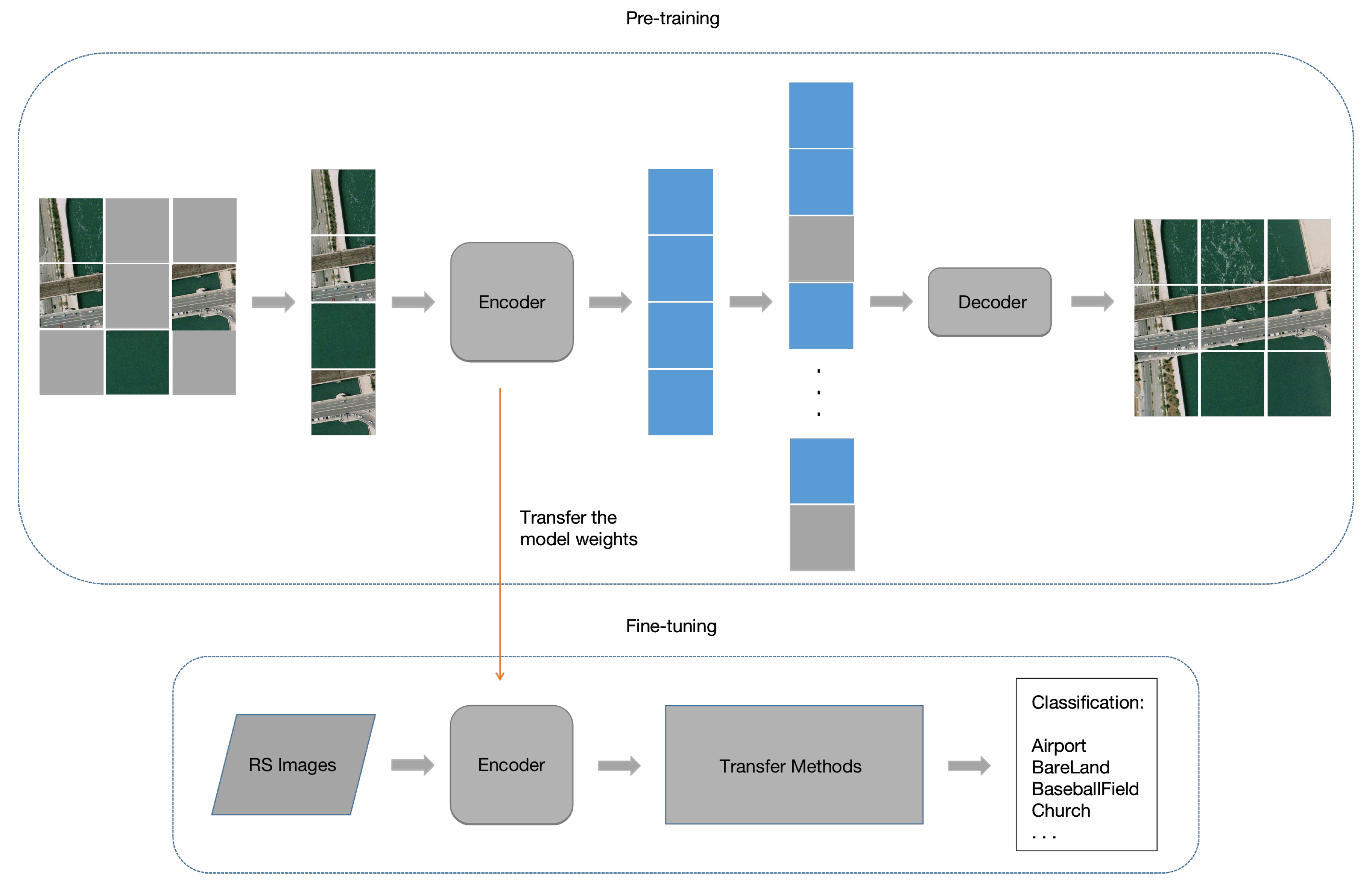
Figure 2 shows our self-supervised learning training process, and the overall architecture of MAE can be seen in the upper part of the figure. Like regular autoencoders, we use an encoder to map the input information to a latent representation, and then we use a decoder to reconstruct the original information using the latent representation. The self-supervised learning training process is divided into two stages: pre-training and fine-tuning. First, representation learning is performed on large-scale unlabeled datasets through pre-training. Then, we use transfer learning to combine self-supervised and remote sensing image classification tasks by fine-tuning a small number of epochs on the labeled dataset. During pre-training, we will use the imagenet-1k [46] dataset, which does not contain labels for training. Additionally, a large number of patches (e.g., 75%) of image patches are randomly masked out. The encoder only performs feature processing on the unmasked part. Mask tokens are introduced after the encoder, and all encoded patch sets and mask tokens are fed into a small decoder for processing, which reconstructs the original image at the pixel level. The masking and reconstruction work on the image can be seen in Figure 3. The pre-trained encoder has a good representation learning ability, corresponding to the weights obtained by the model trained on the unlabeled dataset. Our MIM model uses ViT [15] as the backbone, and the corresponding encoder part consists of alternating layers of Multi-Head Self-Attention (MSA) and multi-layer perceptrons (MLPs) blocks. Layernorm (LN) [47] is applied before each block, and residual connections are applied after each block. If we denote the corresponding number of layers by l and the resulting representation by Z, we can obtain the following representation of the model:
Z l = M S A ( L N ( Z l 1 ) ) + Z l 1
Z l = M L P ( L N ( Z l ) ) + Z l
After pre-training, the decoder is discarded, and we only use the encoder to perform simple fine-tuning on the labeled remote sensing image scene classification dataset, thereby transferring the model weights obtained from unsupervised pre-training to the downstream task of RS image classification.
The MIM model consists of an encoder and a decoder, where the encoder is ViT [15], which handles visible, unmasked patches. We use the settings in ViT to embed patches via linear projection and to add positional embeddings, then we feed the patches into many Transformer blocks to obtain the output. However, the encoder here will remove the mask part and only process the unmask part of each image. Only a small fraction (e.g., 25%)) needs to be processed per image. So, the computation and memory consumption of training the encoder will be small. The input to the decoder consists of encoded visible patches and mask tokens. See Figure 2. Each mask token is a learnable vector representing the missing part to be predicted. All tokens in this complete set have positional embedding information; masked tokens would not be able to find their relative positions without this. The decoder also uses a lot of Transformer modules. Only during pre-training does the decoder participate in the image reconstruction task (replying the mask part with the output of the encoder). The decoder is discarded, and only the encoder is used for fine-tuning on downstream tasks after pre-training.
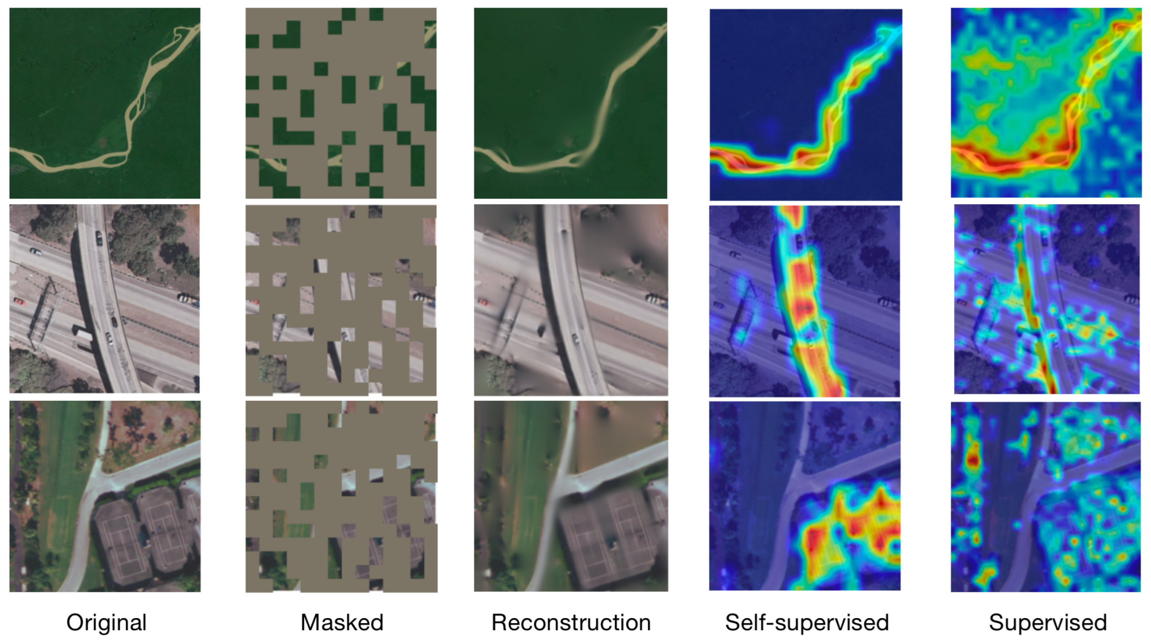
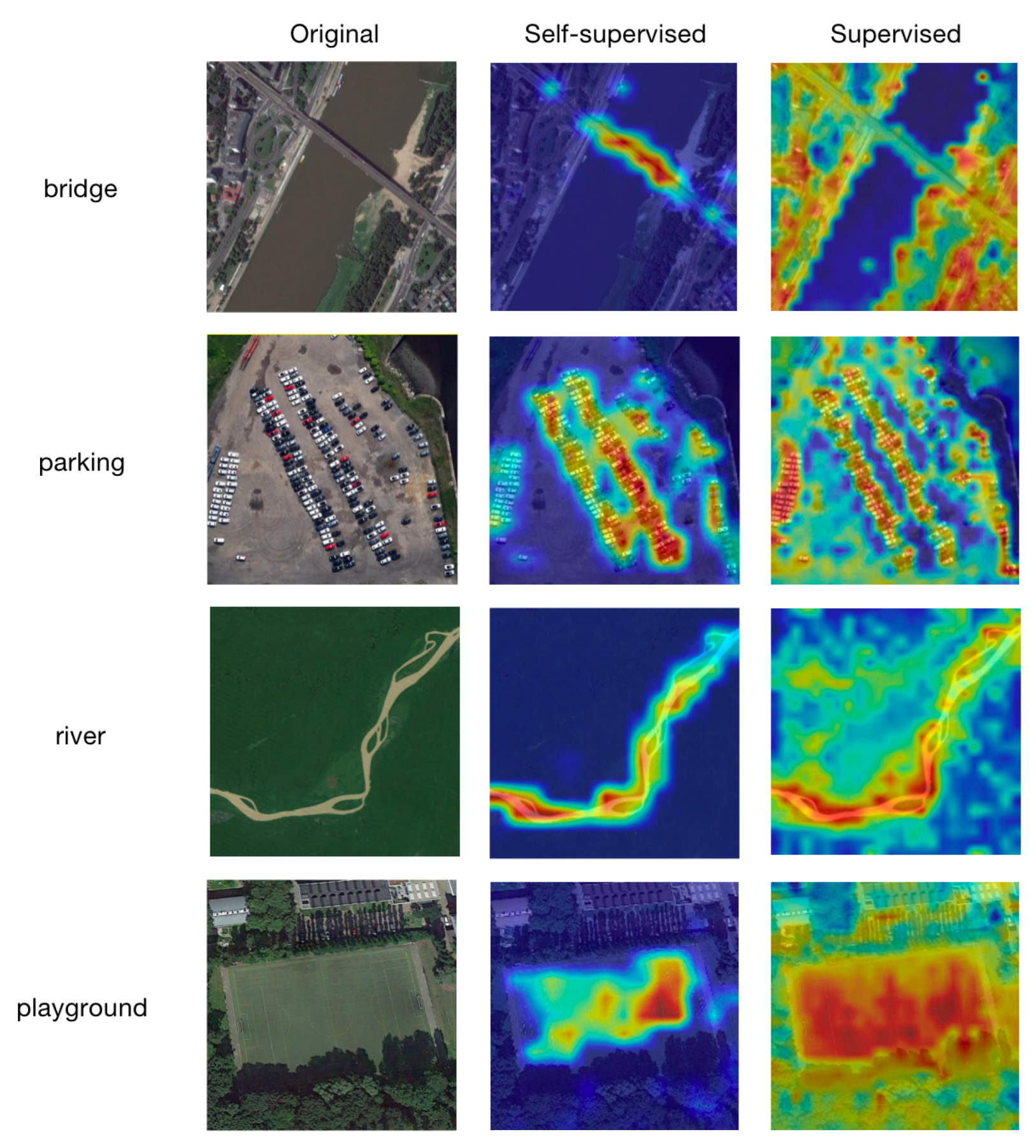
The MIM method uses only a small amount of information to restore the complete picture by masking out most of the redundant information in the picture. Due to the focus on the correlation and continuity of different parts, MIM will be more suitable for the representation learning of a small amount of complex information and transfer to downstream tasks. Especially when there are few target objects in the picture and there is a lot of background information, the MIM method can pay more attention to the object itself. In the subsequent visualization, we can also clearly see that the method focuses on the target object itself and has a clear sense of boundaries.
In this paper, we use the MIM model, using it to perform unlabeled self-supervised learning training results on the imagenet-1k dataset. To further combine self-supervised learning with remote sensing images, we will perform transfer learning for remote sensing image scene classification tasks. In order to study the various effects of self-supervision on remote sensing images, we developed three transfer learning techniques.

3.2. Three Methods for Transfer Learning

By using a large-scale unlabeled dataset and by designing effective pretext tasks, self-supervised learning can theoretically learn a global knowledge representation, but how to ensure that this knowledge representation can be effectively transferred to the target task is not yet conclusive. If a unified feature transfer method is adopted, the transfer may be invalid or even damage the generalization of the model. Another core research question for establishing an effective self-supervised remote sensing interpretation framework is which transfer strategy should be adopted to achieve the best effect. In order to combine MIM-based self-supervised learning and remote sensing image scene classification tasks well, we designed three transfer learning methods to transfer the pre-trained models to downstream tasks. The first two methods need to set hyperparameters and adjust the model: 1. Linear probing [48] (only the last linear layer parameter is updated). 2. End-to-end fine-tuning [48], also known as fine-tuning (update all model parameters). In addition, in order to exclude the influence of hyperparameters on downstream tasks, we also use the method of KNN classification [8] to complete the classification task. Below, we describe these three methods.
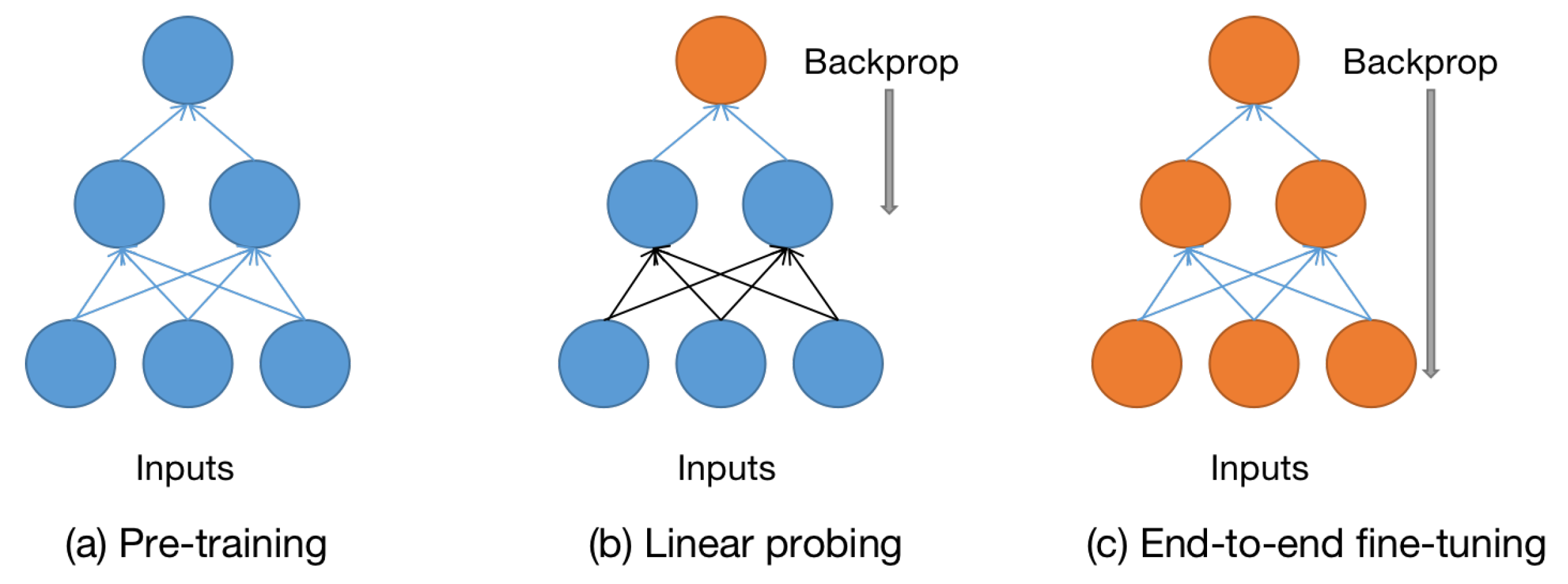
Linear probing and end-to-end fine-tuning are used to optimize the pre-trained model based on the dataset of the downstream task. The principle of fine-tuning is to use the known network structure and known network parameters, modify the corresponding output layer according to the requirements, and fine-tune the parameters of several layers. The difference between these two fine-tuning methods and pre-training methods can be seen from Figure 4. Since the pre-trained model has learned a certain representation ability, fine-tuning does not require the model to be trained from scratch on large-scale data. This is also a good thing for the small-scale remote sensing image scene classification dataset. This method effectively utilizes the powerful generalization ability of deep neural networks, and avoids designing complex models and time-consuming training.
For linear probing, we only update the classifier, keeping the other parameters of the pre-trained model unchanged. As shown in Figure 4, linear probing only updates the linear classifier in the last layer of the model, freezing all previous layers. In general, regularization is not good for linear detection, so we remove many common regularization strategies: we do not use cutmix [49], mixup [50], color jittering, or drop path [51]. We only perform some weak augmentations, such as RandomResizedCrop and RandomHorizontalFlip. We chose LARS [52] as our optimizer when doing linear probing, and the weight decay was set to zero. Normally, when training a linear classifier (e.g., SVM [53]), the normalized input is passed to the classifier. Here, we normalize the pre-trained features and use them to train a linear classifier. Following [28], we use an additional BatchNorm(BN) layer [54] without affine transformation (affine = False). It is beneficial to use BN to normalize the pre-trained features when training the linear probing classifier. We use B to denote a mini-batch of size m for the entire training set, and x to denote its elements. The empirical mean and variance of B could thus be denoted through function (3). The outcome of normalization is x ^ i . Here, ε is an arbitrarily small constant that is added to the denominator to improve numerical stability. Finally, the results of BN can be obtained using two learnable hyperparameters.
μ B = 1 m i = 1 m x i , σ B 2 = 1 m i = 1 m ( x i μ B ) 2
x ^ i = x i μ B σ B 2 + ε
y i = γ x ^ i + β = B N γ , β ( x i )
This layer should be placed before the linear classifier to process the pre-trained features generated by the encoder. We note that one layer does not harm the classification performance, and it can be absorbed into the linear classifier after training: it is better at parameterizing the linear classifier. For linear probing and end-to-end fine-tuning, the classifier uses cross-entropy (CE) loss to calculate the difference between the predicted result and the real result. The expression is then as follows:
c r o s s e n t r o p y = i = 1 n p ( x i ) l n ( q ( x i ) )
where p ( x i ) is the ground truth label and q ( x i ) is the prediction of our model for each input picture. The CE loss function closes the gap between the predicted result and the real result, making the predicted result more like the real result.
For end-to-end fine-tuning, we will train and update all the parameters of the network on the remote sensing dataset. We will compute the gradients of the entire model (rather than just computing the gradients of the final linear classifier as in linear probing), optimize the pre-trained model on the remote sensing scene dataset, and update all network parameters. We will unfreeze the entire pre-trained model and retrain it on remote sensing data with a very low learning rate. By gradually adapting the pre-trained features to new data, the accuracy of the pre-trained model on downstream tasks can be improved. After some fine-tuning after epochs, our model achieves high accuracy. Here, we choose the data augmentation method of RandomAug [55], mixup, and cutmix. Like most Transformer models, we use AdamW [56] as the optimizer. Similar to linear probing, we also normalize the input to the linear classifier. Here, we use the LayerNorm (LN) [47] layer for normalization. LN is an algorithm independent of batch size, so no matter the number of samples, it will not affect the amount of data involved in LN calculation. Let H be the number of hidden layer nodes in a layer, and let l be the number of layers; we can calculate the normalized statistics μ and σ of LN:
μ l = 1 H i = 1 H a i l , σ l = 1 H i = 1 H ( a i l μ l ) 2
The calculation of the statistics here has nothing to do with the number of samples, and it is easier to ensure that the normalized statistics of LN are sufficiently representative. The normalized value a ^ l can be obtained by μ l and σ l . ϵ is a small decimal, preventing division by 0. In LN, we also need a set of parameters called gain g and bias b, to ensure that the normalization operation does not destroy the previous information. Assuming that the activation function is f, the output of the final LN is h l .
a ^ l = a l μ l ( σ l ) 2 + ϵ
h l = f ( g l a ^ l + b l )
Combining the above two formulas and ignoring the parameter l, we have:
h = f ( g σ 2 + ϵ ( a μ ) + b )
Finally, our end-to-end fine-tuning achieves good results on three publicly available remote sensing datasets, surpassing most fully supervised CNN-based models and approaching SOTA’s fully supervised Transformer-based models.
KNN classification directly utilizes the weights obtained via pre-training to directly study the representational ability of self-supervised pre-trained models. The KNN method freezes the entire pre-trained model, and computes and stores the features of the training data for downstream tasks. Regarding the feature selection of the model output, there are generally two kinds—class tokens as global features, and a series of patch tokens composed of each patch. If a patch token is selected, an average pooling operation is required to obtain the final feature result. If a class token is selected, it can be directly used as a global feature for the next calculation. For the classification effect, there is not much difference between the two methods on the classification effect, so for the sake of convenience, we choose the class token for processing. After that, we extract features for each image in the test set and training set, and save the feature results output by the model. For each image in the test set, we multiply its feature matrix with all the training set feature matrices. According to the sorting, we select the k training set images with the smallest difference between their features (here, we set k to 10 according to the scale of the dataset). For the k images in the training set, we count their class labels and use the class with the most occurrences as the new label for this test set image. Finally, we calculate the accuracy of the entire dataset based on the inference results of each test set image. The KNN classification method does not require any other hyperparameter tuning or data augmentation, and can be run only with downstream datasets, which greatly simplifies the transfer of pre-trained models to downstream tasks.

4. Experiments and Results

4.1. Dataset Description

We test our method on three publicly available remote sensing image datasets, named NWPU-RESISC45 dataset (NWPU) [57], Aerial Image dataset (AID) [58], and UCMerced Land-Use dataset (UCM) [59]. Table 1 shows the specific details of these three datasets.

4.2. Training Details

The training equipment that we used is shown in Table 2. All experiments are trained for 120 epochs. All experiments were implemented using Pytoch 1.8.1. The models were trained on a Tesla P40 (24 GB) GPU × 4 in a single machine. We used the MAE model to study our self-supervised MIM strategy, and used ViT-B [15] as the backbone of our model. When ViT processes pictures, it will divide a picture into multiple patches. Here, we set the patch size to 16 × 16. For the AID dataset, and the NWPU, and UCM datasets, we reshaped the images to 224 × 224 pixels in order to reduce content loss. We set the batch size to 64, and since four GPUS were used, the total batch size was 256. We used 12 Transformer encoders, and the final class head is a simple linear layer that outputs classification results.
Since self-supervised pre-training requires more computing power, we will use pre-trained weights obtained via unlabeled self-supervised training of the MIM model on imagenet-1k. We fine-tune the pre-trained model and conduct studies on three different transfer methods to explore how well self-supervised learning works on downstream tasks. For fine-tuning, we use AdamW as the optimizer. The learning rate is set to 0.001, and the weight decay is set to 0.05. For linear probing, we use LARS [52] as the optimizer. The learning rate is set to 0.1, and the weight decay is set to 0. For KNN, we set the KNN number to 10; that is, we select the 10 training set images that are closest to the test image features for voting, and obtain the new label of the image. When performing the two downstream tasks of fine-tuning and KNN, we use the mmselfsup open source model. The training code will be available at: https://github.com/open-mmlab/mmselfsup, accessed on 15 June 2022. For linear probing, we are using the Meta open source model. The training code will be available at: https://github.com/facebookresearch/MAE, accessed on 15 June 2022.
For each dataset, we randomly select a portion of the dataset as the training set, and the rest as the test set. For NWPU, we set the training set ratio to 10% and 20%. For AID, we set the training set proportions to 20% and 50%. For UC-Merced, we set the training set proportions to 50% and 80%. In addition, common evaluation metrics for scene classification include overall accuracy (OA) and confusion matrix (CM). In addition, since our dataset is divided into training and test sets via random sampling, all experiments are repeated 10 times to reduce random effects. The experimental results represent the mean overall accuracy as a standard deviation (OA ± STD).

4.3. Comparison of Three Transfer Methods

To validate the effectiveness of our self-supervised learning approach on downstream tasks, we conducted three experiments on the three datasets. Table 3 presents the results of the experiments of models under three different transfer methods.
As can be seen from the table, the accuracy obtained via end-to-end fine-tuning is more than 90%, but the linear probing is between 70% and 90%, and KNN is between 60% and 90%. Fine-tuning can achieve better classification results than KNN and linear probing. It can be seen from the comparison of different datasets that for larger-scale datasets, such as the NWPU and AID datasets, that end-to-end fine-tuning can achieve better results than the other two methods. For smaller-scale datasets, such as UCM, all three methods can achieve better results, and the gap is small.
Overall, it can be seen from the above results that linear probing outperforms the KNN method, and that end-to-end fine-tuning outperforms linear probing. When the dataset is large and complex, end-to-end fine-tuning is much better than the other two methods. This shows that in this case, more sufficient update parameters are needed for transfer learning in order to fully combine self-supervision and remote sensing scenes. When the dataset is relatively simple, linear probing can achieve good results with less training time and a simpler parameter update method—which also makes it possible to quickly implement transfer learning with limited computing power. For the KNN method that does not require hyperparameters and parameter updates at all, the MIM self-supervised learning method can also achieve a classification effect with an accuracy of greater than 80% in a simple dataset scenario. KNN embodies the potential of self-supervised representation learning from the side. These three methods show how reliable and useful our self-supervised learning approach is. They also show how important fine-tuning is.

4.4. Self-Supervised Visualization

As shown in Figure 5, we show the visualization of AID. The left column represents the original image of the remote sensing scene classification dataset, the middle column represents the visualization obtained by the self-supervised model, and the right column represents the visualization obtained by the fully supervised model. Since our self-supervised model backbone is ViT-B [15], ViT-B is also selected as the comparison object for full supervision. We use the grad-cam method for visualization, and gradients for visualization. The final classification is performed on the class labels computed in the last attention block, the output is the category at the end, and the gradient corresponding to the output is 0, so we should choose any layer before the final attention block. Here, we select the norm layer of the last Transformer module of the ViT-backbone, which is before the last fully connected layer.
For the AID dataset, we can clearly see the “river” in Figure 5; the self-supervised attention is all on the river itself, and the visual attention map has a good sense of boundaries. Although the full supervisor also paid attention to the river itself; it scatters a lot of attention to the parts unrelated to the river, which shows that the essential characteristics of “river” are not well grasped, and that it is easily imaged by other objects. For most remote sensing images, the self-supervised attention part mainly focuses on the key parts and tends to focus on complete and specific scene objects, and the visual attention map is very concentrated and has a good sense of boundaries. The attention part of the full supervision is all over the whole map, the attention is relatively scattered, and sometimes it pays attention to the non-critical parts, and cannot pay attention to the key parts.

4.5. Comparison with Previous Results

The main goal of this paper is to demonstrate that self-supervised learning can improve the performance of networks. Therefore, we use three types of methods to compare our proposed approach with other state-of-the-art baselines. For remote sensing scene classification, we will select the best results of the self-supervised downstream task fine-tuning and compare them with CNN-based models, Transformer-based models, and some self-supervised methods. The evaluation metric is the overall classification accuracy (OA). In addition, we use the training results obtained by using a larger training set split ratio for each dataset to draw a confusion matrix to show the classification of each category.
(1) Comparison with CNN-based models: As shown in Table 4, Table 5 and Table 6, on the NWPU dataset, the overall accuracies of our self-supervised method are 91.98% and 94.48% with training ratios of 10% and 20%, respectively. On the AID dataset, the overall accuracies of our self-supervised method are 95.71% and 97.65% with training ratios of 20% and 50%, respectively. On the UCM dataset, the overall accuracies of our self-supervised method are 97.86% and 99.24% with training ratios of 50% and 80%, respectively. Our self-supervised method outperforms almost all of the CNN-based methods with simple fine-tuning, using only the pre-trained weights from the unlabeled training set, and performs well with different training proportions on the three datasets.
On the NWPU dataset, at 20% training scale, Figure 6 shows the confusion matrix generated by the classification results obtained by our self-supervised method. As you can see from the confusion matrix, the accuracy rate for most classes is greater than 95%. We observed the greatest confusion between the “palace” and “church” categories. The main reason may be that these two classes have high inter-class similarity.
(2) Comparison with Transformer-based models: We also compared our self-supervised approach with other Transformers. Experimental results are shown in Table 7. Our self-supervised method is close to the Transformer state-of-the-art model.
The experimental results show that directly using global attention-based ViT [15] performs mediocrely in remote sensing scene classification, but ViT-Hybrid [15] performs well. The Swin Transformer uses windows to combine local and global attention information, and the results show that it far outperforms CNN-based methods. TRS [74] also has good results using the Transformer model, which is the current SOTA model. However, our self-supervised approach, with label-free pre-trained weights and simple fine-tuning, achieves good results. On the AID dataset, at a 20% training rate, our method is the most effective, outperforming the TRS model by 0.17%.
(3) Comparison with other self-supervised models: There are few studies on self-supervised learning applied to remote sensing scene classification, and we need to conduct more exploration and research. We found two self-supervised methods, ResNet-101+MTL and ResNeXt-101+MTL [72], for remote sensing scene classification to compare with our method. The experimental results are shown in Table 8.
Our method outperforms the original method on all experiments of the three datasets. Among them, ResNeXt-101+MTL is better than ResNet-101+MTL. On the NWPU dataset, at a 20% training rate, our method outperforms ResNeXt-101+MTL by 0.27%. On the AID dataset, at a 20% training rate, our method outperforms ResNeXt-101+MTL by 1.75%. On the UCM dataset, at a 80% training rate, our method outperforms ResNeXt-101+MTL by 0.13%.

5. Discussion

Self-supervised learning is not only able to benefit from massive unlabeled data-driven model learning at low cost, but it can also make full use of pretext tasks to mine the rich inherent information of image data, resulting in improved performance in remote sensing image intelligence tasks. How to utilize the inherent relationship between self-supervised learning and remote sensing image representation, as well as how to effectively transfer self-supervised learning characteristics, are crucial issues in the research on the intelligent interpretation of remote sensing images under conditions of extremely abundant data sources. To this end, we conducted a series of studies combining MIM self-supervised learning with remote sensing image scene classification for the first time.
In this study, we mainly focused on three aspects: (1) For the first time, MIM self-supervised learning is studied on the traditional remote sensing image scene classification task, and the unlabeled dataset is used for representation learning to better learn remote sensing. (2) In order to better combine self-supervised learning with remote sensing scene classification, we designed three different transfer learning methods to study the transfer effect of self-supervised learning on remote sensing image scene classification from different perspectives. (3) To reveal how self-supervision achieves better representation, we conduct a visual study of model-specific feature layers and compare them with fully supervised models. Our work provides reliable guidance for self-supervised analysis on remote sensing images. In the future, we will investigate not only classification tasks, but also the segmentation and detection of remote sensing images, using our self-supervised method.

6. Conclusions

In this paper, we investigate MIM self-supervised learning in the task of remote sensing image scene classification for the first time. Using the MIM strategy, pre-training on unlabeled datasets, and then simply fine-tuning on labeled remote sensing datasets without the use of other supervised strategies, we achieve good classification results. Concurrently, in order to improve the combination of self-supervised and remote sensing images, we developed three distinct methods for transfer learning to apply the self-supervised learning representations to the classic downstream task of remote sensing image classification. Finally, we perform a visual analysis of the feature network layer, and the results demonstrate that self-supervised learning has a better representation learning effect than fully supervised learning, and it focuses more precise and concentrated attention on the target subject, which has a good representation learning potential. The results of the experiment show that our self-supervised method works well on public datasets and does better than most fully supervised learning methods without using other supervised remote sensing image analysis strategies.

Author Contributions

Conceptualization, Y.G.; methodology, Y.G.; software, Y.G.; validation, Y.G.; formal analysis, Y.G.; investigation, Y.G.; resources, Y.G.; data curation, Y.G.; writing—original draft preparation, Y.G.; writing—review and editing, Y.G., X.S. and C.L.; visualization, Y.G.; supervision, C.L. and X.S.; project administration, C.L. All authors have read and agreed to the published version of the manuscript.

Funding

This research received no external funding.

Data Availability Statement

Data sharing is not applicable to this article.

Acknowledgments

The authors thank the reviewers for their valuable suggestions and comments. We also thank the production team for formatting the manuscript.

Conflicts of Interest

The author declares no conflict of interest.

References

  1. Hu, Q.; Wu, W.; Xia, T.; Yu, Q.; Yang, P.; Li, Z.; Song, Q. Exploring the use of Google Earth imagery and object-based methods in land use/cover mapping. Remote Sens. 2013, 5, 6026–6042. [Google Scholar] [CrossRef]
  2. Zheng, X.; Gong, T.; Li, X.; Lu, X. Generalized scene classification from small-scale datasets with multitask learning. IEEE Trans. Geosci. Remote Sens. 2021, 60, 1–11. [Google Scholar] [CrossRef]
  3. Toth, C.; Jóźków, G. Remote sensing platforms and sensors: A survey. ISPRS J. Photogramm. Remote Sens. 2016, 115, 22–36. [Google Scholar] [CrossRef]
  4. Zheng, X.; Wang, B.; Du, X.; Lu, X. Mutual attention inception network for remote sensing visual question answering. IEEE Trans. Geosci. Remote Sens. 2021, 60, 1–14. [Google Scholar] [CrossRef]
  5. Li, K.; Wan, G.; Cheng, G.; Meng, L.; Han, J. Object detection in optical remote sensing images: A survey and a new benchmark. ISPRS J. Photogramm. Remote Sens. 2020, 159, 296–307. [Google Scholar] [CrossRef]
  6. Chen, M.; Liu, D.; Qian, K.; Li, J.; Lei, M.; Zhou, Y. Lunar crater detection based on terrain analysis and mathematical morphology methods using digital elevation models. IEEE Trans. Geosci. Remote Sens. 2018, 56, 3681–3692. [Google Scholar] [CrossRef]
  7. Ye, F.; Xiao, H.; Zhao, X.; Dong, M.; Luo, W.; Min, W. Remote sensing image retrieval using convolutional neural network features and weighted distance. IEEE Geosci. Remote Sens. Lett. 2018, 15, 1535–1539. [Google Scholar] [CrossRef]
  8. Guo, G.; Wang, H.; Bell, D.; Bi, Y.; Greer, K. KNN model-based approach in classification. In Proceedings of the OTM Confederated International Conferences on the Move to Meaningful Internet Systems, Sicily, Italy, 3–7 November 2003; Springer: Berlin/Heidelberg, Germany, 2003; pp. 986–996. [Google Scholar]
  9. Wu, Z.; Xiong, Y.; Yu, S.X.; Lin, D. Unsupervised feature learning via non-parametric instance discrimination. In Proceedings of the IEEE Conference on Computer Vision and Pattern Recognition, Salt Lake City, UT, USA, 18–23 June 2018; pp. 3733–3742. [Google Scholar]
  10. Vaswani, A.; Shazeer, N.; Parmar, N.; Uszkoreit, J.; Jones, L.; Gomez, A.N.; Kaiser, Ł.; Polosukhin, I. Attention is all you need. Adv. Neural Inf. Process. Syst. 2017, 30. [Google Scholar] [CrossRef]
  11. Cho, K.; Van Merriënboer, B.; Gulcehre, C.; Bahdanau, D.; Bougares, F.; Schwenk, H.; Bengio, Y. Learning phrase representations using RNN encoder-decoder for statistical machine translation. arXiv 2014, arXiv:1406.1078. [Google Scholar]
  12. Stewart, R.; Andriluka, M.; Ng, A.Y. End-to-end people detection in crowded scenes. In Proceedings of the IEEE Conference on Computer Vision and Pattern Recognition, Las Vegas, NV, USA, 27–30 June 2016; pp. 2325–2333. [Google Scholar]
  13. Parmar, N.; Vaswani, A.; Uszkoreit, J.; Kaiser, L.; Shazeer, N.; Ku, A.; Tran, D. Image transformer. In Proceedings of the International Conference on Machine Learning, Stockholm, Sweden, 10–15 July 2018; pp. 4055–4064. [Google Scholar]
  14. Child, R.; Gray, S.; Radford, A.; Sutskever, I. Generating long sequences with sparse transformers. arXiv 2019, arXiv:1904.10509. [Google Scholar]
  15. Dosovitskiy, A.; Beyer, L.; Kolesnikov, A.; Weissenborn, D.; Zhai, X.; Unterthiner, T.; Dehghani, M.; Minderer, M.; Heigold, G.; Gelly, S.; et al. An image is worth 16x16 words: Transformers for image recognition at scale. arXiv 2020, arXiv:2010.11929. [Google Scholar]
  16. Bello, I.; Zoph, B.; Vaswani, A.; Shlens, J.; Le, Q.V. Attention augmented convolutional networks. In Proceedings of the IEEE/CVF International Conference on Computer Vision, Seoul, Korea, 27 October–2 November 2019; pp. 3286–3295. [Google Scholar]
  17. Carion, N.; Massa, F.; Synnaeve, G.; Usunier, N.; Kirillov, A.; Zagoruyko, S. End-to-end object detection with transformers. In Proceedings of the European Conference on Computer Vision, Glasgow, UK, 23–28 August 2020; Springer: Cham, Switzerland, 2020; pp. 213–229. [Google Scholar]
  18. Touvron, H.; Cord, M.; Douze, M.; Massa, F.; Sablayrolles, A.; Jégou, H. Training data-efficient image transformers & distillation through attention. In Proceedings of the International Conference on Machine Learning, Virtual, 18–24 July 2021; pp. 10347–10357. [Google Scholar]
  19. Yuan, L.; Chen, Y.; Wang, T.; Yu, W.; Shi, Y.; Jiang, Z.H.; Tay, F.E.; Feng, J.; Yan, S. Tokens-to-token vit: Training vision transformers from scratch on imagenet. In Proceedings of the IEEE/CVF International Conference on Computer Vision, Montreal, QC, Canada, 10–17 October 2021; pp. 558–567. [Google Scholar]
  20. Abnar, S.; Dehghani, M.; Zuidema, W. Transferring inductive biases through knowledge distillation. arXiv 2020, arXiv:2006.00555. [Google Scholar]
  21. Li, W.; Cao, D.; Peng, Y.; Yang, C. MSNet: A multi-stream fusion network for remote sensing spatiotemporal fusion based on transformer and convolution. Remote Sens. 2021, 13, 3724. [Google Scholar] [CrossRef]
  22. Bazi, Y.; Bashmal, L.; Rahhal, M.M.A.; Dayil, R.A.; Ajlan, N.A. Vision transformers for remote sensing image classification. Remote Sens. 2021, 13, 516. [Google Scholar] [CrossRef]
  23. Xu, Z.; Zhang, W.; Zhang, T.; Yang, Z.; Li, J. Efficient transformer for remote sensing image segmentation. Remote Sens. 2021, 13, 3585. [Google Scholar] [CrossRef]
  24. Devlin, J.; Chang, M.W.; Lee, K.; Toutanova, K. Bert: Pre-training of deep bidirectional transformers for language understanding. arXiv 2018, arXiv:1810.04805. [Google Scholar]
  25. Liu, Y.; Ott, M.; Goyal, N.; Du, J.; Joshi, M.; Chen, D.; Levy, O.; Lewis, M.; Zettlemoyer, L.; Stoyanov, V. Roberta: A robustly optimized bert pretraining approach. arXiv 2019, arXiv:1907.11692. [Google Scholar]
  26. Brown, T.; Mann, B.; Ryder, N.; Subbiah, M.; Kaplan, J.D.; Dhariwal, P.; Neelakantan, A.; Shyam, P.; Sastry, G.; Askell, A.; et al. Language models are few-shot learners. Adv. Neural Inf. Process. Syst. 2020, 33, 1877–1901. [Google Scholar]
  27. Chen, M.; Radford, A.; Child, R.; Wu, J.; Jun, H.; Dhariwal, P.; Luan, D.; Sutskever, I. Generative pretraining from pixels. In Proceedings of the 37th International Conference on Machine Learning, Virtual, 13–18 July 2020; Volume 1, p. 1. [Google Scholar]
  28. Doersch, C.; Gupta, A.; Efros, A.A. Unsupervised visual representation learning by context prediction. In Proceedings of the IEEE International Conference on Computer Vision, Santiago, Chile, 7–13 December 2015; pp. 1422–1430. [Google Scholar]
  29. Yang, C.; Xu, Y.; Dai, B.; Zhou, B. Video representation learning with visual tempo consistency. arXiv 2020, arXiv:2006.15489. [Google Scholar]
  30. Pathak, D.; Krahenbuhl, P.; Donahue, J.; Darrell, T.; Efros, A.A. Context encoders: Feature learning by inpainting. In Proceedings of the IEEE Conference on Computer Vision and Pattern Recognition, Las Vegas, NV, USA, 27–30 June 2016; pp. 2536–2544. [Google Scholar]
  31. Hinton, G.E.; Zemel, R. Autoencoders, minimum description length and Helmholtz free energy. Adv. Neural Inf. Process. Syst. 1993, 6, 3–10. [Google Scholar]
  32. Vincent, P.; Larochelle, H.; Bengio, Y.; Manzagol, P.A. Extracting and composing robust features with denoising autoencoders. In Proceedings of the 25th International Conference on Machine Learning, Helsinki, Finland, 5–9 July 2008; pp. 1096–1103. [Google Scholar]
  33. He, K.; Chen, X.; Xie, S.; Li, Y.; Dollár, P.; Girshick, R. Masked autoencoders are scalable vision learners. In Proceedings of the IEEE/CVF Conference on Computer Vision and Pattern Recognition, London, UK, 21–23 June 2022; pp. 16000–16009. [Google Scholar]
  34. Xie, Z.; Zhang, Z.; Cao, Y.; Lin, Y.; Bao, J.; Yao, Z.; Dai, Q.; Hu, H. Simmim: A simple framework for masked image modeling. In Proceedings of the IEEE/CVF Conference on Computer Vision and Pattern Recognition, New Orleans, LA, USA, 19–23 June 2022; pp. 9653–9663. [Google Scholar]
  35. Zhai, X.; Oliver, A.; Kolesnikov, A.; Beyer, L. S4l: Self-supervised semi-supervised learning. In Proceedings of the IEEE/CVF International Conference on Computer Vision, Seoul, Korea, 27 October–2 November 2019; pp. 1476–1485. [Google Scholar]
  36. Doersch, C.; Zisserman, A. Multi-task self-supervised visual learning. In Proceedings of the IEEE International Conference on Computer Vision, Venice, Italy, 22–29 October 2017; pp. 2051–2060. [Google Scholar]
  37. Sinaga, K.P.; Yang, M.S. Unsupervised K-means clustering algorithm. IEEE Access 2020, 8, 80716–80727. [Google Scholar] [CrossRef]
  38. Gidaris, S.; Singh, P.; Komodakis, N. Unsupervised representation learning by predicting image rotations. arXiv 2018, arXiv:1803.07728. [Google Scholar]
  39. Noroozi, M.; Vinjimoor, A.; Favaro, P.; Pirsiavash, H. Boosting self-supervised learning via knowledge transfer. In Proceedings of the IEEE Conference on Computer Vision and Pattern Recognition, Salt Lake City, UT, USA, 18–23 June 2018; pp. 9359–9367. [Google Scholar]
  40. Noroozi, M.; Favaro, P. Unsupervised learning of visual representations by solving jigsaw puzzles. In Proceedings of the European Conference on Computer Vision, Amsterdam, The Netherlands, 11–14 October 2016; Springer: Cham, Switzerland, 2016; pp. 69–84. [Google Scholar]
  41. Becker, S.; Hinton, G.E. Self-organizing neural network that discovers surfaces in random-dot stereograms. Nature 1992, 355, 161–163. [Google Scholar] [CrossRef]
  42. Hadsell, R.; Chopra, S.; LeCun, Y. Dimensionality reduction by learning an invariant mapping. In Proceedings of the 2006 IEEE Computer Society Conference on Computer Vision and Pattern Recognition (CVPR’06), New York, NY, USA, 17–22 June 2006; Volume 2, pp. 1735–1742. [Google Scholar]
  43. He, K.; Fan, H.; Wu, Y.; Xie, S.; Girshick, R. Momentum contrast for unsupervised visual representation learning. In Proceedings of the IEEE/CVF Conference on Computer Vision and Pattern Recognition, Seattle, WA, USA, 13–19 June 2020; pp. 9729–9738. [Google Scholar]
  44. Chen, T.; Kornblith, S.; Norouzi, M.; Hinton, G. A simple framework for contrastive learning of visual representations. In Proceedings of the International Conference on Machine Learning, Virtual, 13–18 July 2020; pp. 1597–1607. [Google Scholar]
  45. Bao, H.; Dong, L.; Wei, F. Beit: Bert pre-training of image transformers. arXiv 2021, arXiv:2106.08254. [Google Scholar]
  46. Krizhevsky, A.; Sutskever, I.; Hinton, G.E. Imagenet classification with deep convolutional neural networks. Commun. ACM 2017, 60, 84–90. [Google Scholar] [CrossRef]
  47. Ba, J.L.; Kiros, J.R.; Hinton, G.E. Layer normalization. arXiv 2016, arXiv:1607.06450. [Google Scholar]
  48. Wang, C.; Wu, Y.; Liu, S.; Yang, Z.; Zhou, M. Bridging the gap between pre-training and fine-tuning for end-to-end speech translation. In Proceedings of the AAAI Conference on Artificial Intelligence, New York, NY, USA, 7–12 February 2020; Volume 34, pp. 9161–9168. [Google Scholar]
  49. Yun, S.; Han, D.; Oh, S.J.; Chun, S.; Choe, J.; Yoo, Y. Cutmix: Regularization strategy to train strong classifiers with localizable features. In Proceedings of the IEEE/CVF International Conference on Computer Vision, Seoul, Korea, 27 October–2 November 2019; pp. 6023–6032. [Google Scholar]
  50. Zhang, H.; Cisse, M.; Dauphin, Y.N.; Lopez-Paz, D. mixup: Beyond empirical risk minimization. arXiv 2017, arXiv:1710.09412. [Google Scholar]
  51. Huang, G.; Sun, Y.; Liu, Z.; Sedra, D.; Weinberger, K.Q. Deep networks with stochastic depth. In Proceedings of the European Conference on Computer Vision, Amsterdam, The Netherlands, 11–14 October 2016; Springer: Cham, Switzerland, 2016; pp. 646–661. [Google Scholar]
  52. You, Y.; Gitman, I.; Ginsburg, B. Large batch training of convolutional networks. arXiv 2017, arXiv:1708.03888. [Google Scholar]
  53. Cortes, C.; Vapnik, V. Support-vector networks. Mach. Learn. 1995, 20, 273–297. [Google Scholar] [CrossRef]
  54. Ioffe, S.; Szegedy, C. Batch normalization: Accelerating deep network training by reducing internal covariate shift. In Proceedings of the International Conference on Machine Learning, Lille, France, 7–9 July 2015; pp. 448–456. [Google Scholar]
  55. Cubuk, E.D.; Zoph, B.; Shlens, J.; Le, Q.V. Randaugment: Practical automated data augmentation with a reduced search space. In Proceedings of the IEEE/CVF Conference on Computer Vision and Pattern Recognition Workshops, Seattle, WA, USA, 14–19 June 2020; pp. 702–703. [Google Scholar]
  56. Ilya, L.; Frank, H. Decoupled weight decay regularization. In Proceedings of the ICLR, New Orleans, LA, USA, 6–9 May 2019. [Google Scholar]
  57. Cheng, G.; Han, J.; Lu, X. Remote sensing image scene classification: Benchmark and state of the art. Proc. IEEE 2017, 105, 1865–1883. [Google Scholar] [CrossRef]
  58. Xia, G.S.; Hu, J.; Hu, F.; Shi, B.; Bai, X.; Zhong, Y.; Zhang, L.; Lu, X. AID: A benchmark data set for performance evaluation of aerial scene classification. IEEE Trans. Geosci. Remote Sens. 2017, 55, 3965–3981. [Google Scholar] [CrossRef]
  59. Zou, Q.; Ni, L.; Zhang, T.; Wang, Q. Deep learning based feature selection for remote sensing scene classification. IEEE Geosci. Remote Sens. Lett. 2015, 12, 2321–2325. [Google Scholar] [CrossRef]
  60. Simonyan, K.; Zisserman, A. Very deep convolutional networks for large-scale image recognition. arXiv 2014, arXiv:1409.1556. [Google Scholar]
  61. Aral, R.A.; Keskin, Ş.R.; Kaya, M.; Hacıömeroğlu, M. Classification of trashnet dataset based on deep learning models. In Proceedings of the 2018 IEEE International Conference on Big Data (Big Data), Seattle, WA, USA, 10–13 December 2018; pp. 2058–2062. [Google Scholar]
  62. Bazi, Y.; Al Rahhal, M.M.; Alhichri, H.; Alajlan, N. Simple yet effective fine-tuning of deep CNNs using an auxiliary classification loss for remote sensing scene classification. Remote Sens. 2019, 11, 2908. [Google Scholar] [CrossRef]
  63. Liu, M.; Jiao, L.; Liu, X.; Li, L.; Liu, F.; Yang, S. C-CNN: Contourlet convolutional neural networks. IEEE Trans. Neural Netw. Learn. Syst. 2020, 32, 2636–2649. [Google Scholar] [CrossRef] [PubMed]
  64. Bi, Q.; Zhang, H.; Qin, K. Multi-scale stacking attention pooling for remote sensing scene classification. Neurocomputing 2021, 436, 147–161. [Google Scholar] [CrossRef]
  65. Zhang, W.; Tang, P.; Zhao, L. Remote sensing image scene classification using CNN-CapsNet. Remote Sens. 2019, 11, 494. [Google Scholar] [CrossRef]
  66. Tang, X.; Ma, Q.; Zhang, X.; Liu, F.; Ma, J.; Jiao, L. Attention consistent network for remote sensing scene classification. IEEE J. Sel. Top. Appl. Earth Obs. Remote Sens. 2021, 14, 2030–2045. [Google Scholar] [CrossRef]
  67. Xu, C.; Zhu, G.; Shu, J. A lightweight and robust lie group-convolutional neural networks joint representation for remote sensing scene classification. IEEE Trans. Geosci. Remote Sens. 2021, 60, 1–15. [Google Scholar] [CrossRef]
  68. Wang, Q.; Liu, S.; Chanussot, J.; Li, X. Scene classification with recurrent attention of VHR remote sensing images. IEEE Trans. Geosci. Remote Sens. 2018, 57, 1155–1167. [Google Scholar] [CrossRef]
  69. Sun, H.; Li, S.; Zheng, X.; Lu, X. Remote sensing scene classification by gated bidirectional network. IEEE Trans. Geosci. Remote Sens. 2019, 58, 82–96. [Google Scholar] [CrossRef]
  70. Zhang, B.; Zhang, Y.; Wang, S. A lightweight and discriminative model for remote sensing scene classification with multidilation pooling module. IEEE J. Sel. Top. Appl. Earth Obs. Remote Sens. 2019, 12, 2636–2653. [Google Scholar] [CrossRef]
  71. Bi, Q.; Qin, K.; Zhang, H.; Xie, J.; Li, Z.; Xu, K. APDC-Net: Attention pooling-based convolutional network for aerial scene classification. IEEE Geosci. Remote Sens. Lett. 2019, 17, 1603–1607. [Google Scholar] [CrossRef]
  72. Zhao, Z.; Luo, Z.; Li, J.; Chen, C.; Piao, Y. When self-supervised learning meets scene classification: Remote sensing scene classification based on a multitask learning framework. Remote Sens. 2020, 12, 3276. [Google Scholar] [CrossRef]
  73. Wang, X.; Wang, S.; Ning, C.; Zhou, H. Enhanced feature pyramid network with deep semantic embedding for remote sensing scene classification. IEEE Trans. Geosci. Remote Sens. 2021, 59, 7918–7932. [Google Scholar] [CrossRef]
  74. Zhang, J.; Zhao, H.; Li, J. TRS: Transformers for remote sensing scene classification. Remote Sens. 2021, 13, 4143. [Google Scholar] [CrossRef]
  75. Wang, W.; Xie, E.; Li, X.; Fan, D.P.; Song, K.; Liang, D.; Lu, T.; Luo, P.; Shao, L. Pyramid vision transformer: A versatile backbone for dense prediction without convolutions. In Proceedings of the IEEE/CVF International Conference on Computer Vision, Virtual, 11–17 October 2021; pp. 568–578. [Google Scholar]
  76. Liu, Z.; Lin, Y.; Cao, Y.; Hu, H.; Wei, Y.; Zhang, Z.; Lin, S.; Guo, B. Swin transformer: Hierarchical vision transformer using shifted windows. In Proceedings of the IEEE/CVF International Conference on Computer Vision, Virtual, 11–17 October 2021; pp. 10012–10022. [Google Scholar]
Figure 1. Some remote sensing images. The categories for each row, from top to bottom, are “river”, “overpass”, and “tennis court.” The images of each category have been processed multiple times, and each row from left to right represents the original image, the image after the mask operation, the image reconstructed using the MIM method, the visualization of self-supervised classification results, and the visualization of fully supervised classification results.
Remotesensing 14 04824 g001
Figure 2. Our self-supervised learning training process.
Remotesensing 14 04824 g002
Figure 3. Reconstruction of masked images via self-supervised learning. Every four images is a group. (Left) Original image. (Middle) Random sampling for mask. (Right) Self-supervised model to reconstruct the image.
Remotesensing 14 04824 g003
Figure 4. Gradient calculation and parameter update under different methods of self-supervised learning: (a) pre-training on unlabeled dataset; (b) linear probing; (c) end-to-end fine-tuning.
Remotesensing 14 04824 g004
Figure 5. Self-supervised and fully supervised learning visualizations on AID datasets.
Remotesensing 14 04824 g005
Figure 6. Confusion matrix for NWPU dataset under 20% training ratio.
Remotesensing 14 04824 g006
Table 1. Characteristic of the datasets.
DatasetScene ClassesImage SizeImages per ClassTotal
NWPU45256 × 25670031,500
AID30600 × 600220∼42010,000
UCM21256 × 2561002100
Table 2. Experimental environment.
Operation SystemUbuntu 16.04.6 LTS
FrameworkPyTorch 1.8.1
Memory251 GB
CPUIntel(R )Xeon(R) E5-2630 v4 @ 2.20 GHz
GPU4 x Tesla P40
Table 3. Classification accuracy of three different transfer methods on three datasets.
DatasetTrain RatioLinear ProbingKNNEnd-to-End Fine-Tuning
NWPU10%70.2962.2391.98
NWPU20%76.9468.0594.48
UCM50%84.4880.3897.86
UCM80%92.8688.3399.24
AID20%80.3474.1095.71
AID50%88.3881.1697.65
Table 4. Classification accuracy on the NWPU dataset compared to CNN-based models (OA ± STD).
MethodTraining Proportion
10%20%
AlexNet [46]76.69 ± 0.1976.85 ± 0.18
VGGNet [60]76.47 ± 0.1879.79 ± 0.65
GoogleNet [58]76.19 ± 0.3878.48 ± 0.26
SPPNet [58]82.13 ± 0.3084.64 ± 0.23
D-CNN with AlexNet [58]85.56 ± 0.2087.24 ± 0.12
D-CNN with VGGNet-16 [58]89.22 ± 0.5091.89 ± 0.22
DenseNet-121 [61]88.31 ± 0.3590.47 ± 0.33
EfficientNet-B0-aux [62]89.96 ± 0.27-
EfficientNet-B3-aux [62]91.08 ± 0.14-
Contourlet CNN [63]85.93 ± 0.5189.57 ± 0.45
VGG-MS2AP [64]92.27 ± 0.2193.91 ± 0.15
Inception-v3-CapsNet [65]89.03 ± 0.2192.60 ± 0.11
ACNet [66]91.09 ± 0.1392.42 ± 0.16
Xu’s method [67]91.91 ± 0.1594.43 ± 0.16
Ours91.98 ± 0.1994.48 ± 0.26
Table 5. Classification accuracy on the AID dataset compared to CNN-based models (OA ± STD).
MethodTraining Proportion
20%50%
VGGNet [60]86.59 ± 0.2989.64 ± 0.36
GoogleNet [58]83.44 ± 0.4086.39 ± 0.55
ARCNet-VGG16 [68]88.75 ± 0.4093.10 ± 0.55
SPPNet [58]87.44 ± 0.4591.45 ± 0.38
DenseNet-121 [61]93.76 ± 0.2394.73 ± 0.26
EfficientNet-B0-aux [62]93.96 ± 0.11-
EfficientNet-B3-aux [62]94.19 ± 0.15-
GBNet [69]90.16 ± 0.2493.72 ± 0.34
GBNet+global feature [69]92.20 ± 0.2395.48 ± 0.12
Inception-v3-CapsNet [65]93.79 ± 0.1396.32 ± 0.12
ACNet [66]93.33 ± 0.2995.38 ± 0.29
SE-MDPMNet [70]94.68 ± 0.0797.14 ± 0.15
Xu’s method [67]94.74 ± 0.2397.65 ± 0.25
Ours95.71 ± 0.2297.65 ± 0.80
Table 6. Classification accuracy on the UCM dataset compared to CNN-based models (OA ± STD).
MethodTraining Proportion
50%80%
VGGNet [60]94.14 ± 0.6995.21 ± 1.20
GoogleNet [58]92.70 ± 0.6094.31 ± 0.89
APDCNet [71]95.01 ± 0.4397.05 ± 0.43
D-CNN with AlexNet [58]-97.42 ± 1.79
D-CNN with VGGNet-16 [58]-96.67 ± 0.94
EfficientNet-B0-aux [62]98.01 ± 0.45-
EfficientNet-B3-aux [62]98.22 ± 0.49-
Contourlet CNN [63]-98.97 ± 0.21
Inception-v3-CapsNet [65]97.59 ± 0.1699.05 ± 0.24
ACNet [66]-99.76 ± 0.10
EFPN-DSE-TDFF [72]96.19 ± 0.1399.14 ± 0.22
SE-MDPMNet [70]98.57 ± 0.1198.95 ± 0.12
Xu’s method [67]98.61 ± 0.2298.97 ± 0.31
ARCNet-VGGNet16 [73]96.81 ± 0.1499.12 ± 0.40
Ours97.86 ± 0.5699.24 ± 0.47
Table 7. Classification accuracy on the AID dataset compared to Transformer-based models.
MethodTraining Proportion
20%50%
ViT-Base [15]91.1694.44
ViT-Large [15]91.8895.13
ViT-Hybrid [15]92.3996.20
DeiT-Base [19]93.4196.04
PVT-Medium [75]92.8495.93
PVT-Large [75]93.6996.65
T2T-ViT-19 [18]92.3995.42
V16_21k [61]94.8697.80
TRS [74]95.5498.48
Swin-Base [76]94.8697.80
Swin-Large [76]95.0998.46
Ours95.7197.65
Table 8. Classification accuracy on the AID dataset compared to self-supervised models (OA ± STD).
MethodTraining Proportion
20%50%
ResNet-101+MTL [72]93.67 ± 0.2196.61 ± 0.19
ResNeXt-101+MTL [72]93.96 ± 0.1196.89 ± 0.18
Ours95.71 ± 0.2297.65 ± 0.80
Publisher’s Note: MDPI stays neutral with regard to jurisdictional claims in published maps and institutional affiliations.

