Article

Incoherent Interference Detection and Mitigation for Millimeter-Wave FMCW Radars

1
Radar Remote Sensing Group, School of Transportation, Nantong University, Nantong 226019, China
2
School of Information Science and Technology, Nantong University, Nantong 226019, China
*
Author to whom correspondence should be addressed.
Remote Sens. 2022, 14(19), 4817; https://doi.org/10.3390/rs14194817
Submission received: 28 June 2022 / Revised: 6 September 2022 / Accepted: 11 September 2022 / Published: 27 September 2022
(This article belongs to the Special Issue Radar Remote Sensing for Applications in Intelligent Transportation)

Abstract

:
Current automotive radar technology is almost exclusively implemented using frequency modulated continuous wave (FMCW) radar in the millimeter wave bands. Unfortunately, incoherent interference is becoming a serious problem due to the increasing number of automotive radars in dense traffic situations. To address this issue, this article presents a sparsity-based technique for mitigating the incoherent interference between FMCW radars. First, a low-pass filter-based technique is developed to detect the envelope of the interference. Next, the labeled regions where interference is present are considered as missing data. In this way, the problem of mitigating interference is further formulated as the restoration of the echo using L1 norm-regularized least squares. Finally, the alternating direction method of the multipliers-based technique is applied to restore the radar echoes. Extensive experimental results demonstrate the effective performance of the proposed approach. Compared to state-of-the-art interference mitigation methods, the proposed method remarkably improves the quality of radar targets.

Graphical Abstract

1. Introduction

Radar is a highly robust and reliable sensor for automotive applications [1]. First, automotive radars measure the relative distance, velocity, and angle of targets through time delay and phase shift of radio signals, and therefore can perform well in adverse weather conditions. Second, automotive radars operate in the millimeter wave band and have a large bandwidth; hence, a high range resolution of 3 cm can be achieved [2]. In addition, the radar system is both simple and effective, using linear frequency-modulated continuous wave (FMCW) technology [3]. Therefore, automotive FMCW radar has the advantageous benefits of small size, light weight, and low power consumption, and is widely used in self-driving vehicle applications [4].
Active signal transmission is one of the advantages of radar; however, it can cause serious interference problems with neighboring radars [5,6,7]. Similar to non-homogeneous clutter [8,9], radar target detection performance is degraded by incoherent interference. The interference probability can be reduced by alternating the parameters of radar waveforms [10]. Although different FMCW radars use different parameters, incoherent interference can occur when the spectrum of the interfering signal overlaps the transmitted wave of the radar under test. The incoherent interference produces strong noise and even ghost targets. Consequently, suppressing the incoherent interference in radar images is one of the most pressing issues for automotive FMCW radars.
Although the mitigation of incoherent interference remains an open problem, several interference mitigation approaches have been proposed. The first type of approach aims to design radar waveforms to overcome the drawbacks of FMCW radar with a fixed time–frequency relationship. Orthogonal pseudo-random noise waveforms can be designed to reduce the probability of interference [11,12]. Phase-modulated continuous wave (PMCW) [5] and phase-coded frequency-modulated continuous wave (PC-FMCW) [13] approaches have been successively proposed to avoid interference with FMCW radars. However, mutual interference can nevertheless appear between PMCW and FMCW radars.
In order to be applicable to FMCW radar images, signal post-processing techniques have been used to develop interference suppression methods [14]. Brooker [15] deals with interference by inverse cosine windowing and substituting zeros for the high-amplitude transient. Before removal of transient interference by substituting zeros over the period of interference, accurate interference detection is required in order to determine the location of the interference. Neemat et al. [16] first used image processing techniques to detect interference in the short-time Fourier transform (STFT) domain, then carried out beat signal model parameters estimation analysis using autoregression in the STFT. Finally, they replaced suppressed beat–frequency frames with linear-predicted interpolated ones. Jung et al. [17] applied an order statistics–constant false alarm rate (OS-CFAR) algorithm to identify the interference regions. Then, the Kalman filter was used to estimate the state and predict the signals in the interference region. After filtering of the signal, large peaks in the time domain beat signal were reduced and the target signal was estimated. Wang et al. [18] first cut out the interference-contaminated region of the received signal, then interpolated the signal samples in the cutout segment using the matrix-pencil method.
Unlike the above-mentioned methods of zeroing or reconstructing the signal for interference-contaminated areas, processing of the entire received signal is another technical route to interference suppression. Lee et al. [19] considered the low-intensity target signal as the noise component to be removed and the high-intensity pulse-like interference signal as the signal to be retained. Using a wavelet transform and thresholding the wavelet coefficients of the low-pass filter output, they were able to extract the pulse-like interference signal. Afterwards, the interference signal was subtracted from the original low-pass filter output to generate the desired target signals. The beat frequencies of real targets always present a positive frequency, whereas only the noise and the interference are in the negative half of the frequency spectrum. Thus, Jin and Cao [20] calculated the power of the negative frequency as a reference of interference and fed the positive frequency and negative frequency components into the primary and reference channel, respectively, of an adaptive noise canceler (ANC). Wu et al. [21] proposed an iterative modified threshold method based on empirical mode decomposition (IMT-EMD) for interference suppression in FMCW automotive radars, and applied the consecutive mean square error algorithm to determine the interference-dominated components after decomposing. Specifically, the interference problem can be considered as the sum of two component signals, i.e., the target signal plus the interfering signal. Therefore, interference reduction can be achieved by separating the interfering signal from the received signal. From this perspective, [22] developed an interference mitigation technique to successfully separate the interference from the received signal in the tunable Q-factor wavelet transform domain. Uysal [23] applied morphological component analysis (MCA) [24] theory to decompose the received signal into interference and target signals. Rock et al. [25] evaluated a convolution neural network (CNN)-based method for carrying out interference reduction on real FMCW radar measurements by combining real measurements with simulated interference in order to obtain input–output data suitable for training their CNN model.
In summary, the incoherent interference problem is a pressing problem in automotive FMCW radars that considerably negates the inherent advantages of radar by decreasing the detection probability and reliability of sensors. Although this challenge has been investigated and several aforementioned approaches have been developed in this field, there remains a need for an efficient solution that can help to mitigate the strong interference in radar images. The contributions of this work to this problem can be summarized as follows:
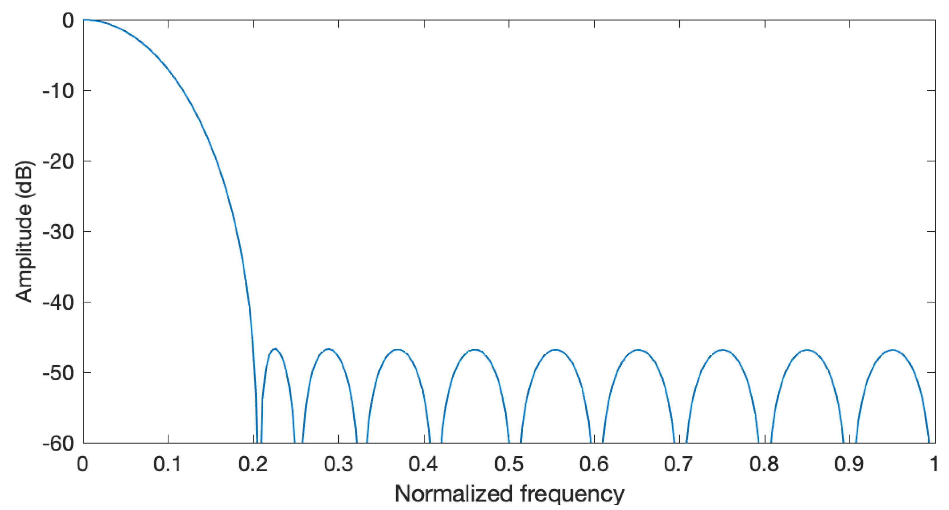
  • A simple yet effective interference detection technique using a low-pass filter is presented, and the presence of interference is further determined from the statistics of the output envelope of this filter. In this way, the results of interference detection can indicate the presence or absence of interference. We propose an interference mitigation algorithm that cannot be started in the absence of interference, which significantly increases real-time processing performance.
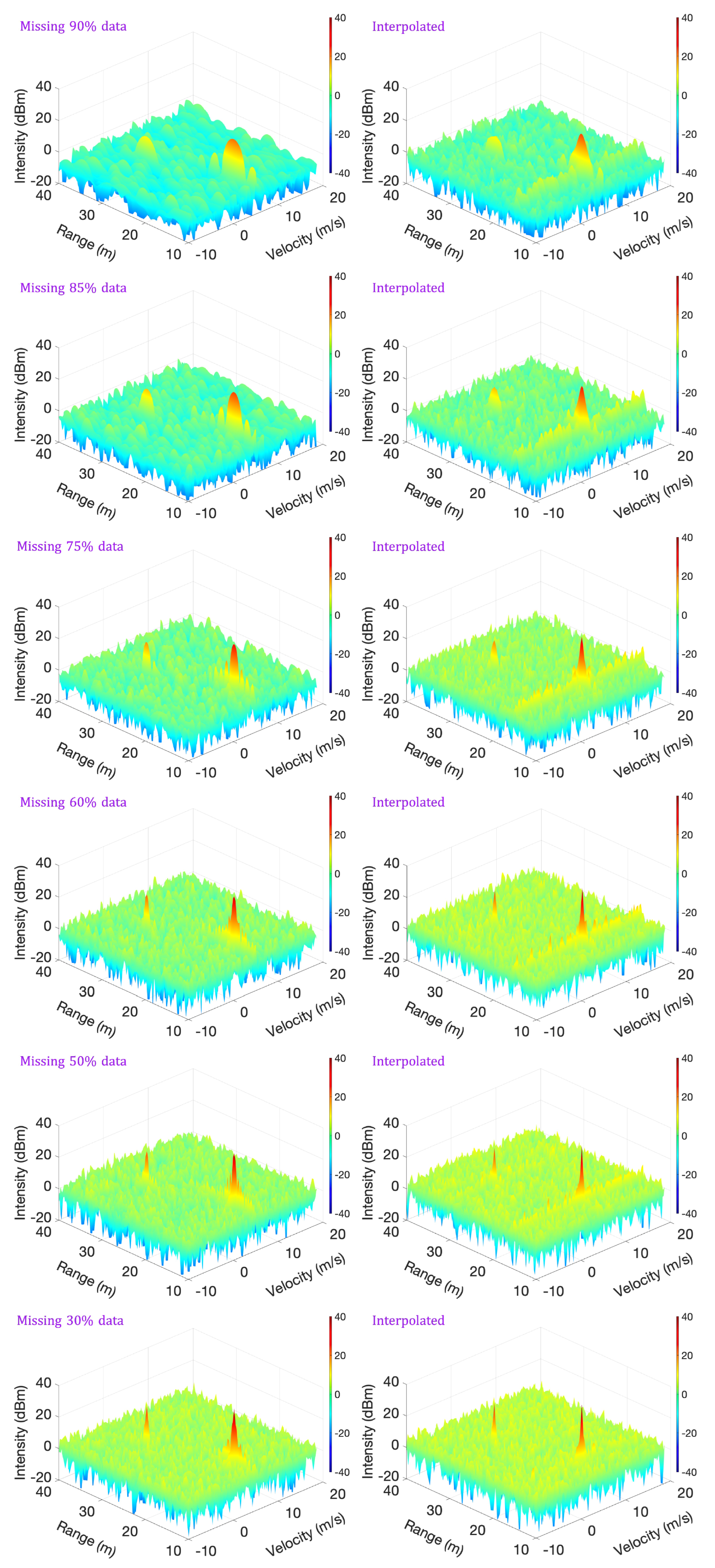
  • A sparsity model is presented to reduce the incoherent interference by considering the interference regions as missing data. Using L1 norm-regularized least squares, an alternating direction method of multipliers (ADMM)-based technique is been derived to restore the radar echoes.
  • In several comparison experiments, dynamic incoherent interference is generated; the case of dynamic interference is much closer to the real-world self-driving situation. In experiments with dynamic interference signals, the comparative performance of different algorithms is comprehensively evaluated and the potential use of the algorithms in real roads is further analyzed.
  • In addition, both the wavelet-based [19] and the MCA-based [23] methods are improved when using our proposed interference envelop detection approach.
  • Our extensive experiments demonstrate that the proposed method significantly outperforms the state-of-the-art methods on both simulated and real radar interference mitigation tasks.
The rest of this paper is outlined as follows. Section 2 introduces the formulations related to the incoherent interference between FMCW radars. Section 3 proposes detection and mitigation of incoherent interference. Section 4 demonstrates the extensive measurements used to compare the proposed techniques with state-of-the-art methods. Section 5 discusses sparsity-based methods, algorithm complexity, and the impact on performance of interference regions that lead to missing data components. Finally, we present our conclusions in Section 6.

2. Incoherent Interference

According to recommendations by the International Telecommunication Union (ITU), most automotive radars currently operate within the 76–81 GHz bandwidth with FMCW signals [26]. The transmitted radar signal s tx ( t ) can be written as follows:
s tx ( t ) = A tx cos ( 2 π f c t + π k r t 2 ) ,
where t is time, A tx is the amplitude of the transmitted signal, f c is the center frequency of the radar, and k r is the chirp rate. Suppose a vehicle at a distance R meters from the radar is driving at a speed v m/s; then, the corresponding radar echo is described as
s rx ( t ) = A rx cos [ 2 π f c ( t Δ t ) + π k r ( t Δ t ) 2 ] ,
where A rx is the amplitude of the echo, the delay time Δ t = 2 ( R + v t ) / c , and c is the velocity of light.
After the dechirp operation, the received signal is expressed as
r t ( t ) = A t cos ( 2 π Δ t k r t + ϕ r ) ,
where A t is the amplitude of the received signal and ϕ r is the phase that includes the target Doppler information. The frequency of the target signal with respect to time t is further derived as
f t ( t ) = Δ t k r .
If the neighboring radars and the radar under test have the same transmit waveform, then coherent interference may appear; false targets are generated when this type of interference signal enters the radar receiver baseband. Fortunately, this kind of interference is very unlikely to happen because the phase noise between the radar under test and interfering radars is not correlated. The transmitted signal of a neighboring radar is formulated as
s txi ( t ) = A txi cos [ 2 π f i ( t + t 0 ) + π k i ( t + t 0 ) 2 ] ,
where t 0 is the time offset with the radar under test as the reference, A txi is the amplitude, f i is the center frequency, and k i is the chirp rate for the neighboring radar.
When the transmitted signal of the neighboring radar passes through the receiver of the radar under test, the interfering signal after dechirping is
r i ( t ) = A i cos [ 2 π ( f c f i ) t + π ( k r k i ) t 2 2 π k i t 0 t + ϕ i ] ,
where A i and ϕ i are the amplitude and residual phase of the interfering signal, respectively. According to the above equation, the frequency of the interfering signal with respect to time t is
f i ( t ) = f c f i k i t 0 + ( k r k i ) t .
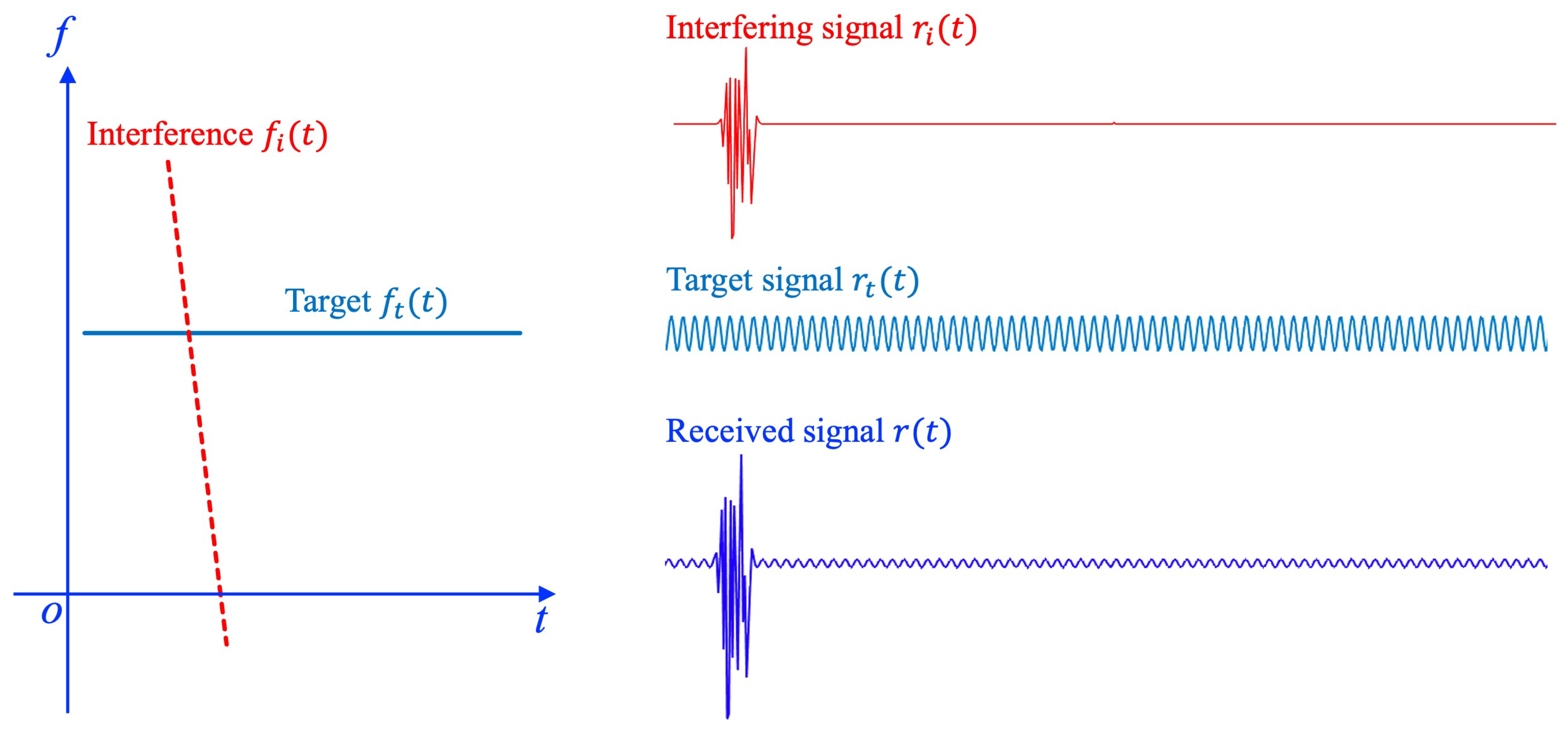
It can be seen that the above interfering signal is a linear FM signal, which is called incoherent interference. The part of the interfering signal with a frequency below half of the radar receiver sampling frequency is fully sampled, and the rest above it is undersampled.
The total received signal can be considered as the sum of the target signal and the interfering signal, that is, r ( t ) = r t ( t ) + r i ( t ) , as shown in Figure 1. It is worth mentioning that the power of the target signal is proportional to R 4 while the amplitude of the interference is proportional to R i a , where a is a factor that describes the multi-path transmission of the interfering signal and R i is the distance between the interfering radar and the radar under test. Low-intensity incoherent interference signals have little effect on radar performance, and only raise the noise floor. In this work, the intensity of the interfering signal is considered to be stronger than that of the target signal, which makes it difficult to suppress the interference. Therefore, 2 a < 4 .

3. Proposed Approaches

3.1. Interference Envelope Detection

Interference envelope detection is the first priority in interference mitigation. The precise location of the interference facilitates the reduction of interference with minimal computational complexity. After discrete-time quantization sampling, the received signal can be described as r ( n ) , where n denotes the nth sample. First, the amplitude information is obtained by taking the modulus of the radar received signal as
A r ( n ) = | r ( n ) | .
Next, one low-pass finite impulse response filter (LP-FIR) is designed to detect the envelop. The frequency response of the filter is
H ( ω ) = n = 0 K h n e j n ω ,
where K is the order of the filter and h n is a coefficient of the filter. Thus, the impulse response of the filter can be written as
h ( n ) = i = 0 K h i δ [ n i ] = h n , 0 n K .
There are many methods that can be used to solve the filter coefficients, such as the window function method and the frequency sampling method [27]. Here, a minimum mean square error (MMSE)-based method is applied to design the filter.
To simplify the design, h ( n ) is expected to be even symmetric and the order K is set as an odd number. Hence, the discrete-time Fourier transform (DTFT) of h ( n ) can be rewritten as
H ( ω ) = e j ω ( N + 1 ) / 2 n = 0 ( K + 1 ) / 2 h n cos ω K + 1 2 n ,
According to the above equation, the phase response of the filter is ϕ ( ω ) = e j ω ( K + 1 ) / 2 . Thus, a desired filter H d ( ω ) can be predefined by combining the phase response ϕ ( ω ) with a desired amplitude response. The design of the filter can then be further expressed as an MMSE problem:
min h ( n ) E ( ω ) = π / 2 π / 2 H ( ω ) H d ( ω ) 2 d ω .
The above problem is minimized by applying the partial derivative of E ( ω ) with respect to h ( n ) to obtain the solution,
h ( n ) = π / 2 π / 2 cos ( n ω ) H d ( ω ) d ω .
Because the frequency of the interference envelope is low, the normalized cutoff frequency of the filter is set to 0.2, the passband normalized frequency is 0.005, the order of the filter is set to 19, and a filter coefficient vector is designed: h ( n ) = 0.01 * [ 0.59 , 1.08 , 1.91 , 2.99 , 4.25 , 5.61 , 6.94 , 8.10 , 8.97 , 9.43 , 9.43 , 8.97 , 8.10 , 6.94 , 5.61 , 4.25 , 2.98 , 1.91 , 1.08 , 0.59 ] . The amplitude response of the filter is shown in Figure 2.
Applying the designed filter to the amplitude sequence, the envelope A ( n ) can be obtained:
A ( n ) = k = 0 N 1 h ( k ) A r ( n k ) ,
where N is the length of the received signal.

3.2. Generating Missing Data for Interference Regions

The method for detecting of the interference envelope described above applies to all the received signals. Next, it is necessary to determine whether there is interference in the received signal. Because the target echo signals are superimposed as complex sine waves, the mean and maximum values of the echo amplitude do not differ very much. However, according to a large number of experiments, the maximum value of the interfering signal amplitude is at least three times larger than the mean value of the echo amplitude; thus, the presence of interference is determined by
label inter = 1 max ( | A ( n ) | ) > 3 * mean ( | A ( n ) | ) , 0 otherwise .
In addition, the label inter label indicates whether the proposed data interpolation algorithm is stopped or started, reducing the processing complexity. Then, the nth received signal sample is further determined as either an affected or unaffected sample according to the following equation:
z ( n ) = 1 label inter & | A ( n ) | > β * mean ( | A ( n ) | ) , 0 otherwise .
where β is a parameter that depends on the power of the interference.
The interfering areas are then set to be missing data:
y * ( n ) = 0 z ( n ) = 1 , r ( n ) z ( n ) = 0 .
In keeping with the above equations, Figure 3 presents the detected interference envelope and the received signal with missing data. As can be seen from the plots, the proposed method is able to effectively detect four interference regions and accurately identify the affected samples. As plotted in Figure 4, in the absence of interference the proposed approach accurately sets label inter as 0, the received signal is identified as the target signal, and no further interference detection or mitigation is required.

3.3. Data Interpolation Using L1 Norm Least Squares Method

Suppose the length of a signal y ( n ) is N; then, the M-point ( M N ) inverse DFT of the signal y ( n ) is defined as follows:
y = Wx ,
where
W = 1 M 1 1 1 1 e j 2 π M e j ( M 1 ) 2 π M 1 e j ( N 1 ) 2 π M e j ( N 1 ) ( M 1 ) 2 π M ,
y = [ y ( 0 ) , y ( 1 ) , , y ( N 1 ) ] T , and the DFT coefficients x = [ x ( 0 ) , x ( 1 ) , , x ( M 1 ) ] T .
Therefore, the DFT coefficient is expressed as
x = W H y ,
with
W H = 1 1 1 1 e j 2 π M e j ( N 1 ) 2 π M 1 e j ( M 1 ) 2 π M e j ( M 1 ) ( N 1 ) 2 π M ,
and W W H = I .
In the above discussion the target signal is in the form of a complex sine wave, and is therefore sparse in the DFT domain. Thus, the problem of missing data imputation can be formulated with the L1 norm as
arg min x x 1 , s . t . y * = z ( Wx ) ,
where y * = [ y * ( 0 ) , y * ( 1 ) , , y * ( N 1 ) ] T , and z = [ z ( 0 ) , z ( 1 ) , , z ( N 1 ) ] T .
The target signal with missing data can be reconstructed by minimizing the objective function:
J ( x ) = 1 2 y * z ( Wx ) 2 2 + λ x 1 ,
where λ is the parameter for the L1 norm term.
The above object function can be further rewritten as
arg min x J ( x ) , s . t . x v = 0 ,
where v is a new variable vector.
Using the augmented Lagrangian method, the above problem is formulated as
L A ( x , λ , μ ) = J ( x ) + λ ( x v ) + μ 2 x v 2 2 ,
where μ 0 is a penalty parameter. ADMM is applied to perform minimization with respect to each of x and v to obtain the following iterations:
x k = arg min x λ x 1 + μ 2 x v k d k 2 2 , v k = arg min v 1 2 y * z ( Wx k ) 2 2 + μ 2 x k v d k 2 2 , d k + 1 = d k ( x k v k ) ,
where k is the iteration number and d k is an intermediate variable vector.
First, minimization with respect to x is implemented using a soft thresholding:
x k = soft v k + d k , λ 2 μ ,
where the soft thresholding operation is defined as
soft ( x , Ø ) = x · max 1 Ø / | x | , 0 .
Next, minimization with respect to v is a constrained least squares regularization. Because W W H = I , the solution can be simplified as
v k = W H y * z ( Wx k ) .
Finally, after convergence of the solution, the estimated received signal is obtained by
y ^ = Wx k .

3.4. Implementation Details

Figure 5 summarizes the procedures of the proposed techniques. Each echo is processed one by one, then the DFT-based image focusing algorithm is used to focus the radar target, and finally a radar image without interference contamination is obtained. In the radar image focusing algorithm, the data focus is directed to the the ranging and Doppler domains by applying the Fast Fourier Transform (FFT) method. The vectors v k and d k are set as zero for the first iteration. Because the intensity of radar echoes is small, the parameters in Equation (24) can be set according to the mean value of the radar echoes; specifically, λ can be set to 1 and μ can be set to be proportional to the inverse of the mean intensity of the received signal. Additionally, the iteration number for missing data imputation can be set as 20, which produces satisfactory performance.

4. Validation Experiments

In the following experiments, the proposed technique is compared with three state-of-the-art methods. The first approach is one of the simplest ubiquitous signal processing methods, substituting zeros for the interference regions [15]. The second one represents a more advanced signal processing method using a three-level Haar wavelet with the hard thresholding approach [19]. The final comparison is a sparsity-based MCA method that uses DFT and STFT bases to separate the interfering and target signals, respectively [23]. In the following comparison experiments, the parameters of the wavelet-based and MCA-based methods are set according to references [19] and [23], respectively.
Furthermore, both the wavelet-based [19] and MCA-based [23] methods are improved using the proposed interference envelop detection. Specifically, based on the results of our proposed interference envelope detection method, only the signals in the interference regions are replaced by the outputs of the wavelet and MCA methods.
The comparisons are divided into three groups: stationary interference experiments, dynamic interference experiments, and real radar interference experiments. The first two types of experiments are implemented by simulations. In the following experiments, both the radar under test and the interfering radar are static and the targets are moving. For the stationary interference experiments, the timing between the victim and interfering radars is synchronized, and the jamming appears in the same area of the received signal. In practice, timing synchronization between radars rarely occurs due to relative motion between the radar under test and the interfering radar, making dynamic interference common. As a result, interference appears in different regions in the received signal of the radar under test. Due to the constraints of the experimental conditions, the radar senors in the described experiments are static; however, the timing between the victim and interfering radars is set asynchronously in order to simulate dynamic interference.
Additionally, thermal noise is added to the simulated signals. The power of the noise was calculated as P nosie = κ T e B , where κ is Boltzman’s constant, T e is the noise temperature, and B is the bandwidth of the radar receiver.
In the case of one-dimensional signals, the signal to interference plus noise ratio (SINR) is used to objectively evaluate the performance of interference suppression. However, for two-dimensional radar images, the radar target is focused through two dimensional range and Doppler domains. Therefore, the peak intensity of the target to interference plus noise ratio (PTINR) is defined here as an objective evaluation index for interference mitigation. Using the peak intensity of the focused target, the PTINR is defined as
PTINR = P target P interference + P noise ,
where P target is the peak intensity (power) of the focused target and P interference is the power of the interference.
In addition, the subjective evaluation of radar images is mainly based on the quality of the focused target, sidelobes of the focused target, noise floor level, and residual interference distribution as comparative details.

4.1. Simulations

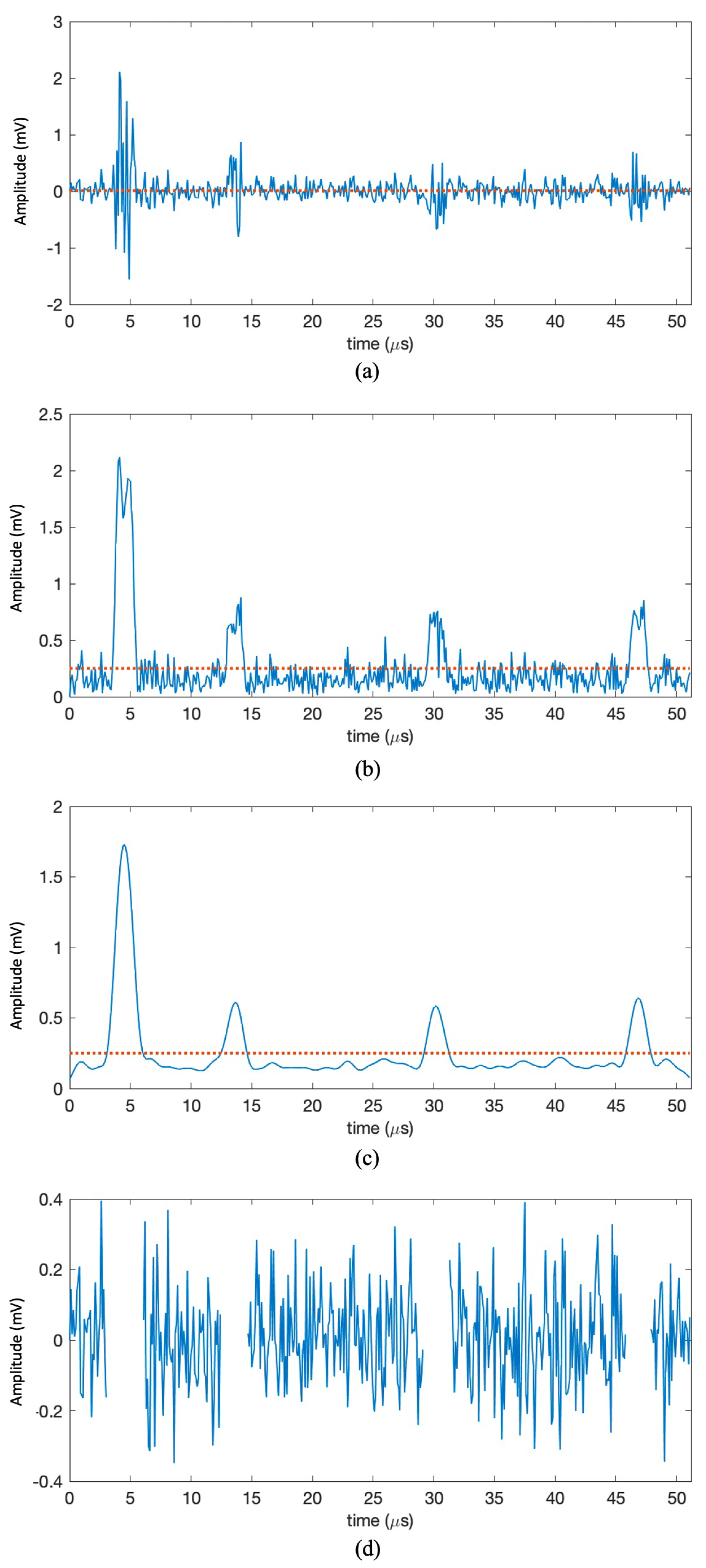
Table 1 provides the simulation parameters for the incoherent interference experiments. Two interfering sources are developed with different start frequencies and chirp rates. The distances of the two interfering sources are 30 m and 50 m from the radar under test, respectively. All the radar sensors are active at the same time. The RCS is 1 m 2 and 3 m 2 for two radar targets at 15 m and 30 m, respectively. The target located at 15 m is moving at 5 m/s, while the other target is static. As shown in 
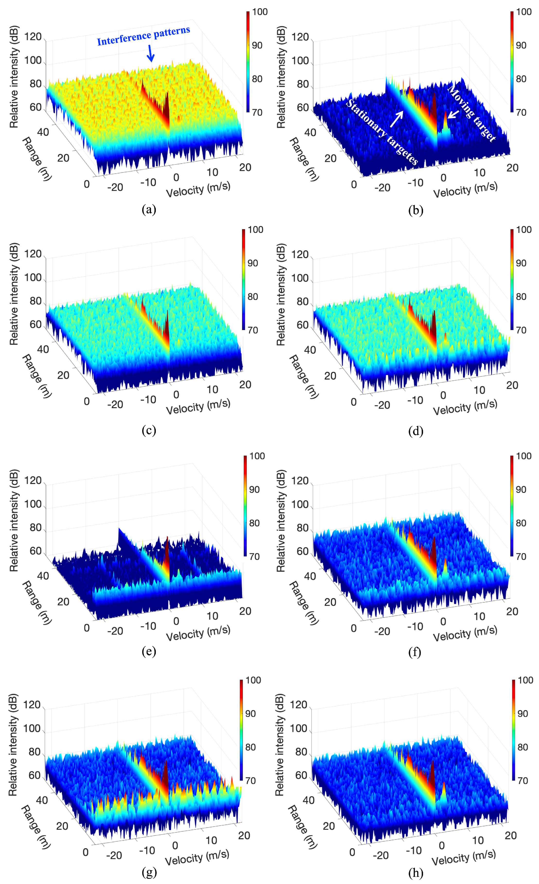
Figure 6, there are four interference regions present in the received signal.
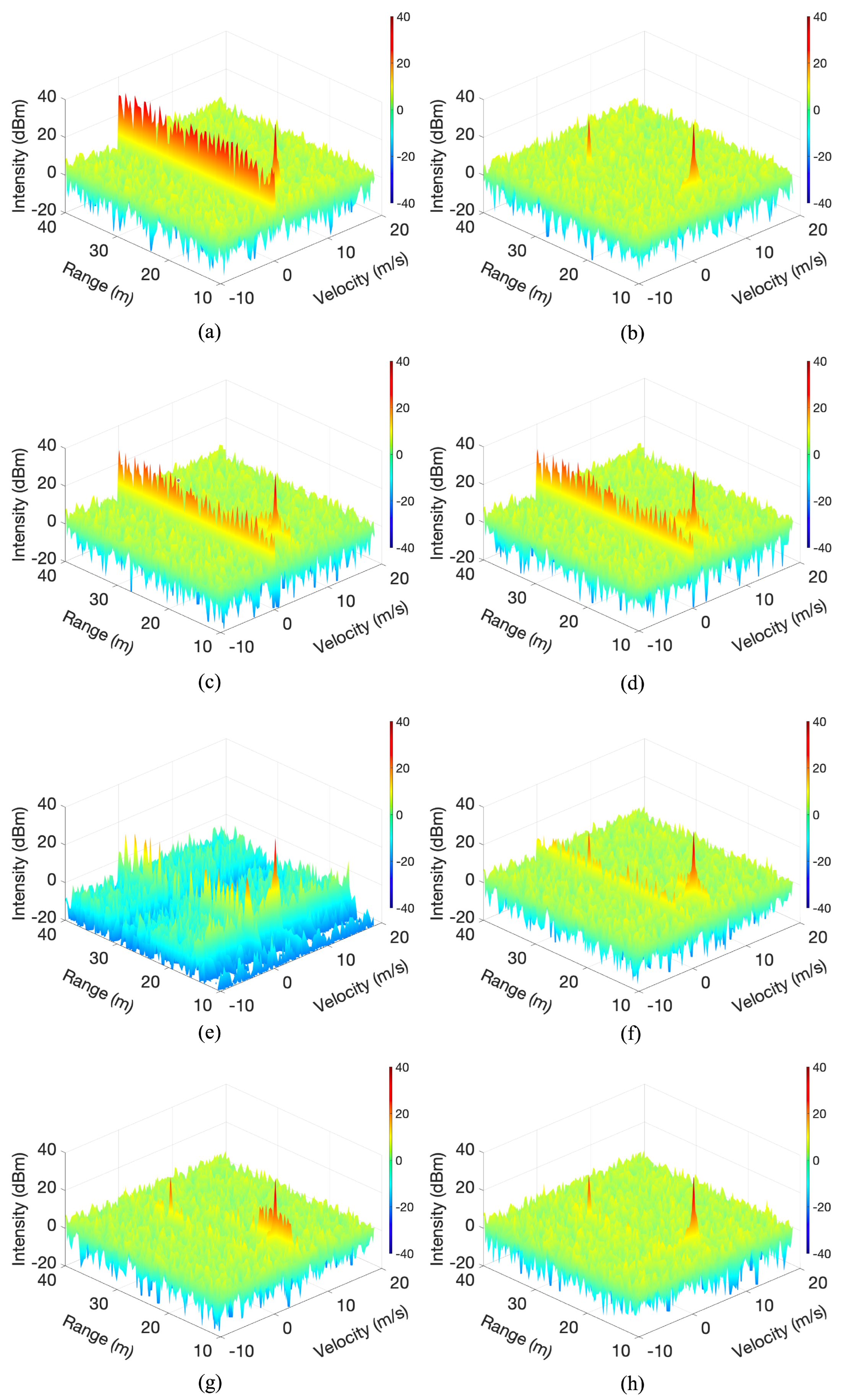
Figure 7 illustrates the comparative stationary interference experiments. According to Figure 7a, the stationary interference is distributed on the axis of zero velocity of the focused image, causing the second target to be completely swamped by the large amount of strong noise generated on this axis. Traditional signal processing-based methods such as the ANC and wavelet-based methods are able to suppress the interfering signal to a certain extent. However, the interfering signal is much stronger than the target signal, making it difficult to suppress the interference by traditional signal processing methods, as shown in the plots. Figure 7c illustrates that the wavelet-based approach has difficulty suppressing this strong interference. Using the proposed interference envelope method, the improved wavelet-based method does not perform better; see Figure 7d. This means that the reference regions have not been successfully recovered. Although the MCA method provides slightly better results (Figure 7e), there is a considerable amount of interference energy left in the zero velocity axis, resulting in failure to detect the second radar target. After introducing the proposed interference envelope detection method to improve the MCA method, both targets are successfully recovered and the interference signal energy is more effectively eliminated, as shown in Figure 7f. Figure 7g shows that the simple zero-setting method avoids the interfering signal. However, due to the loss of the target signal in the interfering regions, it leads to strong sidelobes in the focused image. According to 
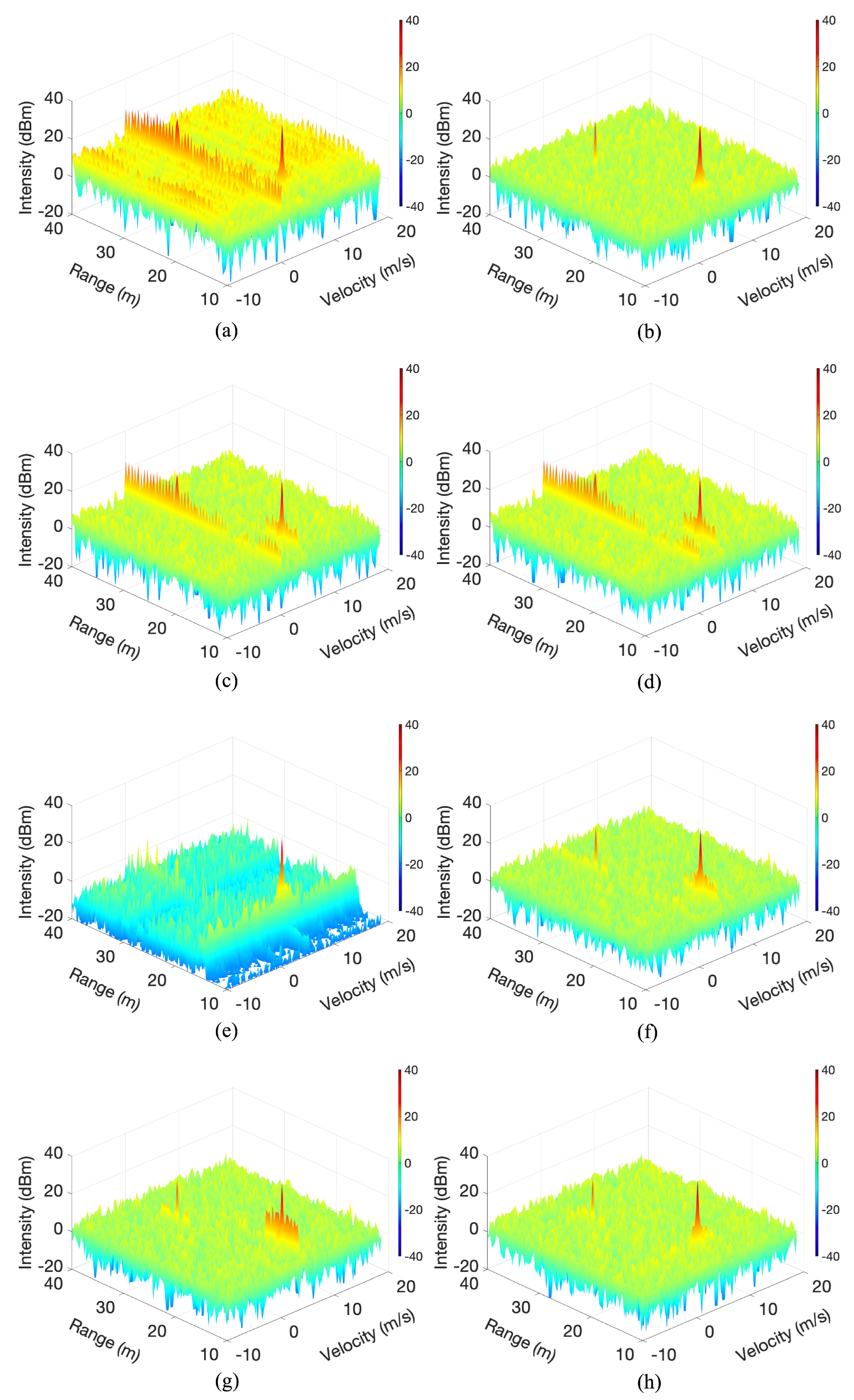
Figure 7h, the proposed method produces a promising focused image that is very close to the ground truth. In many real-world vehicle scenarios, the primary and interfering radars have relative motion, producing dynamic interference. Compared with stationary interference, the interference energy from dynamic interference is distributed in different areas on the focused image; see Figure 8a. As the interference energy is distributed in different regions of the image, the interference intensity is relatively lower, and the different interference suppression algorithms consequently have better performance for dynamic interference suppression, as shown in Figure 8. Similarly, the proposed interference envelope detection approach greatly improves the performance of the MCA method; see Figure 8f. Again, as illustrated in Figure 8h, the proposed approach produces the most focused radar image.
Comparisons of object evaluation were conducted as well. The results are reported in Table 2. The larger PTINRs along with the absence of ghost targets indicate the better suppression performance of the associated method. The proposed method has the best performance index in the simulated experiments. Because the static target appears on the zero velocity line axis of the focused image, and is therefore covered by strong interference energy, its PTINR value is −6.1 dB. The wavelet-based method and MCA-based method have limited improvement on this index, while the proposed method can realize an improvement of up to 19.1 dB, a total improvement of 25.2 dB, which is beneficial for subsequent target detection and tracking.

4.2. Real Radar Field Experiments
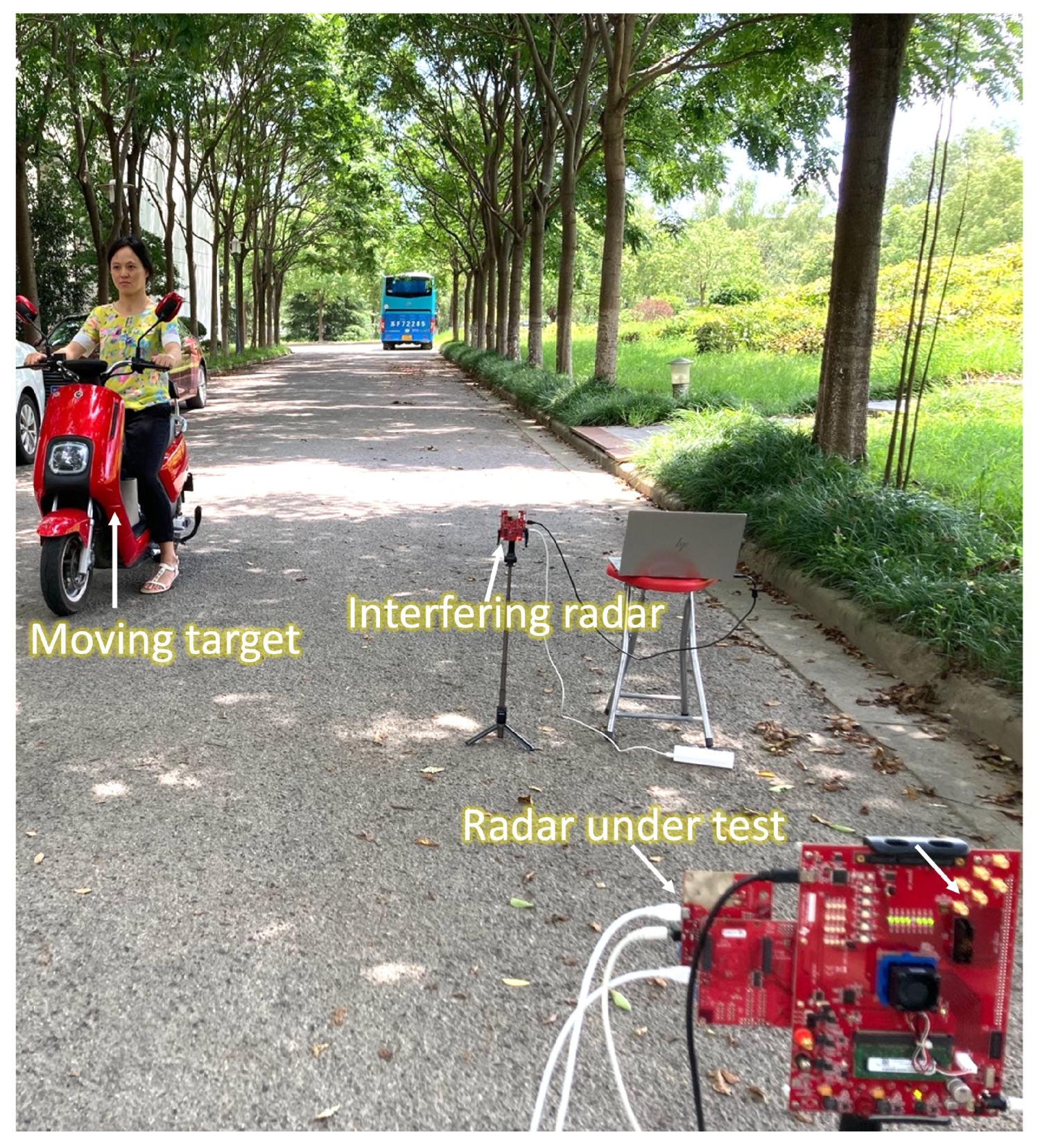
As shown in Figure 9, real radar interference experiments were conducted using two Texas Instruments AWR1642 mm wave radars and an electric bicycle traveling at approximately 5 m/s forward or backward relative to the radar under test. The distance of the interfering radar was 4 m. The experiment parameters are presented in Table 3.
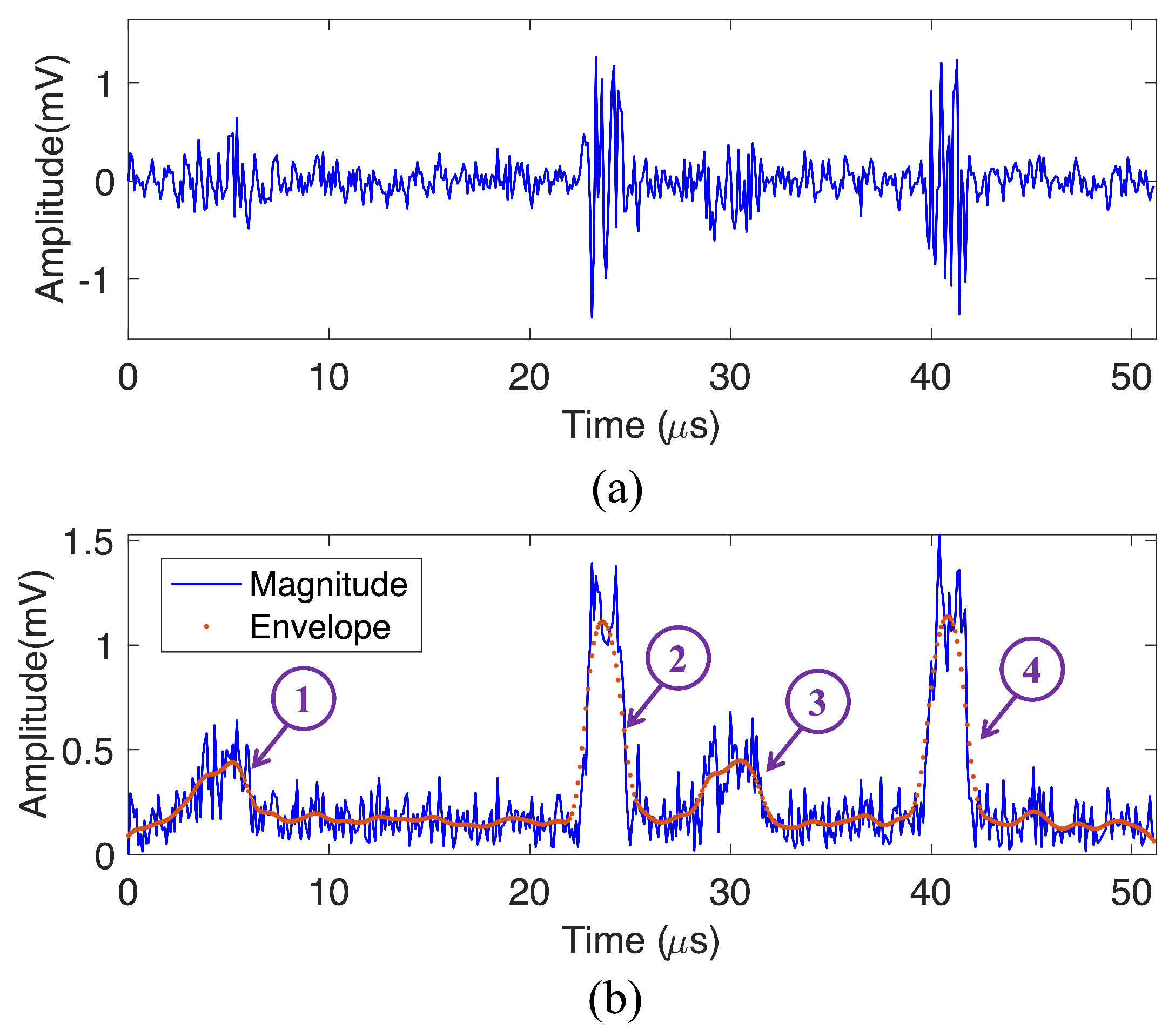
Figure 10 demonstrates the collected radar data with strong interference. The signal of the sine wave in the plot is the radar target signal, and the signal that changes suddenly and quickly with high intensity is the interfering signal. This coincides with the theoretical derivation in Section 2.
Figure 11 presents the comparison results of the real radar interference experiments. The stationary targets are distributed on the axis of zero velocity of the focused image, however the moving target is not visible due to strong interference. Compared to the other approaches, the proposed method has the best performance. As shown in Figure 11a, the strong interference energy is distributed over the focused radar image. The main reason for this is that the interfering signal does not repeat at the same location in each received signal with dynamic interference. Compared to the simulated results, the zeroing method produces stronger sidelobes on the focused image, which leads to difficulty in distinguishing between real moving targets; see Figure 11g. The evaluation results reported in Table 4 indicate that the proposed method has the best performance index in the real radar experiments.

5. Discussion

5.1. Beyond Sparsity-Based Methods

Certain radar targets have a large radar cross-section (RCS), such as metal buildings on the side of a road, while others have a small RCS, such as pedestrians. All in all, the dynamic range of the received signal is large. Therefore, it is difficult to extract weak targets in an interference environment. Unfortunately, sparsity-based methods have a general drawback in that they tend to remove weak signals as noise. As shown in Figure 7, Figure 8, and Figure 10, the traditional sparsity-based method [23] can only recover strong targets, and loses weak targets. The proposed method, although retaining a sparse framework, proposes an interference detection method that enables signal recovery only for the region where the interference occurs, thus effectively maintaining the signal energy and suppressing the interference signal at the same time.

5.2. Computational Complexity

The complexity of the interference suppression algorithm needs to be as small as possible in order to be suitable for the signal processor of existing automotive millimeter wave radar chips. Therefore, interference-contaminated region detection-based methods have advantages in terms of computing complexity. Zero-based detection methods simply set the interference-contaminated regions to zero, and thus have the least complexity. However, the focused target obtained with such methods loses information and has many sidelobes.
Except for the zeroing method, the wavelet-based method [19], the MCA-based method [23], and the proposed technique are all transform-based approaches, meaning that the computational complexity depends mainly on forward and inverse transformation. In general, the wavelet-based method has the lowest complexity, followed by the proposed method. The MCA method has the highest computational complexity due to the use of both STFT and DFT [23].

5.3. What Is the Percentage of Samples Affected by Interference for Which the Proposed Technique Remains Valid?

In the proposed technique, a greater proportion of interfering samples produce fewer effective received samples, thereby reducing range resolution and signal-to-noise ratio. Therefore, we conducted experiments to investigate the performance of the proposed technique with respect to the differing percentage of interfering samples. According to Figure 12 and Figure 13, when the percentage of interfering samples is below 50%, the performance of the proposed method is satisfactory. The interference signal is generally in the shape of a burst in the time domain, and rarely occupies most of the received signal, allowing the proposed method to cope with the interference in most cases.

6. Conclusions

In this paper, an effective and feasible interference suppression technique is proposed for the currently important and challenging issue of incoherent interference between automotive FMCW radars. A detailed derivation of the processing of incoherent interference signals is presented. A precise interference envelope detection method is proposed based on a well-designed low-pass filter. This method can avoid interference suppression in cases where the signal is received without interference, thereby reducing the required amount of computation. This work considered the interference problem as a missing radar data problem; the radar target signal is superimposed in complex sinusoidal waves with good sparse characteristics in the DFT domain. Thus, the radar target signal polluted by the incoherent interference can be successfully recovered based on the L1 norm least squares method. Using the proposed method, the radar target can be perfectly focused even in cases of strong interference. Moreover, two current state-of-the-art methods, namely, the wavelet-based and MCA-based methods, are improved when using the proposed interference envelope detection method. Extensive experiments demonstrate the promising performance of the proposed techniques.
This work shows the effectiveness of suppressing interference in the range and Doppler domains. However, this work does have limitations; in particular, it does not investigate interference in spatial multi-channel data. Our future work will focus on interference reduction for spatial multi-channel radar data.

Author Contributions

Conceptualization, Z.X.; methodology, Z.X. and Y.W.; software, Y.W.; validation, S.X. and Y.W.; experimental analysis, S.X.; data collection, Z.X., S.X. and Y.W.; writing—original draft preparation, Y.W.; writing—review and editing, Z.X.; supervision, Z.X. All authors have read and agreed to the published version of the manuscript.

Funding

This work was supported by the National Natural Science Foundation of China (Grant number 42005100) and by the Nantong Science and Technology for Social and Livelihood Key Project (Grant number MS22022016).

Data Availability Statement

Not applicable.

Acknowledgments

Although this work was supported by two projects, the remaining costs of the project did not cover article processing charges for the paper. The editorial team of Remote Sensing has been very supportive and helpful. Your journal’s timely help made us feel sunshine and warmth in the midst of much-needed help, and and we will continue to do meaningful and interesting works and apply for relevant grants in return for our scientific journal and the kind people and well-wishers around the world. In addition, the authors would like to express their sincere gratitude to the editors and reviewers whose insightful comments have further enhanced the quality of the paper.

Conflicts of Interest

The authors declare no conflict of interest.

References

  1. Gardill, M.; Schwendner, J.; Fuchs, J. An Approach to Over-the-air Synchronization of Commercial Chirp-Sequence Automotive Radar Sensors. In Proceedings of the 2020 IEEE Topical Conference on Wireless Sensors and Sensor Networks (WiSNeT), San Antonio, TX, USA, 26–29 January 2020; pp. 46–49. [Google Scholar] [CrossRef]
  2. Jasteh, D.; Hoare, E.G.; Cherniakov, M.; Gashinova, M. Experimental Low-Terahertz Radar Image Analysis for Automotive Terrain Sensing. IEEE Geosci. Remote. Sens. Lett. 2016, 13, 490–494. [Google Scholar] [CrossRef]
  3. Xu, Z.; Baker, C.J.; Pooni, S. Range and Doppler Cell Migration in Wideband Automotive Radar. IEEE Trans. Veh. Technol. 2019, 68, 5527–5536. [Google Scholar] [CrossRef]
  4. Patole, S.M.; Torlak, M.; Wang, D.; Ali, M. Automotive radars: A review of signal processing techniques. IEEE Signal Process. Mag. 2017, 34, 22–35. [Google Scholar] [CrossRef]
  5. Alland, S.; Stark, W.; Ali, M.; Hegde, M. Interference in automotive radar systems: Characteristics, mitigation techniques, and current and future research. IEEE Signal Process. Mag. 2019, 36, 45–59. [Google Scholar] [CrossRef]
  6. Tovar Torres, L.L.; Steiner, M.; Waldschmidt, C. Channel Influence for the Analysis of Interferences Between Automotive Radars. In Proceedings of the 2020 17th European Radar Conference (EuRAD), San Antonio, TX, USA, 26–29 January 2020; pp. 266–269. [Google Scholar] [CrossRef]
  7. Torres, L.L.T.; Roos, F.; Waldschmidt, C. Simulator Design for Interference Analysis in Complex Automotive Multi-User Traffic Scenarios. In Proceedings of the 2020 IEEE Radar Conference (RadarConf20), Florence, Italy, 21–25 September 2020; pp. 1–6. [Google Scholar] [CrossRef]
  8. Hua, X.; Ono, Y.; Peng, L.; Xu, Y. Unsupervised Learning Discriminative MIG Detectors in Nonhomogeneous Clutter. IEEE Trans. Commun. 2022, 70, 4107–4120. [Google Scholar] [CrossRef]
  9. Rosenberg, L.; Bocquet, S. Non-coherent Radar Detection Performance in Medium Grazing Angle X-Band Sea Clutter. IEEE Trans. Aerosp. Electron. Syst. 2017, 53, 669–682. [Google Scholar] [CrossRef]
  10. Xu, Z.; Shi, Q.; Shi, J.; Wang, H.; Wei, M.; Gao, R.; Shao, Y.; Tao, H. A novel method of mitigating the mutual interference between multiple LFMCW radars for automotive applications. In Proceedings of the IGARSS 2019–2019 IEEE International Geoscience and Remote Sensing Symposium, Yokohama, Japan, 28 July–2 August 2019; pp. 2178–2181. [Google Scholar]
  11. Xu, Z.; Shi, Q. Interference mitigation for automotive radar using orthogonal noise waveforms. IEEE Geosci. Remote Sens. Lett. 2018, 15, 137–141. [Google Scholar] [CrossRef]
  12. Xu, Z.; Shi, Q.; Sun, L. Novel Orthogonal Random Phase-Coded Pulsed Radar for Automotive Application. J. Radars 2018, 7, 364–375. [Google Scholar] [CrossRef]
  13. Uysal, F. Phase-coded FMCW Automotive Radar: System Design and Interference Mitigation. IEEE Trans. Veh. Technol. 2019, 69, 270–281. [Google Scholar] [CrossRef]
  14. Yuan, M.; Xu, Z.; Shi, Q. Wiener filter based automotive millimeter wave radar interference adaptive reduction. J. Electron. Meas. Instrum. 2021, 35, 194–201. [Google Scholar] [CrossRef]
  15. Brooker, G.M. Mutual Interference of Millimeter-Wave Radar Systems. IEEE Trans. Electromagn. Compat. 2007, 49, 170–181. [Google Scholar] [CrossRef]
  16. Neemat, S.; Krasnov, O.; Yarovoy, A. An interference mitigation technique for FMCW radar using beat-frequencies interpolation in the STFT domain. IEEE Trans. Microw. Theory Techn. 2019, 67, 1207–1220. [Google Scholar] [CrossRef]
  17. Jung, J.; Lim, S.; Kim, J.; Kim, S.C.; Lee, S. Interference Suppression and Signal Restoration Using Kalman Filter in Automotive Radar Systems. In Proceedings of the 2020 IEEE International Radar Conference (RADAR), Washington, DC, USA, 28–30 April 2020; pp. 726–731. [Google Scholar]
  18. Wang, J.; Ding, M.; Yarovoy, A. Matrix-Pencil Approach-Based Interference Mitigation for FMCW Radar Systems. IEEE Trans. Microw. Theory Techn. 2021, 69, 5099–5115. [Google Scholar] [CrossRef]
  19. Lee, S.; Lee, J.Y.; Kim, S.C. Mutual Interference Suppression Using Wavelet Denoising in Automotive FMCW Radar Systems. IEEE Trans. Intell. Transp. Syst. 2021, 22, 887–897. [Google Scholar] [CrossRef]
  20. Jin, F.; Cao, S. Automotive Radar Interference Mitigation using Adaptive Noise Canceller. IEEE Trans. Veh. Technol. 2019, 68, 3747–3754. [Google Scholar] [CrossRef]
  21. Wu, J.; Yang, S.; Lu, W.; Liu, Z. Iterative modified threshold method based on EMD for interference suppression in FMCW radars. IET Radar Sonar Navig. 2020, 14, 1219–1228. [Google Scholar] [CrossRef]
  22. Xu, Z.; Yuan, M. An Interference Mitigation Technique for Automotive Millimeter Wave Radars in the Tunable Q-Factor Wavelet Transform Domain. IEEE Trans. Microw. Theory Techn. 2021, 69, 5270–5283. [Google Scholar] [CrossRef]
  23. Uysal, F. Synchronous and asynchronous radar interference mitigation. IEEE Access 2018, 7, 5846–5852. [Google Scholar] [CrossRef]
  24. Afonso, M.V.; Bioucas-Dias, J.M.; Figueiredo, M.A. Fast image recovery using variable splitting and constrained optimization. IEEE Trans. Image Process. 2010, 19, 2345–2356. [Google Scholar] [CrossRef]
  25. Rock, J.; Roth, W.; Toth, M.; Meissner, P.; Pernkopf, F. Resource-Efficient Deep Neural Networks for Automotive Radar Interference Mitigation. IEEE J. Sel. Top. Signal Process. 2021, 15, 927–940. [Google Scholar] [CrossRef]
  26. International Telecommunication Union. Systems Characteristics of Automotive Radars Operating in the Frequency Band 76–81 GHz for Intelligent Transport Systems Applications; Mobile, Radiodetermination, Amateur and Related Satellite Service; International Telecommunication Union: Geneva, Switzerland, 2018. [Google Scholar]
  27. Kidambi, S. Design of Noise Transfer Functions for Delta–Sigma Modulators Using the Least-pth Norm. IEEE Trans. Circuits Syst. II Express Briefs 2019, 66, 707–711. [Google Scholar] [CrossRef]
Figure 1. Demonstration of incoherent interference.
Remotesensing 14 04817 g001
Figure 2. The amplitude response of the designed filter.
Remotesensing 14 04817 g002
Figure 3. In the presence of interference ( label inter = 1 ) : (a) the real part of the received signal; (b) the amplitude of the received signal; (c) the interference envelope detected by LPF; and (d) the received signal containing the affected samples. The dashed line in the subplots indicates the mean value of the corresponding signal.
Remotesensing 14 04817 g003
Figure 4. In the absence of interference ( label inter = 0 ) : (a) the real part of th received signal; (b) the amplitude of the received signal; (c) the echo envelope detected by LPF; and (d) the received signal that does not contain affected samples. The dashed line in the sub-figures indicates the mean value of the corresponding signal.
Remotesensing 14 04817 g004
Figure 5. The procedures of the proposed techniques.
Remotesensing 14 04817 g005
Figure 6. The received signal with interference: (a) the real part of the received signal and (b) the magnitude of the received signal. The regions marked by circles in (b) are the envelopes in which interference appears.
Remotesensing 14 04817 g006
Figure 7. Comparisons on stationary interference simulations. (a) Original image; (b) Interference-free image; (c) Lee et al. [19]; (d) Lee et al. [19] + Proposed interference detection; (e) Uysal [23]; (f) Uysal [23] + Proposed interference detection; (g) Brooker [15]; and (h) The proposed method.
Remotesensing 14 04817 g007
Figure 8. Comparisons on dynamic interference simulations. (a) Original image; (b) Interference-free image; (c) Lee et al. [19]; (d) Lee et al. [19] + Proposed interference detection; (e) Uysal [23]; (f) Uysal [23] + Proposed interference detection; (g) Brooker [15]; and (h) The proposed method.
Remotesensing 14 04817 g008
Figure 9. Real radar field experiments.
Remotesensing 14 04817 g009
Figure 10. The received signal during the measurement experiments: the plots on the top row is the real part of the signal, and the plots on the bottom row is the magnitude of the received signal.
Remotesensing 14 04817 g010
Figure 11. Comparisons using real radar data. (a) Original image; (b) Interference-free image; (c) Lee et al. [19]; (d) Lee et al. [19] + Proposed interference detection; (e) Uysal [23]; (f) Uysal [23] + Proposed interference detection; (g) Brooker [15]; and (h) The proposed method.
Remotesensing 14 04817 g011
Figure 12. The performance of the proposed technique with respect to different percentages of interfering samples.
Remotesensing 14 04817 g012
Figure 13. Comparison of range and Doppler profiles in terms of different percentages of interfering samples.
Remotesensing 14 04817 g013
Table 1. Simulation parameters for interference experiments.
RadarsParametersValues
Common parametersBandwidth500 MHz
Sampling rate10 Msps
Chirp number128
Radar under testStart frequency77 GHz
Chirp duration51.2 µs
Chirp rate9.76  × 10 12 Hz/s
Interferer 1Start frequency77.7 GHz
Chirp duration25.6 µs
Chirp rate−1.95  × 10 13 Hz/s
Distance30 m
Interferer 2Start frequency76.9 GHz
Chirp duration17.07 µs
Chirp rate2.93  × 10 13 Hz/s
Distance50 m
Table 2. Comparisons of PTINRs via simulations. The first number in each term is the result of stationary interference and the second number is the result of dynamic interference.
MethodsTarget 1Target 2
(dB)(dB)
Original image25.6, 29.8−6.1, 6.2
Ground truth without interference36.825.5
Lee et al. [19]24.9, 30.2−3.3, 14.9
Lee et al. [19] + the proposed interference detection26.5, 30.8−2.7, 20.3
Uysal [23]26.4, 28.93.1, 12.5
Uysal [23] + proposed interference detection28.6, 35.817.7, 23.7
Brooker [15]19.2, 19.315.1, 23.1
The proposed method31.2, 36.419.1, 24.2
Table 3. Radar parameters used for measurements.
RadarsParametersValues
Common parametersStart frequency77 GHz
Bandwidth547.5 MHz
Radar under testChirp number128
Sampling rate10 Msps
Chirp duration36.5 μ s
Chirp rate1.5  × 10 13 Hz/s
InterfererChirp duration18.25 μ s
Chirp rate3.0  × 10 13 Hz/s
Sampling rate6.25 Msps
Distance4 m
Table 4. Comparisons using measured real radar data.
MethodsPTINRs (dB)Ghost Targets
Original image5.1Yes
Ground truth24.6No
Lee et al. [19]5.9No
Lee et al. [19] + the proposed interference detection10.3Yes
Uysal [23]3.4Yes
Uysal [23] + the proposed interference detection15.7No
Brooker [15]15.1Yes
The proposed method21.2No
Publisher’s Note: MDPI stays neutral with regard to jurisdictional claims in published maps and institutional affiliations.

