Remote Sensing Image Scene Classification via Self-Supervised Learning and Knowledge Distillation

Abstract

The main challenges of remote sensing image scene classification are extracting discriminative features and making full use of the training data. The current mainstream deep learning methods usually only use the hard labels of the samples, ignoring the potential soft labels and natural labels. Self-supervised learning can take full advantage of natural labels. However, it is difficult to train a self-supervised network due to the limitations of the dataset and computing resources. We propose a self-supervised knowledge distillation network (SSKDNet) to solve the aforementioned challenges. Specifically, the feature maps of the backbone are used as supervision signals, and the branch learns to restore the low-level feature maps after background masking and shuffling. The “dark knowledge” of the branch is transferred to the backbone through knowledge distillation (KD). The backbone and branch are optimized together in the KD process without independent pre-training. Moreover, we propose a feature fusion module to fuse feature maps dynamically. In general, SSKDNet can make full use of soft labels and has excellent discriminative feature extraction capabilities. Experimental results conducted on three datasets demonstrate the effectiveness of the proposed approach.

1. Introduction

Remote sensing images are a valuable data source for observing the earth surface [1]. The rapid development of remote sensing instruments provides us with opportunities to obtain high-resolution images. Remote sensing technology has been widely used in many practical applications, such as remote sensing image scene classification (RSISC) [2], object detection [3], semantic segmentation [4], change detection [5], and image fusion [6,7]. Scene classification is an active research topic in the intelligent interpretation of remote sensing images, and it aims to distinguish a predefined semantic category. For the last few decades, extensive research work on RSISC has been undertaken, driven by its real-world applications, such as urban planning [8], natural hazard detection [9], and geospatial object detection [10]. As the resolution of remote sensing images increases, RSISC has become an important and challenging task.

It is important for RSISC to establish contextual information [11]. For example, pixel-based classification methods can distinguish the basic land-cover types such as vegetation, water, buildings, etc. When contextual information is considered, scene classification can distinguish high-level semantic information such as residential areas, industrial areas, etc. Convolutional neural networks (CNNs) expand the receptive field by stacking convolutional layers. However, the global interactions of the local elements in the image are not directly modeled when using stacked receptive fields. Differing from CNNs, Vision Transformer (ViT) [12] directly establishes contextual information between different patches via a self-attention mechanism and achieves remarkable performance in the field of computer vision. ViT is also used for scene classification [13,14] and achieved state-of-the-art (SOTA). Unfortunately, self-attention has quadratic computation complexity, and it focuses too much on global semantic information while ignoring local structural features, such as those extracted by convolution. The recent work on multi-layer perceptron (MLP) [15,16,17,18] comparisons shows that self-attention is not critical for ViT, as MLP can also directly establish contextual dependencies and achieve similar accuracy to ViT. MLP achieves local and global semantic information extraction by alternately stacking MLP layers along spatial and channels, respectively. It is a competitive but conceptually and technically simple alternative that does not rely on self-attention. There is less research on MLP in RSISC. To our knowledge, we are the first to introduce MLP work into RSISC, and we hope that the insights extracted from this article can help promote the development of MLP in RSISC.

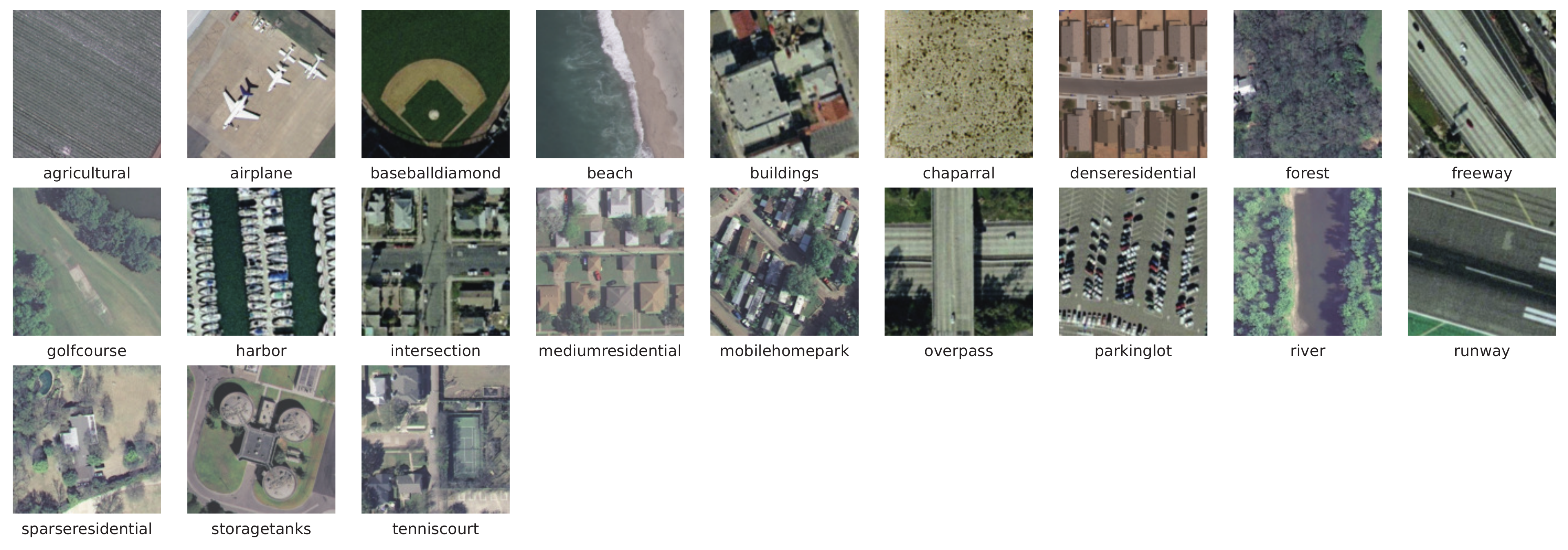
Remote sensing images are extremely different from conventional images due to their unique capture methods. On the one hand, remote sensing images often have the characteristics of broad independent coverage, high resolution, and complex components, which causes difficulties in scene classification [1]. As shown in Figure 1a, each image contains multiple ground objects. On the other hand, scene images of different categories may have high similarities. Such “dense residential” and “medium residential” areas, as shown in Figure 1b, have the same components; the distribution of densities causes them to be slightly different. Extracting discriminative features is the key to solving such problems. How to enhance the local semantic representation capability and extract more discriminative features for aerial scenes remains to be investigated [19]. Another critical challenge for scene classification is the lack of data due to the difficulty of dataset labelling and the limitation of sensor characteristics [1]. Although a series of new datasets have been made public recently, the number of images and object categories are still relatively small compared with the natural scene dataset. Mining more supervision information becomes a way to solve such problems.

Figure 1. The challenges in RSISC: (a) complex spatial arrangement, and the coexistence of multiple ground objects; (b) high interclass similarity. The images are from the UC Merced Land-Use dataset [20] and the NWPU-RESISC45 dataset [2].

When the number of training samples is limited, acquiring more labels to supervise the network is an effective solution to alleviate the lack of data. We design a self-supervised branch that takes the feature maps of the backbone network as labels and uses self-supervised methods to process the feature maps of the backbone network as the input of the branch network, and the output of the branch network is used as the prediction result. Specifically, it includes a self-supervised block and a feature fusion block. The self-supervised block uses two methods to preprocess the feature maps. One is to shuffle the feature map after dividing the region. Noroozi et al. [21] argues that solving jigsaw puzzles can be used to teach a system that an object is made of parts and what these parts are. It is beneficial for the network to understand the relative position information between different image patches. The other is to mask the background region [15,22]. Remote sensing scene images often contain a large amount of background information, and background masking can mask redundant backgrounds and enhance the discriminative ability of the branch network. This is an efficient solution to address the challenge of discriminative feature extraction. Different from SKAL [22], we propose masking the background by dividing the patch. Subsequent experiments show that this masking method is relatively flexible.

We adopt a feature pyramid network (FPN) [23] structure as the feature fusion block. The FPN structure has been used extensively in remote sensing [24,25]. It adopts a top-down method to fuse feature maps from different stages, and high-level features play a guiding role for low-level features. However, low-level and mid-level features are also essential for improving the features extracted in deep layers from a coarse level to a fine level [26]. Thus, we add a bottom-up fusion process to the branch network. Different locations in the image should have different attention weights, and due to the inherent density advantage of the image, the adjacent regions tend to have similar attention weight. Motivated by this, we propose a feature fusion module; it dynamically weights the feature map by assigning different attention weights to the patches.

The large memory and computation cost of branch structure cannot be ignored, so we embed the knowledge distillation method in SSKDNet. Inspired by FRSKD [27] and BAKE [28], the branch labels are served as soft logits to distil knowledge to the backbone, and the backbone integrates sample-similarity-level soft logits to guide itself. We only adopt the backbone during inference to reduce the computational load.

The main contributions of this article are summarized as follows:

1.

The performance of the Cycle MLP [18] model in RSISC is explored, and the SSKDNet model is proposed, enhancing the discriminative ability of Cycle MLP through self-supervised learning and knowledge distillation.

2.

We propose a self-supervised learning branch to learn the backbone feature maps. It includes a self-supervised block and a feature fusion block. The self-supervised block masks background regions by an attention mechanism and shuffles the feature map after dividing the region to improve the discriminative ability of the branch. The feature fusion block dynamically weights the feature maps of different stages, enhancing the high-level features from a coarse level to a fine level.

3.

The backbone integrates the “dark knowledge” of the branch via knowledge distillation to reduce the computation of the inference. It ensembles the sample-similarity-level soft logits to guide itself, which fully uses the similarity information between samples. Moreover, SSKDNet dynamically weights multiple losses via a principled loss function [29] to reduce training costs.

The remainder of this article is organized as follows. Section 2 presents related work on RSISC, MLP, self-supervised learning and knowledge distillation. In Section 3, our proposed model is described in detail. In Section 4, the effectiveness of SSKDNet is demonstrated through experiments on three datasets. Section 5 discusses the advantages of our self-supervised branch. Section 6 provides the concluding remarks.

2. Related Work

2.1. Remote Sensing Image Scene Classification Methods

Early feature extraction methods in RSISC are mainly based on handcrafted feature extraction. Handcrafted feature-based methods always use some salient feature descriptors. Typical feature descriptors are scale-invariant feature transformation (SIFT) [30], color histogram (CH) [31], texture descriptors (TD) [32], and HOG [33]. These methods mainly extract low-level information from images. CH and TD can represent an entire image with features, so they can be directly applied for remote scene classification. However, SIFT and HOG cannot directly represent an entire image because of their local characteristics. In order to represent an entire image with local descriptors, SIFT and HOG are encoded by some encoding methods, such as a vector of locally aggregated descriptors [34] and bag-of-visual-words (BoVWs) [20]. These approaches rely heavily on manual design, and it is not easy for them to achieve satisfactory results.

With the development of artificial intelligence, deep learning methods have been widely used in RSISC [1]. Traditional deep learning methods include CNNs, generative adversarial networks (GANs), and graph convolutional networks (GCNs). For CNNs, Li et al. [35], Wu et al. [36], and Shi et al. [37] proposed an attention module to enhance the extraction ability of discriminative features; Shi et al. [38,39] designed a lightweight module to reduce model parameters; and Bi et al. [19] and Wang et al. [22] further improved the classification accuracy by a key area detection strategy. For GANs, Ma et al. [40] proposed a supervised progressive growing generative adversarial network and significantly improved the classification accuracy in the case of limited samples; Gu et al. [41] introduced a pseudo-labelled sample generation method to solve the geographic errors of generated pseudo-labelled; and Ma et al. [42] designed a framework with error-correcting boundaries and a feature adaptation metric. For GCNs, Xu et al. [43] introduced the use of graph convolution to effectively capture the potential context relationships of the scene images; Peng et al. [44] proposed a multi-output network combining GCNs and CNNs. Recently, some novel methods have also been applied to RSISC, such as the CapsNet [45], neural architecture search [46], meta learning [47], etc. Deep learning methods have become the mainstream natural image feature extraction method due to their powerful feature extraction capabilities. They can automatically learn the most discriminative semantic-level features from the raw images compared with handcrafted feature-based methods. Furthermore, CNN models are end-to-end trainable architectures rather than complex multi-stage architectures [22]. However, these methods ignore logits and potential natural labels. SSKDNet can effectively use this supervision information.

2.2. MLP

While CNNs have been the main model for computer vision [48], recently, the ViT [12] introduced transformers into computer vision and attained SOTA performance. The transformer architecture computes representations for each individual token in parallel and aggregates spatial information across tokens via a multi-head self-attention mechanism. It can effectively establish contextual information. Lv et al. [11] explored the performance of the ViT model in RSISC and proposed the SCViT model. Hao et al. [49] designed a two-stream swin transformer network for special processing of remote sensing images to make the network focus on the target object in the scene. However, the computational complexity of self-attention is proportional to the square of tokens. In a series of works, refs. [50,51] proposed a computational approach from local attention to global attention to improve this problem. At the same time, researchers began to consider whether the self-attention mechanism is necessary. Tolstikhin et al. [16] designed a mixed MLP to replace the self-attention mechanism and achieved better results than ViT. Tang et al. [17] further proposed a sparse MLP to reduce the computational complexity. Liu et al. [15] designed the spatial gating unit to enhance the information interaction of tokens, further improving the performance of MLP. However, the complexity of these methods is still quadratic with the size of the image. Recently, Chen et al. [18] proposed a Cycle MLP, which achieved linear computational complexity through the dynamic shift and achieved competitive results in object detection, strength segmentation, and semantic segmentation. In SSKDNet, Cycle MLP is used as the backbone network.

2.3. Self-Supervised Learning

Self-supervised learning of visual representations is a fast-growing subfield of unsupervised learning. In recent years, many methods have been proposed and applied. Doersch et al. [52] and Wang et al. [53] proposed to use the location information and pixel values of the images as supervised labels. Bert [54] applied mask language model training to the NLP domain. He et al. [55] further verified the effectiveness of this class of methods by applying self-supervised masks to the computer vision domain. In scene classification, Zhao et al. [56] introduced a multitask learning framework that combines the tasks of self-supervised learning and scene classification. Stojnic et al. [57] showed that for the downstream task of remote sensing images, using self-supervised pre-training on remote sensing images can give better results than supervised pre-training on images of natural scenes. These methods have achieved SOTA performance. However, in scene classification, the effectiveness of self-supervised learning remains to be further explored.

2.4. Knowledge Distillation

Knowledge distillation transfers knowledge from a cumbersome teacher model to a lightweight student model. The pioneering work [58] performs knowledge representation of a teacher model using the softmax output layer, which converts the probability into soft logits with a temperature parameter. Following this, many works proposed new approaches to knowledge distillation. Tung et al. [59] proposed that similar samples have pairwise activation similarities and supervised the student network by pairwise activation similarities of similar samples of the teacher network. Zagoruyko et al. [60] proposed an attention map distillation method. Ji et al. [27] utilized both feature map distillation and soft logit distillation.

Knowledge distillation is also used to improve the RSISC accuracy. The discriminative modality distillation approach was introduced in [61]. Xu et al. [14] proposed an end-to-end method by employing ViT as an excellent teacher for guiding small networks in RSISC. Zhao et al. [62] introduced a novel pair-wise similarity knowledge distillation method. Chen et al. [63] introduced a knowledge distillation framework, which makes the output of the student and teacher models match. Zhang et al. [64] proposed a novel noisy label distillation method. The self-distillation learning method has few relevant research works in RSISC. We propose an end-to-end network architecture that combines the self-supervised learning method and knowledge distillation.

3. Materials and Methods

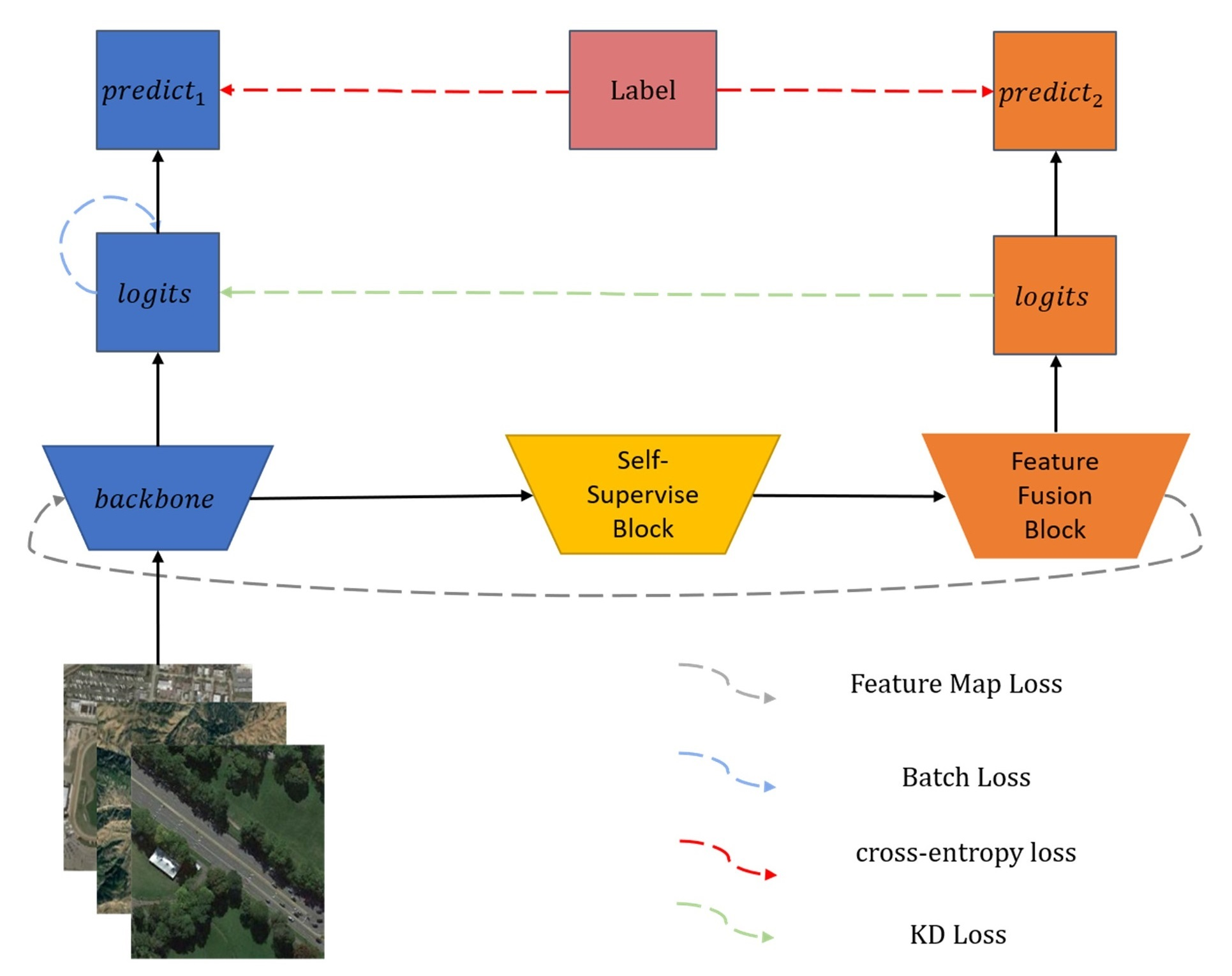
This section explains the specific details of the proposed SSKDNet for RSISC. The overall structure of the SSKDNet model is displayed in Figure 2. It consists of a backbone and a self-supervised branch. The backbone adopts Cycle MLP [18], and the self-supervised branch includes a self-supervised block and a feature fusion block. We present the backbone in Section 3.1, the self-supervised branch in Section 3.2, knowledge distillation in Section 3.3, and loss functions of SSKDNet in Section 3.4.

Figure 2. Structure of SSKDNet. The backbone feature maps ${\mathit{E}}_1$–${\mathit{E}}_5$ are the baseline structure Cycle MLP pre-trained on ImageNet; the feature maps ${\mathit{T}}_2$–${\mathit{T}}_5$ represent the output from the self-supervised block; the feature maps ${\mathit{M}}_5$–${\mathit{M}}_2$ represent the top-down path; and the feature maps ${\mathit{P}}_2$–${\mathit{P}}_5$ are the bottom-up path.

3.1. Backbone

Cycle MLP [18] is used as our backbone in the feature extraction stage. We denote stage1-stage5 as $f_1(.)$–$f_5(.)$. $f_1(.)$ represents patch embedding, which downsamples a quarter of the original input spatial dimension. $f_2(.)$–$f_5(.)$ stack 3, 4, 24, and 3 cycle fully connected (FC) layers (Section 3.1.1), respectively. The outputs have 96, 192, 384, and 768 channel dimensions, respectively. After each stage, the spatial dimension is downsampled by half. The feature maps of the backbone can be formulated as follows.

$${\mathit{E}}_{\mathrm{i}}=f_{\mathrm{i}}\left({\mathit{E}}_{\mathrm{i}-1}\right)$$

(1)

where ${\mathit{E}}_{\mathrm{i}}$ is the output feature map of $f_{\mathrm{i}}(.)$, and ${\mathit{E}}_{\mathrm{i}-1}$ is the feature map from the former layer. Specifically, the feature map ${\mathit{E}}_0$ is the input image. For the j-th sample, the predictive probability vector ${\mathit{predict}}_1$ can be obtained via a softmax function on the logits ${\mathit{z}}_{\mathrm{j}}=[z_{\mathrm{j}}^1,z_{\mathrm{j}}^2,\dots ,z_{\mathrm{j}}^M]\in {\mathbb{R}}^{1\times M}$, where M is the category number. The probability of class k can be formulated as follows.

$${\mathit{predict}}_1\left(k\right)=\frac{exp\left({\mathbf{z}}_{\mathrm{j}}^k\right)}{{\sum }_{\mathrm{i}=1}^{M}exp\left({\mathbf{z}}_{\mathrm{j}}^i\right)}$$

(2)

3.1.1. Cycle MLP

We denote the input feature map as $\mathit{X}\in {\mathbb{R}}^{H\times W\times C}$, where H, W, C are the height of the feature map, the width of the feature map and the number of channels. As shown in Figure 3a, channel FC allows communication between different channels, and it can handle various input scales. However, it cannot provide spatial information interactions. As shown in Figure 3b, spatial FC allows communication between different spatial locations. However, its computational complexity is quadratic with the image scale. As shown in Figure 3c, Cycle FC allows communication between channels and spatial locations by adding a shift operation, and it has linear complexity.

Figure 3. (a) Channel FC. (b) Spatial FC. (c) Cycle FC. (d) An example of Cycle FC. This image is quoted from [18] Notably, the index in Figure 3d has been modified to start from ${\delta }_i\left(0\right)$, and the last index is ${\delta }_i\left(8\right)$.

We use subscripts to index the feature map. For example, ${\mathit{X}}_{i,j,c}$ is the value of the c-th channel at the spatial position $(i,j)$, and ${\mathit{X}}_{i,j,:}$ are values of all channels at the spatial position $(i,j)$. The Cycle FC can be formulated as follows.

$$\mathrm{CycleFC}{\left(\mathit{X}\right)}_{i,j,:}=\sum _{c=0}^C{\mathit{X}}_{i+{\delta }_i\left(c\right),j+{\delta }_j\left(c\right),c}·{\mathit{W}}_{c,:}^{mlp}+\mathit{b}$$

(3)

$${\delta }_i\left(c\right)=\left(cmod{S}_H\right)-1,{\delta }_j\left(c\right)=(\lfloor \frac{C}{S_H}\rfloor mod{S}_W)-1$$

(4)

where $S_H$ and $S_W$ are $s\mathrm{t}epsizes$ along with the height and width dimensions, respectively. ${\delta }_i\left(c\right)$ and ${\delta }_j\left(c\right)$ are spatial offsets on the c-th channel. ${\mathbf{W}}^{mlp}\in {\mathbb{R}}^{C\times C_{ou\mathrm{t}}}$ and $\mathit{b}\in {\mathbb{R}}^{C_{ou\mathrm{t}}}$ are parameters of Cycle FC. Figure 3d shows the Cycle FC when $S_H=3$ and $S_W=1$.

3.2. Self-Supervised Branch

The self-supervised branch includes a self-supervised block and a feature fusion block. The self-supervised block is shown in Figure 4. This block performs patch embedding on the backbone feature maps ${\mathit{E}}_2$–${\mathit{E}}_5$, and then feeds the features into the gMLP [15] to extract local information ${\mathit{S}}_2$–${\mathit{S}}_5$. The final feature maps ${\mathit{T}}_2$–${\mathit{T}}_5$ are obtained by passing the adjacent ${\mathit{S}}_2$–${\mathit{S}}_5$ through a Cross MLP, which is an information interaction module. Notably, ${\mathit{E}}_2$–${\mathit{E}}_5$ are processed differently. ${\mathit{E}}_2$ masks a part of the background by background masking. ${\mathit{E}}_3$ shuffles the regions after dividing the regions by jigsaw puzzle. ${\mathit{E}}_4$ is fed directly into the gMLP after patch embedding. ${\mathit{E}}_5$ is utilized to calculate the attention map. The feature fusion block is shown at the bottom of Figure 2, which is achieved by a top-down and bottom-up bidirectional fusion. We use a feature fusion module to fuse adjacent feature maps and use the feature maps ${\mathit{P}}_2$–${\mathit{P}}_5$ as the self-supervised prediction results.

Figure 4. The self-supervised block. $H_{\mathrm{i}},W_{\mathrm{i}},p_{\mathrm{i}}$ are the height, width and patch size of the feature map ${\mathit{E}}_{\mathrm{i}}$, respectively.

3.2.1. Background Masking

Masking background regions is an effective way to extract discriminative features [22]. As shown in Figure 4a,d, we calculate the attention map of the high-level feature map ${\mathit{E}}_5$. The attention map $\mathit{attn}$ for each position $(i,j)$ is calculated as follows.

$${\mathit{attn}}_{\mathrm{i},\mathrm{j}}=\frac{1}{C}\sum _{\mathrm{k}=1}^C{\mathit{E}}_{5,\mathrm{i},\mathrm{j},\mathrm{k}}$$

(5)

where ${\mathit{E}}_{5,\mathrm{i},\mathrm{j},\mathrm{k}}$ is the element of ${\mathit{E}}_5$, and C is the number of channels of ${\mathit{E}}_5$. We upsample the attention map $\mathit{attn}$ to the same spatial shape as ${\mathit{E}}_2$ by the nearest interpolation, record the positions of $75\%$ of feature points with the lowest attention weights, and then delete the corresponding tokens in the feature map ${\mathit{E}}_2$. We pad a vector $\mathbf{1}$ with an initial value of 1 to replace the deleted tokens. It is well known that high-level feature maps contain high-level semantic information, and the network tends to pay more attention to points with higher activation values. Thus, the channel means of the feature map ${\mathit{E}}_5$ can effectively calculate the attention map of the network. Later experiments can also verify this.

3.2.2. Jigsaw Puzzle

We expect SSKDNet to learn more location information about images. Noroozi et al. [21] proposed to divide the feature map into different regions, erase the edge information and randomly shuffle the regions. As shown in Figure 4b, we adopt a similar method to divide the feature map into four regions, erase the edge information of the feature map, and then shuffle them randomly.

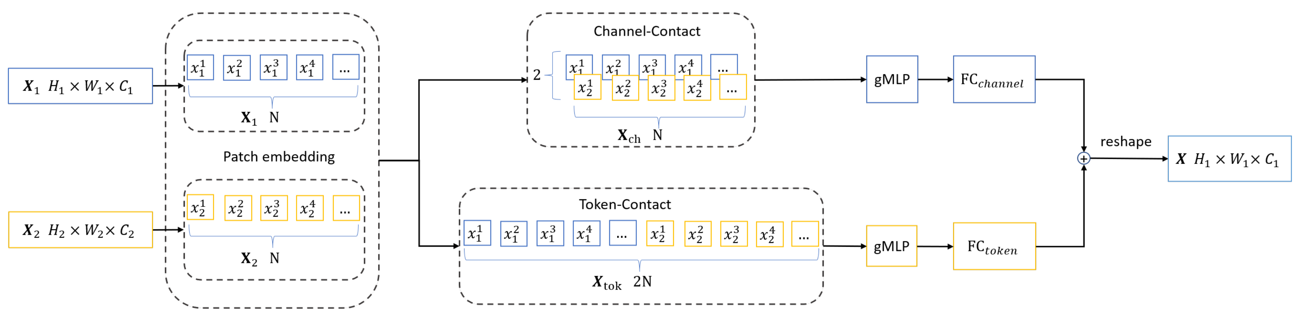
3.2.3. Cross MLP

Compared with convolution and transformer, gMLP [15] alternately constructs FC layers along the channel dimension and the token dimension, which can extract global features easily. As shown in Figure 5, we propose a Cross MLP module to obtain more complete semantic information from adjacent feature maps. The Cross MLP has two parallel gMLP with a larger receptive field. It can be formulated as follows.

$$\begin{array}{cc}\hfill {\mathit{X}}_{\mathrm{ch}}& =Conca\mathrm{t}(P_{emb}\left({\mathit{X}}_1\right),P_{emb}\left({\mathit{X}}_2\right),dim=channel)\hfill \\ \hfill {\mathit{X}}_{\mathrm{tok}}& =Conca\mathrm{t}(P_{emb}\left({\mathit{X}}_1\right),P_{emb}\left({\mathit{X}}_2\right),dim=token)\hfill \\ \mathrm{Cross}\mathrm{MLP}({\mathit{X}}_1,{\mathit{X}}_2)\hfill & =F{C}_{channel}\left(gMLP\left({\mathit{X}}_{ch}\right)\right)+F{C}_{\mathrm{t}oken}\left(\mathrm{gMLP}\left({\mathit{X}}_{\mathrm{tok}}\right)\right))\hfill \end{array}$$

(6)

where ${\mathit{X}}_1\in {\mathbb{R}}^{H_1\times W_1\times C_1}$ and ${\mathit{X}}_2\in {\mathbb{R}}^{H_2\times W_2\times C_2}$ are the input feature maps. $P_{emb}(.)$ represents patch embedding with $patchsize=1$. $P_{emb}\left({\mathit{X}}_1\right)$ and $P_{emb}\left({\mathit{X}}_2\right)$ are split tokens, $P_{emb}\left({\mathit{X}}_1\right)={[{\mathit{x}}_1^1,{\mathit{x}}_1^2,\dots ,{\mathit{x}}_1^{\mathrm{N}}]}^{\mathrm{t}}$, $P_{emb}\left({\mathit{X}}_2\right)={[{\mathit{x}}_2^1,{\mathit{x}}_2^2,\dots ,{\mathit{x}}_2^{\mathrm{N}}]}^{\mathrm{t}}$, where N is the number of tokens. We concatenate $P_{emb}\left({\mathit{X}}_1\right)$ and $P_{emb}\left({\mathit{X}}_2\right)$ along the channel dimension and token dimension to obtain ${\mathit{X}}_{\mathrm{ch}}$ and ${\mathit{X}}_{\mathrm{tok}}$ by $Concat$, respectively. gMLP [15] is used for information interaction between channels and tokens, and $F{C}_{channel}$ and $F{C}_{\mathrm{t}oken}$ are FC layers along the channel dimension and token dimension to adjust the size of ${\mathit{X}}_{\mathrm{ch}}$ and ${\mathit{X}}_{\mathrm{tok}}$, respectively.

Figure 5. The Cross MLP module.

As shown in Figure 4, the feature maps ${\mathbf{S}}_2$–${\mathbf{S}}_5$ are the input. We can obtain the self-supervised block output ${\mathit{T}}_2$–${\mathit{T}}_5$ from the following formula.

$${\mathit{T}}_{\mathrm{t}}=\left\{\begin{array}{cc}Conv\left(upsample({\mathit{S}}_{\mathrm{t}}+\mathrm{CrossMLP}({\mathit{S}}_{\mathrm{t}},{\mathit{S}}_{\mathrm{t}+1}))\right),\hfill & \mathrm{t}=2\hfill \\ Conv\left(upsample({\mathit{S}}_{\mathrm{t}}+\mathrm{CrossMLP}({\mathit{S}}_{\mathrm{t}},{\mathit{S}}_{\mathrm{t}-1})+\mathrm{CrossMLP}({\mathit{S}}_{\mathrm{t}},{\mathit{S}}_{\mathrm{t}+1}))\right),\hfill & \mathrm{t}=3\hfill \\ Conv\left(upsample({\mathit{S}}_{\mathrm{t}}+\mathrm{CrossMLP}({\mathit{S}}_{\mathrm{t}},{\mathit{S}}_{\mathrm{t}-1})+\mathrm{CrossMLP}({\mathit{S}}_{\mathrm{t}},upsample\left({\mathit{S}}_{\mathrm{t}+1}\right)))\right),\hfill & \mathrm{t}=4\hfill \\ Conv\left(upsample({\mathit{S}}_{\mathrm{t}}+\mathrm{CrossMLP}({\mathit{S}}_{\mathrm{t}},downsample\left({\mathit{S}}_{\mathrm{t}-1}\right)))\right),\hfill & \mathrm{t}=5\hfill \end{array}\right.$$

(7)

Before Cross MLP, the feature maps ${\mathbf{S}}_{\mathrm{t}-1}$ and ${\mathbf{S}}_{\mathrm{t}+1}$ are adjusted to be the same as the spatial size of the ${\mathbf{S}}_{\mathrm{t}}$ by upsample or downsample. The upsample adopts nearest interpolation, and the downsample adopts convolution with kernel size $(2\times 2)$ and stride = 2, where $Conv(·)$ denotes a $1\times 1$ convolutional layer. We adjust the output ${\mathit{T}}_2$–${\mathit{T}}_5$ to the same size as ${\mathit{E}}_2$–${\mathit{E}}_5$ by upsample and $Conv(·)$.

As shown in Table 1, we show the parameter settings for patch embedding in the self-supervised block, where $p_{\mathrm{i}}$ and $c_{\mathrm{i}}$ are patch size and the number of channels, respectively, and (a)–(d) correspond to the different branchs of Figure 4.

Table 1. The parameter settings in the self-supervised block.

Branch	Input Size	Patch Embedding	Middle Output Size	Output Size
(a)	${\mathit{E}}_2(64\times 64\times 96)$	$p_2=4,c_2=96$	${\mathit{S}}_2(16\times 16\times 96)$	${\mathit{T}}_2(64\times 64\times 96)$
(b)	${\mathit{E}}_3(32\times 32\times 192)$	$p_3=2,c_3=96$	${\mathit{S}}_3(16\times 16\times 96)$	${\mathit{T}}_3(32\times 32\times 192)$
(c)	${\mathit{E}}_4(16\times 16\times 384)$	$p_4=1,c_4=96$	${\mathit{S}}_4(16\times 16\times 96)$	${\mathit{T}}_4(16\times 16\times 384)$
(d)	${\mathit{E}}_5(8\times 8\times 768)$	$p_5=1,c_5=96$	${\mathit{S}}_5(8\times 8\times 96)$	${\mathit{T}}_5(8\times 8\times 768)$

3.2.4. Feature Fusion Block

We dynamically weight adjacent feature maps by setting a weight for each patch of the feature map. As shown in Figure 6, for the input ${\mathit{X}}_1\in {\mathbb{R}}^{H_1\times W_1\times C_1}$ and ${\mathit{X}}_2\in {\mathbb{R}}^{H_2\times W_2\times C_2}$, the feature fusion module can be formulated as follows.

$$\mathit{X}=Fusion({\mathit{X}}_1,{\mathit{X}}_2)=P_{emb}\left({\mathit{X}}_1\right)·{\mathit{W}}_1+P_{emb}\left(upsample\left(Conv\left({\mathit{X}}_2\right)\right)\right)·{\mathit{W}}_2$$

(8)

where $Conv(·)$ denotes a $3\times 3$ convolutional layer, and $upsample$ is the nearest interpolation. We adjust ${\mathit{X}}_2$ to the same spatial and channel shape as ${\mathit{X}}_1$ by $Conv$ and $upsample$ (when the spatial size of ${\mathit{X}}_2$ is greater than ${\mathit{X}}_1$, replace the $upsample$ with the $downsample$). Then the feature maps ${\mathit{X}}_1$ and ${\mathit{X}}_2$ are split into fixed-size tokens by $P_{emb}(.)$. $P_{emb}\left({\mathit{X}}_1\right)={[{\mathit{x}}_1^1,{\mathit{x}}_1^2,\dots ,{\mathit{x}}_1^{\mathrm{N}}]}^{\mathit{T}}$, and $P_{emb}\left({\mathit{X}}_2\right)={[{\mathit{x}}_2^1,{\mathit{x}}_2^2,\dots ,{\mathit{x}}_2^{\mathrm{N}}]}^{\mathit{T}}$, where N is the number of tokens. $\mathit{X}={[{\mathit{x}}^1,{\mathit{x}}^2,\dots ,{\mathit{x}}^{\mathrm{N}}]}^{\mathrm{t}}$ is the feature map after fusion of ${\mathit{X}}_1$ and ${\mathit{X}}_2$. We adjust the weight of the tokens by setting a pair of learnable vectors ${\mathit{W}}_{\mathbf{1}}={[w_1^1,w_1^2,\dots ,w_1^{\mathrm{N}}]}^{\mathrm{t}}$ and ${\mathit{W}}_{\mathbf{2}}={[w_2^1,w_2^2,\dots ,w_2^{\mathrm{N}}]}^{\mathrm{t}}$. Specifically, the j-th token ${\mathit{X}}^j$ is calculated as follows.

$${\mathit{x}}^{\mathrm{j}}={\mathit{x}}_1^{\mathrm{j}}\times w_1^{\mathrm{j}}+{\mathit{x}}_2^{\mathrm{j}}\times w_2^{\mathrm{j}}$$

(9)

Figure 6. The feature fusion module.

Dividing the feature map into patches allows the network to flexibly assign different attention weights to patches.

The top-down feature maps ${\mathit{M}}_2-{\mathit{M}}_5$ can be formulated as follows.

$${\mathit{M}}_{\mathrm{t}}=\left\{\begin{array}{cc}\hfill upsample\left(Conv\left({\mathit{T}}_{\mathrm{t}}\right)\right),\hfill & \mathrm{t}=5\hfill \\ Fusion({\mathit{T}}_{\mathrm{t}},{\mathit{M}}_{\mathrm{t}+1}),\hfill & \hfill \mathrm{t}=2,3,4\hfill \end{array}\right.$$

(10)

Similarly, the bottom-up feature maps ${\mathit{P}}_2-{\mathit{P}}_5$ can be formulated as follows.

$${\mathit{P}}_{\mathrm{t}}=\left\{\begin{array}{cc}\hfill downsample(Conv\left({\mathit{M}}_{\mathrm{t}}\right),\hfill & \hfill \mathrm{t}=2\hfill \\ \hfill Fusion({\mathit{M}}_{\mathrm{t}},{\mathit{P}}_{\mathrm{t}-1}),\hfill & \hfill \mathrm{t}=3,4,5\hfill \end{array}\right.$$

(11)

The difference between ${\mathit{M}}_i$ and ${\mathit{P}}_i$ is that upsample is substituted by downsample, and the downsample adopts convolution with kernel size $(2\times 2)$ and stride = 2.

For the setting of parameters $w_1^{\mathrm{j}}$ and $w_2^{\mathrm{j}}$, we initialize $w_1^{\mathrm{j}}$ and $w_2^{\mathrm{j}}$ to 1 and normalize them by the softmax function. It can be formulated as follows.

$$w_{\mathrm{i}}^{\mathrm{j}}=\frac{exp\left(w_{\mathrm{i}}^{\mathrm{j}}\right)}{{\sum }_{\mathrm{k}}exp\left(w_{\mathrm{k}}^{\mathrm{j}}\right)},\forall \mathrm{i}\in \left\{1,2\right\}$$

(12)

The weights are normalized to the range 0 to 1 by softmax to represent the importance of each input, which is an efficient attention calculation method. In the feature fusion block, we set the patch size of the patch embedding to 6, 8, and 16 in the top-down approach and set the patch size to 8, 4, and 2 in the bottom-up approach, respectively. The other settings are the same as FRSKD [27].

3.2.5. Feature Map Loss

For the backbone feature map ${\mathit{E}}_{\mathrm{t}}\in {\mathbb{R}}^{H\times W\times C}$, we denote ${\mathit{E}}_{\mathrm{t}}^{\prime }\in {\mathbb{R}}^{H\times W\times 1}$ as the channel mean of ${\mathit{E}}_{\mathrm{t}}$. $e_{\mathrm{avg}}$ and $e_{\mathrm{std}}$ are the mean and variance of ${\mathit{E}}_{\mathrm{t}}^{\prime }$, respectively. The normalization process can be formulated as follows.

$${\mathit{E}}_{\mathrm{t},\mathrm{i},\mathrm{j}}^{\prime }=({\mathit{E}}_{\mathrm{t},\mathrm{i},\mathrm{j}}^{\prime }-e_{\mathrm{avg}})/e_{\mathrm{std}}$$

(13)

Similarly, for the branch feature map ${\mathit{P}}_{\mathrm{t}}$, we can calculate the normalized feature map ${\mathit{P}}_{\mathrm{t}}^{\prime }$. The feature map loss can be formulated as follows.

$$L_{em}^{FM}=\sum _{\mathrm{t}=2}^5\sum _{\mathrm{i}=1}^{\mathrm{H}}\sum _{\mathrm{j}=1}^{\mathrm{W}}{({\mathit{E}}_{\mathrm{t},\mathrm{i},\mathrm{j}}^{\prime }-{\mathit{P}}_{\mathrm{t},\mathrm{i},\mathrm{j}}^{\prime })}^2$$

(14)

The gradients through ${\mathit{E}}_{\mathrm{t},\mathrm{i},\mathrm{j}}^{\prime }$ are not propagated to avoid the model collapse issue.

3.3. Knowledge Distillation

Knowledge distillation can be viewed as normalizing the training of the student network with soft targets that carry the “dark knowledge” of the teacher network. We combine two knowledge distillation methods so that the backbone can obtain knowledge from the branch and itself. The knowledge distillation methods include soft logit distillation and batch distillation.

We denote $\mathit{Z}=[{\mathit{z}}_1,{\mathit{z}}_2,\dots ,{\mathit{z}}_N]\in {\mathbb{R}}^{N\times M}$ as the logit vectors of the backbone in the same batch. For the j-th sample, the backbone logit vector ${\mathit{z}}_{\mathrm{j}}=[z_{\mathrm{j}}^1,z_{\mathrm{j}}^2,\dots ,z_{\mathrm{j}}^M]\in {\mathbb{R}}^{1\times M}$, where M is the number of categories, and N is the number of samples in a batch.

3.3.1. Soft Logits Distillation

The soft logit output by the network contains more information about sample than just the class label. For the j-th sample, the backbone soft logits ${\mathit{P}}_j^{\tau }\in {\mathbb{R}}^{1\times M}$ can be obtained by a softmax function, and the soft logits of the k-th class can be formulated as follows.

$${\mathit{p}}_{\mathrm{j}}^{\tau }\left(\mathrm{k}\right)=\frac{exp(z_{\mathrm{j}}^{\mathrm{k}}/\tau )}{{\sum }_{\mathrm{i}=1}^{M}exp(z_j^i/\tau )}$$

(15)

The $\tau$ is the temperature hyper-parameter which is used to soften the logits. Similarly, we can obtain the branch soft logits ${\mathbf{q}}_j^{\tau }\in {\mathbb{R}}^{1\times M}$. The Kullback–Leibler (KL) loss is used to measure the similarity of two distributions. The KL loss can be formulated as follows.

$$L_{logi\mathrm{t}s}^{KL}=L^{KL}({\mathit{q}}_{\mathrm{j}}^{\tau }\Vert {\mathit{p}}_{\mathrm{j}}^{\tau })=\sum _{\mathrm{i}=1}^M{\mathit{q}}_{\mathrm{j}}^{\tau }\left({\mathit{x}}_{\mathrm{i}}\right)log\frac{{\mathit{q}}_{\mathrm{j}}^{\tau }\left({\mathit{x}}_{\mathrm{i}}\right)}{{\mathit{p}}_{\mathrm{j}}^{\tau }\left({\mathit{x}}_{\mathrm{i}}\right)}$$

(16)

3.3.2. Batch Distillation

Samples with high visual similarities are expected to make more consistent predictions about their predicted class probabilities, regardless of these truth labels. In this part, the batch knowledge ensembling (BAKE) [28] is introduced to obtain excellent soft logits. It achieves knowledge ensembling by aggregating the “dark knowledge” from different samples in the same batch. We can obtain the pairwise similarity matrix $\mathit{A}\in {\mathbb{R}}^{N\times N}$ by the dot product of the logits. ${\mathit{A}}_{\mathrm{i},\mathrm{j}}$ represents the affinity between the samples with indexes i and j, and it can be formulated as follows.

$${\mathit{A}}_{\mathrm{i},\mathrm{j}}=\sigma {\left({\mathbf{z}}_{\mathrm{i}}\right)}^{{T}}\sigma \left({\mathbf{z}}_{\mathrm{j}}\right)$$

(17)

where $\sigma \left(\mathit{f}\right)=\mathit{f}/{\parallel \mathit{f}\parallel }_2$. We normalize each row of the affinity matrix $\mathit{A}$ to obtain $\widehat{\mathit{A}}$,

$${\widehat{\mathit{A}}}_{\mathrm{i},\mathrm{j}}=\frac{exp\left({\mathit{A}}_{\mathrm{i},\mathrm{j}}\right)}{{\sum }_{\mathrm{i}\ne \mathrm{j}}exp\left({\mathit{A}}_{\mathrm{i},\mathrm{j}}\right)},\forall \mathrm{i}\in \left\{1,2\dots N\right\}$$

(18)

For the i-th sample, the soft logits ${\mathit{p}}_j^{\tau }\in {\mathbb{R}}^{1\times M}$, we denote the soft logits of samples within the same batch as ${\mathit{P}}^{\tau }={[{\mathit{p}}_1^{\tau },\dots ,{\mathit{p}}_N^{\tau }]}^{\mathrm{t}}\in {\mathbb{R}}^{N\times M}$. Based on Equations (17) and (18), we can obtain the soft logits ${\mathit{Q}}^{\tau }={[{\mathbf{q}}_1^{\tau },\dots ,{\mathbf{q}}_N^{\tau }]}^{\mathit{T}}\in {\mathbb{R}}^{N\times M}$ aggregated from the sample information,

$${\mathit{Q}}^{\tau }=(1-\omega ){(I-\omega \widehat{\mathit{A}})}^{-1}{\mathit{P}}^{\tau }$$

(19)

where $\omega \in [0,1]$ is the weighting factor. For the j-th sample, the batch KL loss can be formulated as follows.

$$L_{ba\mathrm{t}ch}^{KL}=L^{KL}({\mathit{q}}_{\mathrm{j}}^{\tau }\Vert {\mathit{p}}_{\mathrm{j}}^{\tau })=\sum _{\mathrm{i}=1}^M{\mathit{q}}_{\mathrm{j}}^{\tau }\left(x_{\mathrm{i}}\right)log\frac{{\mathit{q}}_{\mathrm{j}}^{\tau }\left(x_{\mathrm{i}}\right)}{{\mathit{p}}_j^{\tau }\left(x_i\right)}$$

(20)

Notably, in Equation (20), ${\mathit{q}}_{\mathrm{j}}^{\tau }$ is different from Equation (16). The parameters for knowledge distillation are set the same as in BAKE [28].

3.4. Loss Function of SSKDNet

The SSKDNet is optimized by minimizing the loss function. Our loss function consists of three parts, including knowledge distillation loss (Equations (16) and (20)), cross-entropy loss (Equations (22) and (23)), and feature map loss (Equation (14)). The total loss can be formulated as follows.

$$L_{\mathrm{t}o\mathrm{t}al}={\alpha }_1\times L_{logi\mathrm{t}s}^{KL}+{\alpha }_2\times L_{ba\mathrm{t}ch}^{KL}+{\alpha }_3\times L_{c{e}_1}+{\alpha }_4\times L_{c{e}_2}+{\alpha }_5\times L_{em}^{FM}$$

(21)

$$L_{c{e}_1}=-\sum _{k=1}^M(y_k\times log\left({\mathit{predict}}_1\left(k\right)\right))$$

(22)

$$L_{c{e}_2}=-\sum _{k=1}^M(y_k\times log\left({\mathit{predict}}_2\left(k\right)\right))$$

(23)

where ${\mathit{predict}}_1$ and ${\mathit{predict}}_2$ are the backbone and branch predictions, respectively. $L_{c{e}_1}$ and $L_{c{e}_2}$ represent the cross-entropy loss functions from the backbone and self-supervised branch. ${\alpha }_1,{\alpha }_2,{\alpha }_3,{\alpha }_4,$ and ${\alpha }_5$ are the weight coefficients. We introduce a multi-task loss function [29] to reduce the extra cost of hyperparameters. Specifically, we set the weight coefficients as learnable variables and optimize them using the following formula.

$$L_{\mathrm{t}o\mathrm{t}al}=\frac{1}{2{{\alpha }_1}^2}{L}_{logi\mathrm{t}s}^{KL}+\frac{1}{2{{\alpha }_2}^2}{L}_{ba\mathrm{t}ch}^{KL}+\frac{1}{2{{\alpha }_3}^2}{L}_{c{e}_1}+\frac{1}{2{{\alpha }_4}^2}{L}_{c{e}_2}+\frac{1}{2{{\alpha }_5}^2}{L}_{em}^{FM}+\sum _{i=1}^{5}log\left({\alpha }_i\right)$$

(24)

where ${\alpha }_1,{\alpha }_2,{\alpha }_3,{\alpha }_4,$ and ${\alpha }_5$ are learnable parameters. This loss function is smoothly differentiable and is well-formed such that the task weights do not converge to zero. In contrast, directly learning the weights using a simple linear sum of losses would result in weights that quickly converge to zero.

4. Results

In this section, we conduct comprehensive experiments and analyses on three public scene classification datasets. We first introduce these datasets, evaluation metrics and experimental settings. Then, we compare the performance differences between our method and several SOTA methods. Finally, we perform ablation experiments for each module.

4.1. Datasets

To verify the effectiveness of SSKDNet, we used three commonly used datasets, including the UC Merced Land-Use (UCM) dataset [20], the Aerial Image (AID) dataset [2], and the NWPU-RESISC45 (NWPU) dataset [65].

(1)

The UCM dataset is one of the oldest datasets in the RSISC domain. It has 21 classes (“harbour”, “intersection”, “overpass”, “chaparral”, etc.) and 1000 images per category extracted from the United States Geological Survey National Map, Urban Area Imagery collection. The size of each image is $256\times 256$ pixels. Some sample examples are shown in Figure 7.

Figure 7. Some samples from the UCM dataset.

(2)

The AID dataset is a high-spatial-resolution dataset for aerial scene classification, which has a size of 600 × 600 pixels. It has 30 classes (“church”, “medium residential”, “storage tanks”, “port”, “playground”, etc.). All images are extracted from Google Earth Imagery. Some sample examples are shown in Figure 8.

Figure 8. Some samples from the AID dataset.

(3)

The NWPU dataset contains 45 scene classes (“lakes”, “beach”, “church”, “desert”, “freeway”, etc.) with 700 images in each class, and the size of each image is 256 × 256 pixels. Some sample examples are shown in Figure 9.

Figure 9. Some samples from the NWPU dataset.

4.2. Evaluation Metrics

The overall accuracy (OA) and confusion matrix were used as the primary quantitative measures. OA is the proportion of the number of correctly predicted samples in the total data, which reflects the overall performance of the classification. The confusion matrix is a two-dimensional table that analyses the between-class classification errors and confusion degree. Rows and columns represent all samples of a predicted class and samples of a true class, respectively.

We randomly split datasets using the same training ratio, repeated the experiment five times, and reported the mean and standard deviation.

4.3. Experimental Setup

We followed the conventional settings. A total of $80\%$ of images from the UCM dataset were randomly selected for training, and the remainder data were used for evaluation. Similarly, we randomly selected $20\%$ and $50\%$ of the images from AID for training and $10\%$ and $20\%$ of the images of NWPU for training. During training, the image size was set to 256 × 256. The image augmentation methods included random horizontal flipping, random resized cropping and random erasing. All models were trained for 60 epochs, with a batch size set to 50 and AdamW (with a weight decay of 0.05) [66] chosen as optimizer. The initial learning rate was set to 0.0001, divided by 10 every 30 epochs. We used an RTX3090 GPU in all experiments. The implementation was based on Python 3.8 with Pytorch.

4.4. Comparison with Other Methods

This subsection describes the experimental results on the three remote sensing scene image datasets in detail. We divided the compared methods into two categories: classic CNNs-based methods, including GoogLeNet [2], VGG-VD-16 [2], SCCov [67], ResNet50 [68], ResNet-50+EAM [68], LCNN-BFF [69], BiMobileNet [70], DFAGCN [43], and MF${}^2$CNet [71], and ViT-based methods, including Fine-tune ViT [11] and ET-GSNet [14]. The backbone Cycle MLP [18] was also included for comparison.

Table 2 shows the comparison results on the UCM dataset. Since there are only 420 test images in this dataset, many current methods can easily achieve more than 99% accuracy. The classification accuracy tends to be saturated. Compared with other algorithms, our method achieves a higher accuracy of 99.62%, with an improvement of 0.1%. The confusion matrix on the UCM dataset is shown in Figure 10. Only one image in $mediumresidential$ is misclassified as $tenniscourts$, while other classes can achieve 100% accuracy.

Table 2. The comparison of OA on the UCM Dataset.

Method	Year	80% Training Ratio
GoogLeNet [2]	2017	$94.31\pm 0.89$
VGG-VD-16 [2]	2017	$95.21\pm 1.20$
SCCov [67]	2019	$99.05\pm 0.25$
ResNet50 [68]	2020	$98.69\pm 0.49$
ResNet-50+EAM [68]	2020	$98.98\pm 0.37$
LCNN-BFF [69]	2020	$99.29\pm 0.24$
BiMobileNet [70]	2020	$99.03\pm 0.28$
DFAGCN [43]	2021	$98.48\pm 0.42$
MF${}^2$CNet [71]	2022	$99.52\pm 0.25$
Fine-tune ViT [11]	2020	$99.01\pm 0.21$
ET-GSNet [14]	2022	$99.29\pm 0.34$
Cycle MLP [18]	2022	$99.05\pm 0.39$
Ours	2022	$99.62\pm 0.10$

Figure 10. Confusion matrix on the UCM dataset under the training ratio of 80%.

Table 3 shows the results on the AID dataset. It can be seen that when the training ratios were 20% and 50%, our method achieved the best performance of 95.96% and 97.45%, respectively. Compared with other algorithms, the average OAs are improved by 0.38% and 0.27%, respectively. The confusion matrix on the AID dataset is shown in Figure 11, in which 29 categories can achieve more than 99% accuracy. The most confusing categories are $park$ and $square$. It can be seen in Figure 8 that the $park$ and $square$ categories have few distinct features, which makes them difficult to classify.

Table 3. The comparison of OA on the AID Dataset.

Method	Year	20% Training Ratio	50% Training Ratio
GoogLeNet [2]	2017	$83.44\pm 0.40$	$86.39\pm 0.55$
VGG-VD-16 [2]	2017	$86.59\pm 0.29$	$89.64\pm 0.36$
SCCov [67]	2019	$93.12\pm 0.25$	$96.10\pm 0.16$
ResNet50 [68]	2020	$92.57\pm 0.17$	$95.96\pm 0.17$
ResNet-50+EAM [68]	2020	$93.64\pm 0.25$	$96.62\pm 0.13$
LCNN-BFF [69]	2020	$91.66\pm 0.48$	$94.62\pm 0.16$
BiMobileNet [70]	2020	$94.83\pm 0.24$	$96.87\pm 0.23$
DFAGCN [43]	2021	−	$94.88\pm 0.22$
MF${}^2$CNet [71]	2022	$95.54\pm 0.17$	$97.02\pm 0.28$
Fine-tune ViT [11]	2020	$94.90\pm 0.29$	$96.49\pm 0.18$
ET-GSNet [14]	2022	$95.58\pm 0.18$	$96.88\pm 0.19$
Cycle MLP [18]	2022	$95.31\pm 0.15$	$97.18\pm 0.17$
Ours	2022	$95.96\pm 0.12$	$97.45\pm 0.19$

Figure 11. Confusion matrix on the AID dataset under the training ratio of 50%.

Table 4 presents the performance of our algorithm on the NWPU dataset. When the training ratios were 10% and 20%, we achieved results of 92.77% and 94.92%, which are 0.05% and 0.42% higher than the previous best method, respectively. The confusion matrix of the NWPU dataset is shown in Figure 12. Only two categories are lower than 90% accuracy, $palace$ and $church$. These two categories are relatively complex.

Table 4. The comparison of OA on the NWPU Dataset.

Method	Year	10% Training Ratio	20% Training Ratio
GoogLeNet [65]	2017	$82.57\pm 0.12$	$86.02\pm 0.18$
VGG-VD-16 [65]	2017	$87.15\pm 0.45$	$90.36\pm 0.18$
SCCov [67]	2019	$89.30\pm 0.35$	$92.10\pm 0.25$
ResNet50 [68]	2020	$88.48\pm 0.21$	$91.86\pm 0.19$
ResNet-50+EAM [68]	2020	$90.87\pm 0.15$	$93.51\pm 0.12$
LCNN-BFF [69]	2020	$86.53\pm 0.15$	$91.73\pm 0.17$
BiMobileNet [70]	2020	$92.06\pm 0.14$	$94.08\pm 0.11$
DFAGCN [43]	2021	−	$89.29\pm 0.28$
MF${}^2$CNet [71]	2022	$92.07\pm 0.22$	$93.85\pm 0.27$
Fine-tune ViT [11]	2020	$91.59\pm 0.19$	$93.90\pm 0.20$
ET-GSNet [14]	2022	$92.72\pm 0.28$	$94.50\pm 0.18$
Cycle MLP [18]	2022	$91.84\pm 0.17$	$94.27\pm 0.11$
Ours	2022	$92.77\pm 0.05$	$94.92\pm 0.12$

Figure 12. Confusion matrix on the NWPU dataset under the training ratio of 20%.

The computation costs (FLOPs) and parameters of the methods GoogLeNet [2], VGG-VD-16 [2], ResNet50 [68], Fine-tune ViT [11], BiMobileNet [70], MF${}^2$CNet [71] and Cycle MLP [18] are compared with our model. As shown in Table 5, SSKDNet has slightly more parameters than some baseline models, but we achieve higher accuracy. For instance, when compared with ResNet50 [68] on the AID dataset, we have an improvement of $3.41\%$. We only use the backbone during inference, so the inference speed of SSKDNet is same as Cycle MLP [18]. Compared with the ViT [11], we have a $1.08\%$ improvement at lower FLOPs and parameters.

Table 5. Comparison of computational costs and parameters on the AID dataset.

Methods	FLOPs	Parameters	20% Training Ratio
GoogLeNet [2]	1.97 G	6.62 M	83.44
VGG-VD-16 [2]	20.19 G	15.75 M	86.59
ResNet50 [68]	5.37 G	25.56 M	92.57
Fine-tune ViT [11]	21.98 G	86.38 M	94.90
BiMobileNet [70]	0.45 G	29.59 M	94.83
MF${}^2$CNet [71]	2.42 G	33.20 M	95.54
Cycle MLP [18]	13.41 G	63.96 M	95.31
Ours	16.14 G	77.15 M	95.98

4.5. Ablation Experiments

We validated the effectiveness of our module through ablation experiments. For each experiment, we set the same parameters and removed only one module at a time. Experiment 1 removed the background masking module and the jigsaw puzzle module in Figure 4. Experiment 2 removed the Cross MLP module in Figure 4. Experiment 3 removed the feature fusion module. Table 6 shows the performance on the AID dataset. When the background masking module and the jigsaw puzzle module are removed, the classification accuracy drops by 0.19%. When the Cross MLP module is removed, the classification accuracy drops by 0.16%. When the feature fusion module is removed, the accuracy drops by 0.1%. These results demonstrate the effectiveness of our proposed modules.

Table 6. Ablation experiments of modules on the AID dataset.

Plan	Architecture	20% Training Ratio
1	Without masking module and Jigsaw puzzle module	$95.79$
2	Without Cross MLP module	$95.82$
3	Without Feature Fusion module	$95.88$
4	SSKDNet	$95.98$

Next, we conducted ablation experiments regarding the loss function on the AID dataset. The batch distillation loss (20) was removed in Experiment 1, the soft logit loss (16) was removed in Experiment 2, and the feature map loss (14) was removed in Experiment 3. As shown in Table 7, the accuracy drops by 0.32% when the batch distillation loss is removed, 0.16% when the soft logits loss is removed, and 0.21% when the feature map loss is removed. The results showed that each loss is an important element.

Table 7. Ablation experiments of loss function on the AID dataset.

Plan	Architecture	20% Training Ratio
1	Without batch distillation loss	$95.66$
2	Without soft logit loss	$95.82$
3	Without feature map loss	$95.77$
4	SSKDNet	$95.98$

In addition, we also experimented with the masking ratio of the background masking module on the AID dataset. Figure 13 shows the influence of the masking ratio. We found that the network accuracy is the highest when the masking ratio is 75%. On the one hand, since the image is highly dense, the masking area can copy features from surrounding areas when the masking ratio is low. A high masking ratio can force the branch network to learn more information from the image. On the other hand, the discriminative regions usually occupy only a small part due to the high resolution of remote sensing images. A high masking ratio can make the branch network extract more precise discriminant features.

Figure 13. The influence of masking ratio.

5. Discussion

In SSKDNet, the backbone and branch are optimized together. On the one hand, the self-supervised branch learns the feature map of the backbone by feature map loss. On the other hand, the backbone integrates the “dark knowledge” of the branch via soft logits. This is a mutual learning process.

We visualized the background masking module on the UCM dataset. Figure 14 and Figure 15 show our background masking results on the original images with 75% and 50% scales, respectively. By the 30th epoch, the network can already accurately determine the background location. These results show that the branch can detect the background and discriminative region locations significantly. SKAL [22] uses a similar method to calculate the discriminative regions. The difference is that they can only crop out a continuous square region. In contrast, we use patch embedding to process each token attention information, and the extracted tokens can be discontinuous in spatial position, which is relatively flexible.

Figure 14. Example of 75% background masking on the UCM dataset.

Figure 15. Example of 50% background masking on the UCM dataset.

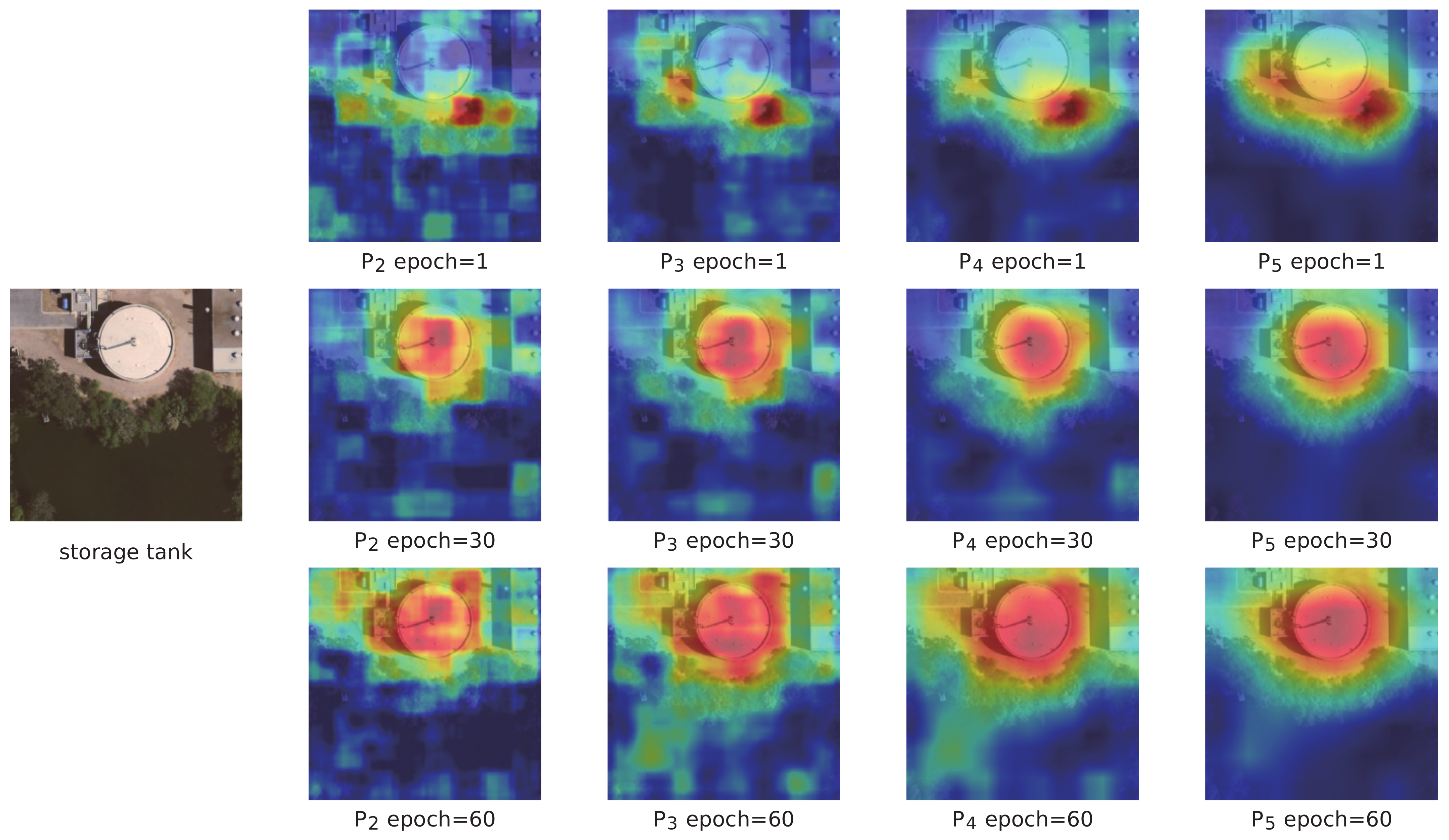
We also selected the UCM dataset to generate the energy maps of ${\mathit{P}}_2$–${\mathit{P}}_5$ at different training stages to explore the branch learning process. As shown in Figure 16 and Figure 17, the attention of the feature map gradually transfers to the discriminative area as the training progresses. Additionally, even the low-level feature map ${\mathit{P}}_2$ can focus on the discriminative area. The results show that our network can extract accurate discriminative regional features and further verify the effectiveness of the self-supervised branch.

Figure 16. An example of an energy map for feature maps ${\mathit{P}}_2$–${\mathit{P}}_5$.

Figure 17. An example of an energy map for feature maps ${\mathit{P}}_2$–${\mathit{P}}_5$.

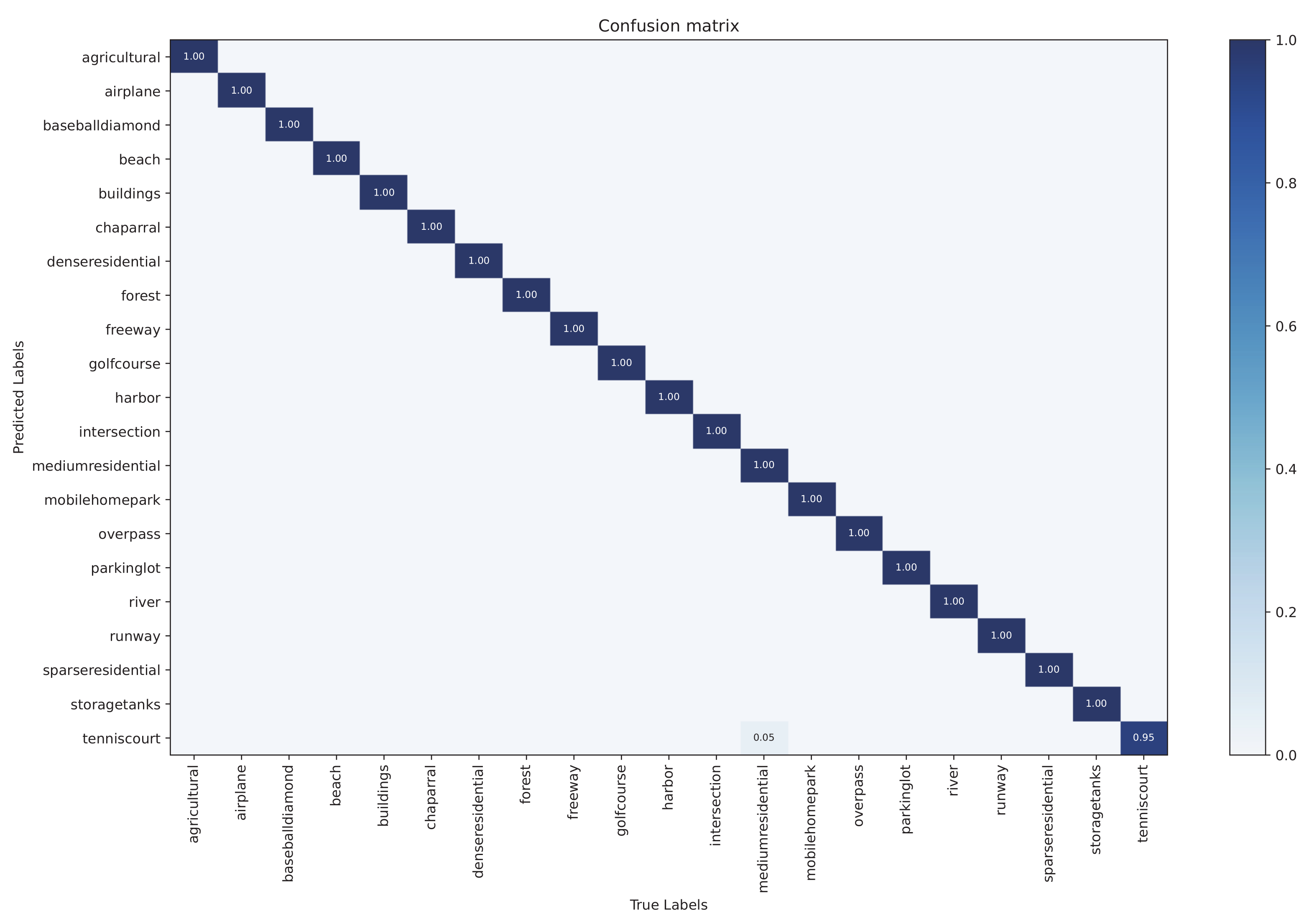
To further demonstrate the classification results of our SSKDNet, we used T-SNE [72] to map the prediction vectors in the high-dimensional space to the low-dimensional space. In addition, we visualize Cycle MLP and SSKDNet by randomly selecting 1000 test samples on the AID and UCM datasets, respectively. Figure 18a,b represent the visualization results of Cycle MLP and SSKDNet on the AID dataset, respectively. Figure 18c,d represent the visualization results of SSKDNet on the UCM dataset, respectively. It can be seen that SSKDNet has smaller intraclass distance and larger interclass distance than Cycle MLP.

Figure 18. Visualization results of predictions of Cycle MLP and SSKDNet on the AID dataset and the UCM dataset. (a,b) represent the T-SNE results on the AID dataset. (c,d) represent the T-SNE results on the UCM dataset.

6. Conclusions

This article investigated the Cycle MLP models for RSISC. We have also proposed the SSKDNet model to improve the discriminative ability of the Cycle MLP model. First, a self-supervised branch is introduced, which generates labels through feature maps to alleviate the problem of insufficient training data. Second, an attention-based feature fusion module is introduced to fuse adjacent feature maps dynamically. Finally, a knowledge distillation method is proposed to distil the “dark knowledge” of the branch to the backbone. Moreover, a multi-task loss function weighting method is introduced to weight the SSKDNet loss function dynamically. We evaluate the performance of our model on three public datasets, achieving 99.62%, 95.96%, and 92.77% accuracy on the UCM, AID, and NWPU datasets, respectively. Results on multiple datasets show that SSKDNet has more competitive classification accuracy than some SOTA methods, and MLP can achieve a similar effect to the self-attention mechanism. For future work, we will try to reduce the time consumption of the SSKDNet method in the training phase and further improve the performance on small-scale datasets.

References

- Cheng, G.; Xie, X.; Han, J.; Guo, L.; Xia, G.S. Remote sensing image scene classification meets deep learning: Challenges, methods, benchmarks, and opportunities. IEEE J. Sel. Top. Appl. Earth Obs. Remote Sens. 2020, 13, 3735–3756. [Google Scholar] [CrossRef]
- Xia, G.S.; Hu, J.; Hu, F.; Shi, B.; Bai, X.; Zhong, Y.; Zhang, L.; Lu, X. AID: A benchmark data set for performance evaluation of aerial scene classification. IEEE Trans. Geosci. Remote Sens. 2017, 55, 3965–3981. [Google Scholar] [CrossRef]
- Xia, G.S.; Bai, X.; Ding, J.; Zhu, Z.; Belongie, S.; Luo, J.; Datcu, M.; Pelillo, M.; Zhang, L. DOTA: A large-scale dataset for object detection in aerial images. In Proceedings of the IEEE Conference on Computer Vision and Pattern Recognition, Salt Lake City, UT, USA, 18–22 June 2018; pp. 3974–3983. [Google Scholar]
- Maggiori, E.; Tarabalka, Y.; Charpiat, G.; Alliez, P. Can semantic labeling methods generalize to any city? the inria aerial image labeling benchmark. In Proceedings of the 2017 IEEE International Geoscience and Remote Sensing Symposium (IGARSS), Fort Worth, TX, USA, 23–28 July 2017; pp. 3226–3229. [Google Scholar]
- Benedek, C.; Szirányi, T. Change detection in optical aerial images by a multilayer conditional mixed Markov model. IEEE Trans. Geosci. Remote Sens. 2009, 47, 3416–3430. [Google Scholar] [CrossRef]
- Liu, J.; Wu, Z.; Xiao, L.; Wu, X.J. Model inspired autoencoder for unsupervised hyperspectral image super-resolution. IEEE Trans. Geosci. Remote Sens. 2022, 60, 1–12. [Google Scholar] [CrossRef]
- Shen, D.; Liu, J.; Wu, Z.; Yang, J.; Xiao, L. ADMM-HFNet: A matrix decomposition-based deep approach for hyperspectral image fusion. IEEE Trans. Geosci. Remote Sens. 2022, 60, 1–17. [Google Scholar] [CrossRef]
- Longbotham, N.; Chaapel, C.; Bleiler, L.; Padwick, C.; Emery, W.J.; Pacifici, F. Very high resolution multiangle urban classification analysis. IEEE Trans. Geosci. Remote Sens. 2011, 50, 1155–1170. [Google Scholar] [CrossRef]
- Martha, T.R.; Kerle, N.; Van Westen, C.J.; Jetten, V.; Kumar, K.V. Segment optimization and data-driven thresholding for knowledge-based landslide detection by object-based image analysis. IEEE Trans. Geosci. Remote Sens. 2011, 49, 4928–4943. [Google Scholar] [CrossRef]
- Cheng, G.; Zhou, P.; Han, J. Learning rotation-invariant convolutional neural networks for object detection in VHR optical remote sensing images. IEEE Trans. Geosci. Remote Sens. 2016, 54, 7405–7415. [Google Scholar] [CrossRef]
- Lv, P.; Wu, W.; Zhong, Y.; Du, F.; Zhang, L. SCViT: A Spatial-Channel Feature Preserving Vision Transformer for Remote Sensing Image Scene Classification. IEEE Trans. Geosci. Remote Sens. 2022, 60, 1–12. [Google Scholar] [CrossRef]
- Dosovitskiy, A.; Beyer, L.; Kolesnikov, A.; Weissenborn, D.; Zhai, X.; Unterthiner, T.; Dehghani, M.; Minderer, M.; Heigold, G.; Gelly, S.; et al. An image is worth 16x16 words: Transformers for image recognition at scale. arXiv 2020, arXiv:2010.11929. [Google Scholar]
- Bazi, Y.; Bashmal, L.; Rahhal, M.M.A.; Dayil, R.A.; Ajlan, N.A. Vision transformers for remote sensing image classification. Remote Sens. 2021, 13, 516. [Google Scholar] [CrossRef]
- Xu, K.; Deng, P.; Huang, H. Vision Transformer: An Excellent Teacher for Guiding Small Networks in Remote Sensing Image Scene Classification. IEEE Trans. Geosci. Remote Sens. 2022, 60, 1–15. [Google Scholar] [CrossRef]
- Liu, H.; Dai, Z.; So, D.; Le, Q.V. Pay attention to mlps. Adv. Neural Inf. Process. Syst. 2021, 34, 9204–9215. [Google Scholar]
- Tolstikhin, I.O.; Houlsby, N.; Kolesnikov, A.; Beyer, L.; Zhai, X.; Unterthiner, T.; Yung, J.; Steiner, A.; Keysers, D.; Uszkoreit, J.; et al. Mlp-mixer: An all-mlp architecture for vision. Adv. Neural Inf. Process. Syst. 2021, 34, 24261–24272. [Google Scholar]
- Tang, C.; Zhao, Y.; Wang, G.; Luo, C.; Xie, W.; Zeng, W. Sparse MLP for Image Recognition: Is Self-Attention Really Necessary? arXiv 2021, arXiv:2109.05422. [Google Scholar] [CrossRef]
- Chen, S.; Xie, E.; Ge, C.; Liang, D.; Luo, P. Cyclemlp: A mlp-like architecture for dense prediction. arXiv 2021, arXiv:2107.10224. [Google Scholar]
- Bi, Q.; Qin, K.; Zhang, H.; Xia, G.S. Local semantic enhanced convnet for aerial scene recognition. IEEE Trans. Image Process. 2021, 30, 6498–6511. [Google Scholar] [CrossRef]
- Yang, Y.; Newsam, S. Bag-of-visual-words and spatial extensions for land-use classification. In Proceedings of the 18th SIGSPATIAL International Conference on Advances in Geographic Information Systems, San Jose, CA, USA, 2–5 November 2010; pp. 270–279. [Google Scholar]
- Noroozi, M.; Favaro, P. Unsupervised learning of visual representations by solving jigsaw puzzles. In Proceedings of the European Conference on Computer Vision, Munich, Germany, 8–14 September 2016; Springer: Berlin/Heidelberg, Germany, 2016; pp. 69–84. [Google Scholar]
- Wang, Q.; Huang, W.; Xiong, Z.; Li, X. Looking closer at the scene: Multiscale representation learning for remote sensing image scene classification. IEEE Trans. Neural Netw. Learn. Syst. 2020, 33, 1414–1428. [Google Scholar] [CrossRef]
- Lin, T.Y.; Dollár, P.; Girshick, R.; He, K.; Hariharan, B.; Belongie, S. Feature pyramid networks for object detection. In Proceedings of the IEEE Conference on Computer Vision and Pattern Recognition, Honolulu, HI, USA, 21–26 July 2017; pp. 2117–2125. [Google Scholar]
- Hu, J.; Shu, Q.; Pan, J.; Tu, J.; Zhu, Y.; Wang, M. MINet: Multilevel Inheritance Network-Based Aerial Scene Classification. IEEE Geosci. Remote Sens. Lett. 2021, 19, 1–5. [Google Scholar] [CrossRef]
- Shen, J.; Yu, T.; Yang, H.; Wang, R.; Wang, Q. An Attention Cascade Global–Local Network for Remote Sensing Scene Classification. Remote Sens. 2022, 14, 2042. [Google Scholar] [CrossRef]
- Liu, S.; Qi, L.; Qin, H.; Shi, J.; Jia, J. Path aggregation network for instance segmentation. In Proceedings of the IEEE Conference on Computer Vision and Pattern Recognition, Salt Lake City, UT, USA, 18–22 June 2018; pp. 8759–8768. [Google Scholar]
- Ji, M.; Shin, S.; Hwang, S.; Park, G.; Moon, I.C. Refine myself by teaching myself: Feature refinement via self-knowledge distillation. In Proceedings of the IEEE/CVF Conference on Computer Vision and Pattern Recognition, Nashville, TN, USA, 20–25 June 2021; pp. 10664–10673. [Google Scholar]
- Ge, Y.; Choi, C.L.; Zhang, X.; Zhao, P.; Zhu, F.; Zhao, R.; Li, H. Self-distillation with Batch Knowledge Ensembling Improves ImageNet Classification. arXiv 2021, arXiv:2104.13298. [Google Scholar]
- Kendall, A.; Gal, Y.; Cipolla, R. Multi-task learning using uncertainty to weigh losses for scene geometry and semantics. In Proceedings of the IEEE Conference on Computer Vision and Pattern Recognition, Salt Lake City, UT, USA, 18–23 June 2018; pp. 7482–7491. [Google Scholar]
- Lowe, D.G. Distinctive image features from scale-invariant keypoints. Int. J. Comput. Vis. 2004, 60, 91–110. [Google Scholar] [CrossRef]
- Swain, M.J.; Ballard, D.H. Color indexing. Int. J. Comput. Vis. 1991, 7, 11–32. [Google Scholar] [CrossRef]
- Haralick, R.M.; Shanmugam, K.; Dinstein, I.H. Textural features for image classification. IEEE Trans. Syst. Man Cybern. 1973, SMC-3, 610–621. [Google Scholar] [CrossRef]
- Dalal, N.; Triggs, B. Histograms of oriented gradients for human detection. In Proceedings of the 2005 IEEE Computer Society Conference on Computer Vision and Pattern Recognition (CVPR’05), San Diego, CA, USA, 20–26 June 2005; Volume 1, pp. 886–893. [Google Scholar]
- Jégou, H.; Perronnin, F.; Douze, M.; Sánchez, J.; Pérez, P.; Schmid, C. Aggregating local image descriptors into compact codes. IEEE Trans. Pattern Anal. Mach. Intell. 2011, 34, 1704–1716. [Google Scholar] [CrossRef]
- Li, Q.; Yan, D.; Wu, W. Remote Sensing Image Scene Classification Based on Global Self-Attention Module. Remote Sens. 2021, 13, 4542. [Google Scholar] [CrossRef]
- Wu, X.; Zhang, Z.; Zhang, W.; Yi, Y.; Zhang, C.; Xu, Q. A convolutional neural network based on grouping structure for scene classification. Remote Sens. 2021, 13, 2457. [Google Scholar] [CrossRef]
- Shi, C.; Zhao, X.; Wang, L. A multi-branch feature fusion strategy based on an attention mechanism for remote sensing image scene classification. Remote Sens. 2021, 13, 1950. [Google Scholar] [CrossRef]
- Shi, C.; Zhang, X.; Sun, J.; Wang, L. Remote Sensing Scene Image Classification Based on Self-Compensating Convolution Neural Network. Remote Sens. 2022, 14, 545. [Google Scholar] [CrossRef]
- Shi, C.; Zhang, X.; Sun, J.; Wang, L. Remote Sensing Scene Image Classification Based on Dense Fusion of Multi-level Features. Remote Sens. 2021, 13, 4379. [Google Scholar] [CrossRef]
- Ma, A.; Yu, N.; Zheng, Z.; Zhong, Y.; Zhang, L. A Supervised Progressive Growing Generative Adversarial Network for Remote Sensing Image Scene Classification. IEEE Trans. Geosci. Remote Sens. 2022, 60, 1–18. [Google Scholar] [CrossRef]
- Gu, S.; Zhang, R.; Luo, H.; Li, M.; Feng, H.; Tang, X. Improved SinGAN integrated with an attentional mechanism for remote sensing image classification. Remote Sens. 2021, 13, 1713. [Google Scholar] [CrossRef]
- Ma, C.; Sha, D.; Mu, X. Unsupervised adversarial domain adaptation with error-correcting boundaries and feature adaption metric for remote-sensing scene classification. Remote Sens. 2021, 13, 1270. [Google Scholar] [CrossRef]
- Xu, K.; Huang, H.; Deng, P.; Li, Y. Deep feature aggregation framework driven by graph convolutional network for scene classification in remote sensing. IEEE Trans. Neural Netw. Learn. Syst. 2021. [Google Scholar] [CrossRef]
- Peng, F.; Lu, W.; Tan, W.; Qi, K.; Zhang, X.; Zhu, Q. Multi-Output Network Combining GNN and CNN for Remote Sensing Scene Classification. Remote Sens. 2022, 14, 1478. [Google Scholar] [CrossRef]
- Zhang, W.; Tang, P.; Zhao, L. Remote sensing image scene classification using CNN-CapsNet. Remote Sens. 2019, 11, 494. [Google Scholar] [CrossRef]
- Peng, C.; Li, Y.; Jiao, L.; Shang, R. Efficient convolutional neural architecture search for remote sensing image scene classification. IEEE Trans. Geosci. Remote Sens. 2020, 59, 6092–6105. [Google Scholar] [CrossRef]
- Li, L.; Yao, X.; Cheng, G.; Han, J. AIFS-DATASET for Few-Shot Aerial Image Scene Classification. IEEE Trans. Geosci. Remote Sens. 2022, 60, 1–11. [Google Scholar] [CrossRef]
- He, K.; Zhang, X.; Ren, S.; Sun, J. Deep residual learning for image recognition. In Proceedings of the IEEE Conference on Computer Vision and Pattern Recognition, Las Vegas, NV, USA, 27–30 June 2016; pp. 770–778. [Google Scholar]
- Hao, S.; Wu, B.; Zhao, K.; Ye, Y.; Wang, W. Two-Stream Swin Transformer with Differentiable Sobel Operator for Remote Sensing Image Classification. Remote Sens. 2022, 14, 1507. [Google Scholar] [CrossRef]
- Liu, Z.; Lin, Y.; Cao, Y.; Hu, H.; Wei, Y.; Zhang, Z.; Lin, S.; Guo, B. Swin transformer: Hierarchical vision transformer using shifted windows. In Proceedings of the IEEE/CVF International Conference on Computer Vision, Montreal, BC, Canada, 11–17 October 2021; pp. 10012–10022. [Google Scholar]
- Dong, X.; Bao, J.; Chen, D.; Zhang, W.; Yu, N.; Yuan, L.; Chen, D.; Guo, B. Cswin transformer: A general vision transformer backbone with cross-shaped windows. arXiv 2021, arXiv:2107.00652. [Google Scholar]
- Doersch, C.; Gupta, A.; Efros, A.A. Unsupervised visual representation learning by context prediction. In Proceedings of the IEEE International Conference on Computer Vision, Santiago, Chile, 7–13 December 2015; pp. 1422–1430. [Google Scholar]
- Wang, X.; Gupta, A. Unsupervised Learning of Visual Representations Using Videos. In Proceedings of the IEEE International Conference on Computer Vision, Santiago, Chile, 7–13 December 2015; pp. 2794–2802. [Google Scholar]
- Devlin, J.; Chang, M.W.; Lee, K.; Toutanova, K. Bert: Pre-training of deep bidirectional transformers for language understanding. arXiv 2018, arXiv:1810.04805. [Google Scholar]
- He, K.; Chen, X.; Xie, S.; Li, Y.; Dollár, P.; Girshick, R. Masked autoencoders are scalable vision learners. arXiv 2021, arXiv:2111.06377. [Google Scholar]
- Zhao, Z.; Luo, Z.; Li, J.; Chen, C.; Piao, Y. When self-supervised learning meets scene classification: Remote sensing scene classification based on a multitask learning framework. Remote Sens. 2020, 12, 3276. [Google Scholar] [CrossRef]
- Stojnic, V.; Risojevic, V. Self-supervised learning of remote sensing scene representations using contrastive multiview coding. In Proceedings of the IEEE/CVF Conference on Computer Vision and Pattern Recognition, Nashville, TN, USA, 20–25 June 2021; pp. 1182–1191. [Google Scholar]
- Hinton, G.; Vinyals, O.; Dean, J. Distilling the knowledge in a neural network. arXiv 2015, arXiv:1503.02531. [Google Scholar]
- Tung, F.; Mori, G. Similarity-preserving knowledge distillation. In Proceedings of the IEEE/CVF International Conference on Computer Vision, Seoul, Korea, 2 November 2019; pp. 1365–1374. [Google Scholar]
- Zagoruyko, S.; Komodakis, N. Paying more attention to attention: Improving the performance of convolutional neural networks via attention transfer. arXiv 2016, arXiv:1612.03928. [Google Scholar]
- Pande, S.; Banerjee, A.; Kumar, S.; Banerjee, B.; Chaudhuri, S. An adversarial approach to discriminative modality distillation for remote sensing image classification. In Proceedings of the IEEE/CVF International Conference on Computer Vision Workshops, Seoul, Korea, 27–28 October 2019. [Google Scholar]
- Zhao, H.; Sun, X.; Gao, F.; Dong, J. Pair-Wise Similarity Knowledge Distillation for RSI Scene Classification. Remote Sens. 2022, 14, 2483. [Google Scholar] [CrossRef]
- Chen, G.; Zhang, X.; Tan, X.; Cheng, Y.; Dai, F.; Zhu, K.; Gong, Y.; Wang, Q. Training small networks for scene classification of remote sensing images via knowledge distillation. Remote Sens. 2018, 10, 719. [Google Scholar] [CrossRef]
- Zhang, R.; Chen, Z.; Zhang, S.; Song, F.; Zhang, G.; Zhou, Q.; Lei, T. Remote sensing image scene classification with noisy label distillation. Remote Sens. 2020, 12, 2376. [Google Scholar] [CrossRef]
- Cheng, G.; Han, J.; Lu, X. Remote sensing image scene classification: Benchmark and state of the art. Proc. IEEE 2017, 105, 1865–1883. [Google Scholar] [CrossRef]
- Loshchilov, I.; Hutter, F. Decoupled weight decay regularization. arXiv 2017, arXiv:1711.05101. [Google Scholar]
- He, N.; Fang, L.; Li, S.; Plaza, J.; Plaza, A. Skip-connected covariance network for remote sensing scene classification. IEEE Trans. Neural Netw. Learn. Syst. 2019, 31, 1461–1474. [Google Scholar] [CrossRef] [PubMed]
- Zhao, Z.; Li, J.; Luo, Z.; Li, J.; Chen, C. Remote sensing image scene classification based on an enhanced attention module. IEEE Geosci. Remote Sens. Lett. 2020, 18, 1926–1930. [Google Scholar] [CrossRef]
- Shi, C.; Wang, T.; Wang, L. Branch feature fusion convolution network for remote sensing scene classification. IEEE J. Sel. Top. Appl. Earth Obs. Remote Sens. 2020, 13, 5194–5210. [Google Scholar] [CrossRef]
- Yu, D.; Xu, Q.; Guo, H.; Zhao, C.; Lin, Y.; Li, D. An efficient and lightweight convolutional neural network for remote sensing image scene classification. Sensors 2020, 20, 1999. [Google Scholar] [CrossRef]
- Bai, L.; Liu, Q.; Li, C.; Ye, Z.; Hui, M.; Jia, X. Remote Sensing Image Scene Classification Using Multiscale Feature Fusion Covariance Network with Octave Convolution. IEEE Trans. Geosci. Remote Sens. 2022, 60, 1–14. [Google Scholar] [CrossRef]
- Van der Maaten, L.; Hinton, G. Visualizing data using t-SNE. J. Mach. Learn. Res. 2008, 9, 2579–2605. [Google Scholar]
Publisher’s Note: MDPI stays neutral with regard to jurisdictional claims in published maps and institutional affiliations. |
© 2022 by the authors. Licensee MDPI, Basel, Switzerland. This article is an open access article distributed under the terms and conditions of the Creative Commons Attribution (CC BY) license (https://creativecommons.org/licenses/by/4.0/).