Spatio-Temporal Dynamics and Driving Forces of Multi-Scale CO₂ Emissions by Integrating DMSP-OLS and NPP-VIIRS Data: A Case Study in Beijing-Tianjin-Hebei, China

Abstract

The emission of greenhouse gases, especially CO₂, is the main factor causing global warming. Due to incomplete statistical data on energy consumption at and below the urban scale of Beijing-Tianjin-Hebei (BTH), in this study, Defense Meteorological Satellite Program Operational Linescan System (DMSP-OLS) and Suomi National Polar-orbiting Partnership Visible Infrared Imaging Radiometer Suite (NPP-VIIRS) data were combined, and a neural network model and weighted average method based on DN (Digital Number) value were used to obtain CO₂ emissions at the municipal and county scales with a resolution of 1 km × 1 km from 2000–2019. Next, a spatial-temporal analysis model and spatial econometric model were used to study the CO₂ emissions at different scales of BTH. This study also solved the problem that STIRPAT analysis cannot be carried out due to insufficient urban statistical CO₂ emissions data. The results show that the energy CO₂ emissions in BTH present a distribution pattern of “East greater than West”, with a trend of first rising and then slowing down. Moreover, the rapid growth areas are mainly located in Chengde and Tianjin. The degree of regional spatial aggregation decreased year by year from 2000–2019. Population, affluence and technology factors were positively correlated with CO₂ emissions in Tianjin and Hebei. For Beijing, in addition to foreign investment, factors such as urbanization rate, energy intensity, construction and transportation factors all contributed to the increase in CO₂ emissions. Among them, the growth of population is the main reason for the increase of CO₂ at the urban scale in BTH. Finally, based on the research results and the specific situation of the cities, corresponding policies and measures are proposed for the future low-carbon development of the cities.

1. Introduction

In recent years, global warming has become an indisputable fact. Greenhouse gas emissions, especially CO₂ emissions, have been proven to be one of the main causes of global warming [1]. However, for densely populated urban areas, CO₂ from the burning of fossil fuels from human activities is the main source of global CO₂ emissions [2]. Urban regions utilized 75% of the world’s energy and emitted 80% of global greenhouse gas emissions, even though they cover less than 3% of the Earth’s surface [3]. Over the past century, CO₂ emissions have significantly increased due to the ongoing rise in energy consumption brought on by the process of global economic development [4]. China, a significant developing nation, since 2006, has ranked first in the world for CO₂ emissions [5]. China’s CO₂ emissions have increased significantly due to the country’s increasing industrialization and urbanization. According to the energy statistics provided by the International Energy Agency (IEA), China accounted for 28.13% of global CO₂ emissions in 2015, exceeding the combined emissions of the United States and the European Union [6]. China is facing serious environmental problems and pressure to deal with climate change. Thus, understanding the spatial and temporal distribution of CO₂ emissions at different administrative levels is crucial for China’s future development [7].

In September 2020, China proposed the “dual carbon” goal. That is, China will work to peak its CO₂ emissions before 2030 and to become carbon neutral before 2060 [8]. In order to achieve this goal, China has clearly put forward the main implementation paths and policy proposals in many aspects. Due to the vast territory and uneven economic development level, the BTH region, as the key area of the Bohai economic circle, is the most energy-intensive region in China. Despite accounting for only 2.3% of China’s total land area, the BTH contributed almost 15% of China’s CO₂ emissions in 2018 [9]. As a result, the region must transition to low-carbon development to meet China’s carbon reduction targets. However, there are huge differences amongst cities in terms of economic and social growth. Therefore, the analysis of CO₂ distribution and driving forces in different scale regions can contribute significantly to the formulation of urban development strategies and the future planning of BTH.

A detailed spatio-temporal analysis of carbon emissions can provide a basis for CO₂ emission strategies in different regions. Many previous studies have assessed energy consumption in different countries and regions at different scales [10,11,12]. However, most of the studies on CO₂ emissions in the BTH region concentrated on the municipalities (Beijing, Tianjin) and provinces (Hebei), and most of them were based on statistics from the national and provincial energy administrations, which only provided a digital record of CO₂ emissions by administrative units, but did not reveal their spatial distribution characteristics. According to numerous earlier studies, nighttime lighting data is a valuable indicator for assessing human activities and social economy, such as estimating regional populations [13,14], urban expansion [15], economic development [16], power consumption [17], gas combustion [18], etc. Based on DMSP-OLS data, many scholars have conducted regression analyses on the nighttime stable light (NSL) and CO₂ emission index, and confirmed that nighttime lighting data at the national, provincial and municipal levels and CO₂ emissions are significantly correlated [19,20]. Therefore, using nighttime light data opens a new perspective for dynamic monitoring of energy consumption. The studies of Zhang [20] and Zhao [21] showed that two types of nighttime light data both have benefits at different scales, and their combination can be used to investigate the spatial patterns of CO₂ emissions in long time series. Lv [22] integrated and analyzed the spatio-temporal dynamics of CO₂ emissions in China by using two nighttime lighting datasets, and her research results proved that DMSP-OLS and NPP-VIIRS data could be effectively combined to study CO₂ emissions. Meng [23] used linear equations to fit night light data and CO₂ data based on DMSP-OLS data. Considering that there is a nonlinear relationship between CO₂ emission and light value, conventional econometric methods may produce large errors [24]. The majority of the studies mentioned above were conducted on large-scale regions, such as national and provincial levels, lacking detailed studies on city and county scales, and are based on a single satellite. It is more necessary to meet the high accuracy of fitting the CO₂ emission and nighttime light values for the investigation of small-scale areas.

Previously conducted research on the influencing factors of CO₂ emissions primarily included logarithmic average weight, the Divisia decomposition method, the LMDI decomposition method, IPAT theory and the STIRPAT model, the factor decomposition method, Kuznets curve theory and the spatial econometric model and other methods and theories [25,26,27,28]. The IPAT model is widely used as a classical model to study CO₂ emissions [29,30]. Since this model cannot make assumptions on variables, York [31] proposed an improved model, the STIRPAT model, based on the IPAT model, which removed the influence of the same proportion change. The model comprehensively considers the impact of population, affluence and technology on the environment, and is widely used in various fields. But they are mostly used at the national and provincial levels, and few studies have been conducted at the city level, where data on CO₂ emissions are lacking. Therefore, in order to overcome the drawback that STIRPAT cannot be utilized to examine urban carbon emissions due to a lack of data, this study combines the two kinds of nighttime lighting data (DMSP-OLS and NPP-VIIRS) to get municipal carbon emission data.

The remainder of this paper is organized as follows. Section 2 describes the study area and data sources. Section 3 outlines the integration of DMSP-OLS with NPP-VIIRS data, as well as the estimation of CO₂ emissions at the city and county scales and the assessment of the characteristics of spatial and temporal changes in carbon emissions and the analysis of driving forces. Section 4 analyzes the main results obtained in this paper. Section 5 discusses the results. Finally, Section 6 lists the main conclusions and puts forward some strategies for the future low-carbon development of BTH.

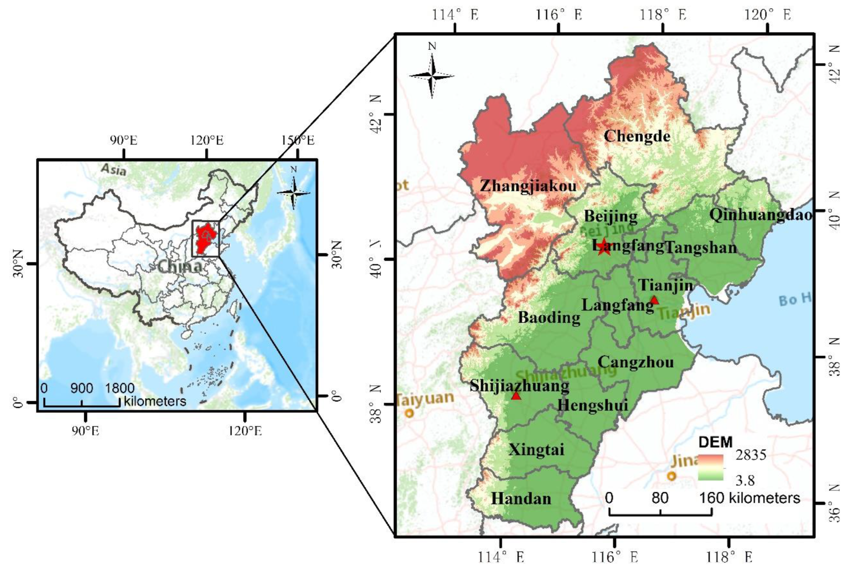
2. Study Areas and Data Sources

The study area includes Beijing, Tianjin and the Hebei Province, which are located in the North China Plain, accounting for 2.27% of the total land area of China. The area is the center of Chinese politics, culture, economy, science and technology, and it is also the area where Chinese steel production is most concentrated. The analysis process involved 13 cities, 199 counties and other administrative units (Figure 1).

DMSP-OLS nighttime lighting data was obtained from the National Oceanic and Atmospheric Administration’s National Geophysical Data Center (NOAA/NGDC) website (https://ngdc.noaa.gov/eog/dmsp/downloadV4composites.html (accessed on 1 March 2022)). The product spans from 1992–2013, and the image is generated by six separate sensors, these being F10 (1992–1994), F12 (1994–1999), F14 (1997–2003), F15 (2000–2007), F16 (2004–2009), and F18 (2010–2013). Four sensor data, F14, F15, F16 and F18, were used in this study. The illumination area is large, but there is an obvious saturation problem, and the DN value ranges from 0–63. Annual data from version four of DMSP-OLS from 2000–2013 was used in this study. NPP-VIIRS, which was launched in 2011, is an Earth observation satellite NPP equipped with a visible/infrared radiation imager (VIIRS) which obtains remote sensing images of ground light at night in the DNB (Day/Night Band) band. This study selected monthly data from 2012–2019, obtained from the website (https://eogdata.mines.edu/products/vnl/ (accessed on 5 March 2022)).

All statistical data were obtained from the China Energy Statistical Yearbook, the China Urban Statistical Yearbook and local statistical yearbooks, the Beijing Statistical Yearbook, the Tianjin Statistical Yearbook, and the Hebei Statistical Yearbook.

3. Methodology

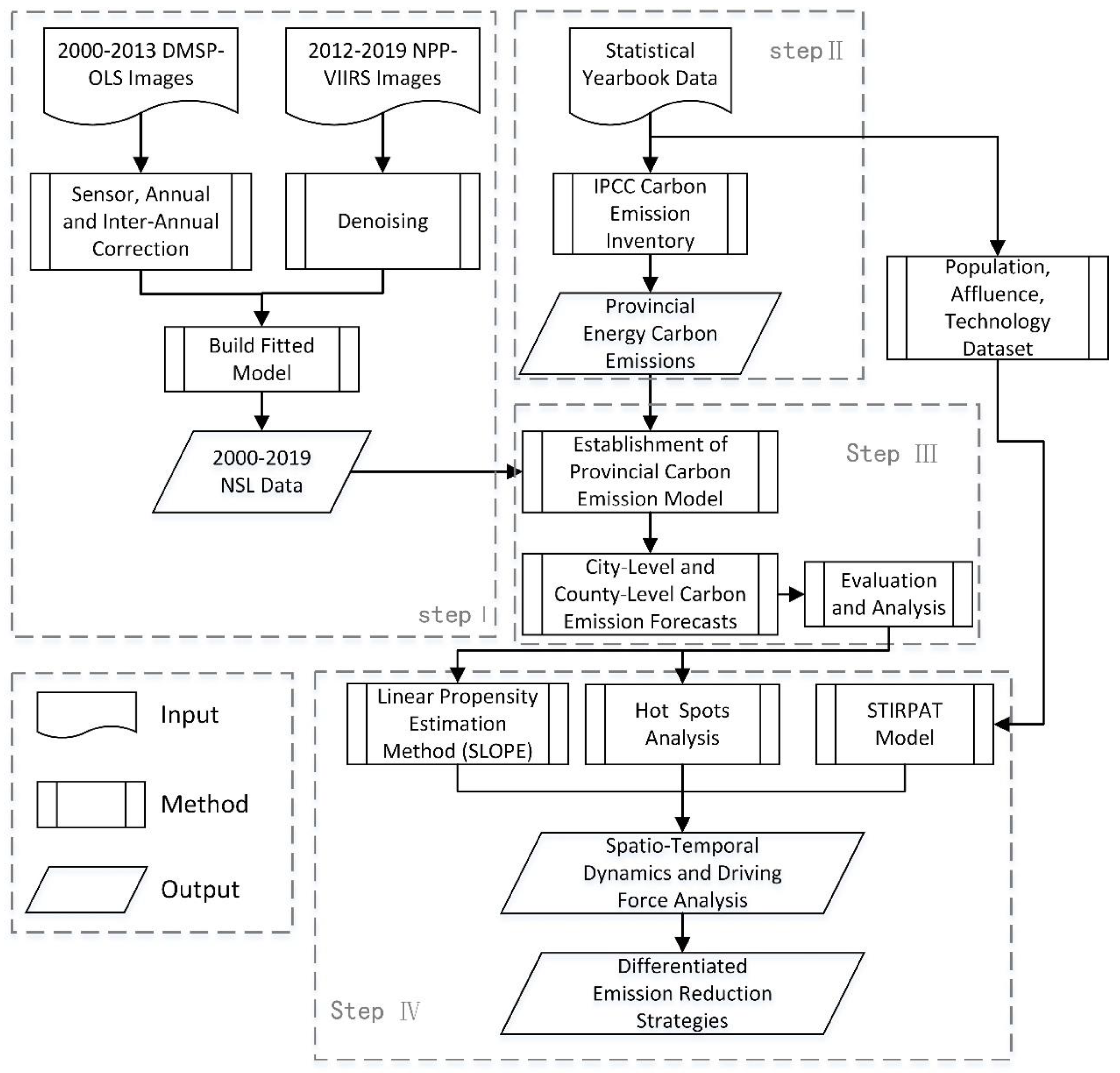
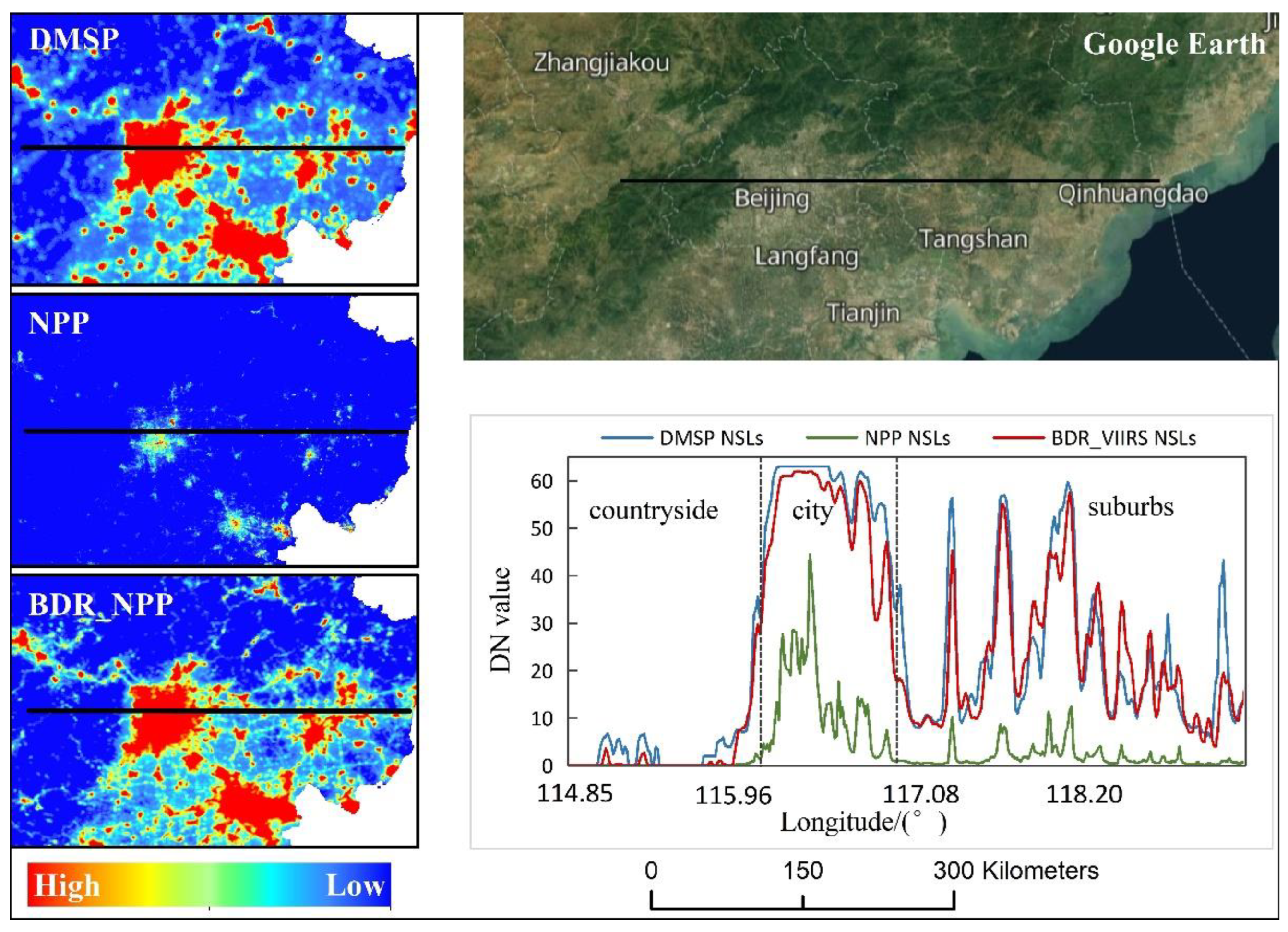
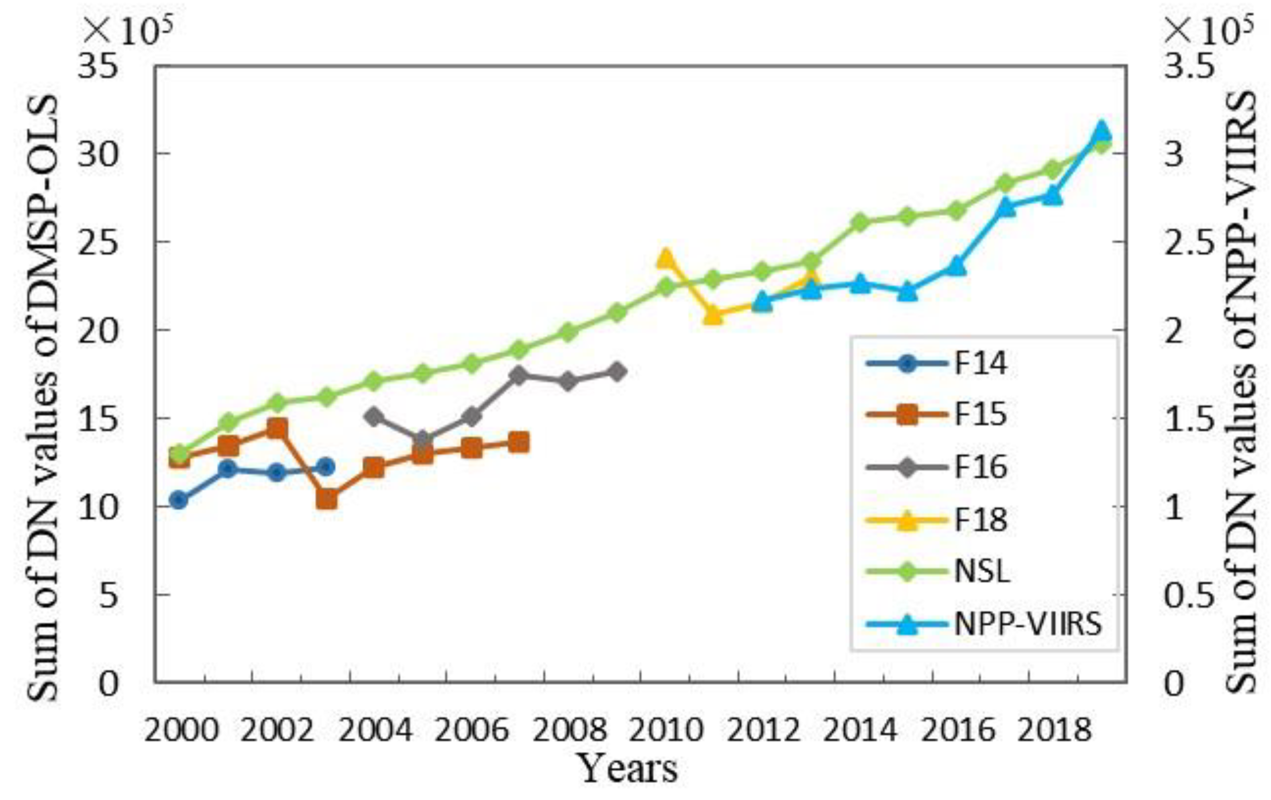
3.1. Integration of Two Kinds of Night Light Data

The integration of the two kinds of night light data is mainly divided into three steps (Figure 2):

• DMSP-OLS data were corrected by sensor, within year and between years;
• Annual synthesis and denoising of NPP-VIIRS data;
• Using a model to integrate the former two datasets to obtain the stable nighttime lighting data from 2000–2019.

Because NPP-VIIRS are the monthly average data and are polluted by stray light, the light data from May to July in the middle and high latitude areas of summer in China are seriously distorted, and the pixel value is 0. Therefore, the missing months were eliminated and the other months were synthesized to obtain the annual comprehensive data. The images and DMSP-OLS images were then resampled to 1 km × 1 km and projected onto the Albers equal area projection. The invariant region method was selected to carry out sensor correction, annual correction and inter-annual correction for DMSP-OLS data, and then the continuity was improved. For the specific method, we referred to the study of Elvidge [18]. After viewing the distribution of the data, it was found that approximately 99% of the pixel values were low (DN < 0.3). In order to remove the weak light in the NPP-VIIRS data (usually regarded as noise), the threshold method was used to correct it, and 0.3 × 10⁻⁹ W·cm⁻²·sr⁻¹ was used as the empirical threshold, while values less than 0.3 in the NPP-VIIRS data was assigned as 0 [32]. Because there were abnormally high light values in NPP-VIIRS images, the method of Zhao [33] was adopted in this paper. The pixel values higher than those of China’s three megacities (Beijing, Shanghai and Guangzhou) (DN_MAX) in other regions were considered as outliers caused by oil, gas or fire. Each outlier was iterated to the maximum value in its respective 3 × 3 neighborhood raster DN until no value exceeded DN_MAX.

Because of the dispersion of the two groups of data, it is difficult to fit the data directly, so the coefficient of variation (cv) method was used to deal with this problem [34]. The NPP-VIIRS data in 2012 was only available for six months, so the cv values of all pixel 3 × 3 windows in NPP-VIIRS and DMSP-OLS data of 2013 were chosen to be calculated. The cv value is calculated using the following formula:

$$cv=\frac{S}{x}$$

(1)

where $S$ and $x$ are the standard deviation and average value of the image radiation value, respectively.

Subsequently, the NPP-VIIRS data were log-transformed to reduce the difference between the two datasets and make the brightness range consistent with the DMSP-OLS data.

$$Log\_V_i=Ln\left(V_i+1\right)$$

(2)

where $V_i$ is the original radiation value of NPP-VIIRS, and $Log\_V_i$ is the result after logarithmic transformation. In order to make the logarithmic transformation valid, we added the constant 1 to the equation.

According to previous studies, the two groups of cv values show an S-shape after fitting (Figure 3), and ordinary function curves are difficult to fit accurately. In this study, the S-type function model BiDoseResp was adopted to integrate the two kinds of night lights. Meanwhile, in order to ensure its accurate application in the Beijing-Tianjin-Hebei region, unary linear regression, binary linear regression and the DoseResp function model were used for comparison. Finally, the results showed that the BiDoseResp model worked best among the four models. The order of R² was BiDoseResp (0.8836) > DoseResp (0.8833) > binomial (0.8378) > unary linear (0.8359), and the RSS of the BiDoseResp model was the smallest, which was 3.4687 × 10⁵. Its model parameters are shown in

Table 1. BiDoseResp model coefficients.

A1	A2	LOGx01	LOGx02	h1	h2	P
−35.4269	64.19793	0.36666	−1.98149	2.24954	0.41862	0.47464

. The BiDoseResp formula can be expressed as follows:

$$y=A1+\left(A2-A1\right)\left[\frac{p}{1+{10}^{\left(LOGx01-x\right)h1}}+\frac{1-p}{1+{10}^{\left(LOGx02-x\right)h2}}\right]$$

(3)

where $A1$ and $A2$ are the minimum and maximum of the function, respectively, $p$ represents the weight of Logistic, $LOGx01$ and $LOGx02$ respectively represent the average value of the independent variables of the two curves, and $h1$ and $h2$ represent the curve slope 1 and slope 2, respectively. Finally, the obtained NPP-VIIRS data was processed by Gaussian low-pass filtering to obtain a smooth image.

3.2. Estimating CO₂ Emissions According to IPCC

The United Nations’ Intergovernmental Panel on Climate Change (IPCC) provided the internationally agreed standard for assessing emissions of the greenhouse gas CO₂. This study used the IPCC method to calculate the CO₂ emissions of each province and city from 2000–2019. The formula is as follows:

$$Y_{C{O}_2}=\frac{44}{12}\times {\displaystyle \sum _{i=1}^n{K}_i}{E}_i$$

(4)

where $i$ is the type of energy, $n$ represents the quantity of energy, $E_i$ represents the consumption of energy type $i$ (calculated by standard coal), and $K_i$ represents the carbon emission coefficient of energy $i$, the original data unit is J, and in order to keep the data unit consistent, it is converted into standard coal (SCE); the conversion coefficient is: 1 × 10⁴ t standard coal is equal to 2.93 × 10⁵ GJ. 44/12 is the amount of carbon dioxide produced by the complete combustion of one ton of carbon in oxygen.

Table 2. Fossil energy emission factors.

Energy Type	SCE Conversion Factor (tSCE/t)	CO2 Emission Factor (t/SCE)
Raw coal	0.7143	0.7559
Coke	0.9714	0.855
Crude oil	1.4286	0.5857
Gasoline	1.4714	0.5538
Kerosene	1.4714	0.5714
Diesel fuel	1.4571	0.5921
Fuel oil	1.4286	0.6185
Natural gas	13.3	0.4483
Electricity	1.229	0.272

Note: The conversion of natural gas into standard coal is standard coal/10,000 m³, and the conversion of electricity into standard coal is standard coal/10,000 kWh.

lists the conversion of carbon emission coefficient and standard coal of different fossil fuels. These energy sources account for about 85% of China’s total emissions.

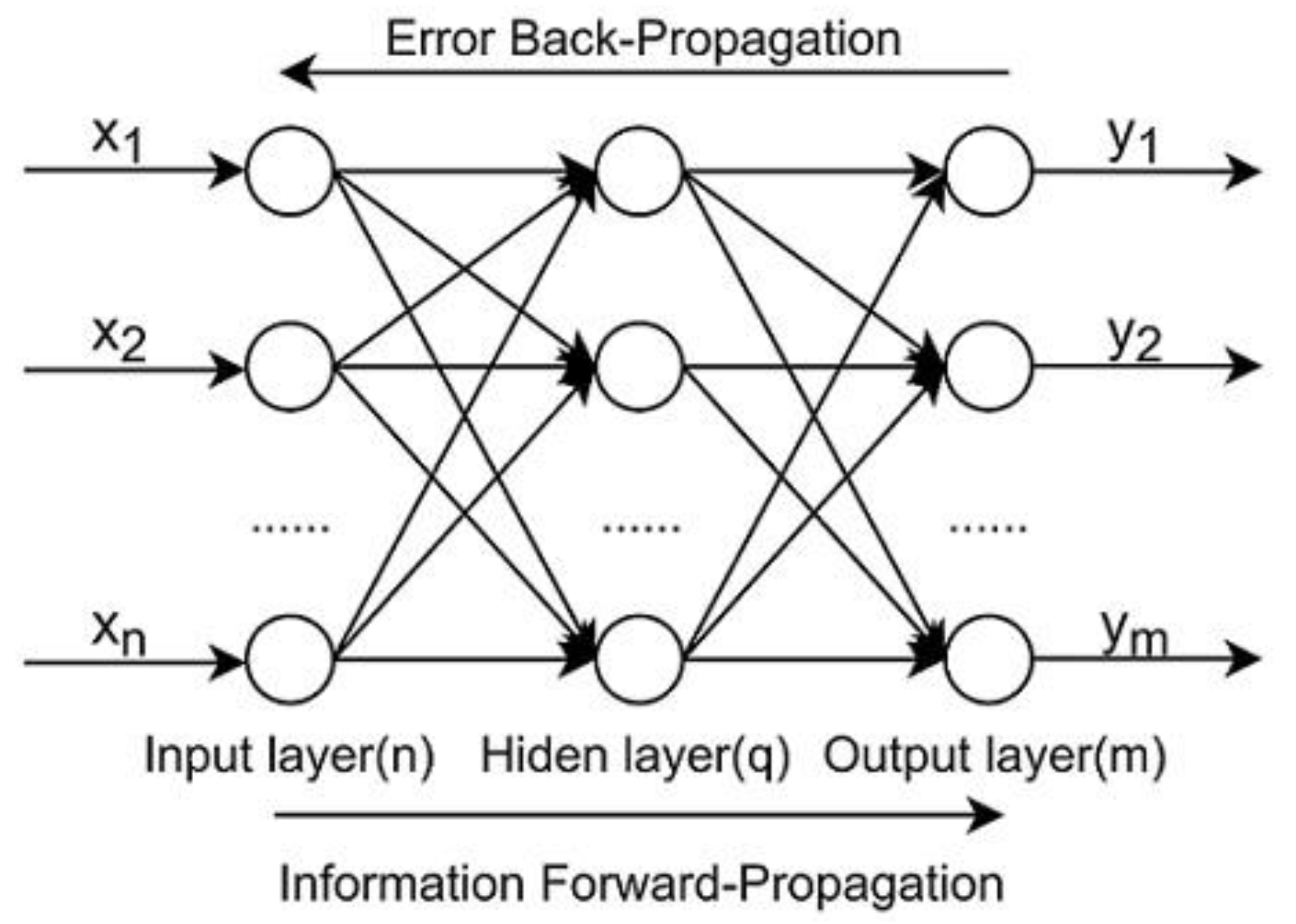
3.3. Estimating CO₂ Emissions at Municipal and County Levels

Regression modeling can be used to determine the association between CO₂ emissions and NSL. Due to the nonlinear relationship between CO₂ emissions and NSL, the traditional methods may lead to relatively high errors, especially for Beijing. Artificial neural networks can effectively solve this problem. It is a kind of machine learning, which is a nonlinear, dynamic and complex information processing system connected by a large number of neurons. Bp-neural networks are a kind of multi-layer feedforward neural network which is trained according to the error back propagation method (Figure 4), which generally includes three layers: the input layer, the hidden layer and the output layer, and each layer has multiple nodes. Therefore, we chose the BP-neural network method to fit NSL and CO₂ emission data. $x={\left[x_1,x_2,\dots ,x_n\right]}^{\mathrm{T}}$ was selected as the DN value of NSL, $y={\left[y_1,y_2,\dots ,y_m\right]}^{\mathrm{T}}$ was selected as the CO₂ emission data as the output value, and $W_{ij}$ was the weight parameter. Considering the accuracy of the BP-neural network, 70% of the samples were used as the training set, and 30% of the samples were used as the test set and validation set. Since the types of economic development in Hebei Province, Beijing and Tianjin are quite different, Hebei Province was chosen to be fitted separately.

The relationship between input and output during forward propagation is as follows:

$$y_j={\displaystyle \sum _{i=1}^m{\omega }_{ij}}{x}_i+b_j$$

(5)

$$x_j=f\left(y_j\right)=\frac{1}{1+e^{-y_j}}$$

(6)

The gradient descent method is adopted for reverse error propagation, and the loss function is:

$$E=\frac{1}{2}{\displaystyle \sum _{j=1}^p{\left(x_j-y_j\right)}^2}$$

(7)

The revised weight value and threshold calculation formula are:

$$W_{ij}=w_{ij}+\mathrm{\Delta }{w}_{ij}$$

(8)

$$B_j=b_j+\mathrm{\Delta }{b}_j$$

(9)

$$\mathrm{\Delta }{w}_{ij}=-{\eta }_1\frac{\partial E}{\partial w_{ij}}$$

(10)

$$\mathrm{\Delta }{b}_j=-{\eta }_2\frac{\partial E}{\partial b_j}$$

(11)

where $x_i$ is the input value of node $i$, $x_j$ is the output value of node $j$, $y_j$ is the net output value of node $j$, ${\omega }_{ij}$ represents the weight between nodes $i$ and $j$, and $b_j$ represents the threshold of node $j$, $f$ is the transfer function of the node, $p$ is the number of iterations; $W_{ij}$ and $B_j$ are the weight correction amount and the threshold between the $i$ node and the $j$ node, respectively.

In order to obtain CO₂ emission data at the city, district and county level, the weighted average method based on $DN$ value was used in this study. The formula is as follows:

$$C_i=D{N}_i\times \frac{y_m}{{\displaystyle {\sum }_{i=1}^{n}D{N}_i}}$$

(12)

where $i$ stands for different cities ($i$= 1,2,3...$n$), $m$ represents the province where city $i$ is located, $C_i$ represents the CO₂ emissions of city $i$, $y_m$ represents the CO₂ emissions of province $m$.

3.4. Analysis of Spatio-Temporal Pattern

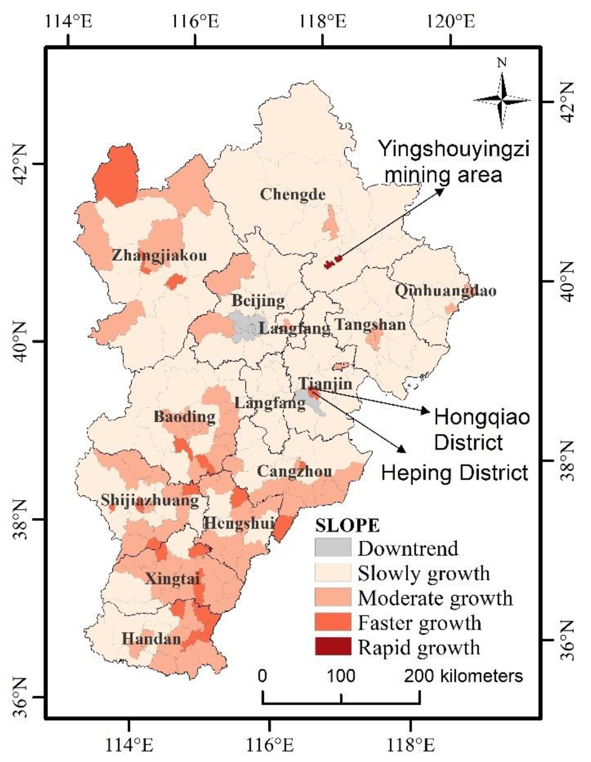
3.4.1. Linear Propensity Estimation (Slope)

The linear propensity estimation method was used to obtain the propensity values of each county in different years from 2000–2019 so as to analyze the changing trends and types of carbon emissions. With the change of time, energy emissions will show a significant increase, a significant decline, or no obvious change. The area with a tendency value less than 0 is classified as having a downward trend, while the area with a tendency value greater than 0 is classified as having one of four growth speeds: slow, medium, faster, and rapid. It is calculated as follows:

$$SLOPE=\frac{n\times {\displaystyle {\sum }_{i=1}^n{x}_i{C}_i-{\displaystyle {\sum }_{i=1}^n{x}_i{\displaystyle {\sum }_{i=1}^n{C}_i}}}}{n\times {\displaystyle {\sum }_{i=1}^n{C}_i{}^2-{\left({\displaystyle {\sum }_{i=1}^n{C}_i}\right)}^2}}$$

(13)

where $n$ is the total number of years, which is 20; $C_i$ is the CO₂ emissions in the year $i$, $x_i$ is the year $i$.

3.4.2. Global Autocorrelation

The global Moran’s I index can judge the spatial distribution pattern of carbon emissions in Beijing-Tianjin-Hebei by reflecting the similarity or correlation degree of carbon emissions in the spatially adjacent regions. The specific formula is as follows:

$$I=\frac{n{\displaystyle \sum _{i=1}^n{\displaystyle \sum _{j=1}^n{w}_{ij}\left(x_i-\overline{x}\right)\left(x_j-\overline{x}\right)}}}{{\displaystyle \sum _{i=1}^n{\displaystyle \sum _{j=1}^n{w}_{ij}{\displaystyle \sum _{i=1}^n{\left(x_i-\overline{x}\right)}^2}}}}$$

(14)

where $I$ is the global Moran’s I index, $x_i$ and $x_j$ represent the CO₂ emission values of county $i$ and county $j$, $n$ is the total number of units in the districts and counties, and $w_{ij}$ is the standardized spatial weight matrix.

When the Moran index is greater than 0, it indicates that there is a positive correlation between regions; otherwise, there is a negative correlation. The Z-value size can judge the significance level; if |Z| ≤ 1.96 and p ≥ 0.05, it means that there is no correlation in the region; if |Z| ≥ 1.96, p < 0.05, it means that there is significant spatial autocorrelation in the region.

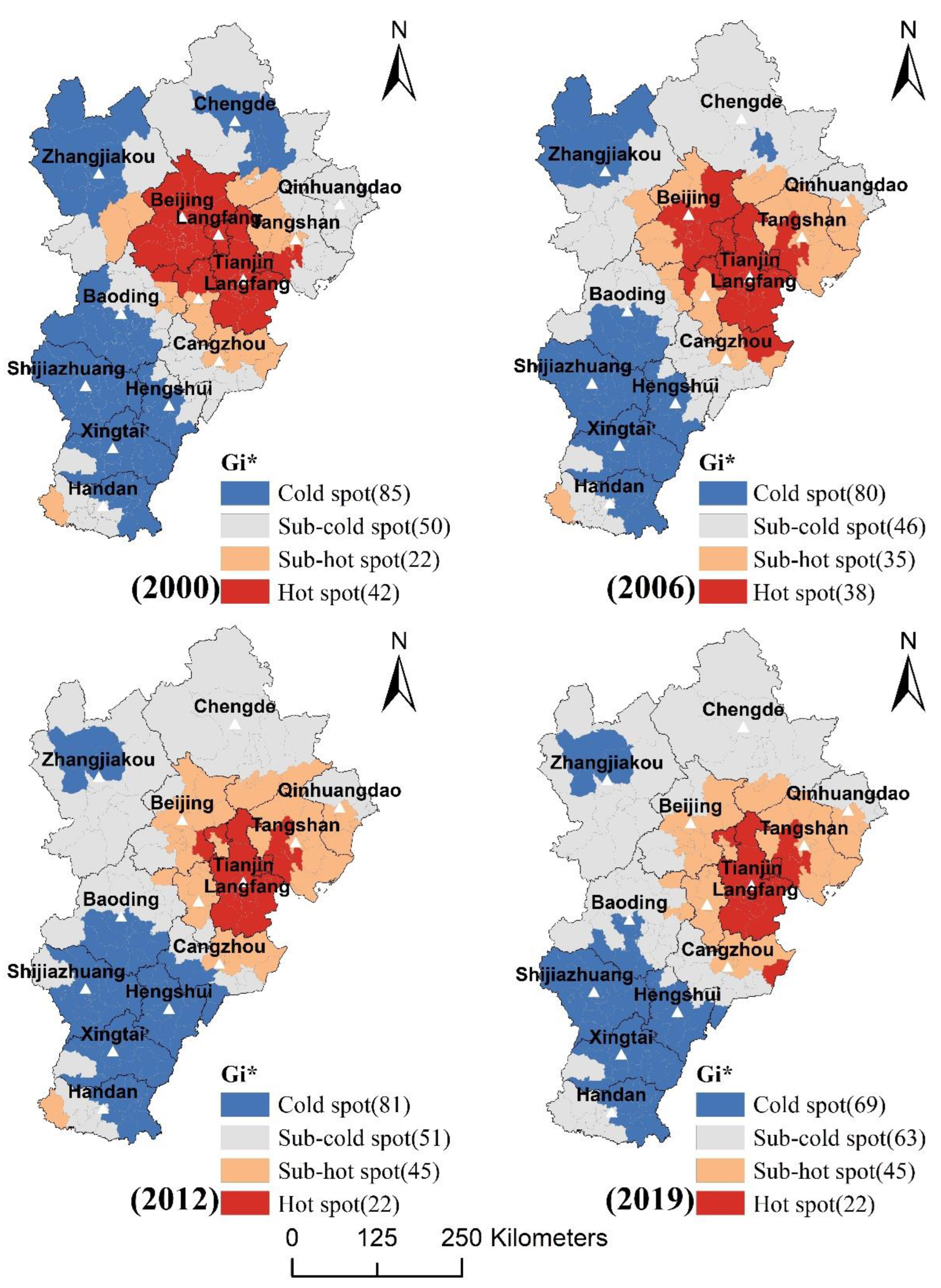
3.4.3. Hot Spots Analysis

The “Getis-Ord G*” indicator can be used to determine the spatially clustered locations of carbon emissions, which obey the standard normal distribution. It identifies statistically significant hot and cold spots using local General G index statistics given a set of weighted elements. When the “Getis-Ord G*” statistic passes the significance test and is positive, it means that carbon emissions are clustered in space, that is, hot spots; otherwise, it means discrete, that is, cold spots. The “Getis-Ord G*” can be expressed as follows:

$$G_i^{*}=\frac{{\displaystyle {\sum }_{j=1}^n{W}_{i,j}{x}_j}-\overline{X}{\displaystyle {\sum }_{j=1}^n{w}_{i,j}}}{\sqrt[S]{\left[n{\displaystyle {\sum }_{j=1}^n{w}_{i,j}{}^2}-{\left({\displaystyle {\sum }_{j=1}^n{w}_{i,j}}\right)}^2\right]/\left(n-1\right)}}$$

(15)

where $G_i^{\ast }$ is the Z-score, $W_{i,j}$ represents the spatial weight between space units $i$ and $j$ (adjacent is 1, non-adjacent is 0); $n$ is the number of space units, $x_j$ is the carbon emission value of the space unit; $\overline{X}$ represents the Mean, $S$ the standard deviation.

3.5. Spatial Econometrics Models

The modified STIRPAT stochastic extensible model based on IPAT proposed by York [31] was selected. Because of its flexibility, the model has been widely used in various fields [35,36].

CO₂ emission from energy consumption can reflect regional environmental pressure, so STIRPAT can better explore the driving factors of CO₂ emission. The formula is as follows:

$$I=a{P}^b{A}^c{T}^{d}e$$

(16)

where $I$ is an environmental factor; $P$ is the demographic factor, $A$ is the wealth factor, and $T$ is the technology factor; $a$ is a constant term; $e$ is an error; and $b$, $c$, and $d$ are indices that need to be evaluated. Logarithm transformation was performed on both sides of the model (16) at the same time, and it is expressed as:

$${\left(LnI\right)}_i=Ln{a}_i+b_i{\left(LnP\right)}_i+c_i{\left(LnA\right)}_i+d_i{\left(LnT\right)}_i+Ln{e}_i$$

(17)

where $i$ is the city $i$. The model was then extended based on the actual situation and existing data. $b_i$, $c_i$, and $d_i$ are elastic coefficients, which means that when $P$, $A$, and T change by 1%, $b_i$%, $c_i$%, and $d_i$% of $I$ will change respectively.

Table 3. STIRPAT model variable selection.

Variable	Factor		Symbol	Indicator	Unit
dependent variable	Environmental	CO2 emissions	CE	Urban carbon emissions	104 tons
independent variable	population factor	total population	p	Year-end total population	104 people
		Urbanization rate	UR	The proportion of urban population to total population	%
	Wealth factor	GDP per capita	PP	GDP per capita	Yuan
		Foreign investment	FAI	foreign investment	Ten thousand dollars
	technical factors	Secondary industry	TI2	Proportion of added value of secondary industry in GDP	%
		Industrial added value	LAV	Annual industrial added value	billion

shows the selected influencing factors. Since data on energy consumption per unit GDP and coal share were not available for cities in Hebei Province, these two terms were removed from the driving force analysis.

4. Results

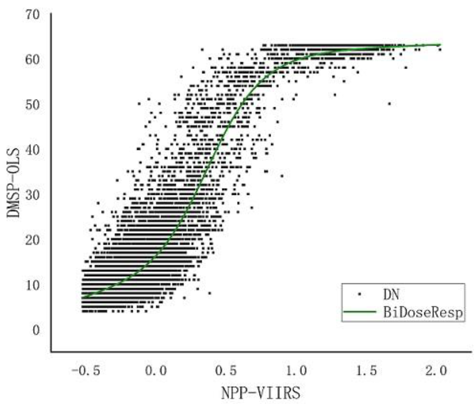
4.1. NSL Mutual Correction Results

The radiation characteristics of a certain area in Beijing-Tianjin-Hebei (including rural areas, urban areas and suburbs) in the nighttime light data and Google Earth image were selected for cross-sectional examination, as shown in Figure 5. It can be seen that the distribution of BDR (BiDoseResp) NPP (adjusted NPP-VIIRS) data is consistent with that of DMSP-OLS data. Figure 6 displays the nighttime stable light data (NSL) of the time series from 2000–2019 after the final continuous correction.

4.2. Accuracy Evaluation of CO₂ Emission Estimation

The bp-neural network was used as a tool to fit the relationship between CO₂ emissions and nighttime lighting data. The predicted value was then compared with the actual statistical value, and other functions were also used for comparison in order to verify the accuracy.

Table 4. Comparison of different function models.

	Model	R2	RMSE	RE
Beijing	Linear	0.5600	1186.443	0.0753
	quadratic fit	0.6129	1387.492	0.0902
	Exponential function	0.5231	2094.901	0.1294
	Power function	0.5934	1169.759	0.0754
	bp-neural network	0.9799	260.061	0.0158
Tianjin	Linear	0.8674	1741.121	0.0793
	quadratic fit	0.9327	2799.401	0.1281
	Exponential function	0.7828	2503.933	0.1081
	Power function	0.8483	1846.445	0.0768
	bp-neural network	0.9978	314.669	0.0146
Hebei	Linear	0.8497	9870.159	0.1334
	quadratic fit	0.9574	10281.500	0.1341
	Exponential function	0.7357	14073.120	0.1645
	Power function	0.8179	11682.530	0.1306
	bp-neural network	0.9963	2455.139	0.0269

shows the fitting results of different functional models on the DN value and CO₂ emissions. In comparison to other functional models, the BP-neural network was superior in every way. RMSE is the root mean square error, which measures the error rate of the regression model. The measurement’s accuracy is indicated by the average relative error (RE), which is the difference between the absolute error and the real value. It can be seen that the accuracy of fitting night light and CO₂ emissions by the BP-neural network was good, so the model can be used to fit CO₂ emissions in BTH.

4.3. Spatio-Temporal Dynamics of CO₂ Emissions

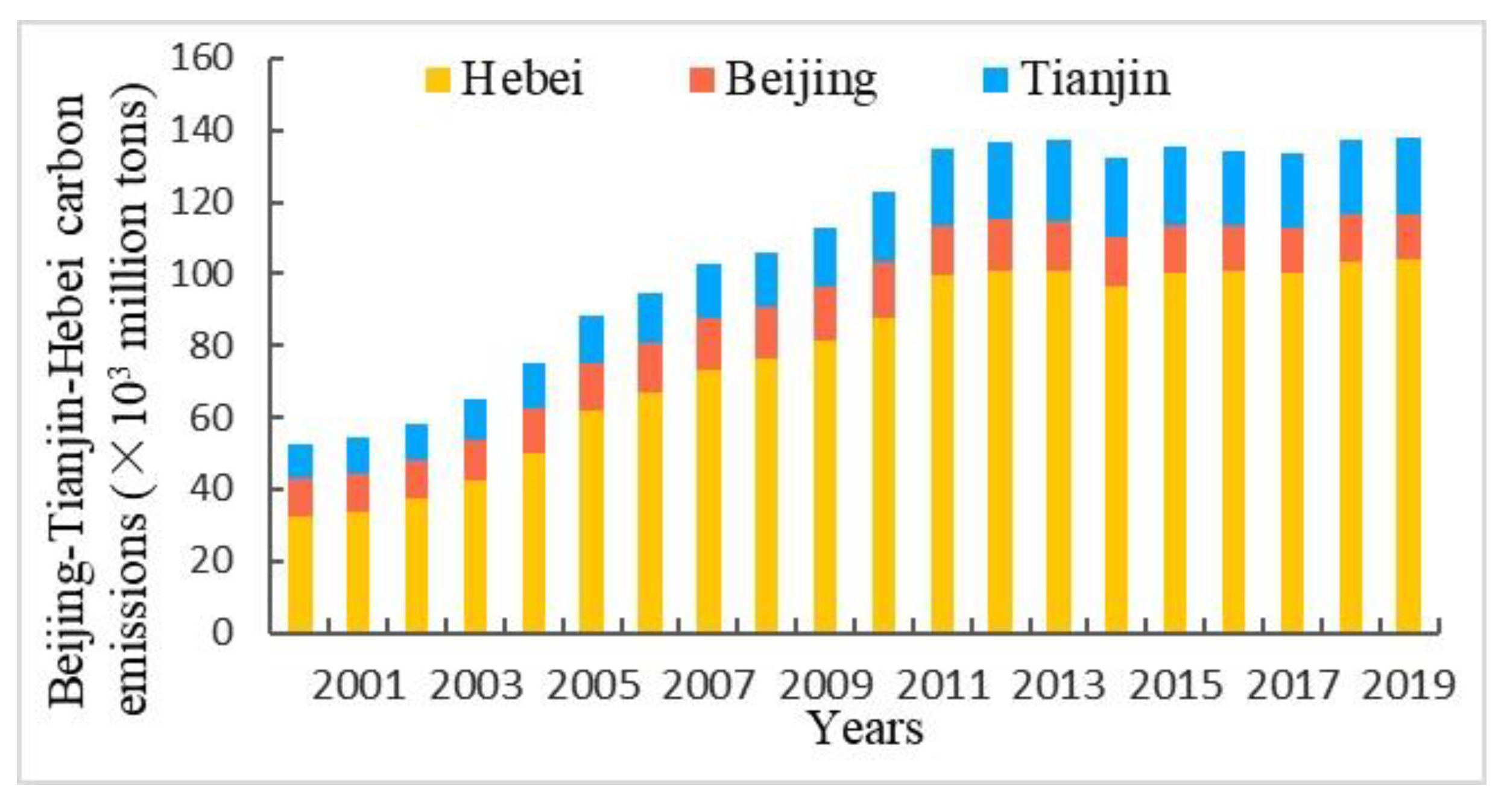
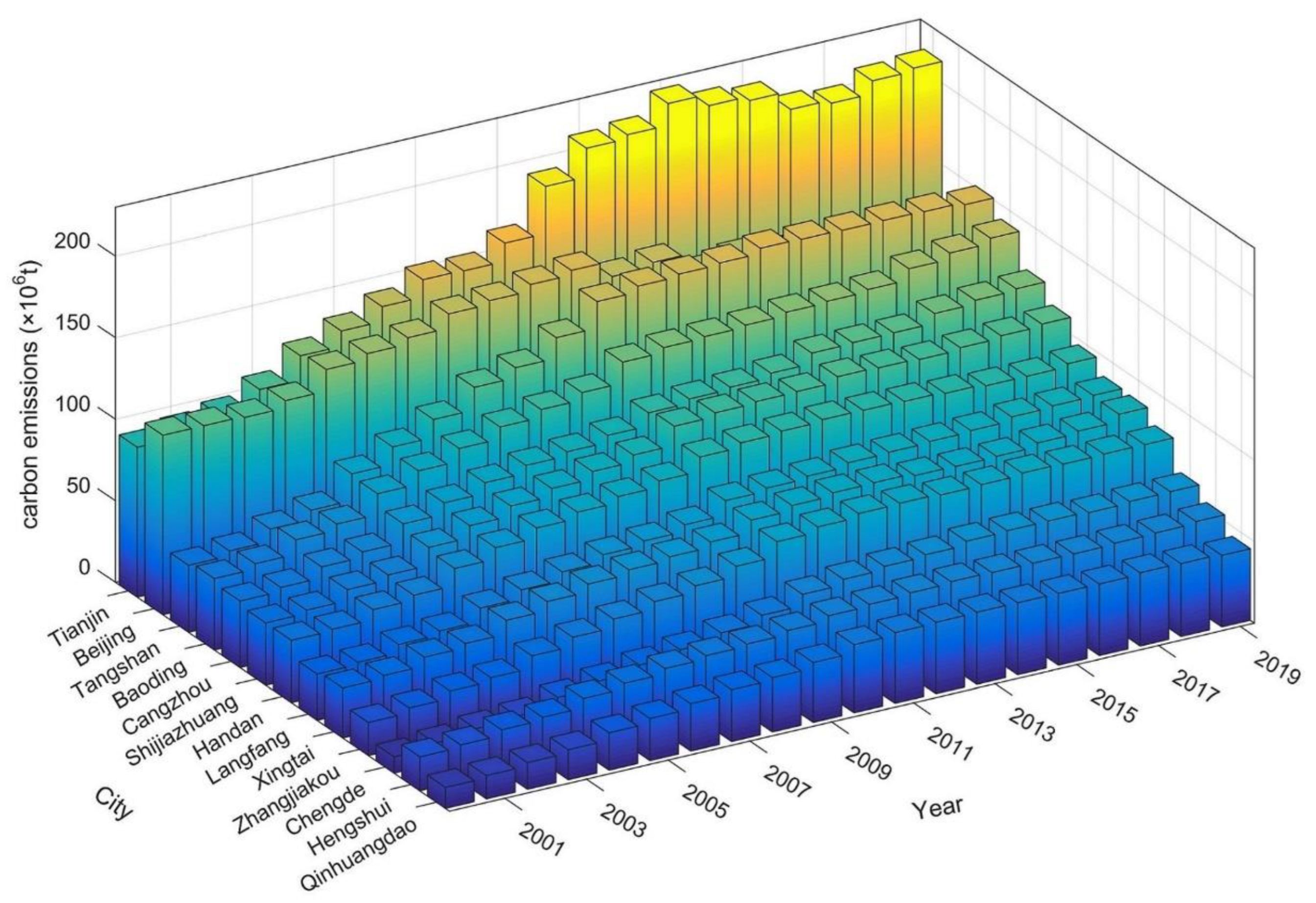
4.3.1. Temporal Variations

The total CO₂ emissions in BTH changed significantly, increasing from 525.26 million tons in 2000 to 1381.01 million tons in 2019, with an average growth rate of 4.952%. The upward trend from 2000–2012 gradually stabilized after 2012 and showed a downward trend in 2014, 2016 and 2017 (Figure 7). The CO₂ emissions of Hebei Province were basically consistent with the total CO₂ emission trend of Beijing-Tianjin-Hebei, from 61.5% in 2000 to 75.31% in 2017, and the growth rate has slowed since 2012.

At the municipal level, as shown in Figure 8, the CO₂ emissions of Tianjin have been significantly higher than those of other cities since 2010. Since 2004, the CO₂ emissions of Tangshan have steadily ranked first in Hebei Province, followed by Baoding. At the county level, the faster developing areas in the eastern portion of the Beijing-Tianjin-Hebei region were where CO₂ emissions were highest (Figure 9). Over the past 20 years, the CO₂ emissions in BTH cities have changed significantly. Since 2000, Tianjin’s Binhai New Area has consistently ranked first among all districts in terms of CO₂ emissions.

As shown in Figure 10, according to the county-level SLOPE results, the southern BTH region had the majority of the regions with significant tendencies. According to the classification standard, there were seven counties with a downtrend, concentrated in the center of Beijing and Tianjin, accounting for 0.89% of the total area; 96 slow growth areas; 69 medium growth areas; 24 faster growth areas; and three rapid growth areas, accounting for 71.79%, 22.95%, 4.28% and 0.084% of the total area, respectively. The places with faster growth were primarily spread out southeast of Beijing-Tianjin-Hebei, and the rapid growth areas were distributed in the Yingshouyingzi mining area of Chengde, the Hongqiao District, and the Heping District of Tianjin.

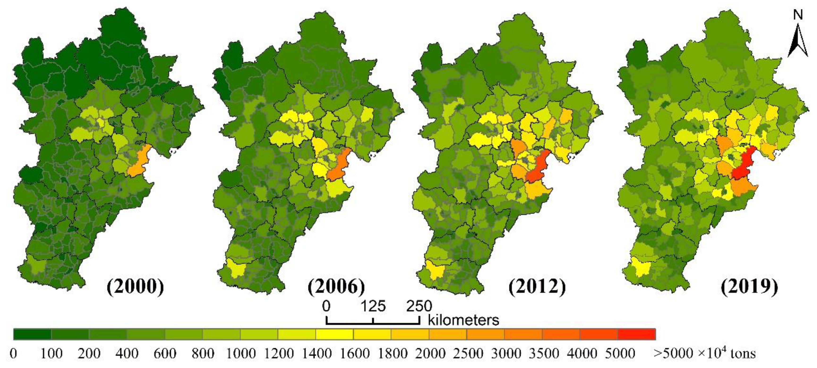
4.3.2. Spatial Variations

The global Moran’s I index was calculated in 2000, 2006, 2012 and 2019, which was 0.4501, 0.4023, 0.3938 and 0.3763 respectively (p < 0.01). This indicated that there was a positive correlation between county-level energy CO₂ emissions distribution in BTH during the past 20 years, and the correlation was gradually weakening. Over a 20-year period, CO₂ emissions became spatially dispersed.

Figure 11 shows that the southern and western counties of Hebei Province are the areas where the cold spot region mainly gathers. In 2019, the area of cold spot areas decreased, and the reduced cold spot areas were all converted into sub-cold spot areas. Beijing, Tianjin and surrounding areas were the main hot spots, and with the passage of time, the scope of hot spots gradually decreased and turned into sub-hot spots. The transformation of hot spots in Beijing was the most obvious, from the hot spots (16) in 2000 to the sub-hot spots (12) and sub-cold spots (4) in 2019, which indicates that the carbon reduction measures in Beijing have been very effective in recent years. Tianjin, as the economic center around the Bohai Sea, was also an international transportation hub, and has always remained in the hot spot.

4.4. Analysis of Driving Force

First, a Pearson analysis was performed on the data to remove insignificant factors and determine the influencing factors to be used. The least squares method was then used for regression to calculate the variance inflation factor (VIF) of the respective variables. The results demonstrated that most variables’ VIF values were above 10, which confirmed the existence of multicollinearity. To eliminate the effects of multicollinearity, the data was re-regressed using ridge regression analysis with biased estimation. It is an improved method based on the least square method. In order to obtain more realistic and reliable regression coefficients, it loses part of the information and reduces the accuracy [37]. When K = 0, it is the ordinary least squares estimate.

Because energy CO₂ emissions were normally distributed in Beijing from 2000–2019, only population and wealth factors were significantly correlated with energy CO₂ emissions in the Pearson test. To explore the causes of energy CO₂ emissions in Beijing, it was necessary to decompose the technical factors. Therefore, on the original basis, three independent variables of building, transportation and energy intensity were added. The formula can be expressed as:

$$LnI=Lna+bLnP+cLnA+dLnT+mLnU+nLnR+tLnE+Lne$$

(18)

where $U$ is the construction factor (CI), expressed by the number of construction enterprises; $R$ is the transportation factor (PC), expressed by the number of private cars (10,000 vehicles); $E$ is the energy intensity (GC), expressed by the unit GDP carbon dioxide consumption Quantity representation. Ridge regression analysis with biased estimation was conducted on the STIRPAT model, and the final regression results of Beijing are shown in

Table 5. Ridge Regression Estimation Results of Beijing.

Variables	Ln(UR)	Ln(FAI)	Ln(GC)	Ln(CI)	Ln(PC)	Constant	Sig F	R-Squared	K
coefficient	1.090 *** (0.258)	−0.029 * (0.016)	0.037 ** (0.013)	0.246 *** (0.044)	0.025 *** (0.007)	2.938 * (1.069)	0.0000	0.858	0.15

Note: “()” is the standard error; ***, **, * indicate significance at the 1%, 5% and 10% levels, respectively.

, and the results of other cities are shown in

Table 6. Ridge regression estimation results of Tianjin-Hebei.

	Tianjin	Shijiazhuang	Tangshan	Qinhuangdao	Handan	Xingtai
Ln(P)	0.249 *** (0.038)		1.711 *** (0.529)	1.941 *** (0.218)	0.323 *** (0.106)	0.436 ** (0.181)
Ln(UR)	1.418 *** (0.088)	0.572 *** (0.154)	0.406 *** (0.097)	0.258 ** (0.115)	0.282 *** (0.046)	0.339 *** (0.044)
Ln(PP)	0.132 *** (0.012)	0.092 ** (0.042)	0.149 *** (0.013)	0.151 *** (0.019)	0.129 *** (0.010)	0.134 *** (0.009)
Ln(FAI)	0.037 ** (0.017)		0.106 *** (0.017)	0.081 *** (0.019)	0.027 ** (0.012)
Ln(TI2)	0.265 *** (0.086)
Ln(LAV)	0.142 *** (0.012)	0.297 *** (0.055)	0.177 *** (0.020)	0.235 *** (0.029)	0.142 *** (0.015)	0.216 *** (0.021)
Constant	−2.32 *** (0.682)	3.731 *** (0.401)	−7.706 ** (3.447)	−7.598 *** (1.485)	3.136 *** (0.757)	1.999 * (1.125)
Sig F	0.0000	0.0000	0.0000	0.0000	0.0000	0.0000
R-squared	0.980	0.9541	0.963	0.939	0.943	0.961
K	0.03	0.05	0.26	0.24	0.4	0.25
	Baoding	Zhangjiakou	Chengde	Cangzhou	Langfang	Hengshui
Ln(P)	1.501 *** (0.223)	4.195 *** (0806)	2.425 *** (0.820)			1.409 *** (0.317)
Ln(UR)	0.258 *** (0.050)	0.432 *** (0.063)	0.639 *** (0.085)	0.634 *** (0.085)	0.741 *** (0.083)	0.330 *** (0.055)
Ln(PP)	0.115 *** (0.015)	0.142 *** (0.010)	0.166 *** (0.016)	0.199 *** (0.022)	0.114 *** (0.019)	0.100 *** (0.018)
Ln(FAI)	0.053 ** (0.025)	0.028 ** (0.013)			0.100 *** (0.026)
Ln(TI2)					0.412 *** (0.076)
Ln(LAV)	0.163 *** (0.030)	0.190 *** (0.019)	0.251 *** (0.029)	0.069 ** (0.029)	0.153 *** (0.022)	0.176 *** (0.034)
Constant	−5.056 *** (1.622)	−21.436 *** (4.898)	−11.487 ** (4.676)	4.236 *** (0.185)	1.089 ** (0.433)	−3.430 * (1.945)
Sig F	0.0000	0.0000	0.0000	0.0000	0.0000	0.0000
R-squared	0.933	0.943	0.988	0.985	0.990	0.900
K	0.33	0.48	0.08	0.04	0.05	0.37

Note: “()” is the standard error; ***, **, * indicate significance at the 1%, 5% and 10% levels, respectively.

.

Table 5 and Table 6 show that the significance test of 10% was passed by all of the chosen independent variables. Ridge regression results showed that R² was greater than 85%, F significance test Sig F = 0.0000 < 0.01, passed the significance level test. Therefore, it can be concluded that the relationship between CO₂ emissions and their respective variables in Beijing-Tianjin-Hebei cities can be well explained by models (17) and (18).

The urbanization rate (UR) promoted CO₂ emissions in all of the 13 cities, and the total population (P) of each city had a promoting effect on energy CO₂ emissions to a certain extent. The increase in the population and the migration of rural people to cities have led to the increase in urbanization rate and the change of industrial form, which are among the reasons for the increase in energy consumption. For Tianjin and some cities in Hebei, foreign investment (FAI) played a promoting role in CO₂ emission. Foreign investment promoted the level of industrialization and economic growth and improved the energy intensity of infrastructure construction and the mechanized production process. Therefore, a large amount of investment can produce higher CO₂ emissions [38].

The ratio of secondary industry to GDP (TI2) was only significantly correlated with CO₂ emissions in Tianjin and Langfang, indicating that the industrial structure had a stimulating effect on CO₂ emissions in these two cities during 2000–2019, and the effective adjustment of industrial structure could restrain CO₂ emissions. Except for Beijing, the increase of industrial added value (LAV) will lead to the increase of CO₂ emissions in the other 12 cities because the continuous increase of industrial added value will stimulate social demand and increase production intensity, resulting in more CO₂ emissions. For Beijing, urbanization rate (UR) was the most critical positive factor affecting its energy CO₂ emissions, and its elasticity value was the highest. For every 1% increase in the urbanization rate of Beijing, its energy CO₂ emissions will increase by 1.09%. Increased foreign investment (FAI) will curb CO₂ emissions in Beijing, as a large amount of investment is often accompanied by advanced technologies that use clean energy in the production process.

5. Discussion

5.1. Accuracy Assessment of CO₂ Emissions

The lack of energy statistics and inconsistent statistical standards in prefecture-level cities bring some difficulties to the analysis of the spatio-temporal CO₂ emissions dynamics. In this study, the method of using night light (NSL) to assess carbon dioxide proved to be effective. In order to assess the reliability of the findings, linear equations, quadratic terms, power functions and exponential functions were also used for comparison. Coefficient of determination (R²), relative error (RE), and root mean square error (RMSE) were used to assess the precision of the spatial distribution of CO₂ emissions. Among them, the coefficient of the neural network model is better than that of other function models, as shown in Table 4. However, this method is relatively dependent on the accuracy of NSL data. Due to some shortcomings of night light data, such as supersaturation and low accuracy, how to simulate CO₂ emissions more accurately through night light needs to be studied further.

5.2. The Role of Influencing Factors

The results of the spatial econometric model show that all the factors selected in this study have an effect on CO₂ emissions, especially the population factor, which is in line with the research findings of Wang [39]. Since 2010, there seems to be no direct correlation between Beijing’s carbon emission curve and its economic development curve, because the rapid economic growth accompanied by the use of advanced technology and clean energy has slowed the growth of CO₂ emissions [40]. The impact of foreign investment (FAI) on CO₂ emissions in the BTH region is different, with Beijing being negative and the other 12 cities being positive. For Beijing, with high GDP, advanced technologies can be transferred to domestic enterprises through foreign investment, and technology transfer can help domestic enterprises adopt new technologies and improve the energy efficiency of energy use [41]. For Tianjin and the cities in Hebei Province, a large amount of foreign capital inflow is responsible for the regional economic growth, but it inevitably leads to environmental pollution, thereby increasing carbon emissions [42]. Many scholars have analyzed different areas of the environmental stress factors, but most of the studies focused on large scale regions and ignore the regional internal differences, and this research solved this problem. However, the selection of influencing factors needs to be discussed further. Different scholars choose different influencing factors, which might have an effect on the study’s findings. At the same time, due to the high scalability of the STIRPAT model, the factors affecting energy consumption are complex. This study was conducted on the basis of available urban statistics, which did not include all of the influencing factors, especially the technical factor indicators. The establishment and improvement of the statistical index system of different scales will make the driving force research results more accurate. The detailed decomposition of the influence of each variable from a small-scale perspective is a direction for future research on regional environmental stress.

5.3. Compared with Previous Studies

Research on carbon emissions has become a hot topic in recent years. Previous studies have had a large scope and rarely involve city and county levels. For example, Shi [19] and Chen [43] chose China as their research area and studied China’s carbon emissions through single satellite data. The method proposed in this study has obvious advantages. By integrating two kinds of nighttime light data, long-term carbon emission data at different administrative levels in different cities can be obtained with certain accuracy. This study focused on the Beijing-Tianjin-Hebei region, which can more specifically analyze the driving principles behind the carbon emissions of cities and counties. Compared with previous studies, most of the carbon emissions and NSL fitting studies adopted the traditional linear method [22,23], in which Lv obtained the fitting RE of Beijing, Tianjin and Hebei to be 6.64%, 0.45% and 38.86%, respectively, while the fitting RE of this study was 1.58%, 1.46% and 2.69%, respectively. The errors of Beijing and Hebei are much smaller than the results of Lv. Therefore, the neural network method proposed in this study is superior to some other studies to a certain extent, and the final results are more accurate. Finally, in the analysis of driving factors, this study added some factors on the basis of previous studies. For example, traffic and building factors are added to the study of Beijing. Compared with the study of Wen [44], this research has a smaller scale and is accurate to each city, so it has more advantages.

6. Conclusions and Policy Implications

To some extent, the low-carbon development strategies formulated by the BTH can provide some references for other cities. However, the accurate analysis of small-scale regional carbon emissions is limited by the lack of statistical data in some cities. In order to resolve this issue, this work employed the integration of two kinds of nighttime lighting data to fit the CO₂ emissions of Beijing, Tianjin, and Hebei, and obtained the CO₂ emissions at different scales. Then, spatial analysis technology was used to examine spatial and temporal changes, and the driving force of CO₂ emissions was analyzed by the STIRPAT model with biased estimation ridge regression. The results show that the distribution pattern of energy CO₂ emission in Beijing-Tianjin-Hebei is “greater in the east than in the west” and is mainly concentrated in the eastern coastal cities and the cities with higher population density and higher GDP. There were variances in CO₂ emission levels across cities, and most displayed a pattern of first growing and then slowing down. With the exception of the Hongqiao District and Heping District, carbon emissions in central urban areas of Beijing and Tianjin showed a general decreasing trend. Tangshan, Baoding, Cangzhou and Shijiazhuang, which are the industrial, economic and political centers, are the areas with high carbon emissions in Hebei Province, and the CO₂ emissions of some counties in the south and northwest of Hebei Province show an increasing trend. The aggregation degree of carbon emissions in each district was weakened, and most of them showed a slowing trend.

According to the spatial econometric model’s findings, carbon emissions in Tianjin and Hebei are positively affected by population, wealth, and technology. In addition to the negative impact of foreign investment in Beijing, other factors are also positive. In the Beijing-Tianjin-Hebei region, population is the most significant factor determining CO₂ emissions. The weight of the same influence factor is different in different cities, and the difference is obvious within cities.

This study offers some policy suggestions for controlling CO₂ emissions based on the above discussion and conclusions. First, we should control the size of the population, optimize the population structure and alleviate the problem of high population density. At the same time, we should improve the quality of the population, and guide people’s environmental awareness and consumption concepts. Second, strictly controlling the approval of foreign investment and energy-intensive projects and raising the investment threshold to develop low-carbon industries can effectively control CO₂ emissions. Third, we should adjust the industrial structure and reduce the proportion of industries that consume large amounts of fossil energy. We need to encourage high-tech industries and establish a green and ecological industrial development model, especially in Tianjin, Shijiazhuang, Chengde and Langfang. For regions with underdeveloped economic development, such as Zhangjiakou and Hengshui, CO₂ emissions should be reduced by saving energy, improving energy utilization efficiency and actively cultivating low-carbon and green concepts. In addition, for Beijing, besides controlling the population size, the proportion of clean energy in total energy consumption can be increased, the consumption of fossil energy can be reduced, and public transportation can be advocated. Local governments should improve regional industrial guidance, encourage foreign investment in high-tech industries, and introduce resource-saving investments. At the same time, we need to develop low-carbon buildings and green buildings, and improve the relevant technical norms and standards.

References

1. Soytas, U.; Sari, R.; Ewing, B.T. Energy consumption, income, and carbon emissions in the United States. Ecol. Econ. 2007, 62, 482–489. [Google Scholar] [CrossRef]
2. Ciais, P.; Wang, Y.; Andrew, R.; Bréon, F.M.; Chevallier, F.; Broquet, G.; Nabuurs, G.J.; Peters, G.; McGrath, M.; Meng, W. Biofuel burning and human respiration bias on satellite estimates of fossil fuel CO2 emissions. Environ. Res. Lett. 2020, 15, 074036. [Google Scholar] [CrossRef]
3. Fang, C.; Wang, S.; Li, G. Changing urban forms and carbon dioxide emissions in China: A case study of 30 provincial capital cities. Appl. Energy 2015, 158, 519–531. [Google Scholar] [CrossRef]
4. Su, Y.; Chen, X.; Li, Y.; Liao, J.; Ye, Y.; Zhang, H.; Huang, N.; Kuang, Y. China’s 19-year city-level carbon emissions of energy consumptions, driving forces and regionalized mitigation guidelines. Renew. Sustain. Energy Rev. 2014, 35, 231–243. [Google Scholar] [CrossRef]
5. Apergis, N.; Payne, J.E. The causal dynamics between coal consumption and growth: Evidence from emerging market economies. Appl. Energy 2010, 87, 1972–1977. [Google Scholar] [CrossRef]
6. Guo, D.; Chen, H.; Long, R. Can China fulfill its commitment to reducing carbon dioxide emissions in the Paris Agreement? Analysis based on a back-propagation neural network. Environ. Sci. Pollut. Res. 2018, 25, 27451–27462. [Google Scholar] [CrossRef]
7. Wang, M.; Cai, B. A two-level comparison of CO2 emission data in China: Evidence from three gridded data sources. J. Clean. Prod. 2017, 148, 194–201. [Google Scholar] [CrossRef]
8. Mallapaty, S. How China could be carbon neutral by mid-century. Nature 2020, 586, 482–484. [Google Scholar] [CrossRef]
9. Yu, X.; Liang, Z.; Fan, J.; Zhang, J.; Luo, Y.; Zhu, X. Spatial decomposition of city-level CO2 emission changes in Beijing-Tianjin-Hebei. J. Clean. Prod. 2021, 296, 126613. [Google Scholar] [CrossRef]
10. Geng, Y.; Tian, M.; Zhu, Q.; Zhang, J.; Peng, C. Quantification of provincial-level carbon emissions from energy consumption in China. Renew. Sustain. Energy Rev. 2011, 15, 3658–3668. [Google Scholar] [CrossRef]
11. Müller, D.B.; Liu, G.; Løvik, A.N.; Modaresi, R.; Pauliuk, S.; Steinhoff, F.S.; Brattebø, H. Carbon emissions of infrastructure development. Environ. Sci. Technol. 2013, 47, 11739–11746. [Google Scholar] [CrossRef] [PubMed]
12. O’neill, B.C.; Dalton, M.; Fuchs, R.; Jiang, L.; Pachauri, S.; Zigova, K. Global demographic trends and future carbon emissions. Proc. Natl. Acad. Sci. USA 2010, 107, 17521–17526. [Google Scholar] [CrossRef] [PubMed]
13. Amaral, S.; Câmara, G.; Monteiro, A.M.V.; Quintanilha, J.A.; Elvidge, C.D. Estimating population and energy consumption in Brazilian Amazonia using DMSP night-time satellite data. Comput. Environ. Urban Syst. 2005, 29, 179–195. [Google Scholar] [CrossRef]
14. Sutton, P.C.; Taylor, M.J.; Elvidge, C.D. Using DMSP OLS imagery to characterize urban populations in developed and developing countries. In Remote Sensing of Urban and Suburban Areas; Springer: Berlin/Heidelberg, Germany, 2010; pp. 329–348. [Google Scholar]
15. Alahmadi, M.; Atkinson, P.M. Three-fold urban expansion in Saudi Arabia from 1992 to 2013 observed using calibrated DMSP-OLS night-time lights imagery. Remote Sens. 2019, 11, 2266. [Google Scholar] [CrossRef]
16. Gibson, J.; Olivia, S.; Boe-Gibson, G.; Li, C. Which night lights data should we use in economics, and where? J. Dev. Econ. 2021, 149, 102602. [Google Scholar] [CrossRef]
17. Chand, T.K.; Badarinath, K.; Elvidge, C.; Tuttle, B. Spatial characterization of electrical power consumption patterns over India using temporal DMSP-OLS night-time satellite data. Int. J. Remote Sens. 2009, 30, 647–661. [Google Scholar] [CrossRef]
18. Elvidge, C.D.; Ziskin, D.; Baugh, K.E.; Tuttle, B.T.; Ghosh, T.; Pack, D.W.; Erwin, E.H.; Zhizhin, M. A fifteen year record of global natural gas flaring derived from satellite data. Energies 2009, 2, 595–622. [Google Scholar] [CrossRef]
19. Shi, K.; Chen, Y.; Yu, B.; Xu, T.; Chen, Z.; Liu, R.; Li, L.; Wu, J. Modeling spatiotemporal CO2 (carbon dioxide) emission dynamics in China from DMSP-OLS nighttime stable light data using panel data analysis. Appl. Energy 2016, 168, 523–533. [Google Scholar] [CrossRef]
20. Zhang, X.; Wu, J.; Peng, J.; Cao, Q. The uncertainty of nighttime light data in estimating carbon dioxide emissions in China: A comparison between DMSP-OLS and NPP-VIIRS. Remote Sens. 2017, 9, 797. [Google Scholar] [CrossRef]
21. Zhao, J.; Chen, Y.; Ji, G.; Wang, Z. Residential carbon dioxide emissions at the urban scale for county-level cities in China: A comparative study of nighttime light data. J. Clean. Prod. 2018, 180, 198–209. [Google Scholar] [CrossRef]
22. Lv, Q.; Liu, H.; Wang, J.; Liu, H.; Shang, Y. Multiscale analysis on spatiotemporal dynamics of energy consumption CO2 emissions in China: Utilizing the integrated of DMSP-OLS and NPP-VIIRS nighttime light datasets. Sci. Total Environ. 2020, 703, 134394. [Google Scholar] [CrossRef] [PubMed]
23. Meng, L.; Graus, W.; Worrell, E.; Huang, B. Estimating CO2 (carbon dioxide) emissions at urban scales by DMSP/OLS (Defense Meteorological Satellite Program’s Operational Linescan System) nighttime light imagery: Methodological challenges and a case study for China. Energy 2014, 71, 468–478. [Google Scholar] [CrossRef]
24. Chen, J.; Gao, M.; Cheng, S.; Hou, W.; Song, M.; Liu, X.; Liu, Y.; Shan, Y. County-level CO2 emissions and sequestration in China during 1997–2017. Sci. Data 2020, 7, 1–12. [Google Scholar] [CrossRef]
25. Ang, B.W. The LMDI approach to decomposition analysis: A practical guide. Energy Policy 2005, 33, 867–871. [Google Scholar] [CrossRef]
26. Fan, Y.; Liu, L.-C.; Wu, G.; Wei, Y.-M. Analyzing impact factors of CO2 emissions using the STIRPAT model. Environ. Impact Assess. Rev. 2006, 26, 377–395. [Google Scholar] [CrossRef]
27. Kaika, D.; Zervas, E. The Environmental Kuznets Curve (EKC) theory—Part A: Concept, causes and the CO2 emissions case. Energy Policy 2013, 62, 1392–1402. [Google Scholar] [CrossRef]
28. Vaninsky, A. Factorial decomposition of CO2 emissions: A generalized Divisia index approach. Energy Econ. 2014, 45, 389–400. [Google Scholar] [CrossRef]
29. Brizga, J.; Feng, K.; Hubacek, K. Drivers of CO2 emissions in the former Soviet Union: A country level IPAT analysis from 1990 to 2010. Energy 2013, 59, 743–753. [Google Scholar] [CrossRef]
30. Ozcan, B.; Ulucak, R. An empirical investigation of nuclear energy consumption and carbon dioxide (CO2) emission in India: Bridging IPAT and EKC hypotheses. Nucl. Eng. Technol. 2021, 53, 2056–2065. [Google Scholar] [CrossRef]
31. York, R.; Rosa, E.A.; Dietz, T. STIRPAT, IPAT and ImPACT: Analytic tools for unpacking the driving forces of environmental impacts. Ecol. Econ. 2003, 46, 351–365. [Google Scholar] [CrossRef]
32. Ma, T.; Zhou, C.; Pei, T.; Haynie, S.; Fan, J. Responses of Suomi-NPP VIIRS-derived nighttime lights to socioeconomic activity in China’s cities. Remote Sens. Lett. 2014, 5, 165–174. [Google Scholar] [CrossRef]
33. Zhao, M.; Zhou, Y.; Li, X.; Zhou, C.; Cheng, W.; Li, M.; Huang, K. Building a series of consistent night-time light data (1992–2018) in Southeast Asia by integrating DMSP-OLS and NPP-VIIRS. IEEE Trans. Geosci. Remote Sens. 2019, 58, 1843–1856. [Google Scholar] [CrossRef]
34. Jeswani, R.; Kulshrestha, A.; Gupta, P.K.; Srivastav, S. Evaluation of the consistency of DMSP-OLS and SNPP-VIIRS Night-time Light Datasets. J. Geomat 2019, 13, 98–105. [Google Scholar]
35. Liddle, B.; Lung, S. Age-structure, urbanization, and climate change in developed countries: Revisiting STIRPAT for disaggregated population and consumption-related environmental impacts. Popul. Environ. 2010, 31, 317–343. [Google Scholar] [CrossRef]
36. Shahbaz, M.; Chaudhary, A.; Ozturk, I. Does urbanization cause increasing energy demand in Pakistan? Empirical evidence from STIRPAT model. Energy 2017, 122, 83–93. [Google Scholar] [CrossRef]
37. Meng, M.; Zhou, J. Has air pollution emission level in the Beijing–Tianjin–Hebei region peaked? A panel data analysis. Ecol. Indic. 2020, 119, 106875. [Google Scholar] [CrossRef]
38. Zhao, X.; Zhang, X.; Shao, S. Decoupling CO2 emissions and industrial growth in China over 1993–2013: The role of investment. Energy Econ. 2016, 60, 275–292. [Google Scholar] [CrossRef]
39. Wang, Z.; Yin, F.; Zhang, Y.; Zhang, X. An empirical research on the influencing factors of regional CO2 emissions: Evidence from Beijing city, China. Appl. Energy 2012, 100, 277–284. [Google Scholar] [CrossRef]
40. Liu, Z.; Guan, D.; Moore, S.; Lee, H.; Su, J.; Zhang, Q. Climate policy: Steps to China’s carbon peak. Nature 2015, 522, 279–281. [Google Scholar] [CrossRef]
41. Lee, J.W. The contribution of foreign direct investment to clean energy use, carbon emissions and economic growth. Energy Policy 2013, 55, 483–489. [Google Scholar] [CrossRef]
42. Peng, H.; Tan, X.; Li, Y.; Hu, L. Economic growth, foreign direct investment and CO2 emissions in China: A panel granger causality analysis. Sustainability 2016, 8, 233. [Google Scholar] [CrossRef] [Green Version]
43. Chen, H.; Zhang, X.; Wu, R.; Cai, T. Revisiting the environmental Kuznets curve for city-level CO2 emissions: Based on corrected NPP-VIIRS nighttime light data in China. J. Clean. Prod. 2020, 268, 121575. [Google Scholar] [CrossRef]
44. Wen, L.; Liu, Y. The Peak Value of Carbon Emissions in the Beijing-Tianjin-Hebei Region Based on the STIRPAT Model and Scenario Design. Pol. J. Environ. Stud. 2016, 25. [Google Scholar] [CrossRef]
Figure 1. Geographical location of Beijing–Tianjin–Hebei.
Remotesensing 14 04799 g001
Figure 2. Flowchart of Beijing–Tianjin–Hebei carbon emission technology.
Remotesensing 14 04799 g002
Figure 3. Image of the fitted Bidoseresp model in 2013.
Remotesensing 14 04799 g003
Figure 4. Three-layer BP neural network model.
Remotesensing 14 04799 g004
Figure 5. Profile distribution of radiation value of light images at different nights in 2013.
Remotesensing 14 04799 g005
Figure 6. Night light values before and after correction.
Remotesensing 14 04799 g006
Figure 7. Beijing–Tianjin–Hebei carbon emissions from 2000–2019.
Remotesensing 14 04799 g007
Figure 8. Beijing–Tianjin–Hebei municipal-level energy CO2 emissions from 2000–2019.
Remotesensing 14 04799 g008
Figure 9. County-level CO2 emissions in the Beijing–Tianjin–Hebei region in 2000, 2006, 2012 and 2019.
Remotesensing 14 04799 g009
Figure 10. 2000–2019 Beijing–Tianjin–Hebei energy CO2 emission trends.
Remotesensing 14 04799 g010
Figure 11. Aggregation of energy CO2 emissions in Beijing-Tianjin-Hebei in 2000, 2006, 2012 and 2019.
Remotesensing 14 04799 g011