Abstract
Error evaluation is essential for the improvement and application of the Integrated Multi-satellitE Retrievals for the Global Precipitation Measurement (IMERG) Version 06 daily precipitation estimates, including early-, late-, and final-run products (IMERG-DE, IMERG-DL, and IMERG-DF, respectively), especially for summer precipitation in complex topographical areas. However, many existing works mainly focus on comparing the error statistical metrics of precipitation estimates, but few further analyze the internal relationships between these error statistics and geographical features. Therefore, taking Sichuan Province of China as a case study of the complex topographic and mountainous area, we adopt statistical metrics, error decomposition schemes, systematic and random error separation models, and regression methods to analyze the relationships between the spatial distribution of IMERG summer precipitation error metrics and geographical features. These features include longitude, latitude, distance from Sichuan Basin edge (DFBE), digital elevation model (DEM), normalized difference vegetation index (NDVI), slope, aspect, and topographic position index (TPI). The results show that: (1) DEM and DFBE are the two most important geographical features affecting the spatial distribution of error metrics, while both aspect and TPI have negligible effects on these metrics; (2) the variations in DEM, DFBE, and latitude have the negative relationships with error metrics; (3) longitude and DFBE do not have a direct impact on the errors, but indirectly affect the precipitation errors through the changing DEM; (4) slope shows a strong negative correlation with hit bias, and its increase significantly amplifies the sensitivity of systematic errors of hit bias from IMERG-DE and DL; and (5) the high detection probability and small missed precipitation error of the three IMERG estimates are virtually unaffected by changes in geographical features.
1. Introduction
Summer precipitation events related to catastrophic natural disasters such as floods, mudslides, and landslides frequently occur in western China, especially in the Sichuan Province with complex topographical conditions [1,2]. These precipitation events seriously affect the safety of local residents’ lives and property, and directly hinder the rapid development of the regional economy. Therefore, accurate observations of precipitation are essential for warning against and predicting geological disasters, and they can also provide more effective coping strategies for the management of urban water resources and the handling of other related emergencies [3].
At present, rain gauges suffer from representativeness issues when estimating precipitation over complex terrain due to the sparse and uneven distribution of the sites. Ground-based radars are inevitably affected by electromagnetic beam blockage and anomalous propagation errors in mountainous regions [3,4]. In addition, the limited working hours make it impossible for airborne radar to become a conventional way of precipitation observation. Therefore, satellite-based remote sensing may be the most reliable and stable way to obtain high spatiotemporal resolution precipitation in mountainous and complex topographical areas [5,6].
With the vigorous development of remote sensing technology, the quality of satellite-based precipitation estimates (SPEs) is constantly improving. Nowadays, by combining as many satellite and ground observations as available, the quasi-global SPEs are becoming more plentiful, such as the Global Precipitation Climatology Project (GPCP) [7], the Precipitation Estimation from Remotely Sensed Information using Artificial Neural Networks (PERSIANN) [8], the Climate Prediction Center MORPHing technique (CMORPH) [9], the Tropical Rainfall Measuring Mission Multi-satellite Precipitation Analysis (TRMM-TMPA) [10], the Global Satellite Mapping of Precipitation (GSMaP) [11], and the Integrated Multi-satellitE Retrievals for Global Precipitation Measurement (GPM-IMERG) [12]. Among them, the GPM-IMERG, which adopts the dual-frequency active microwave radar technology and is produced by the National Aeronautics and Space Administration (NASA), has wider spatial coverage, finer spatiotemporal resolution, and higher measurement accuracy, and it shows great application potential in the field of meteorology and hydrology. In addition, depending on the complexity of the generation strategies, IMERG provides three products, including the “Early” run (IMERG-E), “Late” run (IMERG-L), and “Final” run (IMERG-F) estimates, which may have different error characteristics. Therefore, a comprehensive data quality assessment and in-depth error sources exploration are necessary and have great practical value before applying the IMERG estimates.
At this stage, many researchers have done a lot of work for the analysis of IMERG errors. By summarizing these works, we find that:
- (1)
- Most studies use conventional statistical metrics to evaluate the overall performance of IMERG estimates, and ultimately attribute the errors to the features such as precipitation intensity and mechanism, solid precipitation, and high altitude [13,14,15,16,17]. However, this research seldom systematically analyzes the error sources and investigates the relationships between the characteristics of errors and the distributions of geographical features.
- (2)
- Some existing studies have proved that the data quality of IMERG varies greatly in different regions and seasons, and the lack of accuracy problem arises in IMERG summer precipitation estimates over the high latitude and elevation regions [5,16,18,19,20,21]. However, few studies have been carried out on the errors of IMERG summer estimates in Sichuan Province, which is one representative of the complex topographical areas and an ideal model for studying the influence of topography on precipitation.
- (3)
- Many studies have reported some potential influence factors of precipitation observation, such as complex precipitation mechanism [13], high elevation [15], high latitude [22], multiple-phase precipitation [14], complex topography [23], temperature [24], bodies of water [5], and so on. At the same time, it should be noted that topographical conditions have been shown to prominently affect the quality of remote sensing data [5,23,25,26,27,28,29,30]. Regrettably, the varieties of geographical features considered in this type of research are very limited.
Based on the above analysis, more attention should be paid to more geographical features, which may cause severe geometric errors and systematic errors in observations [27]. Therefore, in this study, focusing on the relationships between various geographical features and precipitation estimation errors, we conduct a more complete error analysis of IMERG summer estimates in the complex topographical region. The features are as follows: (1) more types of IMERG estimates: IMERG-E, L, and F; (2) more comprehensive error analysis methods, including not only conventional statistical metrics, but also error decomposition scheme, systematic and random errors separation strategies; (3) more typical complex topography: Sichuan Province in western China is selected as the study area; (4) more kinds of geographical features: longitude, latitude, distance from Sichuan Basin edge, digital elevation model, normalized difference vegetation index, slope, aspect, and topographic position index (hereafter called Lon, Lat, DFBE, DEM, NDVI, Slope, Aspect, and TPI, respectively).
Therefore, taking the Sichuan Province as a case of the complex terrain and mountainous area, we conduct an in-depth analysis of the relationships between the errors of the three IMERG estimates and the variations in geographical features. This research yields less ambiguous assessment and more valuable insights for data producers to infer the origin of the errors, allowing users to understand the strengths and weaknesses of IMERG estimates and choose high-quality products.
The remaining sections of the paper are structured as follows: The study area, GPM IMERG precipitation estimates, ground reference, and topographical data sets are introduced in Section 2. The statistical metrics, decomposition scheme, systematic and random error separation models, and regression method are described in Section 3. Section 4 presents the spatial characteristics of statistical error metrics, independent error components, and systematic and random errors in the three IMERG estimates, and the influence patterns of seven geographical features on precipitation estimate errors. Finally, the discussion and conclusions are provided in Section 5 and Section 6.
2. Study Area and Data Sets
2.1. Study Area
Sichuan Province, located in the southwest of China (26°03′–34°19′N, 97°21′–108°12′E), is the transition zone between the Qinghai–Tibet Plateau and the eastern plain of China, and has a total area of about 4.86 × 10⁵ km2. The geomorphology and topography in its territory are very complex and diverse, mainly composed of mountains, hills, plains, basins, and plateaus. Besides, its elevations span a broad range from 100 m to 7000 m, showing the characteristics of being high in the west and low in the east (see Figure 1a). The unique geographical location of Sichuan Province makes precipitation events mostly occur in summer [31,32], and the diversity of terrain expands the distribution range of geographical factors (such as Lon, Lat, DFBE, NDVI, DEM, Aspect, Slope, and TPI, etc.), as shown in Figure 1b–f. In addition, studies have shown that geographic factors have a great influence on the intensity and spatial distribution of precipitation [33,34], and are closely related to the precipitation measurement errors of satellites or other remote sensing instruments [25,26,27]. Therefore, Sichuan Province, as a representative of the complex topographical area, is an ideal area to study the relationships between geographical features and summer precipitation errors.
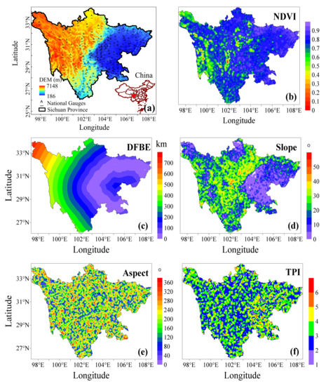
Figure 1.
(a) Geographical location and digital elevation model (DEM) of the study area, and the spatial distributions of national gauges stations (black pentagrams); (b–f) represent the distributions of NDVI, DFBE, slope, aspect, and TPI over Sichuan Province, respectively.
2.2. Data Sets
2.2.1. GPM IMERG Precipitation Estimates
Taking global precipitation observation as a mission, the GPM Core Observatory carrying the first spaceborne dual-frequency phased-array precipitation radar (13 and 35 GHz) and a conical-scanning multichannel microwave imager (10–183 GHz) was deployed by NASA and the Japan Aerospace Exploration Agency (JAXA) on 28 February 2014 [3]. The GPM mission provides four levels of data products, of which IMERG is the level 3 product with relatively fine spatiotemporal resolution (0.1° × 0.5 h). IMERG provides three types of precipitation estimates with different delay times: IMERG-E (4 h latency), IMERG-L (12 h latency), and IMERG-F (3.5 months latency) according to the complexity of the product generation strategy. For instance, instantaneous PMW precipitation estimates are only propagated forward in time by the morphing scheme of IMERG-E, whereas both forward and backward morphing schemes are employed in IMERG-L and IMERG-F [35]. Besides, IMERG-E and IMERG-L are calibrated by using the Global Precipitation Climatology Project (GPCP) climatological data, while IMERG-F combines the Global Precipitation Climatology Centre (GPCC) monthly precipitation analysis for bias correction. Therefore, IMERG-F is supposed to have better data quality than the other two IMERG estimates. At present, IMERG estimates have been updated to the latest Version 06B.
In this study, to facilitate the errors analysis of summer precipitation, we employed the IMERG V06B daily estimates, including early-, late-, and final-run products (IMERG-DE, IMERG-DL, and IMERG-DF, hereafter called DE, DL, and DF, respectively). The IMERG daily estimates are produced by resampling the half-hourly data to daily resolution in accord with the period of 000000-235959 UTC (universal time coordinated), and the unit of mm/day. The research period is from June to August of 2016–2020. All the IMERG data used in this paper are accessible on the PMM website (https://disc.gsfc.nasa.gov/datasets/GPM, accessed on 19 January 2022).
2.2.2. Ground Reference Data Sets
Ground reference data with high spatiotemporal resolution (0.1° × 1.0 h), namely the China Merge Precipitation Analysis (CMPA) version 1.0, is developed by the National Meteorology Information Center of the China Meteorological Administration (CMA) and can be obtained from the website of the CMA (http://data.cma.cn, accessed on 11 March 2021). The CMPA is generated by combining the hourly measurements from >30,000 ground rain gauges in China and the CMORPH (CPC MORPHing technique) satellite precipitation estimates using a climatology-based probability density function-optimal interpolation algorithm [36]. Besides these, a series of quality control measures, such as limits on climatological and regional precipitation extremes, and checks on data’s temporal and spatial consistency, are used to generate high-quality data. Therefore, CMPA is often used as the benchmark in related studies to evaluate the accuracy and precision of IMERG estimates [30,37,38]. Even so, some measurement errors are also unavoidable in high-altitude or high-latitude regions, such as wind-induced undercatch and wet/evaporation loss. Particularly, the undercatch errors will lead to a severe underestimation of precipitation due to the effect of wind and snowfall [39]. To resolve this problem, the correction schemes and some conclusions in Tang [39] and Ma et al. [40] are used to reduce this type of error. In this paper, the time of CMPA is UTC and the daily products are generated by accumulating the hourly data over 24 h.
2.2.3. Topographical Data Sets
The Shuttle Radar Topography Mission (SRTM) is jointly measured by NASA and National Geospatial-Intelligence Agency (NGA) [41]. SRTM data can be divided into SRTM1 and SRTM3 according to the different spatial resolutions, which correspond to 30 m and 90 m respectively, and the latter are the original data for generating the DEM, DFBE, Slope, Aspect, and TPI. In addition, the spatiotemporal resolutions of NDVI are 250 × 250 m and 5-day. All topographical data sets used in this research can be downloaded from the website of Geospatial Data Cloud (http://www.gscloud.cn, accessed on 17 January 2022). The generation of DFBE also requires the boundary information of the Sichuan Basin, which is extracted using ArcGIS software. For a particular grid point, its DFBE value is the minimum distance between this point and all points on the edge of the Sichuan Basin. The slope is the rate of change in the height of the ground area, and it is in the range of 0 to 90 degrees. Aspect refers to the orientation of the terrain slope, and it varies from 0 to 360 degrees. Generally, they are generated by fitting conicoid [42]. Specifically, the target point is first set as the center of a 3-by-3 grid, and then the elevation gradients of the target point in the horizontal and vertical directions (record as and , respectively) are calculated. Finally, the basic equations used to calculate the slope and aspect of the target point (record as and , respectively) are: , . Additionally, TPI represents the position of the target on the slope, such as ridge, upper slope, middle slope, flat slope, lower slope, and valley, corresponding to a value from 1 to 6. It is generated after comprehensively considering the difference between the altitude of the target point and the average altitude of the surrounding points, as well as the slope information. TPI is a parameter to describe the topography and has considerable significance in the classification of landforms [43]. The selection of Lat and DEM is based on the conclusions of previous studies [5,15,22]. The DFBE indicates the transfer distance from the Sichuan Basin to other areas, which further represents the transformation and reaching difficulties of moisture [44]. The other geographical features are chosen by preliminary results and reasonable deduction from our ongoing research. It is noteworthy that to obtain a data set with 0.1° × 0.1° spatial resolution, ArcGIS software is used to reduce the resolution of the original data sets.
3. Methodologies
3.1. Traditional Statistical Error Metrics
In the general assessment of data quality, continuous traditional statistical metrics, such as correlation coefficient (CC), relative bias (RB), and their average values are commonly used. Specifically, CC describes the agreements between the estimates and true measurements, and RB can reflect the degree of overestimation or underestimation of estimates. Meanwhile, contingency statistical metrics, including the probability of detection (POD), the false alarm ratio (FAR), and their average values are frequently used metrics when evaluating the precipitation detection capabilities of IMERG. The POD reflects the probability that precipitation is correctly detected by IMERG among all the real precipitation events, while the FAR represents the fraction of unreal events among all the precipitation events. In practice, the threshold of the daily precipitation events is set as 1.0 mm/day [45]. The related equations are listed in Table 1.

Table 1.
Traditional error statistical metrics.
3.2. Independent Error Components
For better tracking the sources of IMERG errors, an error decomposition scheme proposed by Tian et al. [45] can be used to decompose the total errors (TE, its mean value being ME) into three independent error components, including the bias of hit precipitation (HB), missed precipitation (MP), and false precipitation (FP). HB represents the difference between the estimates and true values when precipitation events are correctly detected by both IMERG and CMPA. MP indicates the errors due to IMERG not detecting the true precipitation events. FP denotes the errors of false precipitation only detected by IMERG.
For a given precipitation field , its binary mask can be obtained by a fixed threshold,
For and , their binary masks are and , respectively. Therefore, the hit, missed, and false precipitation masks are , , and respectively, and can be defined as follows:
where and are the Boolean complements of and , respectively. Thus, the TE, HB, MP, and FP are defined as:
Besides, the relationship between the three independent components (HB, MP, and FP) and TE is .
Given this, the scheme of decomposing the TE into HB, MP, and FP is useful for algorithm developers looking to trace the sources of errors and improve the quality of IMERG.
3.3. Systematic and Random Errors
For the IMERG summer precipitation over Sichuan, HB is the leading contributor to TE according to our previous study [21]. So, it is necessary to conduct in-depth research on the HB to separate the systematic and random errors. Of course, uncertainty quantification relies on the underlying error model [46]. Tang et al. [47] found that the multiplicative model is a better choice for quantifying the errors in daily precipitation measurements. In addition, Willmott [48] and AhaKouchak et al. [49] suggested that the mean square error () of precipitation can be divided into systematic errors () and random components () as .
where is defined in the form of the multiplicative model as
The Equation (6) is converted into the new expression of (7) after a natural logarithm transformation:
where and are the offset and scale parameters, respectively, and is the residual. The a and b parameters can be estimated easily by using the ordinary least-squares (OLS) method. The specific calculation process is shown in Equations (8) and (9), where n is the length of the sequence.
Defining , , and , the systematic errors () and random errors () can be written as
It is noteworthy that Equations (10) and (11) indicate that systematic and random errors are presented as a percentage of total errors in this study, and the sum of and is 100%.
3.4. Regression Analysis
Regression analysis is mainly used to study the relationships between error objectives (e.g., statistical error metrics, independent error components, systematic and random errors) and various geographical features, focusing on analyzing the contribution rate of each geographical feature to the errors, and then determining the principal determinants of the errors [30]. Note that geographical features as variables, including Lon, Lat, DFBE, DEM, Slope, Aspect, and TPI, have a commonality that they do not change with the variations in time and precipitation intensity. For evaluating the accuracy of the regression model, an important index, namely the coefficient of determination (), should be calculated first before using the model. This index is the goodness of fit in this regression model, and varies between 0 and 1 (best as 1).
where the subscript “N” indicates normalization, represents the normalization of error objectives, and and are the standardized regression coefficient and residual, respectively. and are the estimated and average values of , respectively.
Note that the standard regression coefficients are taken as absolute values, divided by the sum of all coefficients, and finally shown in the form of the percentages in this study. Therefore, the sum of all coefficients after processing is 100%. The purpose of this processing is to focus on the weight distributions of geographical features in .
4. Results
4.1. Traditional Statistical Error Metrics
For all traditional statistical error metrics, the values of the regression model are between 0.55 and 0.73. Note that the CC has the highest values, exceeding 0.65. These results indicate that the traditional statistical error metrics and geographical features have obvious, even significant, linear relationships. Subsequently, the regression analysis is used to calculate the correlation between statistical error metrics and geographical features, and the results are shown in Figure 2. Figure 2 shows that for any statistical metrics, longitude, latitude, DFBE, DEM, and slope are the main contributors to the errors because the sum of their weights exceeds 94%, which means that NDVI, aspect, and TPI have a nonlinear relationship with the geographical features.
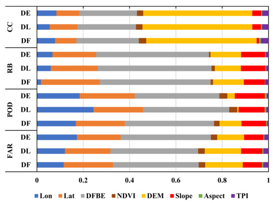
Figure 2.
The weight distribution of regression coefficients is based on statistical error metrics.
For all the IMERG estimates, DEM is the most sensitive feature for the CC (weighs around 0.47), followed by DFBE and Lat (weighs about 0.26 and 0.10, respectively). Meanwhile, these three geographical features, which have similar weight distributions, are also the most important sensitive sources of the RB and the FAR, among which DFBE becomes the most important contributor (weights > 0.38), followed by Lat and DEM (weights are about 0.2 and 0.14, respectively). The POD is mainly determined by DFBE, Lat, and Lon, with weights of 0.38, 0.22, and 0.17, respectively. The significant differences in the DEM weights in the POD between NRT IMERG daily estimates and IMERG-DF are that the weight of the former is only around 0.01, while the weight of the latter is as high as 0.11. In addition, we also notice that the influence of slope on the RB, POD, and FAR is much larger than that on the CC, while DEM shows a much greater impact on the CC than the impact shown by other metrics.
Figure 3 shows the spatial distributions of the statistical metrics for all three IMERG estimates. As shown in Figure 3, all three IMERG estimates exhibit similar spatial distributions for the same error statistical metric, but there are still some differences in detail. For the plateau region located in western Sichuan, severe overestimation of precipitation in the north area is quite common among the three IMERG estimates, while for other regions of the plateau, NRT IMERG and IMERG-DF only slightly underestimate and overestimate precipitation, respectively (see Figure 3d–f). IMERG-DF has better performance on CC but with relatively higher RB than that of NRT IMERG for the basin area in eastern Sichuan (see Figure 3a–f).
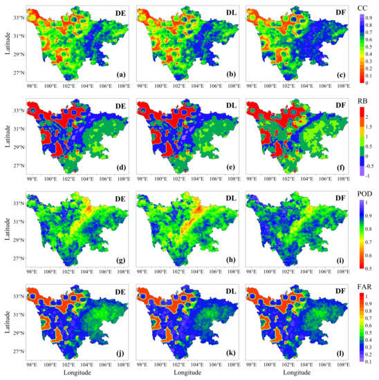
Figure 3.
Spatial distributions of the statistical metrics for the IMERG-DE (left column), DL (middle column), and DF (right column): (a–c) CC, (d–f) RB, (g–i) POD, (j–l) FAR.
In terms of the performance detecting precipitation, the three IMERG estimates have high POD and low FAR in most areas of Sichuan [see Figure 3g–l], which indicates that they have a good ability in enhancing precipitation capture. Among these, IMERG-DF performs the best. However, we find that abnormally high POD and FAR coexisted in the northern part of the plateau, which illustrates that IMERG has severely over-captured the precipitation in this region.
In addition to the plateau and basin areas, the region at the boundary between the plateaus and basins is also worthy of critical attention. All three IMERG estimates show abnormally low values on the RB, POD, and FAR for the heavy and extreme rainfall events that often occur in this region, which implies that the estimation accuracy and detection ability of IMERG are greatly limited by the topographical environment there. The reason may be that convective precipitation is easily generated in this unique topographical environment, but its spatial scale is much smaller than the resolution of remote sensors, which will cause the peak level of the precipitation intensity to be smoothed, leading to a significant reduction in the data quality of IMERG. Additionally, it is noteworthy that we found the three geographical features (NDVI, aspect, and TPI) have almost no intrinsic relationship with the error of precipitation, thus the results related to them are not presented in the following content.
The longitude, latitude, DFBE, DEM, and slope ranges are divided into many statistical intervals with steps of 0.5°, 0.5°, 50 m, 500 m, and 10°, respectively. Then, their average values are calculated in each statistical interval, and the statistical results are shown in Figure 4. Figure 4 shows that the curves for the IMERG-DE with any geographical feature are found to coincide with those of the IMERG-DL, and are very similar to the curves of IMERG-DF in terms of CC, POD, and FAR. For RB, curves of NRT IMERG daily estimates and IMERG-DF reveal a noticeable gap among the low longitude and high-latitude areas, DFBE, and DEM. The variation trend of geographical features makes the curve of POD little change, but the curves of other statistical metrics show large fluctuations.
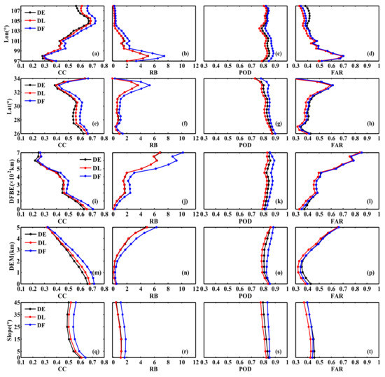
Figure 4.
The distributions of statistical metrics with different geographical features for the IMERG-DE, DL, and DF estimates. From left to right, four columns represent the CC (a,e,i,m,q), RB (b,f,j,n,r), POD (c,g,k,o,s), and FAR (d,h,l,p,t). From top to bottom, the five rows represent longitude (a–d), latitude (e–h), DFBE (i–l), DEM (m–p), and slope (q–t), respectively.
In terms of longitude trends, we noticed the obvious shift in the curves of all the statistical metrics occurs around 98°E, except for POD. More specifically, the data quality tends to degrade (with CC decreasing and RB, FAR increasing) with increasing longitude until 98°E, then gets better quickly. In conclusion, for most regions, the increase in longitude has a positive effect on the improvement of IMERG data quality (see Figure 4a–d).
Regarding latitude trends, we found that the curves of almost all the statistical metrics except POD change radically near the latitudes 27.5°N and 33°N, which are located at the southernmost and northern borders of the Sichuan Basin. From 27.5 to 30.5°N, the data quality degrades slowly (CC decreases while RB and FAR increase), followed by a sharp deterioration until 33°N. Conversely, these statistical metrics only get better with increasing latitude in small areas at both ends of the region (<27.5°N and >33°N). This suggests that the data quality of IMERG reveal negatively correlated with the latitude in most regions (see Figure 4e–h).
For DFBE, the CC, RB, and FAR metrics remain stable when DFBE is in the range of 200–350 km but deteriorate rapidly as DFBE increases in other ranges. According to Figure 3, the area with DFBE < 200 km includes the inner and outer edges of the Sichuan Basin, where IMERG estimates significantly overestimate and underestimate the precipitation, respectively. Therefore, the slightly higher or lower estimation of precipitation in this region is attributed primarily to the mutual cancellation of overestimation and underestimation, and the high FAR in IMERG estimates should be borne by the inner edge of the basin (see Figure 4j,l). Furthermore, in the area with DFBE > 200 km, the changes in statistical metrics are completely determined by the performance of IMERG in the western Sichuan plateau. The shift of the curve around 500 km (located at the westernmost end of the plateau) should be attributed to the instability of data quality caused by the sparse ground observation networks.
With the increase in DEM, the CC and RB remain stable inside 1.5 km and then deteriorate above 1.5 km. 1.5 km is also a cut-off point of the FAR, and the FAR decreases slowly and then increases rapidly inside or outside of the cut-off point. Meanwhile, we note that the data quality of IMERG is quite poor (CC < 0.5, RB > 200%, and FAR > 0.5) more than 3 km above altitudes, which reminds us that IMERG is no longer suitable as a dataset to analyze and estimate the precipitation in this region.
Furthermore, it is also found that, with the increase in slope, the fluctuations of all statistical metrics are smaller than that with other geographical features. The trend of statistical metrics reveals that the increase in slope slightly reduces the overestimation error of IMERG estimates and weakens the positive correlation with the precipitation observations but does not affect the precipitation detection capability. Finally, an obvious conclusion is that slope has a significantly weaker impact on IMERG data quality than other geographical features. Finally, to clearly show the inputs, statistical techniques, and results of each step in the analysis, the flowchart is shown in Figure 5.
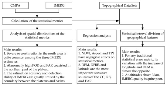
Figure 5.
The flowchart of the analysis of the traditional statistical error metrics.
4.2. Independent Error Components
For all independent error components, the values of the regression model are between 0.51 and 0.62. Hit bias has the highest values (>0.60), while the values of other error components are relatively low (>0.51), illustrating that the regression model is an appropriate approach to show the relationships between the errors and the topographic features. Figure 6 represents the weight distributions of the seven geographical features in the three independent error components, and the total errors for all kinds of IMERG estimates. The results suggest that the effect of NDVI, aspect and TPI on these errors is negligible due to the sum of the three weights being less than 8%. That mirrors similar results shown in Figure 2. Therefore, the remaining analysis in subsequent sections will focus on the effect of the other five geographical features (longitude, latitude, DFBE, DEM, and slope) on the errors.
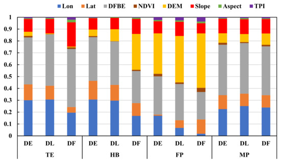
Figure 6.
Same as Figure 2 but based on independent error components.
The longitude and DFBE (weights > 0.3) are major sources of the high sensitivity-of-hit bias for IMERG-DE and DL, followed by latitude, DEM, and slope (weights < 0.15). However, for IMERG-DF, DEM replaced longitude and together with DFBE as the most significant contributors to the high sensitivity of hit bias (weights > 0.3). Besides, DEM and DFBE are also the leading causes of false precipitation for the three IMERG estimates, and the sum of the weights for the three estimates is around 0.7. For missed precipitation, the most significant contributor to the errors is DFBE (weight > 0.42), followed by longitude (weight > 0.23). In general, from IMERG-DE to DL, to DF, the weights of DEM in hit bias and false precipitation are continuously increasing, while the weights of longitude are decreasing. Finally, due to the combined influence of the three independent error components, the largest contributor to the total errors of the three IMERG estimates is DFBE, and the other two main error determinants are longitude and slope.
The spatial distributions of the total errors and their independent components are displayed in Figure 7. The three IMERG estimates are similar in spatial distribution of total errors and individual error components. One of the most obvious features is the total errors and hit bias of the three IMERG estimates all being positive in the basin area, but negative at the boundary between the plateau and basin. Moreover, the missed precipitation for the three IMERG products is evenly distributed over the entire region with small values. The false precipitation in the plateau region is much larger than that of other regions, and the false precipitation in the plateau region has a similar spatial distribution as that of the total errors.
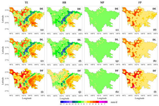
Figure 7.
Spatial distributions of mean errors components for the three IMERG estimates: columns from left to right are (a,e,i) total errors (TE), (b,f,j) hit bias (HB), (c,g,k) missed precipitation (MP), and (d,h,l) false precipitation (FP), respectively; rows from top down are IMERG-DE, IMERG-DL, and IMERG-DF, respectively. The error components are related by TE = HB + MP + FP, all in mm/d.
However, there are some differences in the spatial distribution of errors for the three IMERG estimates. Specifically, the NRT IMERG and IMERG-DF show the opposite capability of the hit bias in the plateau region, that is, the former underestimates precipitation while the latter overestimates it. Furthermore, the hit bias of the NRT IMERG reveals greater estimate errors than that of IMERG-DF at the boundary between the plateau and basin, but the errors of false precipitation from the former are smaller than those of the latter. The total errors are determined by the three independent error components, and thus the total errors of the IMERG-DF are positive scores in the entire region, while the total errors of the NRT IMERG show negative scores in large areas of the plateau (see Figure 7a,e,l).
The above analysis shows that the errors of IMERG-DL, and DF do not reduce greatly in comparison to those of IMERG-DE, which indicates that the bias correction scheme used in IMERG-DL does not suppress the three independent error components efficiently. However, we find that the total errors of IMERG-DF are the sum of the total error of NRT IMERG daily estimates and an additional positive bias, which causes the severe underestimation in the original estimates to be mitigated and the slight overestimation to be exacerbated. This additional positive bias mainly comes from the significantly increased hit bias and false precipitation, which may be caused by the calibration using the GPCC monthly observation during the generation of IMERG-DF.
As can be seen from Figure 8, the curves for IMERG-DE and DL almost completely overlap with any geographical features, indicating that the two estimates have the same variation in errors. Additionally, the total errors, hit bias, and false precipitation of IMERG-DF are always larger than those of IMERG-DE and DL, while the missed precipitation curves of the three IMERG estimates are all horizontal straight lines with amplitudes around 0. The above results show that geographical features have a large impact on hit bias and false precipitation, but hardly affect missed precipitation. Therefore, the following analysis will be focused on these two error components (i.e., HB and FP).
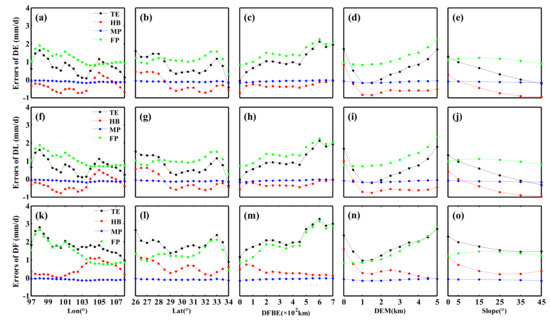
Figure 8.
The distribution of total errors and three independent components with five geographical features for the IMERG-DE, DL, and DF estimates. From left to right, five columns represent longitude (a,f,k), latitude (b,g,l), DFBE (c,h,m), DEM (d,i,n), and slope (e,j,o), respectively. From top to bottom, three rows represent errors of IMERG-DE (a–e), DL (f–j), and DF (k–o), respectively.
As longitude increases, false precipitation exhibits larger amplitudes and more severe fluctuations than hit bias in the region below 102°E, which being highly similar to the total errors. This indicates that longitude has a greater impact on false precipitation than hit bias, but this effect is positive. Meanwhile, false precipitation is the most important contributor to the total errors. However, in high longitude regions, false precipitation remains stable around 1.0 mm/d, but hit bias shows large fluctuations. That is to say, the increased longitude has no relationship with the performance of false precipitation, but seriously affected hit bias. Besides, although the magnitudes of the total errors in this region come from hit bias and false precipitation, their trends are almost entirely determined by hit bias.
With increasing latitude, hit bias and false precipitation show downward fluctuation and relatively stable change trends, respectively, until 31°N is reached. Above this latitude, both error components increase rapidly, with a peak at 33°N. Furthermore, after comparing the fluctuation amplitudes of the hit bias and false precipitation, we found that the sensitivity of hit bias is amplified at low latitudes, while the large fluctuation of false precipitation occurred at high latitudes. Finally, combined with the changing trend of the total errors, we can conclude that the fluctuation of the total errors at the low and high latitudes is mainly determined by hit bias and false precipitation, respectively.
As for DFBE, hit bias shows more obvious fluctuations than false precipitation within a small area of 100 km, and its trend is very similar to the total errors. Beyond 100 km, hit bias remains stable, while false precipitation shows the same upward trend as the total errors and peaks at 600 km. From the above analysis, it can be seen that for most areas of DFBE, the increase in DFBE presents a significant negative impact on false precipitation, but hardly affects hit bias.
Below 1.5 km, hit bias decreases rapidly with the increase in DEM, while false precipitation remains stable around 0.8 mm/d. Above this elevation, the former gradually stabilize, while the latter rapidly increases. This indicates that DEM at low altitude mainly affects hit bias, and the increase in DEM can effectively suppress hit bias. However, in the high elevation, the strong impact of DEM is evident for false precipitation compared to hit bias, and the increase in DEM has a significant negative effect on the control of error.
Regarding slope, both total errors and hit bias show a decreasing trend and the gap between them remains stable, while false precipitation is relatively constant with almost negligible variations. It can be concluded that the increase in slope has a strong negative influence to hit bias but has almost no relationship with false precipitation. The same is true for Figure 5, and the flowchart of this subsection is shown in Figure 9.
Figure 9.
The flowchart of the analysis of independent error components.
4.3. Systematic and Random Errors
The systematic and random errors of hit precipitation are separated based on the multiplicative model, and then the relationships between them and geographical features are analyzed by the regression method. For a given geographic feature, because systematic and random errors are complementary, the standard regression coefficients of systematic errors and random errors have equal absolute values but opposite signs, suggesting their weight distributions are the same. Therefore, only the results related to systematic errors are shown in Figure 10.
Figure 10.
Same as Figure 6 but based on systematic errors.
The results clearly show that longitude, latitude, DFBE, DEM, and slope have significant effects on the systematic and random errors of all IMERG estimates, and the weight values of aspect and TPI are almost negligible. For IMERG-DE, the first four geographical features have similar weight values, which are almost twice the weight values of the slope. Compared with IMERG-DE, the weight value of latitude in IMERG-DL decreases significantly (from 0.2 to 0.1). For IMERG-DF, DEM is the most critical error determinant, and its weight value is far ahead of that of other geographical features. At the same time, we also found that with the increasing complexity of error correction schemes from IMERG-DE to DL and then to DF, the role of DEM in error determination is becoming more and more important, while the influence of slope and latitude is declining.
Figure 11 shows the spatial distributions of systematic and random errors of the three IMERG estimates. Systematic errors of NRT IMERG exhibit large spatial variations in plateau and basin regions. Errors in the plateau are notably larger than those in the basin, and the peak appears in their border area. The systematic errors of IMERG-DF show better spatial homogeneity across the whole region and have smaller values. In contrast, because random errors are complementary to systematic errors, the areas with small systematic errors will have larger random errors. The comparison results of the three IMERG estimates indicate that the backward-morphing scheme and bias adjustment using a climatological gauge cannot effectively suppress the systematic errors of IMERG-DL in the plateau, which are greatly reduced in IMERG-DF calibrated by GPCC monthly observations. These conclusions suggest that NRT IMERG should focus more on the fast error correction algorithm to reduce systematic errors of IMERG estimates in complex terrain.
Figure 11.
Spatial distributions of systematic errors (the first row, a–c) and random errors (the second row, d–f) in percentage form for the three IMERG estimates. From left to right, three columns represent IMERG-DE (a,d), DL (b,e), and DF (c,f), respectively.
With the change in geographical features, the performance of the systematic errors of IMERG estimates is shown in Figure 12. Figure 12 shows that the systematic error variation curves of IMERG-DE and DL are highly consistent and have larger fluctuation amplitudes and overall amplitudes than IMERG-DF. More specifically, the systematic errors of NRT IMERG show an obvious growth trend with the increase in DFBE, DEM, and slope, but show a decreasing and increasing trend with the increase in longitude and latitude, respectively, which then reverse when a specific high longitude and latitude (105°E or 32°N) are reached. Regarding IMERG-DF, its systematic errors keep steady in most regions of all geographical features and only fluctuate greatly in the high-value regions of longitude, latitude, DFBE, or DEM. The above analysis shows that the systematic errors of NRT IMERG are mostly sensitive to the variations in these geographical features. However, this high sensitivity is greatly inhibited in IMERG-DF, but the sharp increase in systematic errors in areas far from the basin and at high altitude cannot be ignored. The same as in Figure 5, the flowchart of this subsection is shown in Figure 13.
Figure 12.
Relationships between systematic errors and five geographical features for three IMERG estimates. (a–e) represent longitude, latitude, DFBE, DEM, and Slope, respectively.
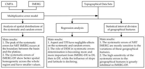
Figure 13.
The flowchart of the analysis of the systematic errors.
5. Discussion
The characteristic of the elevation in this study (high in the west and low in the east, see Figure 1a) suggests that the longitude is correlated with changes in the elevation. The first, third, and fourth rows of Figure 4 clearly show that for any traditional statistical error metric, its variation with the increase in longitude and DEM is almost the opposite. In addition, similar to the elevation, the increase in DFBE has a negative influence on the quality of IMERG estimates. Meanwhile, similar variations are also found in the correlation analysis of independent error components, systematic errors, and random errors with geographical features (see Figure 8 and Figure 12). The above analysis indicates that longitude and DFBE do not have a direct impact on the errors, but indirectly affect the precipitation errors through the changing DEM. Therefore, we can reasonably believe that the influence patterns of longitude and DFBE are a reflection of the change in DEM.
Most of the precipitation error metrics exhibit high sensitivity to DEM and latitude changes, especially in regions with elevations greater than 1 km or latitudes higher than 30°N. With the increase in DEM and latitude, the ground temperature shows a clear downward trend. Therefore, DEM and latitude could partly represent the temperature, then influence the atmospheric circulation and precipitation phase, and ultimately affect the quality of satellite precipitation estimates. In general, the quality of IMERG estimates would decrease with the increasing DEM and latitude. The most likely reasons are: (1) IR brightness temperature, which is an important data source for the generation of IMERG estimates, is more effective in identifying no-rain instances in areas with high ground temperatures; however, this effectiveness is reduced in cold regions [24]. This indicates that the quality of IMERG estimates would decrease with the temperature drops; (2) DEM will distort the interpolation results because the applied algorithm often assumes that the surface is flat [50]; (3) high DEM has a major influence on the structure of the precipitation field, thereby promoting the generation of convective precipitation with a scale smaller than the spatial resolution of GPM, which may seriously enlarge the error of satellite precipitation estimates [51]; (4) the snow/ice-covered land surfaces, caused by low ground temperature, can also cause large uncertainty in precipitation measurements, especially in high-DEM and high-latitude regions; (5) thick fog often occurs at high DEM and high-latitude areas with lower ground temperatures. Therefore, the sizes of fog or cloud droplets that are increased by higher concentrations of aerosols in these regions may intercept the capability of precipitation estimation by the IMERG estimations, which leads to high false precipitation [52]; and (6) high DEM could become a hindrance to the vertical and horizontal moist wind from the eastern part of the study area. Besides, the low temperature caused by high elevation also has an obvious cooling influence on convection currents and the moist winds from the warm region [53].
Additionally, we note that the obvious shift in the curves of almost all the error metrics occurs around 33°N. This phenomenon should be attributed to the sparse networks of ground observations in this area. We treated the gauge reference data as error-free when evaluating the quality of the IMERG estimates, which is not true (even though a necessary bias adjustment of gauge-based observations has been applied to correct the undercatch bias). Therefore, the ground reference data at the high end of latitude and DEM is under quality control [36], which may weaken the robustness and reliability of our results.
6. Conclusions
Many previous precipitation assessment studies have expounded that satellite precipitation performs worse in complex terrain areas. However, the relationships between these precipitation errors and geographical features have not been systematically investigated and compared. In this study, we have characterized and compared the spatial distributions of summer precipitation errors for the three IMERG estimates over Sichuan, which has a unique complex terrain in southwestern China. Afterward, the comprehensive analysis was carried out on the inner connections between spatial variations in errors and geographical features (e.g., longitude, latitude, DFBE, DEM, Slope, etc.) with the continuous and statistical metrics, independent error components, systematic and random errors, etc. The main conclusions are summarized as follows:
Both aspect and TPI have significantly smaller weights than other geographical features for all error metrics, and their influences can be ignored. DEM is the leading factor to determine the changes in CC and false precipitation. The quality of IMERG estimates decreases (CC < 0.5, RB > 100%, FAR > 0.4) and the false precipitation increases rapidly with the increase in DEM on elevations above 2.5 km. However, in the lower regions (DEM < 1.5 km), the increased DEM plays a positive role in reducing the hit bias. It mainly suppresses the random errors of hit bias, but also amplifies the systematic errors of hit bias.
DFBE shows the most prominent effect on RB, POD, and FAR, and it is also an important factor leading to the high sensitivity of CC. Overall, the increase in DFBE has a negative relationship with the variations in the statistical error metrics, except for POD. In addition, the high sensitivity of hit bias is mainly reflected in the low end (DFBE < 100 km), while false precipitation shows an increasing trend throughout the entire range of DFBE. Similar to DEM, the systematic errors of hit bias continue to grow linearly with DFBE.
For latitude, the influence on RB, POD, and FAR is second only to DFBE. Specifically, in the low and high regions (<27.5°N and >33°N), RB and FAR are significantly improved with increasing latitude. However, in the intermediate region (30.5°N–33°N), all statistical metrics show a sharp deterioration. Furthermore, although latitude has a relatively small weight among the three independent error components, its contribution is still non-negligible. At the low end (<31°N), hit bias shows a downward trend, while false precipitation remains stable, and this situation is in contrast to that of the other regions (in other regions, hit bias is relatively stable while false precipitation experiences larger fluctuations). Additionally, the changes and fluctuations of the systematic errors from IMERG-DE and DL are much larger than those of IMERG-DF, indicating that the increasing latitude has a significantly greater negative impact on the former than that of the latter.
POD and FAR are also sensitive to changes in longitude, but the sensitivity is slightly weaker than that of latitude. But in general, for any traditional statistical error metric, its variation with the increase in longitude and DEM is almost the opposite. This suggests that longitude does not have a direct impact on the errors, but is often related to changes in other variables (e.g., DEM and ground temperature) that are directly related to errors. Compared to longitude, latitude, DFBE, and DEM, the slope has the least influence on all error metrics. The increasing slope slightly reduces the overestimation of IMERG estimates and also weakens the CC. Furthermore, slope shows a strong negative relationship with hit bias, but is not highly correlated to false precipitation. Besides, the increasing slope amplifies the systematic errors of all three estimates, where IMERG-DE and DL show higher sensitivity than that of IMERG-DF.
Both POD and MP show weaker fluctuations and better performances than other error metrics with the change in geographical features, which means that the excellent detection capability for hit precipitation and the superior suppression capability for miss precipitation of IMERG estimates are almost independent of the change in geographical features.
By analyzing the relationships between the error metrics in the three IMERG estimates and various geographical features, the findings of this work provide valuable reference and feedback for IMERG producers to infer the sources of precipitation estimation errors in complex topographical areas.
Author Contributions
Conceptualization, R.L. and S.T.; methodology, S.T.; funding acquisition, S.T.; resources, Z.S.; project administration, J.H.; visualization, W.S.; data curation, X.L.; software, R.L. and S.T.; writing—original draft, R.L.; writing—review and editing, S.T. All authors have read and agreed to the published version of the manuscript.
Funding
This work was supported by the National Key R&D Program of China (Grant No. 2021YFC3090203) and the Natural Science Foundation of Sichuan Province (Grant No. 2022NSFSC0209 and Grant No. 2022NSFSC0214).
Data Availability Statement
Not applicable.
Acknowledgments
We are grateful to the scientists in the National meteorological information center (NMIC) and National Aeronautics and Space Administration (NASA) for providing satellite precipitation data used in this paper. Special thanks to the National Meteorological Information Center (NMIC) and China Meteorological Administration (CMA) for providing the reference dataset (CMPA). We also thank the Geospatial Data Cloud site, Computer Network Information Center, Chinese Academy of Sciences for providing the topographical datasets. In addition, we wish to express our gratitude to the editor and the anonymous reviewers for their professional and constructive comments and suggestions, which were very helpful in providing for the further quality improvement of this manuscript.
Conflicts of Interest
The authors declare that they have no conflict of interest.
References
- Ma, S.; Zhou, T. Observed trends in the timing of wet and dry season in China and the associated changes in frequency and duration of daily precipitation. Int. J. Climatol. 2015, 35, 4631–4641. [Google Scholar] [CrossRef]
- Sadeghi, M.; Asanjan, A.A.; Faridzad, M.; Nguyen, P.; Hsu, K.; Sorooshian, S.; Braithwaite, D. PERSIANN-CNN: Precipitation Estimation from Remotely Sensed Information Using Artificial Neural Networks–Convolutional Neural Networks. J. Hydrometeorol. 2019, 20, 2273–2289. [Google Scholar] [CrossRef]
- Hou, A.Y.; Kakar, R.K.; Neeck, S.P.; Azarbarzin, A.A.; Kummerow, C.D.; Kojima, M.; Oki, R.; Nakamura, K.; Iguchi, T. The Global Precipitation Measurement Mission. Bull. Am. Meteorol. Soc. 2014, 95, 701–722. [Google Scholar] [CrossRef]
- Li, N.; Wang, Z.; Sun, K.; Chu, Z.; Leng, L.; Lv, X. A Quality Control Method of Ground-Based Weather Radar Data Based on Statistics. IEEE Trans. Geosci. Remote Sens. 2017, 56, 2211–2219. [Google Scholar] [CrossRef]
- Tang, G.; Ma, Y.; Long, D.; Zhong, L.; Hong, Y. Evaluation of GPM Day-1 IMERG and TMPA Version-7 legacy products over Mainland China at multiple spatiotemporal scales. J. Hydrol. 2016, 533, 152–167. [Google Scholar] [CrossRef]
- Lu, X.; Wei, M.; Tang, G.; Zhang, Y. Evaluation and correction of the TRMM 3B43V7 and GPM 3IMERGM satellite precipitation products by use of ground-based data over Xinjiang, China. Environ. Earth Sci. 2018, 77, 209. [Google Scholar] [CrossRef]
- Arkin, P.A.; Xie, P. The global precipitation climatology project: First algorithm intercomparison project. Bull. Am. Meteorol. Soc. 1994, 75, 401–420. [Google Scholar] [CrossRef]
- Hsu, K.-l.; Gao, X.; Sorooshian, S.; Gupta, H.V. Precipitation estimation from remotely sensed information using artificial neural networks. J. Appl. Meteorol. Climatol. 1997, 36, 1176–1190. [Google Scholar] [CrossRef]
- Joyce, R.; Janowiak, J.E.; Arkin, P.A.; Xie, P. CMORPH: A Method that Produces Global Precipitation Estimates from Passive Microwave and Infrared Data at High Spatial and Temporal Resolution. J. Hydrometeorol. 2004, 5, 487–503. [Google Scholar] [CrossRef]
- Huffman, G.J.; Bolvin, D.T.; Nelkin, E.J.; Wolff, D.B.; Adler, R.F.; Gu, G.; Hong, Y.; Bowman, K.P.; Stocker, E.F. The TRMM multisatellite precipitation analysis (TMPA): Quasi-global, multiyear, combined-sensor precipitation estimates at fine scales. J. Hydrometeorol. 2007, 8, 38–55. [Google Scholar] [CrossRef]
- Kubota, T.; Shige, S.; Hashizume, H.; Aonashi, K.; Takahashi, N.; Seto, S.; Hirose, M.; Takayabu, Y.N.; Ushio, T.; Nakagawa, K. Global precipitation map using satellite-borne microwave radiometers by the GSMaP project: Production and validation. IEEE Trans. Geosci. Remote Sens. 2007, 45, 2259–2275. [Google Scholar] [CrossRef]
- Huffman, G.J.; Bolvin, D.T.; Braithwaite, D.; Hsu, K.; Joyce, R.; Xie, P.; Yoo, S.-H. NASA global precipitation measurement (GPM) integrated multi-satellite retrievals for GPM (IMERG). Algorithm Theor. Basis Doc. 2015, 4, 26. [Google Scholar]
- Kummerow, C.D.; Barnes, W.L.; Kozu, T.; Shiue, J.; Simpson, J. The Tropical Rainfall Measuring Mission (TRMM) Sensor Package. J. Atmos. Ocean. Technol. 1998, 15, 809–817. [Google Scholar] [CrossRef]
- Panegrossi, G.; Rysman, J.-F.; Casella, D.; Marra, A.C.; Sanò, P.; Kulie, M.S. CloudSat-based assessment of GPM Microwave Imager snowfall observation capabilities. Remote Sens. 2017, 9, 1263. [Google Scholar] [CrossRef]
- Tong, K.; Su, F.; Yang, D.; Hao, Z. Evaluation of satellite precipitation retrievals and their potential utilities in hydrologic modeling over the Tibetan Plateau. J. Hydrol. 2014, 519, 423–437. [Google Scholar] [CrossRef]
- Hosseini-Moghari, S.-M.; Tang, Q. Validation of GPM IMERG V05 and V06 precipitation products over Iran. J. Hydrometeorol. 2020, 21, 1011–1037. [Google Scholar] [CrossRef]
- Zhou, C.; Gao, W.; Hu, J.; Du, L.; Du, L. Capability of imerg v6 early, late, and final precipitation products for monitoring extreme precipitation events. Remote Sens. 2021, 13, 689. [Google Scholar] [CrossRef]
- Chen, F.; Li, X. Evaluation of IMERG and TRMM 3B43 monthly precipitation products over mainland China. Remote Sens. 2016, 8, 472. [Google Scholar] [CrossRef]
- Guo, H.; Bao, A.; Ndayisaba, F.; Liu, T.; Kurban, A.; De Maeyer, P. Systematical Evaluation of Satellite Precipitation Estimates Over Central Asia Using an Improved Error-Component Procedure. J. Geophys. Res. Atmos. 2017, 122, 10906–10927. [Google Scholar] [CrossRef]
- Zhang, C.; Chen, X.; Shao, H.; Chen, S.; Liu, T.; Chen, C.; Ding, Q.; Du, H. Evaluation and Intercomparison of High-Resolution Satellite Precipitation Estimates—GPM, TRMM, and CMORPH in the Tianshan Mountain Area. Remote Sens. 2018, 10, 1543. [Google Scholar] [CrossRef]
- Tang, S.; Li, R.; He, J.; Wang, H.; Fan, X.; Yao, S. Comparative Evaluation of the GPM IMERG Early, Late, and Final Hourly Precipitation Products Using the CMPA Data over Sichuan Basin of China. Water 2020, 12, 554. [Google Scholar] [CrossRef]
- Yong, B.; Chen, B.; Gourley, J.J.; Ren, L.; Hong, Y.; Chen, X.; Wang, W.; Chen, S.; Gong, L. Intercomparison of the Version-6 and Version-7 TMPA precipitation products over high and low latitudes basins with independent gauge networks: Is the newer version better in both real-time and post-real-time analysis for water resources and hydrologic extremes? J. Hydrol. 2014, 508, 77–87. [Google Scholar] [CrossRef]
- Iguchi, T.; Kozu, T.; Kwiatkowski, J.; Meneghini, R.; Awaka, J.; Okamoto, K.i. Uncertainties in the rain profiling algorithm for the TRMM precipitation radar. J. Meteorol. Soc. Japan. Ser. II 2009, 87, 1–30. [Google Scholar] [CrossRef]
- Ombadi, M.; Nguyen, P.; Sorooshian, S.; Hsu, K.-l. How much information on precipitation is contained in satellite infrared imagery? Atmos. Res. 2021, 256, 105578. [Google Scholar] [CrossRef]
- Liu, B.; Wan, W.; Xie, H.; Li, H.; Zhu, S.; Zhang, G.; Wen, L.; Hong, Y. A long-term dataset of lake surface water temperature over the Tibetan Plateau derived from AVHRR 1981–2015. Sci. Data 2019, 6, 48. [Google Scholar] [CrossRef] [PubMed]
- Ma, Z.; Shi, Z.; Zhou, Y.; Xu, J.; Yu, W.; Yang, Y. A spatial data mining algorithm for downscaling TMPA 3B43 V7 data over the Qinghai–Tibet Plateau with the effects of systematic anomalies removed. Remote Sens. Environ. 2017, 200, 378–395. [Google Scholar] [CrossRef]
- Zhu, S.; Wan, W.; Xie, H.; Liu, B.; Li, H.; Hong, Y. An efficient and effective approach for georeferencing AVHRR and GaoFen-1 imageries using inland water bodies. IEEE J. Sel. Top. Appl. Earth Obs. Remote Sens. 2018, 11, 2491–2500. [Google Scholar] [CrossRef]
- Wang, X.; Ding, Y.; Zhao, C.; Wang, J. Similarities and improvements of GPM IMERG upon TRMM 3B42 precipitation product under complex topographic and climatic conditions over Hexi region, Northeastern Tibetan Plateau. Atmos. Res. 2019, 218, 347–363. [Google Scholar] [CrossRef]
- Yang, M.; Liu, G.; Chen, T.; Chen, Y.; Xia, C. Evaluation of GPM IMERG precipitation products with the point rain gauge records over Sichuan, China. Atmos. Res. 2020, 246, 105101. [Google Scholar] [CrossRef]
- Zhu, S.; Shen, Y.; Ma, Z. A New Perspective for Charactering the Spatio-temporal Patterns of the Error in GPM IMERG Over Mainland China. Earth Space Sci. 2021, 8, 16. [Google Scholar] [CrossRef]
- Dan, C.; Changyan, Z.; Guangming, X.; Mengyu, D. Characteristics of Climate Change of Summer Rainstorm in Sichuan Basin in the Last 53 Years. Plateau Meteorol. 2018, 37, 197–206. [Google Scholar]
- Yu, L.; Chao, C.; Jia, L.; LI, X.-l.; Rong, Y. Characteristics and causes of regional extreme precipitation events in summer over Sichuan Basin. J. Southwest Univ. 2019, 41, 128–138. [Google Scholar]
- Zhou, Q.; Kang, L.; Jiang, X.; Liu, Y. Relationship between heavy rainfall and altitude in mountainous areas of Sichuan basin. Meteorol. Monogr. 2019, 45, 811–819. [Google Scholar] [CrossRef]
- Shen, P.F.; Zhang, Y.C. Numerical Simulation of Diurnal Variation of Summer Precipitation in Sichuan Basin. Plateau Meteorol. 2011, 30, 860–868. [Google Scholar]
- Sungmin, O.; Foelsche, U.; Kirchengast, G.; Fuchsberger, J.; Tan, J.; Petersen, W.A. Evaluation of GPM IMERG Early, Late, and Final rainfall estimates using WegenerNet gauge data in southeastern Austria. Hydrol. Earth Syst. Sci. 2017, 21, 6559–6572. [Google Scholar] [CrossRef]
- Shen, Y.; Zhao, P.; Pan, Y.; Yu, J. A high spatiotemporal gauge-satellite merged precipitation analysis over China. J. Geophys. Res. 2014, 119, 3063–3075. [Google Scholar] [CrossRef]
- Su, J.; Lü, H.; Crow, W.T.; Zhu, Y.; Cui, Y. The effect of spatiotemporal resolution degradation on the accuracy of IMERG products over the Huai River basin. J. Hydrometeorol. 2020, 21, 1073–1088. [Google Scholar] [CrossRef]
- Su, J.; Lu, H.; Zhu, Y.; Wang, X.; Wei, G. Component Analysis of Errors in Four GPM-Based Precipitation Estimations over Mainland China. Remote Sens. 2018, 10, 1420. [Google Scholar] [CrossRef]
- Tang, G. Characterization of the Systematic and Random Errors in Satellite Precipitation Using the Multiplicative Error Model. IEEE Trans. Geosci. Remote Sens. 2020, 59, 5407–5416. [Google Scholar] [CrossRef]
- Ma, Y.; Zhang, Y.; Yang, D.; Farhan, S.B. Precipitation bias variability versus various gauges under different climatic conditions over the Third Pole Environment (TPE) region. Int. J. Climatol. 2015, 35, 1201–1211. [Google Scholar] [CrossRef]
- Jarvis, A.; Reuter, H.I.; Nelson, A.; Guevara, E. Hole-Filled SRTM for the Globe Version 4. 2008. Available online: Http://srtm.csi.cgiar.org (accessed on 15 January 2022).
- Skidmore, A.K. A comparison of techniques for calculating gradient and aspect from a gridded digital elevation model. Int. J. Geogr. Inf. Syst. 1989, 3, 323–334. [Google Scholar] [CrossRef]
- Weiss, A. Topographic position and landforms analysis. In Proceedings of the Poster Presentation, ESRI User Conference, San Diego, CA, USA, 9–13 July 2001. [Google Scholar]
- Makarieva, A.M.; Gorshkov, V.G.; Li, B.-L. Precipitation on land versus distance from the ocean: Evidence for a forest pump of atmospheric moisture. Ecol. Complex. 2009, 6, 302–307. [Google Scholar] [CrossRef]
- Tian, Y.; Peters-Lidard, C.D.; Eylander, J.B.; Joyce, R.J.; Huffman, G.J.; Adler, R.F.; Hsu, K.l.; Turk, F.J.; Garcia, M.; Zeng, J. Component analysis of errors in satellite-based precipitation estimates. J. Geophys. Res. Atmos. 2009, 114. [Google Scholar] [CrossRef]
- Tian, Y.; Huffman, G.J.; Adler, R.F.; Tang, L.; Sapiano, M.; Maggioni, V.; Wu, H. Modeling errors in daily precipitation measurements: Additive or multiplicative? Geophys. Res. Lett. 2013, 40, 2060–2065. [Google Scholar] [CrossRef]
- Tang, S.; Li, R.; He, J. Modeling and Evaluating Systematic and Random Errors in Multiscale GPM IMERG Summer Precipitation Estimates Over the Sichuan Basin. IEEE J. Sel. Top. Appl. Earth Obs. Remote Sens. 2021, 14, 4709–4719. [Google Scholar] [CrossRef]
- Willmott, C.J. On the validation of models. Phys. Geogr. 1981, 2, 184–194. [Google Scholar] [CrossRef]
- Aghakouchak, A.; Mehran, A.; Norouzi, H.; Behrangi, A. Systematic and random error components in satellite precipitation data sets. Geophys. Res. Lett. 2012, 39. [Google Scholar] [CrossRef]
- Haiden, T.; Pistotnik, G. Intensity-dependent parameterization of elevation effects in precipitation analysis. Adv. Geosci. 2009, 20, 33–38. [Google Scholar] [CrossRef]
- Sharifi, E.; Steinacker, R.; Saghafian, B. Assessment of GPM-IMERG and Other Precipitation Products against Gauge Data under Different Topographic and Climatic Conditions in Iran: Preliminary Results. Remote Sens. 2016, 8, 135. [Google Scholar] [CrossRef]
- Dipu, S.; Prabha, T.V.; Pandithurai, G.; Dudhia, J.; Pfister, G.; Rajesh, K.; Goswami, B.N. Impact of elevated aerosol layer on the cloud macrophysical properties prior to monsoon onset. Atmos. Environ. 2013, 70, 454–467. [Google Scholar] [CrossRef]
- Basist, A.; Bell, G.D.; Meentemeyer, V. Statistical relationships between topography and precipitation patterns. J. Clim. 1994, 7, 1305–1315. [Google Scholar] [CrossRef]
Publisher’s Note: MDPI stays neutral with regard to jurisdictional claims in published maps and institutional affiliations. |
© 2022 by the authors. Licensee MDPI, Basel, Switzerland. This article is an open access article distributed under the terms and conditions of the Creative Commons Attribution (CC BY) license (https://creativecommons.org/licenses/by/4.0/).