1. Introduction
In recent years, automation is becoming more and more critical in the automotive industry. Simple parking assistance systems are becoming standard technology for modern cars, while fully autonomous driving systems appear to be just a few years ahead of us. All these technologies are supported by a variety of different sensors such as optical cameras, LiDAR, and radars [
1].
In the literature, several imaging algorithms are detailed using one or the combination of more sensors. In [
2], for example, a LiDAR is used to obtain an accurate map of the surrounding environment in combination with a refined scanning algorithms allowing for a much lower scanning time. In [
3], instead, a super-resolution algorithm is applied to improve the accuracy of the urban mapping.
This paper, however, treats the problem of imaging using radars. Such sensors have specific peculiarities that make them attractive to the automotive industry. First of all, the radar is an active sensor; therefore, the instrument provides illumination. Being able to control the illumination of the scene allows for flexibility in terms of spatial resolution (that is adjustable by changing the bandwidth of the transmitted signal) and permits day and night imaging of the environment. Radars operating at microwave are also not particularly sensitive to fog, rain, and snow, which are three typical environmental scenarios that create troubles for LiDAR and cameras.
The drawback of conventional automotive radar imaging is the poor angular resolution. Such systems typically employ a Multiple-Input Multiple-Output (MIMO) architecture to generate a virtual array that achieves some angular resolution. However, such resolution is bounded by the length of the array and could be in the order of tens of degrees [
4].
Recently, a lot of effort has been carried out in the field of automotive-based Synthetic Aperture Radar (SAR) imaging. This technique, known for decades in space-borne and air-borne radar imaging, has been rarely applied in the automotive industry. SAR imaging exploits several radar pulses transmitted by a moving platform (in this case, a vehicle) to synthesize a very long array leading to a much finer resolution than conventional radar imaging [
5].
The first experiments for what concerns automotive SAR imaging are the ones carried out in [
6] using a very high frequency and wide bandwidth radar mounted on a vehicle. This work shows the capabilities of SAR systems but requires costly hardware and it is not suited for real-time applications due to large computational burden.
Recent works also demonstrated the capabilities of car-based SAR imaging to map the urban environment. In [
7,
8], the authors carried out several laboratory tests using a forward-looking SAR and by exploiting compressive sensing. Other works include the one in [
9] where a TDM (Time Division Multiplexing) MIMO radar has been used to form SAR images of the surroundings. The well-known focusing algorithm (the Range–Doppler algorithm with secondary migration correction) was also tested in the automotive scenario showing good performances, at least for linear trajectories [
10]. The state of the art is currently represented by [
11,
12,
13] where real data are used, which were acquired in an urban scenario and exploiting non-linear trajectories of the car.
In [
14], the necessity of an autofocus algorithm has been made clear: fine image resolution and short wavelengths demand high accuracy in the knowledge of the vehicle’s trajectory. The requested accuracy can be as low as 1–2 cm/s. Such precision cannot be reached by standard automotive grade Navigation Units (NU); thus, a proper autofocusing algorithm is mandatory. The approach proposed in [
14] exploits a set of low-resolution images focused thanks to the presence of a virtual array to recover a residual motion velocity, leading to a well-focused and well-localized image.
The contribution of this paper consists of describing and comparing three algorithms that can be used to combine low-resolution MIMO images to obtain the final focused SAR image. The analytical foundation of each algorithm is derived, and their limitations are also explained in details.
In
Section 2, the geometry of the system is explained and the processing steps that lead to a set of coregistered MIMO images are detailed.
In
Section 3.1, the first algorithm, the Fast-Factorized Back-Projection (FFBP) is described, while in
Section 3.2, the same thing is completed on the second algorithm, which is called 3D2D. The origin of this name will be explained in the corresponding section. In the same section, we propose a variation of the algorithm called Quick & Dirty (Q&D). It is a version of 3D2D which avoids the compensation of range migration and phase curvature. Its strong limitations compared to the two previously listed algorithms will be detailed in the same section.
Section 4 provides results with simulated data. This section compares the two algorithms using different interpolation kernels and different aperture lengths by assessing the quality of the Impulse Response Function (IRF) using appropriate metrics such as the normalized peak value and the Integrated Side Lobe Ration (ISLR). In
Section 5, a rough estimate of the number of operations required by the algorithms to form the final SAR image is provided to the reader.
Section 6 provides the results of the open road campaign carried out using a 77 GHz MIMO radar in a forward-looking configuration. Finally, in
Section 7, the conclusions are drawn.
2. Acquisition Geometry and MIMO Image Formation
2.1. Geometry and Signal Model
The system is composed of a vehicle (the moving platform) and a MIMO radar. The radar transmits an impulse with a specific bandwidth, leading to a slant range resolution of [
15]:
where
is the slant range resolution,
c is the speed of light and
B is the transmitted bandwidth.
Thanks to the presence of multiple channels, the radar generates the so-called
virtual array obtaining in this way angular resolution. The angular resolution depends on the wavelength, and it is inversely proportional to the length of the virtual array:
where
is the angular resolution,
is the central wavelength of the radar (
being the central frequency),
is the number of channels (Virtual Antenna Phase Center, VAPC),
d is the spacing between each virtual antenna,
is the azimuth angle and
is the radar installation angle.
In
Figure 1a, the geometry of the forward-looking system is depicted (
deg). For the sake of simplicity, the 2D scenario is represented. The antenna elements are the red dots displaced in the direction orthogonal to the motion.
While the car is moving, the MIMO radar transmits and receives the backscattered echos. We remark that for each time instant
, a number of signals equal to
are received. In
Figure 1b, a car travels at velocity
v in a straight trajectory and acquires every PRI seconds (Pulse Repetition Interval) a set of
signals.
The raw data are compressed [
16], leading to the range of compressed data
where
r is the range,
i is the index of the sensor (
), and
is the sampled slow-time variable. By neglecting the bistatic nature of the MIMO array, we can write the model of the range compressed data for a point target located at polar coordinates
:
where sinc is the cardinal sine function, and
is the one-way distance from the
VAPC to the target at the time instant
. Notice that in Equation (
3), we have also neglected an amplitude factor due to the spread loss and the Radar Cross-Section (RCS) of the target.
2.2. MIMO Image Formation
The simultaneous acquisitions can be used to focus a low-resolution image by a simple back-projection. In order to achieve high performances, it is convenient to avoid the back-projection on a Cartesian grid: the unnecessary high sampling of the signal leads to an unsustainable computational burden for real-time applications.
A significant improvement in performances can be achieved by back-projecting the signal on a polar grid [
17]. In this case, a fixed polar grid is defined in space as in
Figure 2 where each pixel has a range (
r) and angular position (
) defined with respect to the origin of the grid.
The low-resolution images can be formed now by a simple back-projection:
where
is the low-resolution radar image at coordinates
r and
, acquired at slow-time
, and
is the range compressed signal of the
channel evaluated at the range
. Notice that this range depends on the positions of the considered pixel (
r,
), on the position of the
virtual element at the slow-time
.
The focused image
is a pass-band image in the wavenumber domain with the before-mentioned resolutions (Equations (
1) and (
2)).
The important detail is that by back-projecting the range compressed data on a
fixed polar grid, each low-resolution image is already coregistered, the range migration has been compensated, and thus so has the phase curvature. We remark also that the back-projection is able to cope with any non-linear trajectory of the moving vehicle [
18].
The next step in the processing chain that will make it possible to obtain the well-focused high-resolution SAR image is the autofocus. Its objective is to estimate the trajectory residue (the one not estimated by the vehicle’s navigation unit). In the literature, there are several autofocusing techniques [
14,
19,
20,
21]. We remark, however, that each autofocus algorithm is based on a first detection of stable targets from low-resolution images. In this case, the low-resolution images are the
MIMO images themselves.
This is also the reason why in this article, we do not deal with frequency domain focusing algorithms: we need to have low-resolution images in order to estimate the residual motion. Once we have them, we look for ways to combine them in the most efficient way.
After the residual motion estimation and compensation, the final SAR image can be formed. We identified three possible techniques: namely, the Fast Factorized Back-Projection (FFBP), 3D2D, and a derivation of the latter called Quick&Dirty (Q&D) [
22]. In the following sections, the three methods are explained, their limitations and pitfalls are detailed, and they are compared in terms of performances.
3. SAR Imaging: Proposed Methods
The SAR processing foresees the coherent summation of each low-resolution image to obtain an SAR image at fine resolution:
Before the summation can happen, each low-res image must be demodulated, interpolated on a finer grid to accommodate for the expansion of the bandwidth induced by the coherent summation, and re-modulated.
In the following sections, we describe the two algorithms in detail, providing also a mathematical interpretation. The assumptions behind each algorithm are detailed, and the limits of each are indicated.
3.1. FFBP Scheme
The FFBP algorithm [
17] starts from the set of
low-res images discussed in
Section 2 and proceeds by interpolating sub-images in the angular domain to fine resolution before implementing the summation in Equation (
5). The block diagram of the processing is depicted in
Figure 3, and all the steps are here described:
- 1.
The images are divided into sub-groups composed each by images. This leads to the generation of sub-groups. Notice that each sub-group corresponds to a sub-aperture (i.e., to a portion of the total SAR aperture).
- 2.
Each of the
images is demodulated to bring them in base-band in the spatial frequency domain, avoiding in this way aliasing. This operation can be performed rigorously:
where
is the distance from the center of the virtual array to the pixel at coordinates (
r,
) at time
.
- 3.
Each image is now interpolated on a finer angular grid. The sampling of such a fine grid is computed by taking into account the current sub-aperture length (i.e., the PRI and the velocity of the vehicle). The interpolation is necessary to handle correctly the expansion of the bandwidth that will be generated in the following step.
where
represents the 1D interpolation in the angular direction on a finer grid.
- 4.
Every image is now modulated in order to bring them back into bandpass. The operation can be completed again rigorously as:
- 5.
All the images belonging to a sub-aperture are now coherently summed together, leading to a stack of
L images with higher resolution with respect to the original low-resolution stack.
where
stands for mid-resolution, meaning that the whole synthetic aperture has not been exploited yet.
l is the index of the sub-aperture (
), and the summation for the
sub-aperture is performed over all the images within that sub-aperture time
.
- 6.
All the steps described up to now are repeated with the only difference that we do not start anymore by the MIMO images but from the L mid-resolution SAR images, and the distances used for modulation and demodulation are computed from the center of the sub-aperture to each pixel and no more from the center of the virtual array.
The critical step of this procedure is the interpolation in (
7). We remark that while the car travels, the grid in
Figure 2 is fixed in space and defined only once for the entire synthetic aperture. The consequence is that the grid is strictly polar just for the low-resolution image having the array center co-located with the origin of the grid. As an example, we can take
Figure 2: in this case, just the last low-res image is back-projected on a grid that is truly polar. The previous three samples depicted in light red are back-projected on the same grid that is, however, not polar for them.
The result is an expansion of the bandwidth of the signal in the angular direction
that in turn leads to a possible error during interpolation in (
7). In the following, a theoretical treatment of this bandwidth expansion is proposed.
3.1.1. Limits and Drawbacks
Let us suppose to have a generic sensor placed in the origin of a Cartesian reference frame and a generic roto-translated polar grid as shown in
Figure 4.
By definition, the wavenumbers in the polar reference frame are defined as the partial derivatives of the distance in the range and angular direction. For a monocromatic wave, this leads to:
where
and
are the Cartesian coordinates of the polar grid origin,
is the rotation of the polar grid with respect to the Cartesian grid, and
r and
are the range and angular coordinates of the pixel in the polar grid.
Notice that, as expected, if the polar grid has the origin in the antenna phase center (, thus ), the wavenumber in the range direction is , while in the angular direction, it is zero. These considerations are easily extended for a wideband signal and for a virtual array composed of more than one antenna.
It is straightforward to see that a roto-translation of the polar back-projection grid will correspond to a bandwidth expansion of the signal in the angular direction, since
in Equation (
12) is no more zero. The angular sampling of the polar BP grid, however, is not designed to handle this bandwidth expansion; thus, aliasing occurs.
We deem that the solution to this problem is to wisely choose the polar BP grid. In particular, it is better to chose a grid that is as close to be polar as possible for all the antenna phase centers. One way to do so is to fix the origin of the grid at the center of the aperture. The quality of the image will also depend on the interpolation kernel used. Some tests have been carried out, and the results will be shown in
Section 4.
3.2. 3D2D Scheme
In this section, the 3D2D algorithm is detailed, and its limitations are explained. A block diagram of the algorithm is depicted in
Figure 5.
The algorithm starts again, as the FFBP, from the set of
low-resolution images discussed in
Section 2 and proceeds as follows:
- 1.
Each low-res image is demodulated into baseband using a linear law of distances. We use the linear approximation due to the fact that later on, a Fourier transform will be used, and the FT consists of applying a linear phase to the data and integrating it.
where we use the ≈ and not the = sign just to remember that the data are placed into baseband with an approximated law of distances given by:
In Equation (
14), the parameter
represents the distance from the center of the aperture to the pixel in
,
is the slow-time of the center of the aperture, and
is the radial velocity of the car with respect to a fixed target in
. This velocity is calculated exploiting the nominal trajectory provided by the NU, and it is calculated at the center of the aperture.
Notice that this is just a linear approximation of the true hyperbolic range equation; the linearity assumption holds for short aperture and/or far-range targets. An analysis of the validity of this assumption will be provided to the reader in
Section 3.2.2.
- 2.
The Fourier transform (FT) in the slow-time dimension of the baseband data is taken:
where
is the radial velocity and
is the Fourier transform in the slow-time direction. This leads to a dataset in the range, angle, and Doppler frequency domain that can be easily converted in range, angle, radial velocity. The output is the 3D Range–Angle–Velocity (RAV) data cube. Notice that the Fourier transform simply multiplies the data by a linear phase term and integrates the result; thus, we can expect that in the
data cube, the final SAR image is present and must be simply extracted. We remark that the number of frequency points over which the FT is computed is an arbitrary parameter and can be chosen to provide a very fine sampling in the frequency (velocity) domain.
- 3.
The extraction of the SAR image is carried out by interpolating the 3D cube over a 2D surface. The
coordinates of the 2D surface are calculated considering the high-resolution nature of the final SAR image and the nominal radial velocity provided by the vehicle’s navigation unit:
where
is the interpolation operation,
and
are the range and angle coordinates of the final SAR image, and
is the radial velocity of each pixel in the fine resolution grid as calculated by navigational data.
Very interestingly, the 3D2D approach in Equation (
16) has a precise geometrical meaning in that it describes the formation of an SAR image in terms of the intersection of the
curved surface
with the 3D RAV data cube. Some Doppler layers of the RAV cube are represented in
Figure 6. These layers are the common result of classical automotive radar processing. In particular, the maximum of the absolute value is usually taken in the Doppler domain to detect targets. The maximum is indeed taken in
Figure 7 and plotted at the base of the image. The curved surface extracted from the RAV cube is also represented in
Figure 7.
3.2.1. Quick&Dirty Scheme (Q&D)
In this section, we present an alternative to the 3D2D approach that, however, exploits the same principle and follows the same geometrical interpretation of the 3D2D [
22]. The block diagram is depicted in
Figure 8.
The algorithm proceeds via Equation (
16), exactly as the 3D2D approach, with the fundamental difference that the sub-images are generated without accounting for phase curvature and range migration. Such simplification results in the possibility to substitute the back-projection operator in Equation (
4) with a simple FFT.
The raw data are modeled as:
where
i is again the index of the virtual channel,
is the carrier frequency,
c is the speed of light and
is the distance from the target to the
virtual array at slow-time
. This last parameter can be approximated to the first order with respect to
i and
yielding to:
where
R,
, and
are the distance, angular position, and radial velocity of the target with respect to the sensor at position
, and
d has already been defined as the distance between the virtual phase centers of the MIMO array.
Plugging Equation (
18) into Equation (
17) and applying the narrow bandwidth approximation, we obtain:
It is easy to see that by transforming the data with respect to
f,
i and
, we can resolve the target in range (
r), angle (
) and radial velocity (
, or equivalently in Doppler Frequency
).
In doing so, the generation of the RAV data cube is only obtained by FFT, as in conventional radar processing. Such an approach is clearly inaccurate and only feasible for short apertures. Yet, it possibly provides the fastest possible implementation of SAR imaging while also allowing for re-using RAV data produced in a conventional radar processing chain. In the next section, we provide the limits of applicability of this algorithm.
3.2.2. Limits and Drawbacks
In the FFBP, several 2D interpolations are carried out and, as shown in
Section 3.1.1, an error in the interpolation may arise due to the bandwidth expansion induced by the roto-traslation of the polar back-projection grid.
For what concerns the 3D2D algorithm, the reasoning of
Section 3.1.1 about the spatial bandwidth expansion can be applied here also. The interpolation, however, in this case happens in the 3D space (range, angle, and velocity).
The biggest limitation of this approach, however, is the one represented by the linear phase used for the demodulation of the low-resolution images. We recall that a linear phase is necessary, since the following step is a Fourier transform that works by applying linear phases with different slopes to the data and sums the result. The issue is that the linear phase is just an approximation of the real phase history of a target in the scene. An example is useful to clarify this topic. Given a platform traveling in the
x direction at a speed
, we have that the range equation can be written as:
where the approximation is the second-order Taylor expansion of the range equation around a slow time
,
R is the distance from the center of the considered aperture (the position of the antenna phase center at slow-time
),
is the squint angle as in
Figure 1a and
.
Notice that the parabolic component is equivalent to a chirp function that leads to an expansion of the bandwidth after the Fourier transform in (
15).
The parabolic component of the range can be neglected when it is bounded by half the wavelength at its maximum—that is, for
. This condition leads to a constraint for the maximum aperture length:
For a target at deg and a close range of , the maximum aperture length is cm. If the aperture length is bigger, the linear approximation starts to lose validity; thus, the images are not correctly placed in the baseband. This leads in turn to a defocusing of the image. In the following section, we simulate different trajectories in order to assess the quality of the Impulse Response Function (IRF) under different conditions.
To provide a quantitative evaluation of the limits of the Q&D algorithm, we derive here an upper bound on the coherent integration time that is allowed without explicitly accounting for range migration and phase curvature. As for range migration, the requirement to set is that range variations do not exceed range resolution:
Noticing that , we obtain that for a target at deg and a bandwidth of GHz, the maximum aperture length is roughly 20 cm.
The limit on the phase curvature is the same already described for the 3D2D (see Equation (
21)).
4. Point Target Analysis—Results with Simulated Data
In this section, we test the performances of the algorithms described before in terms of Impulse Response Function (IRF) quality and computation time. The simulations will be carried out for several aperture lengths for better understanding the limitations given by each approach. The simulated scenario is represented by a vehicle moving on a straight trajectory. The radar has eight virtual channels transmitting a chirp with 1 GHz of bandwidth with a Pulse Repetition Frequency of 7 KHz. The overall configuration (summarized in
Table 1) is trying to resemble a real system such as the one in [
13,
14].
From now on, we will focus on the FFBP and 3D2D and not on the Q&D. This latter, in fact, can be seen as an inaccurate 3D2D where we accept to lose quality of the image in favor of a simpler and faster processing scheme.
In the simulation, a target has been placed at position
m. A direct TDBP was performed on a very fine but small polar grid centered around the nominal position of the target. The sampling steps in range (
r) and angle (
) of this grid correspond to one-tenth of the respective resolutions, namely:
and
where
is the length of the synthetic aperture. Notice that we took the
maximum angular resolution.
This kind of processing is not efficient for practical applications, since the required computational burden is too high when the imaged scene (i.e., the size of the BP grid) becomes large. Nevertheless, this approach is used to generate the images that will be used as a benchmark for the two focusing algorithms.
4.1. Choosing the Interpolation Kernel
We begin the comparison by considering a rather small aperture of 18 cm. The objective of this section is to compare several interpolation kernels to assess which one provides the best imaging quality. The simulated vehicle is traveling at 5 m/s (18 km/h), transmitting a burst of 256 pulses with a PRF of 7 KHz. Such an aperture leads to a maximum angular resolution in the direction orthogonal to motion of 0.6 deg.
The interpolation in Equation (
4) has been tested using several interpolation kernels, and it is depicted in
Figure 9. In this image, we focused the response from a point target immediately in the fine resolution polar grid. From now on, a perfectly focused IRF will have a unitary peak value. As expected, the higher the order of the interpolator, the better the target is resolved both in terms of peak value and side lobes. The best interpolator is using the cardinal sine kernel; however, this is by far the most computationally demanding filter to be used.
For the comparison of the two algorithms, we start by a common set of low-resolution MIMO images. Each snapshot is formed by TDBP by using a very coarse polar grid with the origin that coincides with the center of the synthetic aperture. The sampling spacing in the range (
r) and angle (
) of this grid corresponds to half of the respective resolutions, namely:
and
This choice has been made to keep the time required for the generation of the snapshots low.
In
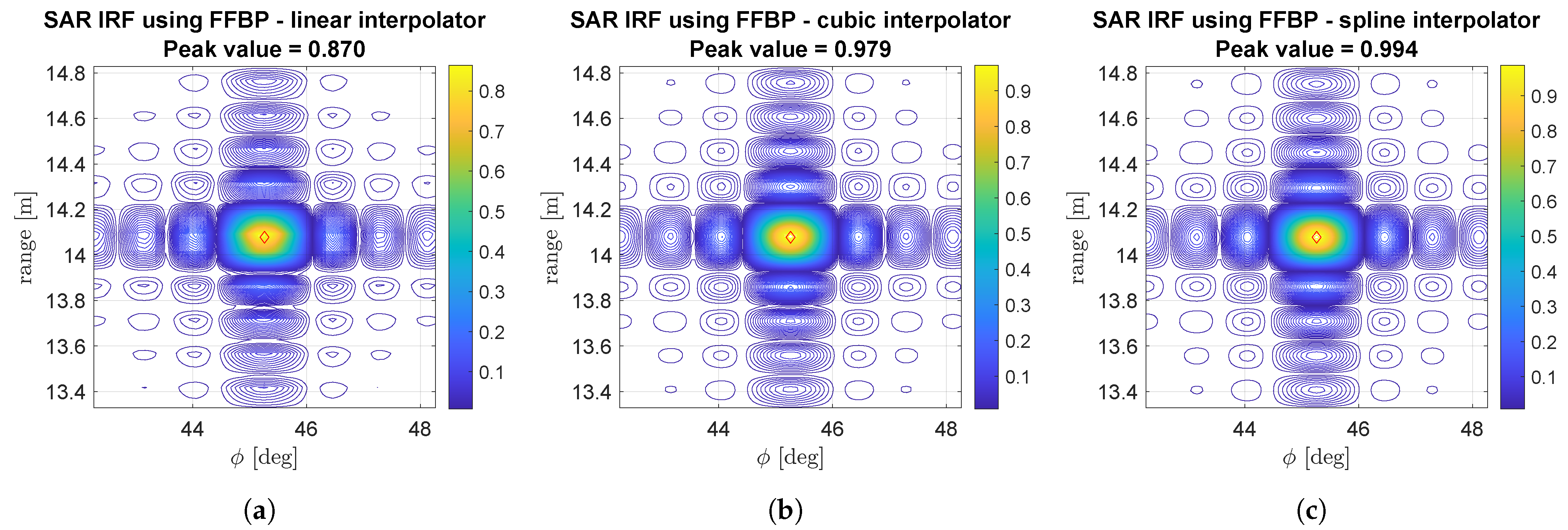
Figure 10, the FFBP has been tested using different interpolation kernels. In addition, in this case, the quality depends on the interpolation kernel used. The higher the degree of the interpolator, the better the image. The spline interpolator reaches practically the same accuracy of the direct TDBP.
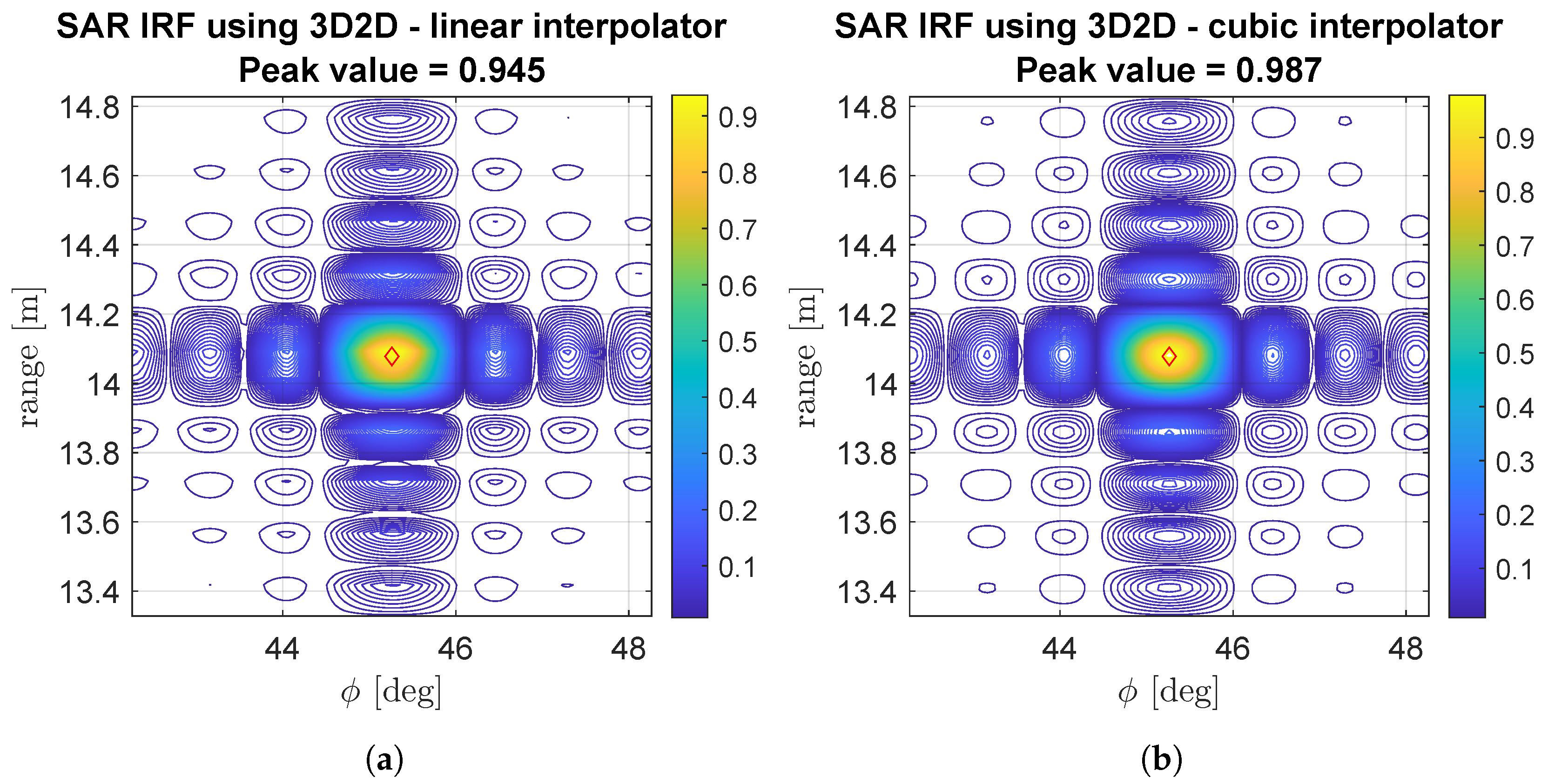
The same considerations on the interpolation kernel are valid for the 3D2D algorithm for which the IRF is depicted in
Figure 11. In this case, since the aperture is rather small, the linear approximation of Equation (
14) is valid; thus, the images are correctly placed in the baseband, and a correct imaging can take place. Using a cubic interpolator, the peak value of the IRF is just 0.11 dB lower than the optimal one.
Regarding the image quality, we deem that for short apertures, the two algorithms are comparable. If the processing units onboard the vehicle allow a fast implementation, it is better to use high-order interpolation kernels such as the spline and cubic interpolator.
4.2. Imaging with Longer Apertures
In this section, we compare again the two algorithms for different aperture sizes. The target is once again placed in m. In order to simulate different aperture sizes, we change the velocity of the vehicle while maintaining the PRF of the radar system as fixed. The tested velocities are:
m/s (108 km/h) leading to an aperture of 1.06 cm;
m/s (144 km/h) leading to an aperture of 1.45 m;
m/s (180 km/h) leading to an aperture of 1.82 m.
In
Figure 12, the three experiments are represented on each row, while the columns represent the different algorithms under test. For all the simulations, we used a cubic interpolator, since it is the one showing better performances.
From
Figure 12a,d,g, we see how the direct BP preserves the image quality even with longer apertures. This is an expected result, since the Time Domain Back-Projection is an exact algorithm that properly takes into account the range migration and non-linear nature of the phase.
Almost the same can be said for the FFBP (
Figure 12b,e,h). This algorithm always uses the true distances for demodulating and modulating the data; therefore, no image degradation happens for longer apertures. The 3D2D, on the other hand, is not able to properly handle the non-linearity of the phase with long apertures. The effect is clear from
Figure 12i where IRF is totally smeared.
In
Table 2, the normalized peak values of the IRF for each experiment are summarized.
The longer the aperture, the more the linear law used to baseband the low-resolution images is invalid. The approximated law of distances is more and more an approximation while we move at the extreme of the aperture. In
Figure 13, some demodulated spectra of low-resolution images in the stack are depicted. In
Figure 13a,d, the image at the center of the aperture is demodulated using the correct (hyperbolic) law and the approximated (linear) law of distances. It is clear that the two are exactly the same as expected. While we move toward the extremes of the aperture, the two spectra became more and more different, with a significant distortion happening for the ones demodulated using the approximated distance (see
Figure 13e,f).
Figure 12 provides a first quality metric for the IRF: the peak value. In
Table 3, the Integrated Side Lobes Ratio (ISLR) is also depicted. The ISLR [
15] is defined as:
where
is the total power of the IRF, while
is the power inside the main lobe.
The figure of merit confirms what is already clear: the 3D2D algorithm worsens for long apertures, reaching unacceptable values of ISLR for speed between 40 and 50 m/s.
We remark that all the proposed simulations use a single point target at almost 14 m of range. For the same angle
, but for longer ranges
r, the assumption on the phase linearity may hold even for long apertures, as shown in Equation (
21); thus, the image will be focused properly.
To conclude this section, we make some practical considerations for applying such algorithms in the automotive industry. Both algorithms work as expected for short aperture, leading to a well-focused and well-localized IRF. This is no longer the case for more extended aperture, since the 3D2D quickly loses the linear phase assumption, leading to bad performances. We deem, however, that such extreme aperture lengths are very often unnecessary: a synthetic aperture of just 0.5 cm leads to a resolution in the order of 0.3 deg around 45 deg, which is comparable with commercial LiDARs used in the automotive industry.
If extreme resolutions are necessary, a possible solution to preserve the image quality using the 3D2D approach is to divide the aperture into small sub-apertures where the phase can be considered linear; then, we combine these sub-apertures to obtain the full-resolution image.
5. Computational Costs: Rough Number of Operations and Processing Time
We now derive the computational burden of the two methods in terms of Rough Number of Operations (RNO). This figure of merit is tightly related to the computational time requested to form a full-resolution SAR image.
The objective of this section is to show that both the algorithms are suitable for real-time urban mapping.
5.1. Range Compression
In FMCW radars, the range compression is performed by a simple fast Fourier transform (FFT) of the demodulated and deramped raw data [
16]. The number of operations required by the FFT when the number of frequency points computed (
) is equal to a power of two is equal to
. The FFT must obviously be computed for each channel (
) and for each slow-time (
), leading to a total number of operations equal to:
In the following, we will give some indicative numbers providing a quantitative indication of the number of operations required by this step of the workflow.
5.2. Low-Resolution MIMO Image Formation
The second step is the TDBP of the range compressed data to form the stack of low-resolution snapshots of the scene. For each pixel in the BP grid, we need to:
- 1.
Calculate the bistatic distances from each real antenna phase center to the considered pixel. This operation is composed of six squares and two square roots (Pythagorean theorem) for a total of eight operations per channel.
- 2.
Interpolate the range compressed data using a linear or nearest neighbor interpolator accounting for two operations per channel.
- 3.
Modulate the signal, which is just a single complex multiplication per pixel.
- 4.
Accumulate the back-projected signal for each channel with a single complex summation.
We remark that these operations must be computed for each pixel in the BP grid and for each slow-time; thus, the final number of operations is equal to:
where
and
are the sizes of the polar BP grid in the range and angular direction, respectively, and the other symbols were already defined in the previous section.
5.3. FFBP Rough Number of Operations
As already discussed, the FFBP is divided into stages. In the first stage, we have slow-time snapshots, each one composed by samples in angle and samples in range. Each sub-aperture is composed by samples, leading to a set of sub-apertures.
The rough number of operations to be performed at the first stage of the FFBP can be expressed as:
where
is the number of sub-apertures;
is the number of samples for each sub-aperture;
expresses the number of pixels in the output grid from this stage which is proportional to the number of samples in the input grid () and the number of samples for each sub-aperture ();
is the number of pixels in range (it is constant since the interpolation is mono dimensional in angle);
K is the number of operations required to form each of the pixels in the output grid.
In the second stage, the number of samples for each sub-aperture remains the same, while the number of sub-apertures decreases by a factor of
. What instead increases is the number of angular samples of the output grid, which again increases by a factor of
. The resulting expression for the number of operations is then:
which is the same value of the first stage. It is now clear that the number of operations is constant for each stage of the FFBP, and it is equal to
The number of stages depends on the size of the initial set of snapshots (
) and on the size of each sub-aperture (
); thus, the total number of operations needed to form the final SAR image is:
In
Section 5.5, we provide some realistic figures for each parameter of Equation (
33). For what concerns the value of
K, instead, we can retrace the FFBP workflow and make a rough estimate of the number of operations requested per pixel:
- 1.
We first calculate the distance from the center of the virtual array to the pixel itself. This passage accounts for three squares and one square root (Pythagorean theorem).
- 2.
Demodulate the low-resolution images using the distances calculated in the previous step. This accounts for a single complex multiplication.
- 3.
Interpolate using a mono-dimensional interpolation in the angular direction that accounts for two or three operations, depending on the interpolation kernel.
- 4.
Compute again the distances, this time on the finer output BP grid. In addition, this time, we have a total of four operations.
- 5.
Modulate the interpolated images using the distances previously computed using a single complex multiplication.
By summing all the figures provided, we can state that the rough number of complex operations requested for each pixel is .
5.4. 3D2D Rough Number of Operations
The 3D2D algorithm starts again from the set of low-resolution MIMO images; thus, the number of operations required by the range compression and the initial TDBP are in common with the FFBP. The next step is a demodulation of each of the
low-resolution images. For each pixel, a single multiplication is performed to compute the distance Equation (
14) and a multiplication is performed to demodulate the data. This consideration leads to a number of operations equal to:
The next step is a slow-time FFT to be computed over each pixel, leading to:
where
is the number of frequency (or velocity) points computed by the FFT, a typical value is
.
The final step is the 3D interpolation. For each pixel of the output fine resolution polar grid, we have to compute the radial velocity (see Equation (
16)). This step requires a number of operations equal to the size of the output grid
where
is the size in the angular direction of the fine resolution polar grid.
Now, the interpolation takes place with a number of operations in the order of . The number 27 is derived from the fact that the current pixel is derived by combining the 27 closest neighbors, i.e., the cube centered on the pixel.
These considerations lead to a total number of operations equal to:
5.5. Comparison
In
Table 4, we provide some realistic values for the parameters described in the previous sections.
With these values, we can provide some quantitative results on the number of operations required by the two algorithms. We remark once again that it is not our intention to provide a accurate figure but rather just a rough order of magnitude.
Table 5 shows the number of operations (in millions, MM) for each one of the two algorithms.
Both the algorithms stay below half a billion of operations per image. For comparison, a 9-year-old iPhone®5S has a raw processing power of 76 GigaFlops, meaning it could focus an SAR image in 6 ms. We deem that with dedicated hardware such as FPGA/GPU, the urban scenario can be easily imaged in real time.
5.6. Processing Time on a Reference Machine
In this case, instead of focusing a small patch around the position of the target, we focus the entire visible scene as seen by the radar. In other words, the final polar grid will span an angle between −90 deg and +90 deg, and the range will go from the very near range ( m) to the far range ( m).
We used as a reference machine a Dell ®Precision 5820 with a 6 Core Intel Xeon W-2133. A summary of the computational performances is detailed in
Table 6. In this table, we compare the two algorithms with different aperture sizes
. In the parentheses, there is the processing time requested to form the low-resolution MIMO images, while it is outside the time requested by the algorithm itself.
With , the required time is basically the same, while for , the performances of the FFBP degrade, unlike the 3D2D that maintains almost the same processing time.
We remark also that the 3D2D can take advantage by fast GPU-based implementation of the FFT and 3D interpolation. Running the algorithm on an Nvidia Quadro P4000, we can cut the processing time by almost a factor of five.
This table includes all the best achievable performances with every algorithm (fastest interpolator and fastest sub-aperture size).
These processing times must be taken as reference time and will not reflect the real performances of a deploy-ready implementation.
6. Experimental Results with Real Data
In this section, we show the results from a few experimental campaigns carried out using a 77 GHz MIMO radar mounted in forward-looking mode on an Alfa-Romeo®Giulia Veloce.
The data are acquired by operating in burst mode with a duty cycle of 50% and transmitting chirp pulses with a bandwidth of 1 GHz. The PRF is about 7 kHz. The car is also fully equipped with navigation sensors to provide a rough estimate of the trajectory. We remark once again that the trajectory provided by the navigation unit is not sufficiently accurate and must be complemented by an autofocusing routine. Only in this way is it possible to achieve very high focusing and localization accuracy. To show its focusing performances in a real scenario, all the results provided in this section have been focused using the 3D2D processing scheme.
In
Figure 14, an example of processed aperture is depicted. On the top of the figure, an optical image is shown. At the bottom (central), an SAR image of the field of view is represented, while two zoomed details are shown on the left and the right. In the red rectangle, the parked cars to the vehicle’s left are highlighted, while on the right, the same green car visible in the optical image is also recognizable in the SAR image. The SAR images’ fine resolution allows recognition of even the smallest details, such as the green car’s alloy wheels.
Another example is the one depicted in
Figure 15. This experiment was carried out to test the capability of SAR images to behave as expected even in complex situations such as when a pedestrian is present on the roadway very close to parked cars. A target with a very high Radar Cross-Section (RCS), such as a parked vehicle, can hide a target with a low RCS (such as a pedestrian). This is not the case in SAR images, where the excellent resolution of the system guarantees the detection of both targets. In
Figure 15, a focused SAR image is shown on the left with some zoomed details on the bottom right and an optical image for reference. A row of parked cars is highlighted in the yellow box, while a free parking spot is depicted in the far field (green box). Notice how the resolution is degraded at boresight (i.e., in front of the car). The most important detail, however, is in the red box. A pedestrian is visible in the optical image, and it is easily detected also in the SAR image.
7. Conclusions
This paper aims to find the best algorithm to coherently combine low-resolution MIMO images to obtain a fine resolution SAR image. We deem that the generation of low-resolution images is a mandatory starting point for every vehicle-based SAR imaging algorithm. The reason is that such images allow for a simple and intuitive residual motion estimation, which in turn improves image quality and target localization accuracy.
We started with a theoretical review of the well-known Fast Factorized Back-Projection (FFBP), highlighting its strengths and weaknesses. We introduced the 3D2D scheme, detailing the algorithm itself and finding its theoretical limits regarding the aperture length. A possible alternative to the 3D2D called Quick&Dirty is also briefly described. It neglects range migration and phase curvature in favor of simpler processing.
We then proceed by making a comparison between the proposed schemes. We have compared several interpolation kernels and found that it is always better to use high-order interpolators such as cubic or spline, leading to higher-quality images with minimum additional computational cost.
We then compared the algorithms using longer apertures. In this scenario, the FFBP performs better than the 3D2D scheme. The reason is that while the former always uses the true law of distances for modulation/demodulation of the sub-images, the latter uses just a linear approximation. When apertures become long, the linearity hypothesis does not hold, leading to a deterioration of the image.
For the automotive industry, computational complexity is also a key factor. We provided a rough number of operations required by both processing schemes. The result is that both algorithms could run in real time if adequately implemented to work on dedicated hardware. The 3D2D/Q&D can also take particular advantage of GPU/FPGA implementation of the FFT.
While both algorithms are suited for a future real-world deployment, we deem that the 3D2D scheme is possibly simpler to implement, provides high-quality images, is generally faster, and can be easily transformed in an even faster scheme such as the Q&D. We proved that this processing scheme is suitable for an accurate imaging of the environment by showing results acquired in an open road campaign using a forward-looking 77 GHz MIMO radar.
Author Contributions
Conceptualization, M.M. and S.T.; methodology, M.M. and S.T.; software, M.M. and S.T.; validation, M.M.; formal analysis, M.M. and S.T.; investigation, M.M. and S.T.; resources, S.T., A.V.M.-G. and C.M.P.; data curation, M.M; writing—original draft preparation, M.M.; writing—review and editing, M.M., S.T. and A.V.M.-G.; visualization, M.M. and S.T.; supervision, S.T., A.V.M.-G., C.M.P. and I.R.; project administration, S.T., A.V.M.-G., C.M.P. and I.R.; funding acquisition, S.T., A.V.M.-G. and C.M.P. All authors have read and agreed to the published version of the manuscript.
Funding
This work is funded by Huawei Technologies Italia and has been carried out in the context of the activities of the Joint Lab by Huawei Technologies Italia and Politecnico di Milano.
Acknowledgments
We want to thank Dario Tagliaferri for processing navigation data and for being a great target in field campaigns.
Conflicts of Interest
Ivan Russo is a Huawei Technologies Italia S.r.l. employee.
References
- Saponara, S.; Greco, M.S.; Gini, F. Radar-on-Chip/in-Package in Autonomous Driving Vehicles and Intelligent Transport Systems: Opportunities and Challenges. IEEE Signal Process. Mag. 2019, 36, 71–84. [Google Scholar] [CrossRef]
- Ye, L.; Gu, G.; He, W.; Dai, H.; Lin, J.; Chen, Q. Adaptive Target Profile Acquiring Method for Photon Counting 3-D Imaging Lidar. IEEE Photonics J. 2016, 8, 1–10. [Google Scholar] [CrossRef]
- Wang, P.; Wang, L.; Leung, H.; Zhang, G. Super-Resolution Mapping Based on Spatial–Spectral Correlation for Spectral Imagery. IEEE Trans. Geosci. Remote Sens. 2021, 59, 2256–2268. [Google Scholar] [CrossRef]
- Li, J.; Stoica, P.; Zheng, X. Signal Synthesis and Receiver Design for MIMO Radar Imaging. IEEE Trans. Signal Process. 2008, 56, 3959–3968. [Google Scholar] [CrossRef]
- Tebaldini, S.; Manzoni, M.; Tagliaferri, D.; Rizzi, M.; Monti-Guarnieri, A.V.; Prati, C.M.; Spagnolini, U.; Nicoli, M.; Russo, I.; Mazzucco, C. Sensing the Urban Environment by Automotive SAR Imaging: Potentials and Challenges. Remote Sens. 2022, 14, 3602. [Google Scholar] [CrossRef]
- Stanko, S.; Palm, S.; Sommer, R.; Klöppel, F.; Caris, M.; Pohl, N. Millimeter resolution SAR imaging of infrastructure in the lower THz region using MIRANDA-300. In Proceedings of the 2016 46th European Microwave Conference (EuMC), London, UK, 4–6 October 2016; pp. 1505–1508. [Google Scholar] [CrossRef]
- Gishkori, S.; Daniel, L.; Gashinova, M.; Mulgrew, B. Imaging for a Forward Scanning Automotive Synthetic Aperture Radar. IEEE Trans. Aerosp. Electron. Syst. 2019, 55, 1420–1434. [Google Scholar] [CrossRef]
- Gishkori, S.; Daniel, L.; Gashinova, M.; Mulgrew, B. Imaging Moving Targets for a Forward Scanning SAR without Radar Motion Compensation. Signal Process. 2021, 185, 108110. [Google Scholar] [CrossRef]
- Farhadi, M.; Feger, R.; Fink, J.; Wagner, T.; Stelzer, A. Automotive Synthetic Aperture Radar Imaging using TDM-MIMO. In Proceedings of the 2021 IEEE Radar Conference (RadarConf21), Atlanta, GA, USA, 7–14 May 2021; pp. 1–6. [Google Scholar] [CrossRef]
- Laribi, A.; Hahn, M.; Dickmann, J.; Waldschmidt, C. Performance Investigation of Automotive SAR Imaging. In Proceedings of the 2018 IEEE MTT-S International Conference on Microwaves for Intelligent Mobility (ICMIM), Munich, Germany, 15–17 April 2018; pp. 1–4. [Google Scholar] [CrossRef]
- Feger, R.; Haderer, A.; Stelzer, A. Experimental verification of a 77-GHz synthetic aperture radar system for automotive applications. In Proceedings of the 2017 IEEE MTT-S International Conference on Microwaves for Intelligent Mobility (ICMIM), Nagoya, Japan, 19–21 March 2017; pp. 111–114. [Google Scholar] [CrossRef]
- Gao, X.; Roy, S.; Xing, G. MIMO-SAR: A Hierarchical High-Resolution Imaging Algorithm for mmWave FMCW Radar in Autonomous Driving. IEEE Trans. Veh. Technol. 2021, 70, 7322–7334. [Google Scholar] [CrossRef]
- Tagliaferri, D.; Rizzi, M.; Nicoli, M.; Tebaldini, S.; Russo, I.; Monti-Guarnieri, A.V.; Prati, C.M.; Spagnolini, U. Navigation-Aided Automotive SAR for High-Resolution Imaging of Driving Environments. IEEE Access 2021, 9, 35599–35615. [Google Scholar] [CrossRef]
- Manzoni, M.; Tagliaferri, D.; Rizzi, M.; Tebaldini, S.; Monti-Guarnieri, A.V.; Prati, C.M.; Nicoli, M.; Russo, I.; Duque, S.; Mazzucco, C.; et al. Motion Estimation and Compensation in Automotive MIMO SAR. arXiv 2022, arXiv:2201.10504. [Google Scholar]
- Cumming, I.G.; Wong, F.H.c. Digital Processing of Synthetic Aperture Radar Data: Algorithms and Implementation; Artech House Remote Sensing Library, Artech House: Boston, MA, USA, 2005. [Google Scholar]
- Meta, A.; Hoogeboom, P.; Ligthart, L.P. Signal Processing for FMCW SAR. IEEE Trans. Geosci. Remote Sens. 2007, 45, 3519–3532. [Google Scholar] [CrossRef]
- Ulander, L.; Hellsten, H.; Stenstrom, G. Synthetic-aperture radar processing using fast factorized back-projection. IEEE Trans. Aerosp. Electron. Syst. 2003, 39, 760–776. [Google Scholar] [CrossRef]
- Frey, O.; Magnard, C.; Ruegg, M.; Meier, E. Focusing of Airborne Synthetic Aperture Radar Data From Highly Nonlinear Flight Tracks. IEEE Trans. Geosci. Remote Sens. 2009, 47, 1844–1858. [Google Scholar] [CrossRef]
- Tebaldini, S.; Rocca, F.; Mariotti d’Alessandro, M.; Ferro-Famil, L. Phase Calibration of Airborne Tomographic SAR Data via Phase Center Double Localization. IEEE Trans. Geosci. Remote Sens. 2016, 54, 1775–1792. [Google Scholar] [CrossRef]
- Pinto, M.A.; Fohanno, F.; Tremois, O.; Guyonic, S. Autofocusing a synthetic aperture sonar using the temporal and spatial coherence of seafloor reverberation. In Proceedings of the High Frequency Seafloor Acoustics (SACLANTCEN Conference Proceedings CP-45), Lerici, Italy, 30 June–4 July 1997; pp. 417–424. [Google Scholar]
- Prats, P.; de Macedo, K.A.C.; Reigber, A.; Scheiber, R.; Mallorqui, J.J. Comparison of Topography- and Aperture-Dependent Motion Compensation Algorithms for Airborne SAR. IEEE Geosci. Remote Sens. Lett. 2007, 4, 349–353. [Google Scholar] [CrossRef]
- Tebaldini, S.; Rizzi, M.; Manzoni, M.; Guarnieri, A.M.; Prati, C.; Tagliaferri, D.; Nicoli, M.; Spagnolini, U.; Russo, I.; Mazzucco, C.; et al. A Quick and Dirty processor for automotive forward SAR imaging. In Proceedings of the 2022 IEEE Radar Conference (RadarConf22), New York City, NY, USA, 21–25 March 2022; pp. 1–6. [Google Scholar] [CrossRef]
Figure 1.
Geometry of the system. The red dots are the virtual channels of the MIMO radar with a distance d, is the azimuth angle, and the black dot is a generic location is the field of view. In this figure, the installation angle is deg, representing a forward-looking geometry (a,b).
Figure 1.
Geometry of the system. The red dots are the virtual channels of the MIMO radar with a distance d, is the azimuth angle, and the black dot is a generic location is the field of view. In this figure, the installation angle is deg, representing a forward-looking geometry (a,b).
Figure 2.
Fixed polar grid where the signal is back-projected. Notice that this grid is strictly polar just for the last acquisition where the origin of the grid is co-located with the center of the virtual array.
Figure 2.
Fixed polar grid where the signal is back-projected. Notice that this grid is strictly polar just for the last acquisition where the origin of the grid is co-located with the center of the virtual array.
Figure 3.
Block diagram of the FFBP algorithm.
Figure 3.
Block diagram of the FFBP algorithm.
Figure 4.
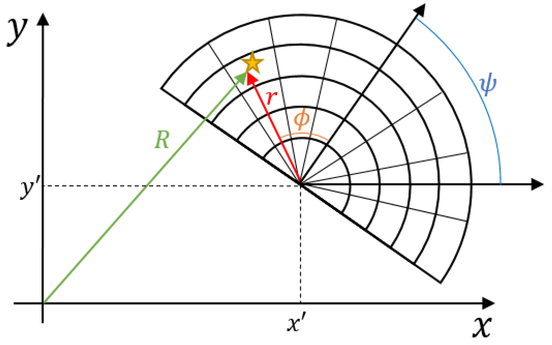
Roto-translated back-projection polar grid. The grid is centered in coordinates and , and it is rotated with an angle with respect to the Cartesian reference. The TX/RX antenna is located in the origin of the Cartesian reference. The target is represented by the yellow star.
Figure 4.
Roto-translated back-projection polar grid. The grid is centered in coordinates and , and it is rotated with an angle with respect to the Cartesian reference. The TX/RX antenna is located in the origin of the Cartesian reference. The target is represented by the yellow star.
Figure 5.
Block diagram of the 3D2D algorithm.
Figure 5.
Block diagram of the 3D2D algorithm.
Figure 6.
Range-Angle-Doppler data cube with three constant Doppler planes depicted.
Figure 6.
Range-Angle-Doppler data cube with three constant Doppler planes depicted.
Figure 7.
On the bottom of the plot, the radar image is computed by detecting the maximum Doppler for each range-angle bin. The SAR image can be interpreted as an intersection of the 3D RAV cube with a 2D surface.
Figure 7.
On the bottom of the plot, the radar image is computed by detecting the maximum Doppler for each range-angle bin. The SAR image can be interpreted as an intersection of the 3D RAV cube with a 2D surface.
Figure 8.
Block diagram of the Quick&Dirty (Q&D) algorithm.
Figure 8.
Block diagram of the Quick&Dirty (Q&D) algorithm.
Figure 9.
cm. SAR Impulse Response Function (IRF) generated by direct TDBP on a very fine polar grid centered in the nominal position of the target. The higher the order of the interpolator, the better the image in terms of peak value and side lobes.
Figure 9.
cm. SAR Impulse Response Function (IRF) generated by direct TDBP on a very fine polar grid centered in the nominal position of the target. The higher the order of the interpolator, the better the image in terms of peak value and side lobes.
Figure 10.
cm. SAR ImpulseResponse Function (IRF) generated by FFBP on a very fine polar grid centered in the nominal position of the target. The higher the order of the interpolator, the better the image in terms of peak value and sidelobes.
Figure 10.
cm. SAR ImpulseResponse Function (IRF) generated by FFBP on a very fine polar grid centered in the nominal position of the target. The higher the order of the interpolator, the better the image in terms of peak value and sidelobes.
Figure 11.
cm. SAR Impulse Response Function (IRF) generated by 3D2D on a very fine polar grid centered in the nominal position of the target. The higher the order of the interpolator, the better the image in terms of peak value and sidelobes.
Figure 11.
cm. SAR Impulse Response Function (IRF) generated by 3D2D on a very fine polar grid centered in the nominal position of the target. The higher the order of the interpolator, the better the image in terms of peak value and sidelobes.
Figure 12.
IRF with different aperture size. (First row) m. (Second row) m. (Third row) m. All the IRF are focused on using a cubic interpolator.
Figure 12.
IRF with different aperture size. (First row) m. (Second row) m. (Third row) m. All the IRF are focused on using a cubic interpolator.
Figure 13.
Baseband spectra of some low-resolution MIMO images. The row on top shows the spectra demodulated with the true (hyperbolic) law of distances. The row on the bottom shows the spectra demodulated with the approximated (linear) low of distances. In the left column, the spectra of the image in the middle of the aperture are represented. In this case, the linear approximation matches perfectly the true distance. Moving away from the center of the aperture (second and third columns), the spectra start to be more and more aliased, leading to a degradation of the final SAR image.
Figure 14.
(top) Optical image of the field of view. (bottom central) SAR image of the entire scenario. (bottom right) A detail of the full SAR image: the green car in the optical image is parking. (bottom left) Another detail: some parked cars to the left of the vehicle.
Figure 14.
(top) Optical image of the field of view. (bottom central) SAR image of the entire scenario. (bottom right) A detail of the full SAR image: the green car in the optical image is parking. (bottom left) Another detail: some parked cars to the left of the vehicle.
Figure 15.
(left) SAR image of the field of view: (top right) Optical image. (bottom right) Three details of the SAR image highlighted with the some color in the optical image and in the full-field SAR image.
Figure 15.
(left) SAR image of the field of view: (top right) Optical image. (bottom right) Three details of the SAR image highlighted with the some color in the optical image and in the full-field SAR image.
Table 1.
Parameters of the simulated radar and vehicle.
Table 1.
Parameters of the simulated radar and vehicle.
| Parameter | Value |
|---|
| Bandwidth (B) | 1 GHz |
| Number of virtual channels () | 8 |
| PRF | 7 KHz |
| Number of pulses forming an aperture | 256 |
| Simulated vehicle velocities (v) | 5, 30, 40, 50 m/s |
| Mode | Forward looking |
Table 2.
Normalized peak values of the IRF for different velocities (aperture length) and for different focusing algorithms.
Table 2.
Normalized peak values of the IRF for different velocities (aperture length) and for different focusing algorithms.
| | m/s | m/s | m/s |
|---|
| Direct TDBP | 0.987 | 0.987 | 0.987 |
| FFBP | 0.975 | 0.940 | 0.952 |
| 3D2D | 0.957 | 0.881 | 0.561 |
Table 3.
ISLR for different velocities (aperture length) and for different focusing algorithms.
Table 3.
ISLR for different velocities (aperture length) and for different focusing algorithms.
| | m/s | m/s | m/s | m/s |
|---|
| Direct BP | dB | dB | dB | dB |
| FFBP | dB | dB | dB | dB |
| 3D2D | dB | dB | dB | dB |
Table 4.
List of the parameters involved in the calculation of the total number of operations requested to form an SAR image.
Table 4.
List of the parameters involved in the calculation of the total number of operations requested to form an SAR image.
| Parameter | Description | Typical Value |
|---|
| Number of fast time samples | 512 |
| Number of frequency samples after range compression | 1024 |
| Number of slow-times samples for each aperture | 256 |
| Number of MIMO channels | 8 |
| Number range samples in the polar BP grid | 400 |
| Number angular samples in the low-res polar BP grid | 17 |
| Number angular samples in the fine resolution polar BP grid | 2048 |
| Sub-aperture size | 2 |
| Number of velocity points for 3D2D | 2048 |
Table 5.
Rough number of operations required to form an SAR image using the two described algorithms.
Table 5.
Rough number of operations required to form an SAR image using the two described algorithms.
| Processing Block | Range Compression | TDBP | SAR Focusing | Total |
|---|
| FFBP | 21 MM | 148 MM | 298 MM | 467 MM |
| 3D2D | 21 MM | 148 MM | 159 MM | 329 MM |
Table 6.
Processing times for different algorithms. All the numbers are in seconds.
Table 6.
Processing times for different algorithms. All the numbers are in seconds.
| | | |
|---|
| Direct BP | 72.93 | 148.82 |
| FFBP | 0.42 (+1.07) | 0.68 (+2.02) |
| 3D2D | 0.43 (+1.07) | 0.48 (+2.02) |
| 3D2D (GPU) | 0.11 (+1.07) | 0.19 (+2.02) |
| Publisher’s Note: MDPI stays neutral with regard to jurisdictional claims in published maps and institutional affiliations. |
© 2022 by the authors. Licensee MDPI, Basel, Switzerland. This article is an open access article distributed under the terms and conditions of the Creative Commons Attribution (CC BY) license (https://creativecommons.org/licenses/by/4.0/).


 ,
, 


