Abstract
Domain adaptation for classification has achieved significant progress in natural images but not in remote-sensing images due to huge differences in data-imaging mechanisms between different modalities and inconsistencies in class labels among existing datasets. More importantly, the lack of cross-domain benchmark datasets has become a major obstacle to the development of scene classification in multimodal remote-sensing images. In this paper, we present a cross-domain dataset of multimodal remote-sensing scene classification (MRSSC). The proposed MRSSC dataset contains 26,710 images of 7 typical scene categories with 4 distinct domains that are collected from Tiangong-2, a Chinese manned spacecraft. Based on this dataset, we evaluate several representative domain adaptation algorithms on three cross-domain tasks to build baselines for future research. The results demonstrate that the domain adaptation algorithm can reduce the differences in data distribution between different domains and improve the accuracy of the three tasks to varying degrees. Furthermore, MRSSC also achieved fairly results in three applications: cross-domain data annotation, weakly supervised object detection and data retrieval. This dataset is believed to stimulate innovative research ideas and methods in remote-sensing cross-domain scene classification and remote-sensing intelligent interpretation.
1. Introduction
Remote-sensing scene classification aims to predict the semantic category of image blocks by mining the visual primitives in a remote-sensing image scene (image block) and the spatial relationship between visual primitives [1,2]. It can greatly reduce the confusion of pixel-level or object-level ground object interpretation and improve the stability and accuracy of remote-sensing image interpretation. It has important application value in content-based remote-sensing image retrieval and remote-sensing target detection [3,4].
In the field of remote sensing, the data discrepancies between the source domain and the target domain are often caused by differences in imaging time, imaging atmospheric conditions, imaging locations and imaging sensors [5,6]. In this case, the classifier trained directly from the source domain data cannot achieve the desired results in the target domain. Therefore, a model trained on a specific dataset (source domain) is often difficult to generalize to another image set (target domain) that the model has not seen in the training process [5]. Moreover, to solve the domain adaptation problem by directly fine tuning the model in the target domain, it is very time-consuming and laborious to collect the corresponding labels, and the in-orbit intelligent application is also limited. At present, with the increases in satellites and various sensors, the number and types of remote-sensing images available are becoming increasingly diverse. It is unrealistic to build datasets and fine tune models for massive new multisource data and tasks. An effective method is urgently needed for solving the generalization problem of remote-sensing images from source domain to target domain, which is to provide not only efficient solutions for subsequent tasks but also a feasible method of breaking through the barriers between existing datasets and achieving larger-scale applications.
The traditional method is to label a small amount of new data and fine tune the network trained in the source domain to adapt to the new data, which is not only time-consuming and laborious but also challenging in that the target domain data usually have the characteristics of difficult acquisition, small amount of data and difficult labeling. Additionally, for problems with large domain differences, such as using the model trained on the visible dataset for the shortwave infrared, thermal infrared, and even synthetic aperture radar (SAR) data for model reasoning, the model often fails to achieve good results. For tasks with no label in the target domain and great differences between the source domain and the target domain, the mainstream method is domain adaptation, which can improve the performance of the tasks in the target domain by reducing the differences in the characteristic distribution between the source domain and the target domain. In order to reduce the differences in feature distribution between the source domain and target domain, the research focus of the domain adaptation algorithm is how to correct the feature distribution of source domain and target domain without changing the important attributes of the specific data, so that a classifier trained only by source domain data can be directly applied to target domain data and achieve satisfactory classification results.
Domain adaptation algorithms have become one of the popular research topics in the field of computer vision. The research in the field of remote sensing is relatively lagging. Datasets are an important driver and promoter of their development. Currently, most of the public remote-sensing scene classification datasets are optical remote-sensing images, while few scene classification datasets are based on radar images, short-wave infrared images and thermal infrared images. Because of their special imaging mechanisms, radar data, short-wave infrared data and thermal infrared data have their own characteristics that are complementary to optical images. Therefore, it is of great significance and value to construct domain-adaptive remote-sensing scene classification datasets including visible light, radar, short-wave infrared and thermal infrared images.
In this paper, we extend the preliminary version of MRSSC, i.e., MRSSC 1.0 [7], to MRSSC2.0. Specifically, MRSSC2.0 collects 26,710 scene images from a wide-band imaging spectrometer (WIS) and an interferometric imaging radar altimeter (InIRA) on Tiangong-2 and contains 7 categories from 4 domains. Ten domain adaptation methods are evaluated, and three applications are expanded, which is helpful for verifying the domain migration performance of data between different modes and exploring the innovative application of domain adaptation in remote sensing. This study will provide a data source for researchers to carry out the application research of domain transfer learning based on artificial intelligence and remote-sensing images, provide strong support for the transfer learning of remote sensing scene classification datasets and promote the deep fusion application of multiple remote-sensing scene classification datasets.
2. Related Works
2.1. Scene Classification Datasets
Scene recognition (scene classification) usually refers to common semantic analysis and image understanding, which is one of the landmark tasks in computer vision. On the basis of object recognition, scene classification can combine context information to achieve accurate recognition of the main content of a scene. Since 2006, the learning ability of neural networks has been improving continuously. Efficient deep learning models based on convolutional neural networks have been widely used in remote-sensing image applications. The training of a neural network depends on a large number of labeled samples. Therefore, many remote-sensing image classification datasets have been developed and released, including UC Merged [8], AID [2], BigEarthNet [9] and NaSC-TG2 [10]. These datasets are mainly aimed at typical scenes in urban areas, and the images are RGB images in aerial visible light.
Published multimodal scene classification datasets rarely use short-wave infrared and thermal infrared. However, some researchers have disclosed multimodal datasets of Optics and SAR, which are used to carry out research on image matching, image conversion and other topics. Wang et al. [11] present a dataset called SARptical that contains SAR and optical images of dense urban areas for image matching. The WHU-SEN-City dataset, proposed by Wang et al. [12], covers 32 Chinese cities and is used for SAR-to-optical-image conversion research. These multimodal datasets mainly contain urban scene images in pairs with single scene type, which can hardly support domain adaptation research in remote-sensing scene classification.
To study the domain adaptation classification algorithms, datasets with different distribution between the source domain and the target domain are required. Current public datasets commonly used in computer vision include Office-31 [13] and VisDA-2017 [14]. Most of the research on domain adaptation in remote sensing used the published scene classification datasets for cross-domain experiments. The data used in the experiment are as follows: the source domain and the target domain are single-mode (three channel) remote-sensing images from different regions or sensors, and the source domain and the target domain have not only distribution discrepancy but also category incompleteness [5,6]. These studies are based on the published remote-sensing scene classification dataset with single mode (three channels), and the data distribution has little difference. Our preliminary work, MRSSC1.0 [7], presented a dataset with seven categories and two domains, allowing for efficiently training robust domain adaptation models for remote-sensing cross-domain scene classification for the first time.
2.2. Domain Adaptation Algorithms
Domain adaptation (DA) aims to achieve the effect that the performance of the model in the target domain approximates or even maintains in the original domain, that is, to introduce some means of reducing the gap between the two domains in the feature space and eliminating the domain shift as much as possible, so that the model can learn more universal and domain-invariant features. DA is a kind of transfer learning to solve tasks when the target domain has no label and the source domain is quite different from the target domain. In the task of daily image scene classification, the research of domain adaptation has made great progress. These methods can be roughly divided into discrepancy-based, adversarial-based and theory-inspired.
Discrepancy-based methods aim to achieve the alignment of feature distributions in different domains by minimizing the statistical distance between the source domain and the target domain. Tzeng et al. [15] designed a deep domain confusion (DDC) scheme by adding the adaptive metric to the penultimate layer of the classification network, which can measure the distance between distributions with maximum mean discrepancy (MMD) [16]. Based on the DDC method, Long et al. [17] added three adaptive layers and adopted multicore MMD indicators with better characterization ability, which improved the accuracy of cross-domain remote-sensing classification. Long et al. [18]. proposed a joint adaptation network (JAN) to adjust the multilayer joint distribution. Xu et al. [19] used step-by-step adaptive feature norms to learn task-specific features with large norms in a progressive manner. Minimum class confusion (MCC) proposed by Jin et al. [20] can minimize category confusion in multifunctional domain-adaptive target prediction.
Adversarial-based methods use a discriminator to distinguish the data domain while learning the feature extraction program that may confuse the discriminator, finally learning the features with small influence of domain differences and large differences between categories. The domain-adversarial neural network (DANN) was introduced by the authors of [21], who introduced a domain discriminator to encourage feature extractors to learn domain-independent features. On the basis of DANN, a series of methods were derived such as conditional domain antagonism network (CDAN) [22], maximum classifier difference (MCD) [23], source domain and target domain through different mappings to achieve aligned adversarial discriminative domain adaptation (ADDA) [21] and batch spectral penalization (BSP) [24].
Theory-inspired methods refer to algorithma that can explicitly control the generalization error of transfer learning through strict theoretical derivation such as interval divergence method of margin disparity discrepancy (MDD) [25].
This paper will fully test the performance of the above methods on MRSSC in order to provide reference for subsequent research.
3. Materials and Methods
3.1. Images Collection
Data with different imaging mechanisms were the basis for constructing domain-adaptive datasets. The Tiangong-2 space laboratory is equipped with a wide-band imaging spectrometer (WIS) and a interferometric imaging radar altimeter (InIRA), which can obtain visible near infrared (VIS), short wavelength infrared (SWI), thermal infrared (INF) and SAR images [26]. For VIS, SWI and INF, the spectral ranges were 0.4~1.0 μm, 1.0~1.7 μm and 8.0~10.0 μm; the channel numbers were 14, 2 and 2; the spatial resolutions were 100 m, 200 m and 400 m; and the accuracies of absolute radiation calibration were 10%, 10% and 2 K, respectively [10]. For InIRA, the working frequency was 13.58 GHz, the work bandwidth was 40 MHz, the certainty of backscatter sounding was less than 2.0 dB and the spatial resolution of the two-dimensional images was 40 × 40 m. In addition, there were high-resolution two-dimensional images and DEM of InIRA that were been included in this dataset [27]. WIS and InIRA provide multilevel data products, of which the level-2 product of WIS was processed by field-of-view spreading, interband registration, nonuniformity correction, radial correction, sensor correction and geometric correction, and the level-2 product of InIRA was processed by imaging processing, azimuth multiview processing, radiometric correction and geometric correction to form a two-dimensional image product with map projection. The above data had domain differences with high quality, providing rich data sources for MRSSC. In order to improve the diversity of data, we carefully selected data from different regions, imaging times and imaging conditions.
3.2. Categories Selection
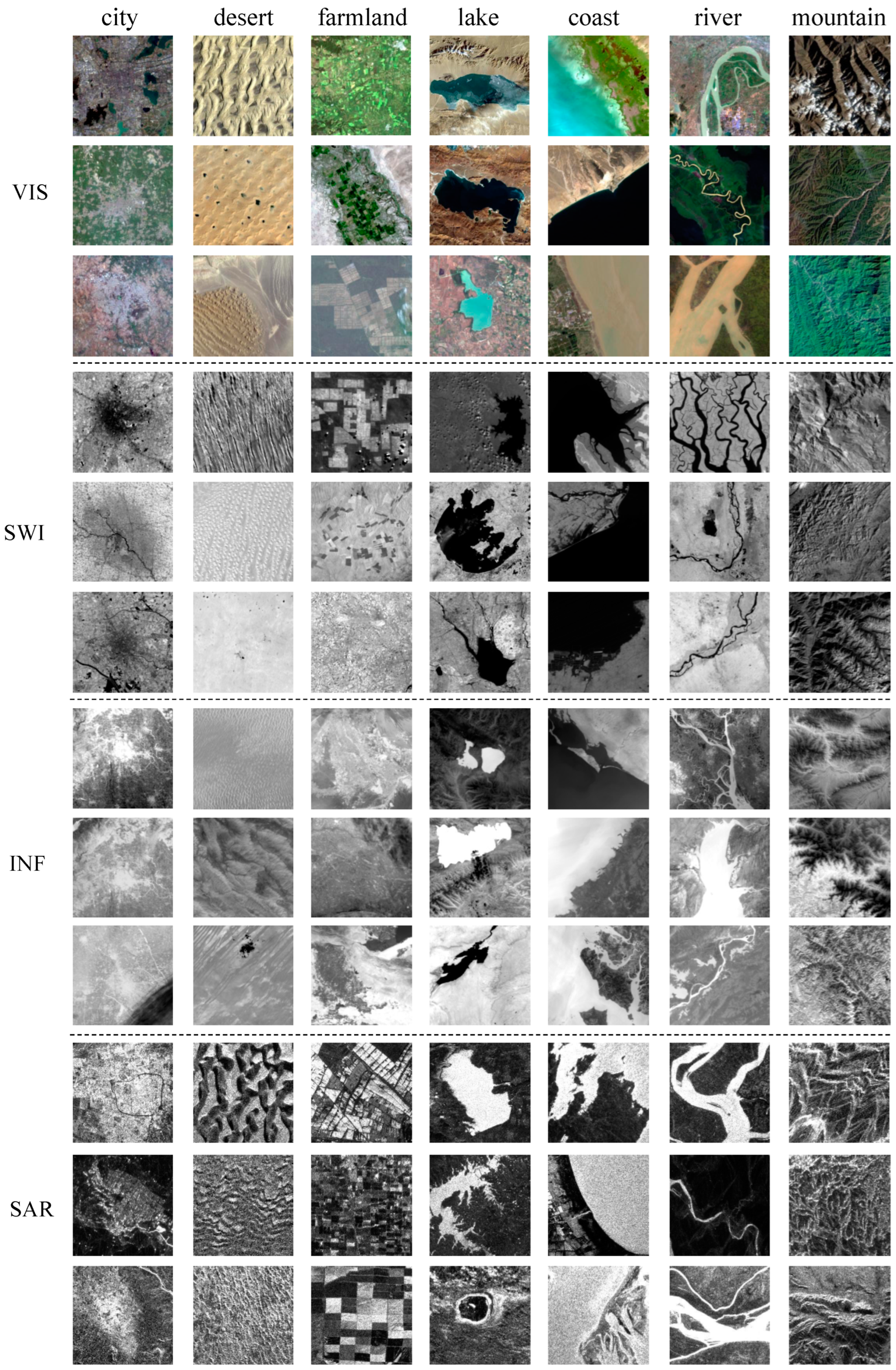
Seven categories were chosen and annotated in our MRSSC2.0 dataset, including river, lake, city, farmland, mountain, coast and desert, as shown in Figure 1.
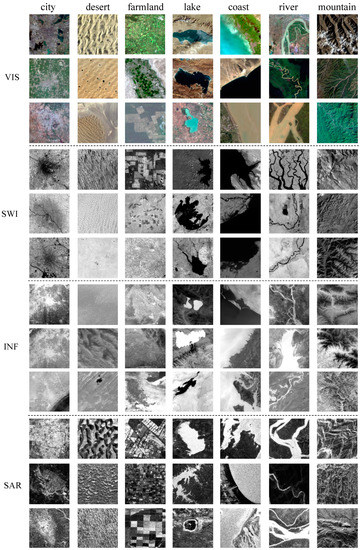
Figure 1.
Examples images of MRSSC2.0 dataset.
The categories were selected according to the characteristics of data and the value for real-world applications. The spatial resolutions of VIS, SWI, INF and SAR were medium, so the scene category settings were as consistent as possible with the land cover classifications. The advantage of this is that in the application scenario of in-orbit intelligent analysis, the relatively large-scale scene classification helps to quickly analyze and understand the semantics of the in-orbit push scan data. Combined with the fine target detection method, it realizes in-orbit real-time analysis at the subsecond level and provides support for the application scenario of intelligent processing, storage and downlink.
3.3. Annotation Method
Data Clipping. The dataset was obtained by professional remote-sensing experts through manual cutting. In order to ensure that the image label could reflect the image content, the main object was located in the middle of the image and accounted for a large proportion or conformed to the attention mechanism.
Considering the information content of the scene, spatial resolution and adaptability of the algorithm, the image size in MRSSC was 256 × 256 pixels for the four domain images. The resolutions of the four domain data were different, so the scenes had scale differences. For coastal, desert and mountain, the images affected by scale were small. For other scenes, objects of different scales were selected to make up for this difference. For example, the lake scale selected in VIS was smaller, while the lake scale selected in SWI and INF was larger, both to ensure that the cropped image could represent the overall scene.
Band Selection. VIS was a RGB true color image (R: 0.655~0.675 μm, G: 0.555~0.575 μm, B: 0.480~0.500 μm), SWI was a gray image (1.23~1.25 μm), INF is gray image (8.125~8.825 μm), and SAR was a two-dimensional image. Different types of data had different imaging mechanisms, resulting in different data distributions. VIS truly reflected the surface state, SWI was more sensitive to soil moisture, INF reflected the surface temperature state and SAR reflected the degree of surface backscattering.
3.4. Dataset Splits
In order to test the mobility between different data, we took VIS as the source domain and SWI, INF and SAR as the target domains. The MRSSC2.0 dataset was divided into seven parts: one source domain, three target domains and three test sets. There were no data intersections between the target domain and the test set. The source domain included VIS images, and the target domains were SWI, INF and SAR images, respectively represented by the numbers 1, 2, and 3. Target and test were divided by 4:1. The images in the source domain contained labels for training, while the images in target domain did not have labels and were used for domain adaption. The image numbers in each of the seven category are shown in Table 1.

Table 1.
Division of MRSSC2.0 dataset.
3.5. MRSSC Versions
It is important to note the significant improvements from MRSSC1.0 to MRSSC2.0. MRSSC1.0 only included two data types, VIS and SAR, while MRSSC2.0 expanded the modals to four by adding SWI and INF data. In many application scenarios, the domain adaptation problem of VIS and INF is very common. In addition, studying the domain migration characteristics between four types of data provided a reference for the application of unsupervised cross-domain scene classification.
3.5.1. MRSSC1.0
MRSSC1.0 contains 2 domains, 7 categories and 12,167 images. The source domain consisted of all labeled VIS data, the target domain consisted of unlabeled SAR data and the test set consisted of labeled SAR data (100 pieces per category). The ource and target domains were used for model training, and the test sets were used for model testing [7].
3.5.2. MRSSC2.0
There were 4 domains, 7 common categories and 26,710 images in MRSSC2.0. Compared with MRSSC1.0, two new domains, SWI and INF, were added. The MRSSC2.0 data were split into source domain, target domain and test set. The source domain consisted of the entire VIS dataset, and the target domain consisted of the SWI, INF and SAR data separately. In order to keep the division of target domain consistent, the division ratio of target domain to test set was 4:1. In addition, in order to verify the domain adaptation weakly supervised localization, an additional dataset for application tasks was provided.
3.6. Properties of MRSSC Dataset
3.6.1. Large Domain Differences Due to Different Imaging Mechanisms
The imaging mechanisms of a wide-band imaging spectrometer (WIS) and an interferometric imaging radar altimeter (InIRA) are very different. The WIS obtains image data using visible light and some infrared band sensors, while the InIRA uses microwave band (Ku band) sensors. WIS contains gray information of multiple bands for target recognition and classification extraction, while InIRA only records the echo information of one band and then extracts the corresponding amplitude and phase information through transformation. The amplitude information usually corresponds to the backscattering intensity of radar waves from ground targets and is closely related to the medium, water content and roughness. Additionally, the signal-to-noise ratio of SAR images is low, and there are unique geometric distortions such as overlay, perspective shrinkage and multipath false targets.
The three data products of wide-band imaging spectrometer, VIS, SWI and INF, also show certain differences due to the differences in imaging bands. SWI uses light reflection imaging, which is similar to the principle of visible light imaging. The difference is that the band of SWI can “bypass” the small particles in smoke, fog and haze and has better detail resolution and analysis ability. INF uses radiant thermal imaging to reflect the temperature difference of ground object surface and can be used for night imaging or smoke and fog scene imaging.
These multimodal data have strong complementarity and domain differences in data distribution, which is challenging for research on multimodal remote-sensing image scene understanding.
3.6.2. Large Domain Differences Caused by Scale Differences
The resolutions of VIS, SWI, INF and SAR were 100, 200, 400 and 40 m, respectively, and the sizes were almost all 256 × 256. Following the principle of dataset production, there were scale differences among the final cut categories. For example, the domain with low resolution selected larger cities, while the domain with high resolution selected smaller cities, to ensure that the target category occupied the main position of the image.
In addition, in order to increase the data richness, the intra-class differences, the classification difficulty and the model robustness, we selected different-scale images in the same category, such as rivers, including wide, medium-sized and narrow rivers.
3.6.3. Large Domain Differences Due to Different Imaging Time
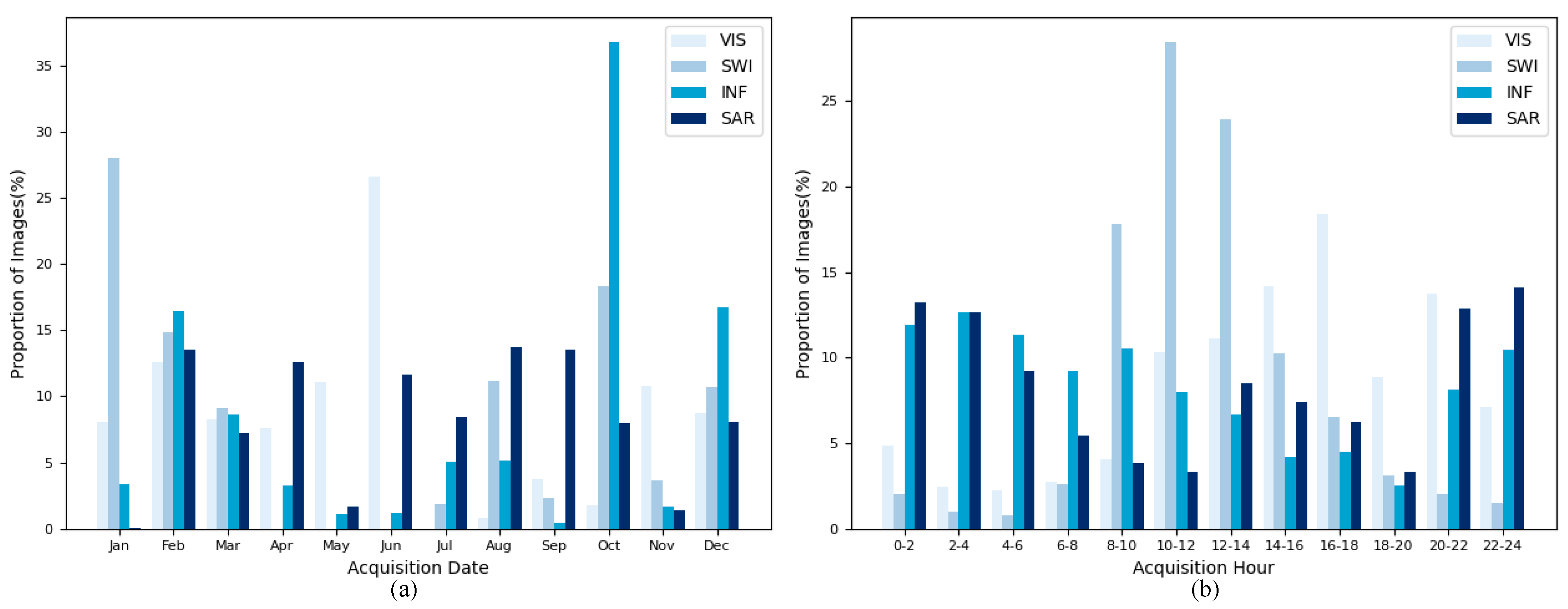
The imaging times of VIS, SWI, INF and SAR were different. The imaging times of VIS and SWI were relatively short, only in the daytime, while INF and SWI could be imaged all day.
In addition, in order to increase the date richness, we selected data from different phases, including different seasons and different imaging times. Statistic results of acquisition time are shown in Figure 2, and the intra-class differences are helpful for extracting richer class features and improving the model robustness.
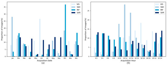
Figure 2.
Proportion of MRSSC2.0 images on (a) acquisition date, (b) acquisition hour.
3.6.4. Large Domain Differences Caused by Different Imaging Areas
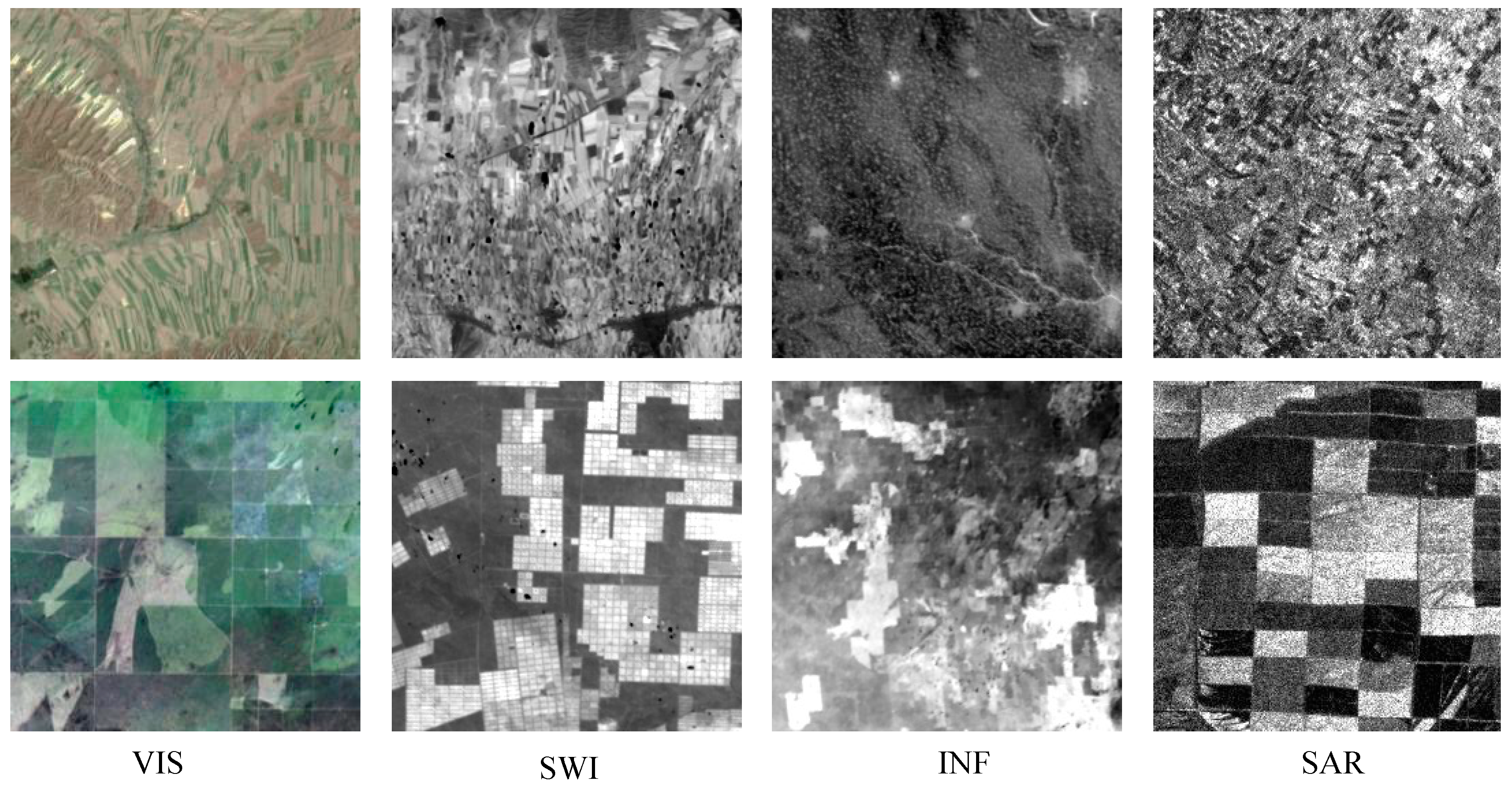
MRSSC2.0 contains images of different regions within 42 degrees of north–south latitude, not limited to specific countries, cities or scene types, with rich spatial differences. Due to the differences in spatial locations, there are differences in the data distributions of the same scene among the four data domains of MRSSC2.0 in color, shape, texture, etc. In addition, there are large differences within the same scene category, such as farmland with large blocks and regular shapes and farmland with small pieces and different shapes, as shown in Figure 3. This increased the challenge of the domain adaptation algorithm, prevented overfitting and improved the model performance.

Figure 3.
Examples of farmland categories in different domains.
4. Benchmark Results
4.1. Problem Setting
Due to the abundance of visible image data, it is mature to use visible image to realize remote-sensing scene classification. How to use visible image classifier for short-wave infrared, thermal infrared and SAR data scene classification is a research topic that needs to be solved.
Due to the domain differences caused by different sensors, the data distribution does not meet the consistency assumption that the training data and test data are distributed in the same feature space in machine learning, so it is impossible to achieve good classification results in the target domain. To solve this problem, we could consider using more optical images to train a scene classifier, adjust the knowledge learned in one domain (called the source domain) through domain adaptation (DA) and apply it to another related domain (called the target domain). By reducing the differences in the data and feature distribution between the source domain and the target domain, the model trained in the source domain could work normally in the target domain.
The source domain set was labeled VIS data, and the target domain set consisted of three unlabeled multimodal datasets: SWI, INF and SAR data. The corresponding tests of labeled SWI, INF and SAR were used for model evaluation. The rest of experiments in this section investigated the following questions: (1) Can DA increase the scene classification accuracy compared with source-only approaches, which directly test the classification model trained by optical images on unlabeled data? (2) Which DA methods perform better in the case of large appearance differences between source and target data? (3) What are the differences in the effects of DA between different source–target data?
4.2. Evaluation Task and Metrics
The labeled source domain data and the unlabeled target domain data were used to train the network, and then the test set was used to test the classification accuracy of the network. We selected confusion matrix, overall accuracy and kappa coefficient to characterize the classification accuracy and used t-SNE and Grad-CAM to analyze the performance of DA.
Confusion matrix is used to analyze the numbers of correctly classified and misclassified categories for each sample.
Overall accuracy (OA) used to characterize classification accuracy, but for multiclassification tasks with unbalanced numbers of category samples, its value is greatly affected by categories with large sample sizes.
Kappa coefficient represents the proportion of error reduction between classification and completely random classification. The value range is (−1, 1). In practical applications, it is generally (0, 1). The larger the value, the higher the classification accuracy of the model.
t-SNE is a dimension reduction technology that is suitable for visualizing high-dimensional data [28]. It converts the similarity between data points into joint probability and tries to minimize the KL divergence between the joint probability of low-dimensional embedded data and high-dimensional data. T-SNE is used to realize the dimensionality reduction visualization of high-dimensional features and intuitively reflect the distribution of features before and after DA, and it can be used to analyze the performance of DA.
Grad-CAM is a model visualization method that obtains the weighting coefficient through back propagation and then obtains the thermal map, which is used to visualize the activation results of the specific layer of the network model and the pixels in the image that have a strong impact on the output [29]. Through the analysis here, we could intuitively see the optimization of DA methods for network feature extraction.
4.3. Implementation Details
We conducted three transfer tasks: VIS to SWI (VIS SWI), VIS to INF (VIS INF) and VIS to SAR (VIS SAR) on MRSSC2.0 dataset. We selected 10 domain adaptation methods based on their performance on generic domain adaptation datasets and source code availability and reproducibility, including adversarial discriminative domain Adaptation(ADDA) [21], adaptive feature norm (AFN) [19], batch spectral penalization (BSP) [24], conditional domain adversarial network (CDAN) [22], deep adaptation network (DAN) [17], domain-adversarial neural network (DANN) [21], joint adaptation network (JAN) [18], minimum class confusion (MCC) [20], maximum classifier discrepancy (MCD) [23], and margin disparity discrepancy (MDD) [25]. Additionally, we applied source only for comprehensive comparison, which denotes that only the source domain data were used for training without any domain adaptation strategy [30].
DALIB [31], a transfer learning library providing the source code of selected algorithms, is used to implement the methods. The specific details of experimental settings are shown in Table 2.

Table 2.
Experimental Settings.
In the training phase, the source and target images were randomly cropped to 224 × 224, and random horizontal flip was performed as the input of the network. In the test phase, the test set images were cropped from center to 224 × 224 for predictive input.
4.4. Benchmark Results
4.4.1. Overall Accuracy
We evaluated 10 domain adaptation methods for scene classification on 3 transfer tasks. Considering the instability of the performance of adversarial methods, we tested each method 10 times with different random seeds. We recorded the optimal OA results from 20 epochs of each experiment and calculated the mean and standard deviation. The overall results are reported in Table 3.

Table 3.
Classification accuracy.
Table 3 summarizes the overall accuracy of the 10 DA methods. According to the source-only results without a DA algorithm, VIS → SAR is the lowest, VIS → INF is the second and VIS → SWI is the highest. The data distributions among the three domains are different. VIS and SAR have the largest differences in data domains due to the different imaging mechanisms, while VIS and SWI are optical images with different band ranges, and their domain differences are small. By comparing different DA methods, it can be seen that the appropriate DA algorithm is helpful for improving OA, and the best algorithm is different for each domain. For VIS→SWI, the OA of MCD is 5.25% higher than source only, followed by AFN. For VIS → INF, the OA of AFN is 6.48% higher than source only, followed by MCD. For VIS → SAR, the OA of the best method, DANN, is 32.49% higher than source only. These show that DA is more effective for scenarios with large data distribution differences and slightly worse for scenarios with relatively small data distribution differences. It should be noted that in contrast with source only, not all DA methods were effective in scene classification accuracy, and some even had adverse impacts on the results. From the variance, it can be seen that the DA methods are unstable, and the final results are different due to different random seeds. Although the existing DA methods improved the classification results to varying degrees, their stability and adaptability are poor. This shows that future work can design a more robust DA algorithm suitable for remote-sensing scene classification.
4.4.2. Confusion Matrix
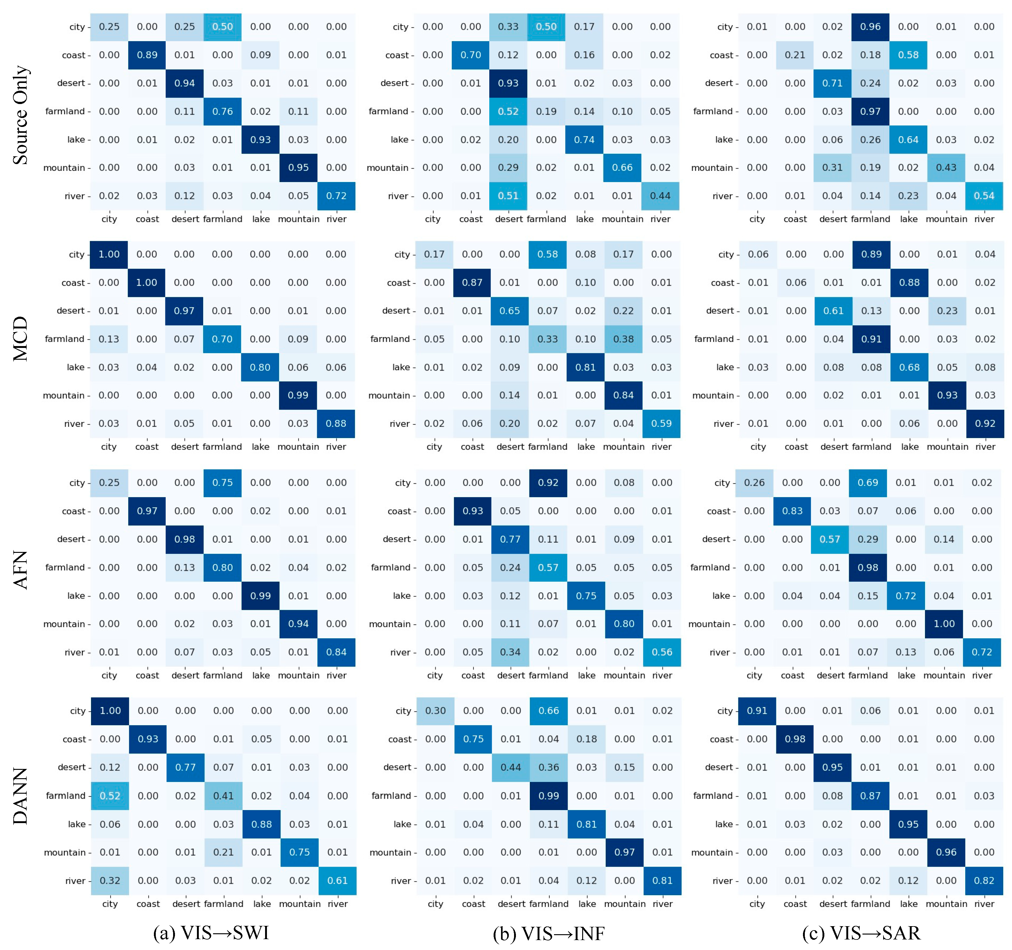
A confusion matrix obtained from the source-only prediction results and the best DA method for three transfer tasks could be used to study the distribution of each class in the experiments.
As shown in Figure 4, in the VIS → SWI task, compared with source only, MCD greatly improved the prediction accuracy of various categories, with only a small amount of misclassification. In the VIS → INF task, the prediction accuracy of source only for most categories was not ideal, and the prediction results of each category improved to a certain extent by using AFN, but city and farmland categories were easily confused. In addition, desert and other categories were also confused. In the VIS → SAR task, the prediction accuracy of DANN was significantly improved compared with source only for most categories, but river was sometimes misclassified as lake.
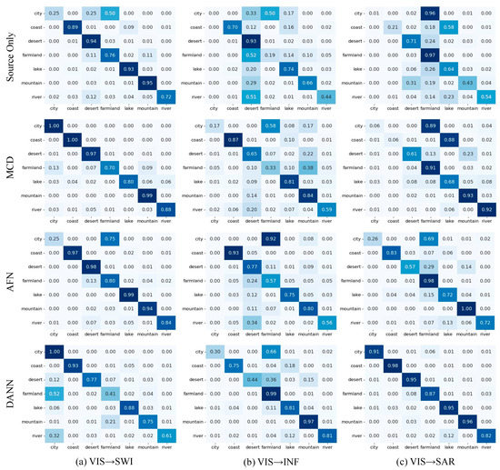
Figure 4.
Confusion matrix of obtained by source-only and DA methods on three tasks.
These experimental results demonstrate the effectiveness of DA, and DA was able to distinguish the appearance difference in different cross-domain tasks. It is a point of follow-up research to study the essence of the performance differences in the different algorithms and design applicable DA algorithms according to the data characteristics.
4.4.3. t-SNE Analysis
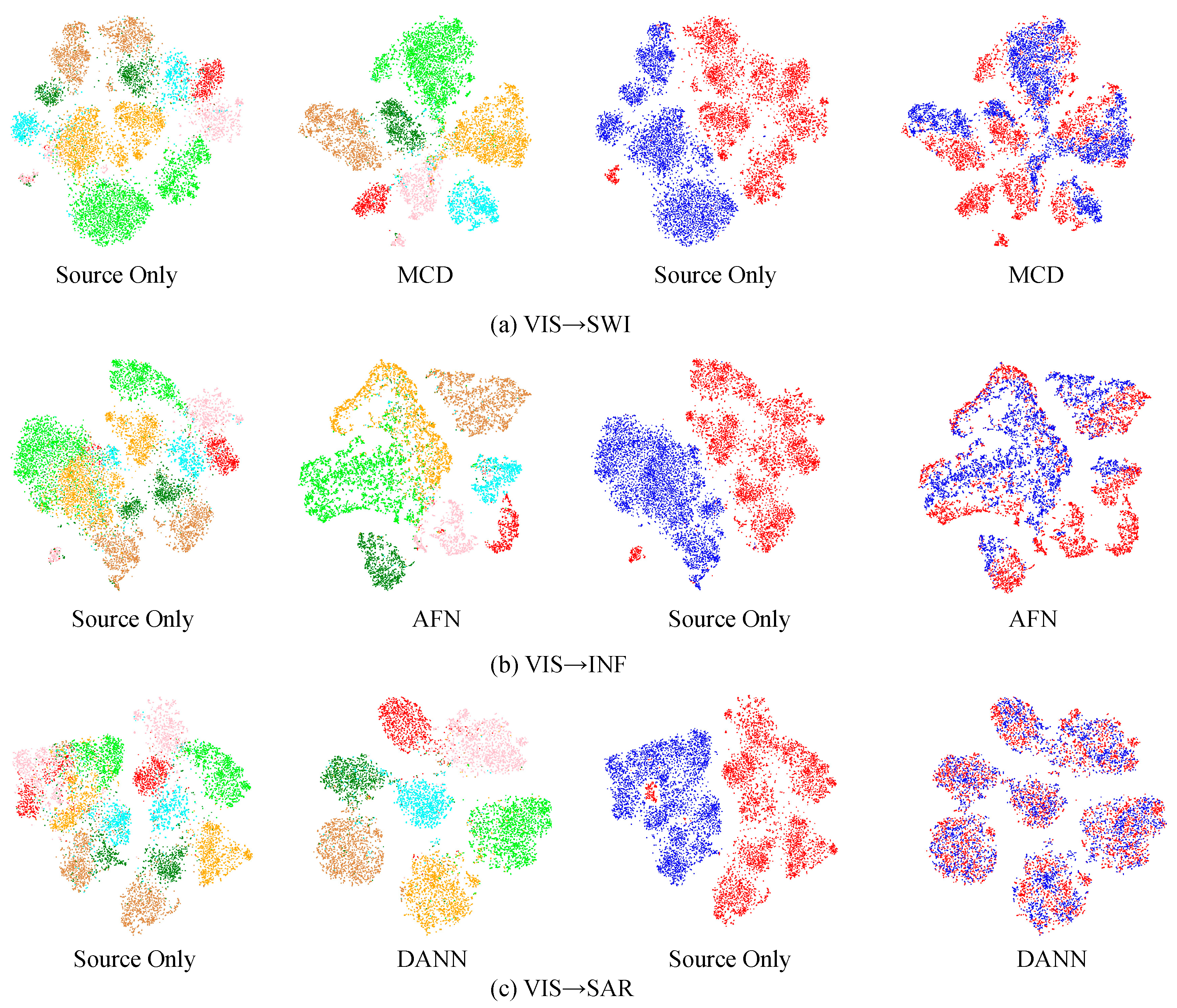
We visualized the features from source only and the best DA method for each task using t-SNE to show the features distributions of the source domain and target domain images extracted by the network. In Figure 5, in the first and second columns, points of each color stands for a category; in the third and fourth columns, points of different colors indicate different domains, where red indicates the source domain and blue indicates the target domain. Odd columns together reflect the corresponding relationship between categories and domains and/or Euclidean columns. The clustering of the same categories means better separability.
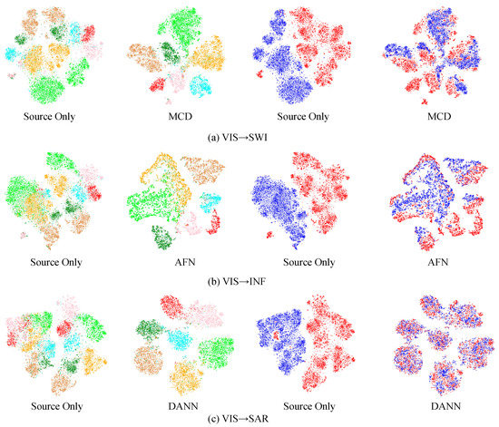
Figure 5.
T-SNE visualizations of the features from distinct DA methods on the (a) VIS → SWI task, (b) VIS → INF task and (c) VIS → SAR task. First and second columns are generated from category information, and each color point indicates a category. Third and fourth columns are generated from domain information; blue points indicate source domain data, and red points indicate target domain data.
The third column of Figure 5 shows that the data from the source domain and target domain are distributed in independent areas, which means that the Resnet-50 network trained only with source domain data cannot align the characteristics of source domain and target domain well. Combined with the category visualization in the first column, it can be seen that the data distribution in the target domain does not form a good category boundary on the (b) VIS → INF task and (c) VIS → SAR task, but the data distribution in the target domain has a boundary on the (a) VIS → SWI task, indicating that the difference between the VIS and SWI data domains is not significant, and the Source Only method can achieve better results in the target domain, which is consistent with the results in Table 3.
As shown in the fourth column of Figure 5, the network trained by the best DA method of the three tasks can align the characteristics of the source domain and the target domain well. Specifically, DANN made separated inter-class and tight intra-class clusters on the (c) VIS → SAR task. However, the effects on the (a) VIS → SWI and (b) VIS → INF tasks are relatively poor, which is related to the imbalance of data categories. The proposed DA methods could not solve this problem better. This visualization shows that the network trained by DA could improve the performance of cross-domain scene classification of three tasks to varying degrees.
4.4.4. Model Interpretability Analysis
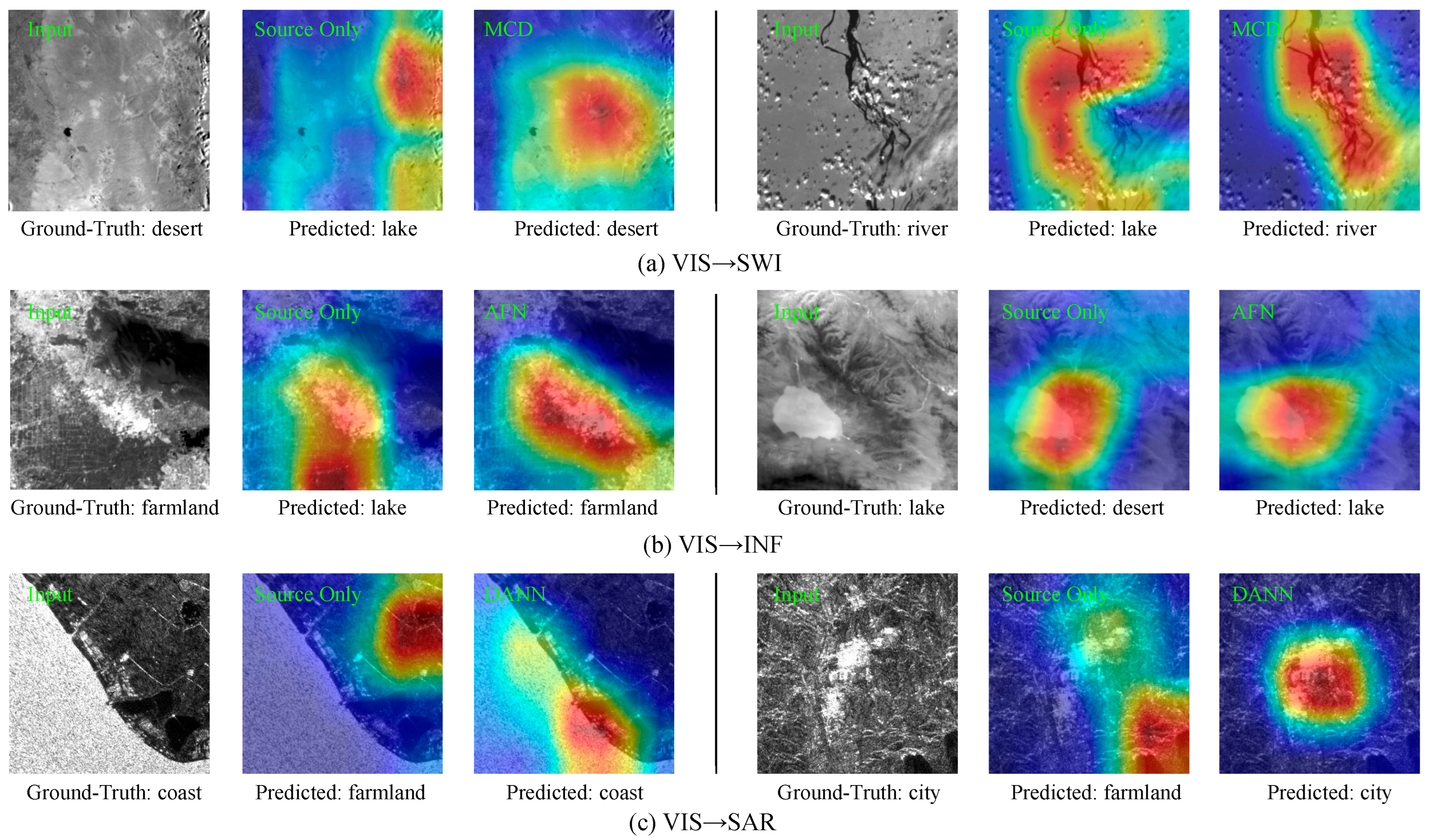
The performance of the DA methods was further analyzed by Grad-CAM visualization. We selected the examples that were easily confused on the three tasks and used the Grad-CAM method to visualize the prediction results of source only and DA. On the generated heatmaps, red indicates that the position prediction category in the graph contributes the most, and blue indicates that the position in the graph contributes the least to the prediction result.
In Figure 6, it can be clearly seen that the source-only method paid attention to the wrong location characteristics, which led to the wrong prediction results. In the case of large domain differences between the training set and the test set, the model-based DA methods could still focus on the correct region and obtain the correct prediction results. Taking the first group of results in Figure 6c as an example, the reason for the incorrect source-only prediction result is that it focused on the land area. However, the semantic label of the input image is coast. Using DA, the model could focus on the location of the coastline and predict correctly, further proving the effectiveness of DA.

Figure 6.
Grad-CAM visualizations of the predicted categories with source only and DA, where (a) VIS → SWI task, (b) VIS → INF task and (c) VIS → SAR task.
5. Discussion of Applications
5.1. Data Annotation
Cross-domain data annotation refers to making full use of the existing labeled datasets and pre-annotating the newly acquired data through domain adaptation.
Currently, many remote-sensing scene classification datasets have been proposed. The data sources, spatial distributions, temporal distributions and classification systems of these datasets have their own characteristics with region differences. Making full use of these marked data to realize the pre-annotation of new data can greatly reduce the annotation cost and improve the automation level of dataset production in remote sensing.
In order to verify the feasibility of DA algorithms in data annotation, we selected five categories, desert, mountain, farmland, river and beach, that are consistent with the MRSSC dataset and the AID dataset for experiments. As shown in Figure 7, the AID dataset was used as the source domain, and the VIS, SAR of the corresponding category in the MRSSC dataset was used as the target domain. We conducted pre-annotation experiment and evaluated them based on the ground truth, finding accuracies of 84.49% and 83.21%. Based on the results of pre-annotation, the labels with low confidence could be modified through manual review, and finally the new data could be constructed.
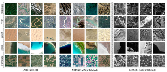
Figure 7.
Example images of cross-domain data annotation.
For the case that the categories of the source domain and the target domain are inconsistent, how to realize the domain adaptation of the same category and reduce the interference of inconsistent categories is a problem worth studying.
5.2. Weakly Supervised Object Detection
A weakly supervised location task uses category information that is weaker than the target task to realize the target location task, that is, to predict the category and location of the target. Weakly supervised target localization based on domain adaptation upgrades the task difficulty. The training set is the sample with category information, and the prediction task is to realize the target localization of samples in different domains from the training set.
Currently, in practical application, the problem encountered by the weak supervised positioning task is that it has achieved good accuracy on the known dataset, but when the algorithm is applied to a new scene, there are domain differences in the data due to different imaging times, imaging locations and even imaging sensors, which will degrade the performance of the model in the new scene. Domain adaptation can solve the problem that the prediction accuracy of the model decreases due to different data distribution and improve the robustness of the model.
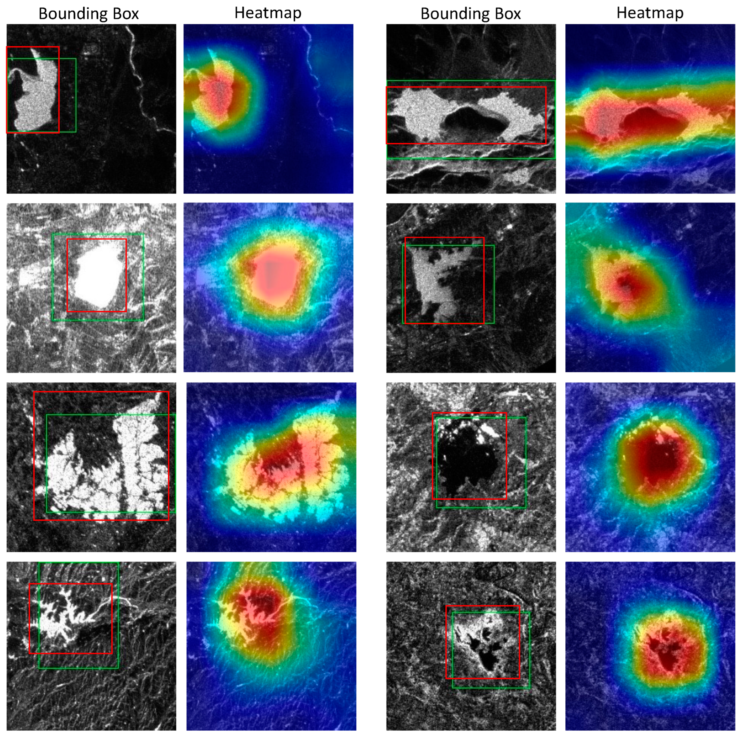
We used MRSSC2.0 to realize the weak supervised location of lakes. The specific experimental setup was as follows: source domain VIS is divided into two types (Lake and non-Lake), and unlabeled SAR is divided into training set and test set by 4:1. Based on DA method, the training sets of source domain VIS and target domain SAR are input into the DA model for training, and the trained model and its parameters are saved. Based on class activation mapping, the thermal map of the output class of the test set is obtained, then the reasonable threshold is set, and the maximum circumscribed rectangle is calculated as the target location result. The experimental results are shown in Figure 8. In each image pair, the left image shows the predicted (green) and ground-truth (red) bounding box. The right image shows the CAM, i.e., where the network is focusing for the object.
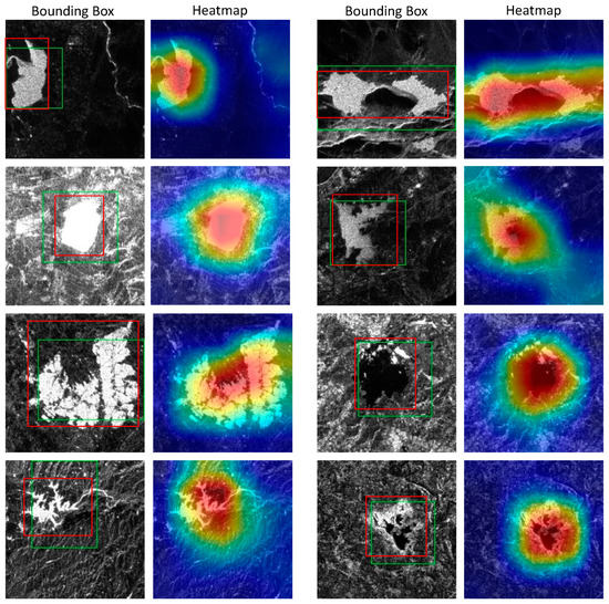
Figure 8.
Qualitative cross-domain weakly supervised lake location results.
The method achieved good weakly supervised location results. This provides a feasible and effective implementation method for in-orbit intelligent real-time remote-sensing image target location, in-orbit service and other application scenarios in different domains of training sets and test sets, and it promotes the development of in-orbit intelligent processing technology.
5.3. Domain Adaptation Data Retrieval
DA methods are also used in data retrieval. For a SAR image, how is it possible to identify the most similar one from a massive optical image dataset? First, based on the scene classification results, the optical images of the same scene were selected. Then we extracted the depth features of the SAR image and the optical image, designed a certain similarity measurement function and took the optical image with the highest similarity as the final result. When there is no rough matching between SAR image and optical image, image registration based on data retrieval can be carried out. Research on the retrieval of optical images and SAR images will be conducive to further fine-grained scene recognition and classification or extended to cross-modal data navigation and positioning.
6. Conclusions
In this paper, we proposed a remote-sensing cross-domain scene classification dataset including four domains and seven scene types. The effectiveness of the domain adaptive methods among VIS, SWI, INF and SAR was verified. Although different domain datasets have great differences, the experimental results show that domain adaptation algorithms can reduce the differences in data distribution between different domains and improve the accuracy of scene classification. However, there are some differences in the mobility between the data of different domains, which are related to the differences in the scale and imaging mechanisms. Improvement can be made for the stability and accuracy of existing DA methods. In addition, addressing unbalanced class distribution and solving the domain adaptation problem of multilabel scene classification tasks still face many challenges. We believe that MRSSC will not only promote the development of cross-domain remote-sensing scene classification but also inspire innovative research on weakly supervised object detection and domain adaptation data retrieval.
Author Contributions
All the authors made significant contributions to the work. Conceptualization, K.L. and S.L.; funding acquisition, S.L.; dataset construction, K.L.; experiment, J.Y.; designed the research and analyzed the results, K.L. and J.Y.; provided advice, S.L. All authors have read and agreed to the published version of the manuscript.
Funding
This work was supported in part by the China Manned Space Science and Applications DataBase at the National Basic Science Data Center under grant NO. NBSDC-DB-17 and in part by the Director′s Foundation of Technology and Engineering Center for Space Utilization, Chinese Academy of Sciences under Grant CSU-JJKT-2020-7.
Data Availability Statement
The datasets proposed in this research are available online. MRSSC2.0 dataset is available for download at http://www.csu.cas.cn/gb/kybm/sjlyzx/gcxx_sjj/sjj_tgxl/202208/t20220831_6507453.html.
Acknowledgments
Thanks to China Manned Space Engineering for providing space science and application data products from Tiangong-2, and thanks for the scientific data from the National Basic Science Data Center China Manned Space Science and Applications DataBase under grant NO. NBSDC-DB-17.
Conflicts of Interest
The authors declare no conflict of interest.
Abbreviations
The following abbreviations are used in this manuscript:
| MRSSC | Multimodal Remote Sensing Scene Classification |
| WIS | Wide-band Imaging Spectrometer |
| InIRA | Interferometric Imaging Radar Altimeter |
| DA | Domain adaptation |
| VIS | Visible Near Infrared |
| SWI | Short Wavelength Infrared |
| INF | Thermal Infrared |
| SAR | Synthetic Aperture Radar |
| OA | Overall accuracy |
| DDC | Deep Domain Confusion |
| MMD | Maximum Mean Discrepancy |
| ADDA | Adversarial Discriminative Domain Adaptation |
| AFN | Adaptive Feature Norm |
| BSP | Batch Spectral Penalization |
| CDAN | Conditional Domain Adversarial Network |
| DAN | Deep Adaptation Network |
| DANN | Domain Adversarial Neural Network |
| JAN | Joint Adaptation Network |
| MCC | Minimum Class Confusion |
| MCD | Maximum Classifier Discrepancy |
| MDD | Margin Disparity Discrepancy |
References
- Cheng, G.; Han, J.; Lu, X. Remote Sensing Image Scene Classification: Benchmark and State of the Art. Proc. IEEE 2017, 105, 1865–1883. [Google Scholar] [CrossRef]
- Xia, G.S.; Hu, J.; Hu, F.; Shi, B.; Bai, X.; Zhong, Y.; Zhang, L.; Lu, X. AID: A Benchmark Data Set for Performance Evaluation of Aerial Scene Classification. IEEE Trans. Geosci. Remote Sens. 2017, 55, 3965–3981. [Google Scholar] [CrossRef]
- Sukhia, K.N.; Riaz, M.M.; Ghafoor, A.; Ali, S.S. Content-Based Remote Sensing Image Retrieval Using Multi-Scale Local Ternary Pattern. Digit. Signal Process. 2020, 104, 102765. [Google Scholar] [CrossRef]
- Huang, W.; Li, G.; Chen, Q.; Ju, M.; Qu, J. CF2PN: A Cross-Scale Feature Fusion Pyramid Network Based Remote Sensing Target Detection. Remote Sens. 2021, 13, 847. [Google Scholar] [CrossRef]
- Chen, Y.; Teng, W.; Li, Z.; Zhu, Q.; Guan, Q. Cross-Domain Scene Classification Based on a Spatial Generalized Neural Architecture Search for High Spatial Resolution Remote Sensing Images. Remote Sens. 2021, 13, 3460. [Google Scholar] [CrossRef]
- Lu, X.; Gong, T.; Zheng, X. Multisource Compensation Network for Remote Sensing Cross-Domain Scene Classification. IEEE Trans. Geosci. Remote Sens. 2020, 58, 2504–2515. [Google Scholar] [CrossRef]
- Liu, K.; Wu, A.; Wan, X.; Li, S. MRSSC: A Benchmark Dataset for Multimodal Remote Sensing Scene Classification. Int. Arch. Photogramm. Remote Sens. Spat. Inf. Sci. 2021, XLIII-B2-2, 785–792. [Google Scholar] [CrossRef]
- Yang, Y.; Newsam, S. Bag-of-Visual-Words and Spatial Extensions for Land-Use Classification. In Proceedings of the 18th SIGSPATIAL International Conference on Advances in Geographic Information Systems, San Jose, CA, USA, 2–5 November 2010; pp. 270–279. [Google Scholar]
- Sumbul, G.; Charfuelan, M.; Demir, B.; Markl, V. Bigearthnet: A Large-Scale Benchmark Archive for Remote Sensing Image Understanding. In Proceedings of the IGARSS 2019-2019 IEEE International Geoscience and Remote Sensing Symposium, Yokohama, Japan, 28 July–2 August 2019; pp. 5901–5904. [Google Scholar] [CrossRef]
- Zhou, Z.; Li, S.; Wu, W.; Guo, W.; Li, X.; Xia, G.; Zhao, Z. NaSC-TG2: Natural Scene Classification with Tiangong-2 Remotely Sensed Imagery. IEEE J. Sel. Top. Appl. Earth Obs. Remote Sens. 2021, 14, 3228–3242. [Google Scholar] [CrossRef]
- Wang, Y.; Zhu, X.X.; Zeisl, B.; Pollefeys, M. Fusing Meter-Resolution 4-D InSAR Point Clouds and Optical Images for Semantic Urban Infrastructure Monitoring. IEEE Trans. Geosci. Remote Sens. 2016, 55, 14–26. [Google Scholar] [CrossRef]
- Wang, L.; Xu, X.; Yu, Y.; Yang, R.; Gui, R.; Xu, Z.; Pu, F. SAR-to-Optical Image Translation Using Supervised Cycle-Consistent Adversarial Networks. IEEE Access 2019, 7, 129136–129149. [Google Scholar] [CrossRef]
- Saenko, K.; Kulis, B.; Fritz, M.; Darrell, T. Adapting Visual Category Models to New Domains. In Proceedings of the European Conference on Computer Vision, Berlin/Heidelberg, Germany, 5–11 September 2010; pp. 213–226. [Google Scholar]
- Peng, X.; Usman, B.; Kaushik, N.; Hoffman, J.; Wang, D.; Saenko, K. Visda: The Visual Domain Adaptation Challenge. arXiv 2017, arXiv:1710.06924. [Google Scholar]
- Tzeng, E.; Hoffman, J.; Zhang, N.; Saenko, K.; Darrell, T. Deep Domain Confusion: Maximizing for Domain Invariance. arXiv 2014, arXiv:1412.3474. [Google Scholar]
- Gretton, A.; Borgwardt, K.; Rasch, M.; Schölkopf, B.; Smola, A. A Kernel Method for the Two-Sample-Problem. Adv. Neural Inf. Process. Syst. 2006, 19, 513–520. [Google Scholar]
- Long, M.; Cao, Y.; Wang, J.; Jordan, M. Learning Transferable Features with Deep Adaptation Networks. In Proceedings of the International Conference on Machine Learning, Lille, France, 6–15 July 2015; pp. 97–105. [Google Scholar]
- Long, M.; Zhu, H.; Wang, J.; Jordan, M.I. Deep Transfer Learning with Joint Adaptation Networks. In Proceedings of the International Conference on Machine Learning, Sydney, Australia, 6–11 August 2017; pp. 2208–2217. [Google Scholar]
- Xu, R.; Li, G.; Yang, J.; Lin, L. Larger Norm More Transferable: An Adaptive Feature Norm Approach for Unsupervised Domain Adaptation. In Proceedings of the IEEE/CVF International Conference on Computer Vision, Seoul, Korea, 27–28 October 2019; pp. 1426–1435. [Google Scholar]
- Jin, Y.; Wang, X.; Long, M.; Wang, J. Minimum Class Confusion for Versatile Domain Adaptation. In Proceedings of the European Conference on Computer Vision, Online, 23–28 August 2020; pp. 464–480. [Google Scholar]
- Ganin, Y.; Ustinova, E.; Ajakan, H.; Germain, P.; Larochelle, H.; Laviolette, F.; Marchand, M.; Lempitsky, V. Domain-Adversarial Training of Neural Networks. Adv. Comput. Vis. Pattern Recognit. 2017, 17, 189–209. [Google Scholar] [CrossRef]
- Long, M.; Cao, Z.; Wang, J.; Jordan, M.I. Conditional Adversarial Domain Adaptation. Adv. Neural Inf. Process. Syst. 2018, 31, 1647–1657. [Google Scholar]
- Saito, K.; Watanabe, K.; Ushiku, Y.; Harada, T. Maximum Classifier Discrepancy for Unsupervised Domain Adaptation. In Proceedings of the IEEE Conference on Computer Vision and Pattern Recognition, Salt Lake City, UT, USA, 18–23 June 2018; pp. 3723–3732. [Google Scholar]
- Chen, X.; Wang, S.; Long, M.; Wang, J. Transferability vs. Discriminability: Batch Spectral Penalization for Adversarial Domain Adaptation. In Proceedings of the International Conference on Machine Learning, Long Beach, CA, USA, 9–15 June 2019; pp. 1081–1090. [Google Scholar]
- Zhang, Y.; Liu, T.; Long, M.; Jordan, M. Bridging Theory and Algorithm for Domain Adaptation. In Proceedings of the International Conference on Machine Learning, Long Beach, CA, USA, 9–15 June 2019; pp. 7404–7413. [Google Scholar]
- Gao, M. Earth Observation Payloads and Data Applications of Tiangong-2 Space Laboratory. In Proceedings of the Tiangong-2 Remote Sensing Application Conference, Singapore, 8 December 2018; pp. 1–13. [Google Scholar]
- Li, S.; Tan, H.; Liu, Z.; Zhou, Z.; Liu, Y.; Zhang, W.; Liu, K.; Qin, B. Mapping High Mountain Lakes Using Space-Borne near-Nadir SAR Observations. Remote Sens. 2018, 10, 1418. [Google Scholar] [CrossRef]
- Der Maaten, L.; Hinton, G. Visualizing Data Using T-SNE. J. Mach. Learn. Res. 2008, 9, 2579–2605. [Google Scholar]
- Selvaraju, R.R.; Cogswell, M.; Das, A.; Vedantam, R.; Parikh, D.; Batra, D. Grad-CAM: Visual Explanations from Deep Networks via Gradient-Based Localization. Int. J. Comput. Vis. 2019, 128, 336–359. [Google Scholar] [CrossRef]
- Zhang, H.; Kyaw, Z.; Chang, S.F.; Chua, T.S. Visual Translation Embedding Network for Visual Relation Detection. In Proceedings of the 30th IEEE Conference Computer Vision and Pattern Recognition, CVPR, Honolulu, HI, USA, 21–26 July 2017; pp. 3107–3115. [Google Scholar] [CrossRef]
- Jiang, J.; Fu, B.; Long, M. Transfer-Learning-Library. 2020. Available online: https://github.com/thuml/Transfer-Learning-Library (accessed on 1 June 2022).
Publisher’s Note: MDPI stays neutral with regard to jurisdictional claims in published maps and institutional affiliations. |
© 2022 by the authors. Licensee MDPI, Basel, Switzerland. This article is an open access article distributed under the terms and conditions of the Creative Commons Attribution (CC BY) license (https://creativecommons.org/licenses/by/4.0/).

