Distinguishing the Impacts of Rapid Urbanization on Ecosystem Service Trade-Offs and Synergies: A Case Study of Shenzhen, China

Abstract

Cities and urban areas are an important part of global sustainable development, and the health and well-being of urban residents are closely related to the quality, quantity, and diversity of urban ecosystem services. Although the rapid urbanization process has changed the structure and function of urban ecosystems, which is notably different from natural ecosystems, the affected ecosystem services and their interactions—the trade-off impact of urbanization intensity on ecosystem services—remain to be discussed. Using land use/land cover and impervious surface area remote sensing datasets, and InVEST and RUSLE-related ecosystem services models to evaluate seven typical ecosystem services in Shenzhen, this study explored the evolution of multiple ecosystem service trade-offs and synergies during the transition from a natural ecosystem to an urban ecosystem, and how they are affected by urbanization intensity through correlation analysis and a discrete time-step simulation model. The results show that: (1) from 1978 to 2018, in the process of ecosystem transformation, grain production dropped from 228,795 tons to 11,733 tons, fruit production peaked in 1990 at 271,508 tons, and service capacity of both showed obvious degradation. Conversely, the cultural service capacity was remarkably enhanced. (2) With the increase in urbanization level, the trade-off and synergy of ecosystem services gradually transition from linear to nonlinear. The rapid urbanization process drives the nonlinear degradation of ecosystem services and the nonlinear enhancement of synergy. (3) Over the past four decades, ecosystem service bundles within the same kilometer grid have shown a quadratic curve-like decrease with increasing impervious surface area, slowly in the early stages and faster in the later stages. This study concludes that urbanization intensity has a significant impact on ecosystem service trade-offs, which can provide support for the formulation of ecological protection and restoration strategies in territorial space based on ecosystem services.

1. Introduction

During the transition from natural ecosystems to urban ecosystems, the structure of the natural ecosystem is fragmented and its function is degraded [1], resulting in insufficient supply capacity of ecosystem services (ESs) and damage to urban resilience, which then evolves into a fragile adaptive urban ecosystem [2]. Urban ecosystem services have certain restrictions on the geographic matching of supply and demand, and the trade-off and synergies of ESs have typical regional characteristics [3]. Revealing the spatial pattern of trade-offs and synergies between ecosystem services under the interaction of human and nature, and then restoring the damaged ecosystem to improve urban resilience, is crucial for urban ecosystem sustainability. The supply of urban ESs depends on the structure and function of multiple systems: social, governance, ecosystems, and the relationships between systems across temporal and spatial scales [4,5]. In urban areas, management measures in social, ecological, or technological dimensions have an impact on the quantity, quality, or spatial and temporal distribution of ES benefits [6], and thus on the trade-offs and synergies of ecosystem services. There is an urgent need to clarify the complex interactions that exist among ESs [7]. Previously, studies on trade-offs and synergies of ESs have focused on productive landscapes, such as the provisioning and regulation of services of agricultural or forest landscapes [8]. There are few studies on urban landscapes that are mainly for human well-being and ecological conservation [9], especially the interaction between urban landscapes and other landscapes [10]. However, mismatches in the spatial scales of supply, delivery, and demand for services can reduce gains and impair the effectiveness of ES management. Ecosystem management decisions cause landscape modification and drive a trade-off between ESs in urban landscapes [11]. Without considering changes in the supply and demand of ESs at different scales [12], it is difficult to ensure that ESs are provided at the time and place required by residents.

The trade-offs and synergies of ES has become a hot topic in urban landscape ecology [11]. Trade-offs can generally be understood and analyzed from three aspects: time, space, and reversibility [7], which are usually highly nonlinear [13,14]. Spatial trade-offs manifest as inverse changes in ESs between regions; in more common terms, an increase in grain production in one region causes a decrease in multiple other services in another region [15]. Temporal trade-offs refer to the negative impacts of changes in ESs in the present on future ecosystems [16]. Reversible trade-offs refer to the balance between reversible and irreversible changes in ESs. However, previous studies have mainly focused on natural ecosystem services and have paid less attention to urban ecosystem services [7,17,18,19,20]. Studies on the trade-offs and synergies of ESs in urban areas mainly focus on spatial identification, characterization variated across spatial and temporal scales, driving mechanisms, and scenario simulation [10]. Among them, most studies identify and determine trade-offs and synergies between different ecosystem services through spatial mapping and statistical analysis [7,21,22,23,24,25]. However, the correlations between different types of ESs have obvious spatial and temporal scale characteristics [7,26]. Differences in spatial scale may create different bundles and spatial distribution of ES supply [27]. At the same time, regional socio-economic development at different stages may correspond to different ES management goals, and the current trade-off management of ecosystem services will inevitably have an impact on the future management strategies of ecosystem services. Currently, most studies are limited to a single temporal and spatial scale, and lack comparative analysis.

Understanding ESs trade-off dynamics, types, and driving mechanisms remains one of the main challenges in urban landscape management [10]. There are two driving forms of trade-off and synergy relationships among ecosystem services: joint drivers and direct interactions [5]. The joint driving factors refer to socioeconomic and ecological factors that collaboratively influence ecosystem services, showing synergistic relationships when both ESs have the same feedback effect on the driving factors and trade-off relationships when the feedback is opposite [28]. Direct interactions are changes in the supply of one ES that directly affect another ES. Bennet et al. [5] proposed a classification based on the driving effect among various ESs to explore the linkages between ESs and their mechanisms. In addition, scenario analysis is also a common method to study the relationship between trade-offs and synergies [10]. Specifically, it refers to analyzing the differences and changes of ESs and their trade-offs and synergies under different scenarios by setting ecological protection or economic development goals [29,30,31]. Previous studies on the relationship of multiple ESs generally used statistical analyses such as correlation, regression, clustering, and redundancy analysis [32], through which they can be summarized into dominant ES bundles [33]. An ESs bundle is a group of ESs with synergistic relationships across space and time [34]. The study of the trade-off and synergy relationships among ESs is the premise of ESs management [7]. Most ES models and decision support tools based on land use and land cover were conducted to estimate the value of ESs and the evolution of ES bundles, such as the InVEST model [35,36]. Remote sensing became a widely used methodology in estimating ESs which provides a variety of datasets across a spatial and temporal extent at a pixel level. Remote sensing not only has the potential to acquire LULC, but also biophysical-based vegetation, climate, and ecosystem features [37]. When coupled with process models, remote sensing could provide a tremendous potential to enhance the assessment of ESs [38].

There is a lack of research on the evolution of ESs affected by rapid urbanization in urban ES studies, especially on trade-offs and synergies during the transformation of natural ecosystems to urban ecosystems. Therefore, the main objective of this study was to explore the dynamic effects of rapid urbanization on ES trade-offs and synergies. We selected representative types of urban ESs, and assessed and analyzed the spatial and temporal evolution of ESs in Shenzhen from 1978–2018, and identified their trade-offs and synergistic relationships to explore the evolutionary characteristics of ESs and their trade-offs in the process of transforming natural ecosystems into urban ecosystems.

2. Materials and Methods

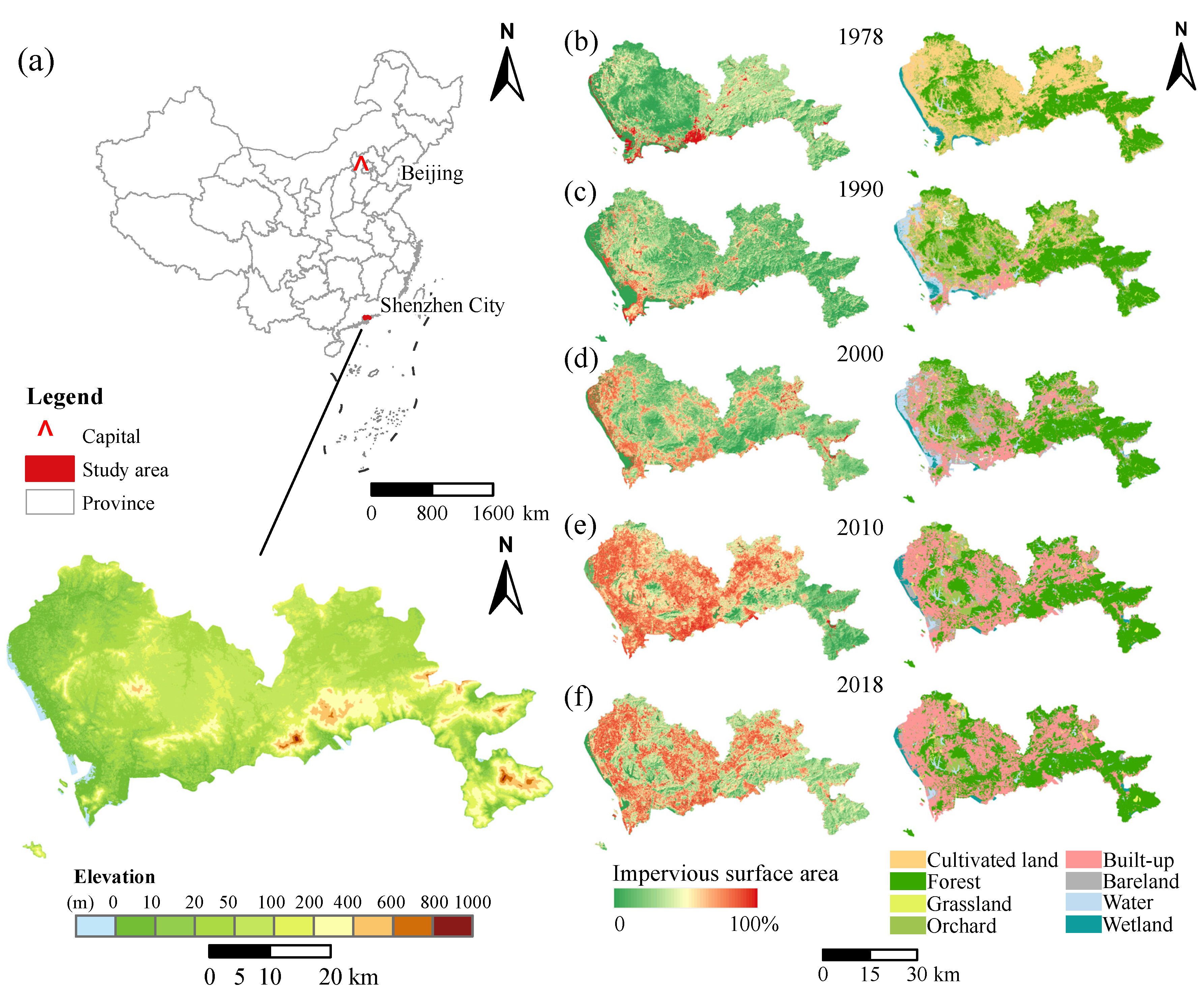
2.1. Study Area

Shenzhen is located in the southeastern part of the Pearl River Delta, with a territorial area of 1997.47 km² and a latitude and longitude range of 113°43′E–114°38′E and 22°24′N–22°52′N (Figure 1). This region has a subtropical monsoon climate with mild temperature and abundant rainfall. The study area does not include Neilingding and other islands in the southwest, which are relatively isolated in the sea. The elevation ranges from zero to 944 m. It is a typical coastal mountainous metropolitan area with ten administrative districts, including four central urban areas (Futian, Nanshan, Luohu, and Yantian) and six suburban areas (Baoan, Guangming, Longhua, Longgang, Pingshan, and Dapeng). After 40 years of development and construction since the reform and opening up, the proportion of cultivated land has shrunk from 45.06% to 1.52%, while the built-up land has expanded from 0.27% to 43.04%. The landscape types and patterns have undergone tremendous changes, which have had a profound impact on the structure, process, and function of the ecosystem. It is a typical area where the evolution and trade-offs of ESs occur.

2.2. Data Sources

The data used in this study mainly include land use/land cover (LULC) data, soil type data, digital elevation model (DEM) data, precipitation and air temperature data, road network data, crop yield data, park data, impervious surface area index, etc. Data descriptions, usage, and sources are shown in

Table 1. Data sources and description.

Type	Description	Usage	Source
Landsat remote sensing images	Landsat 1–3 MSS images of 1978, Landsat 4–5 TM images of 1990, 2000, and 2010, and Landsat 8 OLI-TIRS images of 2018; 30 m resolution	Land use type classification	Geospatial Data Cloud Platform of Computer Network Information Center, Chinese Academy of Sciences(http://www.gscloud.cn, accessed on 12 September 2020)
Land use type	Five years: 1978, 1990, 2000, 2010, and 2018; 30 m resolution	Assessment of multiple ecosystem services	Interpreted from Landsat series remote sensing image data
Precipitation Data	Rainfall in the corresponding year	Calculation of rainfall erosivity and water yield	Shenzhen hydrological statistical yearbook
Temperature data	Average daily temperature for the corresponding year	Calculation of potential evapotranspiration	NOAA (http://www.ncdc.noaa.gov, accessed on 12 September 2020)
Soil type data	Soil type and corresponding soil texture	Assessment of soil retention and water yield	Shenzhen Planning and Land Resources Committee
Road network	Linear vector data	Assessment of Habitat Quality	OpenStreetMap
DEM	Digital elevation model	Watershed and sub-watershed division, slope length and slope factor calculation	Shenzhen Planning and Land Resources Committee
Crop yield	The yield per unit of grain and fruit	Assessment of grain supply and fruit supply	Shenzhen Statistical Yearbook
Parks	Type, boundary, area, and year of opening	Evaluation of park recreation services	Shenzhen City Administration Bureau, Baidu map
Impervious surface area (ISA)	Five years: 1978, 1990, 2000, 2010, and 2018; 30 m resolution	Landscape urbanization level measurement	Interpreted from Landsat series remote sensing image data
Boundary of administrative division	Boundary vector data of each administrative district in Shenzhen; acquired in 2015	Zonal statistics	Shenzhen Planning and Land Resources Committee

.

2.3. Remote Sensing Data Processing

We used temporal Landsat images to produce multi-class land use/land cover maps for 1978, 1990, 2000, 2010, and 2018. In the land use/land cover classification, the decision tree classification (a supervised classification method based on spatial data mining and classification rules) and manual visual interpretation methods were mainly used, which were specifically classified into eight types: cultivated land, forest, grassland, orchard, built-up, bare land, water, and wetland. The impervious surface area data for the corresponding years were obtained through spectral analysis of Landsat images using a combination of the V-I-S model and a linear spectral separation model. The impervious surface index ranged from 0 to 100%. The data accuracy of LULC data and ISA data was generally high to meet the research needs.

2.4. Assessment of ESs

In addition to considering the high intensity of urbanization and human needs in Shenzhen, the urban ecosystem pays more attention to human-centered cultural services than the natural ecosystem. Therefore, this paper adds cultural services on the basis of common ecological service types, and seven types of ecological services were selected, covering four types of services: regulating, supporting, provisioning, and culture. Specifically, habitat quality in supporting services, carbon storage, soil retention, and water yield services in regulating services, grain supply, and fruit supply in provisioning services, and park and recreation services in cultural services.

(1)

Supporting service is mainly calculated as habitat quality (HQ). Using the habitat quality module of the InVEST model, the evaluation result of the model is a dimensionless habitat quality index which ranges from 0 to 1. A higher value indicates better ecological quality and greater capacity to provide supporting services, and vice versa. This module comprehensively evaluates habitat quality based on the quality of the habitat itself (habitat suitability) and the comprehensive threat level to the threat sources (habitat degradation degree), as shown in Equation (1) [39].

$$Q_{xj}=H_j\times \left(1-\left(\frac{D_{xj}^z}{D_{xj}^z+K^Z}\right)\right)$$

(1)

where Q_xj is the habitat quality of grid x in landscape type j, H_j is the habitat suitability of landscape type j, D_xj is the degradation degree of grid x in landscape type j, and K is the half-saturation coefficient. Taking half of the highest degradation degree, z is the model parameter. The formula for calculating the degree of degradation is as follows:

$$D_{xj}={{\displaystyle \sum }}_{r=1}^R{{\displaystyle \sum }}_{y=1}^{Y_r}\left(\frac{W_r}{{{\displaystyle \sum }}_{r=1}^R{W}_r}\right)r_y{i}_{rxy}{\beta }_x{S}_{jr}$$

(2)

$$i_{rxy}=1-\left(\frac{d_{xy}}{d_{rmax}}\right) \mathrm{if} \mathrm{liner}, \mathrm{or}$$

(3)

$$i_{rxy}=exp\left(-\left(\frac{2.99}{d_{rmax}}\right)d_{xy}\right) \mathrm{if} \mathrm{exponential}$$

(4)

where W_r is the weight of threat source r, r_y is the intensity of threat source r, i_rxy is the influence of threat source r in grid x, β_x is the access degree of grid x, S_jr is the sensitivity of landscape type j to threat source r, D_xy is the distance between landscape grid x and threat grid y, and d_rmax is the maximum influence range of threat source r. By referring to similar previous studies [39,40,41,42,43,44], model parameters such as the weight of the threat source, the influence range and habitat suitability, and its sensitivity to the threat factors are set.

(2)

Regulating services are calculated for three ESs: carbon sequestration (CS), water yield (WY), and soil retention (SR). CS and WY are obtained using the carbon module and water yield module of the InVEST model, respectively. In the carbon module, the total carbon storage service is calculated as the sum of the carbon storage of aboveground vegetation, belowground vegetation, dead organic matter, and soil, as shown in Equation (5) [39], and the unit is t/pixel.

$$CS=C_{above}+C_{below}+C_{dead}+C_{soil}$$

(5)

where CS is the total carbon storage, C_above, C_below, C_dead, and C_soil are the carbon storage of aboveground and belowground vegetation, dead organic matter, and soil, respectively. The module is based on land use data and carbon density data, which are mainly based on the results of previous studies on vegetation and soil carbon density [45,46,47,48], of which dead organic matter carbon storage is small and difficult to measure, and is ignored in this study.

In the WY module, water yield (mm) is calculated as the difference between precipitation and actual evapotranspiration based on the water balance principle, as shown in Equation (6) [39].

$$Y\left(x\right)=P\left(x\right)-AET\left(x\right)=\left(1-\frac{AET\left(x\right)}{P\left(x\right)}\right)\times P\left(x\right)$$

(6)

where Y(x) is the annual water yield in grid x, and P(x) and AET(x) are the annual rainfall and the actual evapotranspiration in grid x, respectively. The ratio of them, AET(x)/P(x) is measured by the hydrothermal coupling balance formula proposed based on the Budyko curve, as shown in Equation (7) [49,50].

$$\frac{AET\left(x\right)}{P\left(x\right)}=1+\frac{PET\left(x\right)}{P\left(x\right)}-{\left[1+{(\frac{PET\left(x\right)}{P\left(x\right)})}^{\omega }\right]}^{\frac{1}{\omega }}$$

(7)

where PET(x) is the potential evapotranspiration in grid x and ω refers to the parameter related to climate characteristics and soil properties. Overall, this module uses land use types and their root depth coefficients, annual rainfall, annual potential evapotranspiration, and soil texture data, and adjusts the parameter Z value in combination with the humid climate of Shenzhen.

Soil retention (SR) is calculated according to the revised universal soil loss equation (RUSLE), which is characterized by the soil retention amount, that is, the difference between potential soil erosion and actual soil erosion, as shown in Equation (8), and the unit is t/(hm²·a).

$$A_c=A_p-A_a=R\times K\times LS\times \left(1-C\times P\right)$$

(8)

where A_c is the amount of soil retention and A_p and A_a are the potential and actual soil erosion, respectively. R, K, LS, C, and P represent rainfall erosivity, soil erodibility, slope length and gradient, vegetation coverage, and soil and water retention implementation factors, respectively. This equation adopts rainfall, land use type, and DEM data.

The equation of R is as follow [51]:

$$R_i=\alpha {{\displaystyle \sum }}_{j=1}^k{\left(D_j\right)}^{\beta }$$

(9)

$$\alpha =21.586{\beta }^{-7.1891}$$

(10)

$$\beta =18.144P_{d12}^{-1}+24.225P_{y12}^{-1}+0.8363$$

(11)

where R_i is the ith half month rainfall erosion, k is the days of the precipitation over 12 mm per time in ith half month, D_j is the erosive rainfall of the jth day in half month period in which the daily rainfall less than 12 mm is 0, and α and ꞵ are the model parameters. These values are references in a local scale.

The LS can be acquired from the following equation [52]:

$$L={\left(\frac{l}{22.13}\right)}^a$$

(12)

$$S=\{\begin{array}{c}10.8sin\theta +0.03 \theta < 9\%\\ 16.8sin\theta -0.50 \theta \ge 9\% \end{array}$$

(13)

where L is the slope length factor (m), a is a parameter controlled by the value of the slope. Slope over 5%, a is equal to 0.5; Slope between 3–5%, a is equal to 0.4; Slope below 3%, a is equal to 0.3. S is the slope factor and θ is the slope (%).

C and P are the inhibition factors of soil erosion and their values range from 0 to 1. The smaller their values are, the greater their inhibition effect on soil erosion is. In this study, C and P are mainly characterized by land use/land cover types. Based on previous studies [39], we adjust the C and p values according to Shenzhen’s land use/land cover types (

Table 2. The C and P values in different LULC of Shenzhen.

LULC	Cropland	Orchard	Forest	Built-Up	Water	Bare Land	Wetland	Grassland
C	0.38	0.18	0.004	0	0	1	0	1
P	0.02	0.4	1	1	0	1	1	1

).

In addition, the parameter K is shown in

Table 3. K value based on the soil type map (Unit: t•hm²•h•hm⁻²•MJ⁻¹•mm⁻¹).

Soil Type	K Value
Coastal sandy field/mudflat soil	0.134
Lateritic red soil	0.191
Sand shale yellow soil	0.205
Yellow mud soil	0.209
Granite yellow soil	0.221
Granite red soil	0.232
Red mud soil	0.250
Black mud field/Chisley soil/Vegetable field	0.268
Sand shale lateritic soil	0.277
Alluvial soil/Tidal sand soil/Delta sedimentary soil	0.284
Sand shale red soil	0.291
Eroding red soil	0.292
Saline soil/Acid sulfate paddy soil	0.295
Marsh soil	0.303

.

(3)

Provisioning services are calculated for two kinds of production supply: grain production (GP) and fruit production (FP). The grain and fruit production data provided by the Shenzhen Statistical Yearbook, as well as the area of cropland and orchard land in the corresponding years, are used to spatially quantify the grain and fruit supply services at the grid scale in Shenzhen. The following formulas were used to allocate the GP and FP into pixel values:

$$L_i=C_i\times P_L$$

(14)

$$S_i=O_i\times P_S$$

(15)

where L_i is the grain production in pixel i, S_i is the fruit production in pixel i, C_i and O_i are the area of the cropland and orchard in the pixel i, and P_L and P_S are the grain yield and fruit yield, respectively.

(4)

Park and recreation services (PR) are considered for cultural services. Parks are important recreational places for urban residents and can provide a variety of cultural services. Shenzhen has a complete park classification system and a large number of parks. The cultural service is represented by the park recreation service, and its value is determined by the coverage times of service scope and the service capacity of the park [53,54,55]. Four indicators, park area, type, naturalness, and water coverage, are selected to comprehensively evaluate park and recreation services. The weights of each indicator are obtained by the entropy weight method and are 0.32, 0.08, 0.09 and 0.51, respectively. Therefore, the calculation formula of park service capacity is as follows:

$$P=0.32AR+0.08TY+0.09NA+0.51WB$$

(16)

In the formula, P stands for the park service capacity and AR, TY, NA, and WB are the indicators of park area, type, naturalness, and water coverage selected in this study, respectively. Finally, according to the service radius of the park, the service capacity index of all parks in Shenzhen each year is summed up and counted to obtain the spatial distribution of park recreation services [56].

2.5. Analysis of ES Trade-Off and Synergy Relationships

Based on a kilometer grid scale, Shenzhen was divided into 2208 grids of 1 km × 1 km, the standardized ES data was counted into each grid, and correlation analysis was performed on 2208 samples. First, to eliminate unit and dimensional differences among ESs, the data were normalized using the min–max standardization method, and the formula was as follows:

$$X^{*}=\frac{X-X_{min}}{X_{max}-X_{min}}$$

(17)

where X is the original value of a certain ES, X_min and X_max are the minimum and maximum values of the ES type, respectively, and X* is the standardized value of the ES.

After validation, all the standardized data were in line with normal distribution. Then, Pearson correlation analysis and t-test were used to determine the trade-off and synergy relationships among seven ESs using the correlation coefficient and significance test. A pair of ESs with r ≥ 0.1 and p < 0.01 is defined as a synergy relationship, and the larger r is, the stronger the synergy relationship is. When r ≤ −0.1 and p < 0.01, it is a trade-off relationship, and the smaller r is, the stronger the trade-off relationship is. Otherwise, there is no synergy or trade-off relationship. In addition, using the pairwise ES scatter plot and multiple regression curve, the trade-off and synergy evolution of the ES are analyzed.

Moreover, the ES types were aggregated into seven clusters, corresponding to seven ES bundles (ESB) using a K-means unsupervised clustering method [57] in R statistical software [58]. The ESB value of average standard ES data were used to represent the quantitative value of trade-off and synergy in a 1 km × 1 km gird.

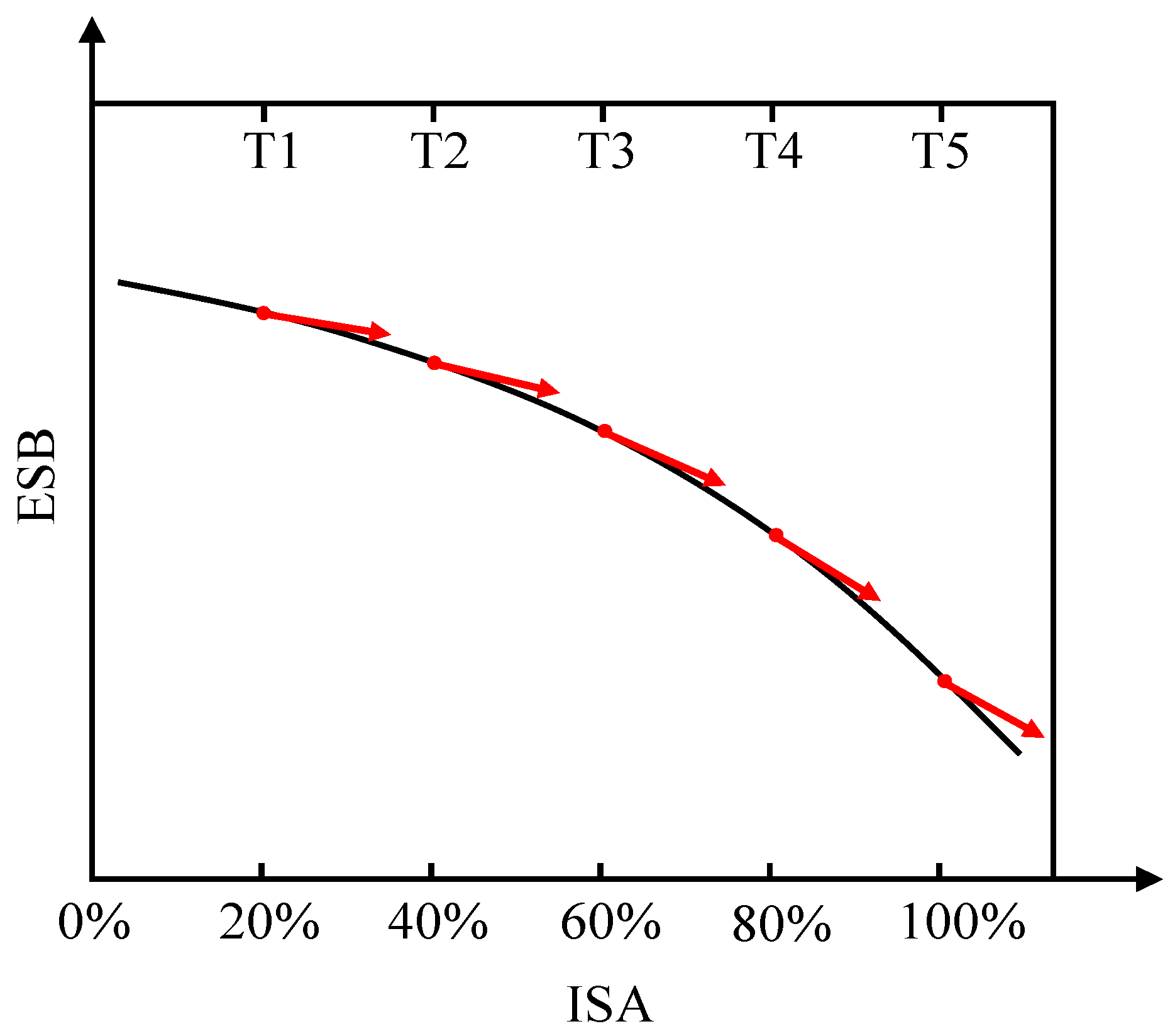
2.6. Relationship between ESB and Urbanization

In order to quantify the dynamic change of the relationship between trade-off and synergy of ESB associated with the urbanization, the discrete time-step simulation model was introduced to fit the ESB and urbanization level represented by ISA at different stages. The level of urbanization evolved from ISA < 20% to ISA > 80% at each period from T₁ to T₅ in a 1 km × 1 km grid, and was used as the sampling method in the model. Thus, we were able to use a theoretical model to describe these relationships of ESs along with the rapid urbanization process. The theoretical curve is shown in Figure 2, which consist of many grids values. Taking the fixed grid change over time as the sample size, a relationship was established to describe the impact of urbanization on ES trade-off and synergy.

The fitting curve formula is as follows:

$$ES{B}_i=aIS{A}_i^2+b IS{A}_i+c$$

(18)

where ESB_i is the standardized mean of the ES bundles, ISA_i is the impervious surface area index, i is the year, and a, b, and c are the model parameters. Shenzhen is divided into 2208 grids of 1 km × 1 km.

3. Results

3.1. Spatial and Temporal Variation of ESs

Since 1978, Shenzhen has developed from a traditional agricultural county into a highly urbanized metropolis. During the transition from the former natural ecosystem dominated by agriculture to the current urban ecosystem with high-intensity urbanization, ESs underwent dramatic changes. The evolution characteristics of seven ESs indicate that ecosystem supporting services were severely degraded, regulating services increased in a fluctuating manner, provisioning services tended to disappear, and cultural services were significantly enhanced (Figure A1).

Specifically, the HQ in Shenzhen was severely degraded and the ecological environment quality became significantly worse from 1978–2018 (Figure 3a). The area with low habitat quality increased by 46%, while the area with high habitat quality decreased from 39% to 17%. The spatial distribution was very uneven, and the high habitat quality was maintained mainly in the eastern area of Shenzhen. The spatial and temporal changes of HQ showed degradation characteristics at different stages of urban development.

The CS in the regulating service was in the range of ~11.15–12.35 million tons, showing an overall trend of continuous decline followed by a rebound, and the spatial distribution shows a pattern of higher carbon storage in the east and lower carbon storage in the west (Figure 3b). In terms of SR, the average annual soil erosion was about 4 million tons, 67% of which was caused by areas of intense erosion, and most of the remaining areas had low soil erosion intensity, with an average of 94% of the areas below moderate erosion, showing an overall distribution pattern of high in the east and low in the west. The potential erosion was much larger than the actual erosion, so the soil retention was close to the potential erosion, and the annual average soil retention was 121.21 million tons. Areas with high soil retention were basically consistent with forest distribution (Figure 3c). WY was profoundly affected by the size and distribution of rainfall, and the overall distribution pattern gradually decreased from east to west. Their total fluctuated greatly between years, with an annual water yield of 3.95 × 10⁹ m³ in 2018 (Figure 3d).

GP is determined by the area of cropland and the yield of grain. However, cropland is the landscape type that has changed most dramatically in Shenzhen over the past 40 years, declining from 45% to 1.5% of the land area, which led to a decrease in GP from 228,795 tons to 11,733 tons (Figure 3e). FP peaked in 1990 with 271,508 tons, and then declined significantly with the decline of orchard area and fruit yield. In 2018, there was considerable fruit production with 46,476 tons, but its orchard area was the lowest in past years and was more limited and concentrated in spatial distribution range (Figure 3f).

Cultural services were the only service type that has been continuously enhanced. The PR has been significantly enhanced in a large area during the past 40 years, but it has always been showing an obviously unbalanced distribution in space with the central city significantly higher than the suburbs, while the high-value center of cultural services in Shenzhen gradually shifted from Luohu to Futian after 2000 (Figure 3g).

By comparing the ESs in 2018 and 1978 (Figure 3a–h), it can be seen that in the process of transformation from natural ecosystem to urban ecosystem, provisioning services were the most obvious service type in decline, showing basically decline to loss by 2018. In addition, supporting services have also degraded significantly, the habitat quality has declined year by year, the area of decline was extensive, and the spatial distribution was highly consistent with the urban construction and development area. Cultural services were the only ESs that were enhanced year by year. In regard to regulating services, carbon storage was relatively stable, the soil retention mainly changed in a small range, and water yield service was affected by the interannual change of rainfall with obvious temporal and spatial fluctuations.

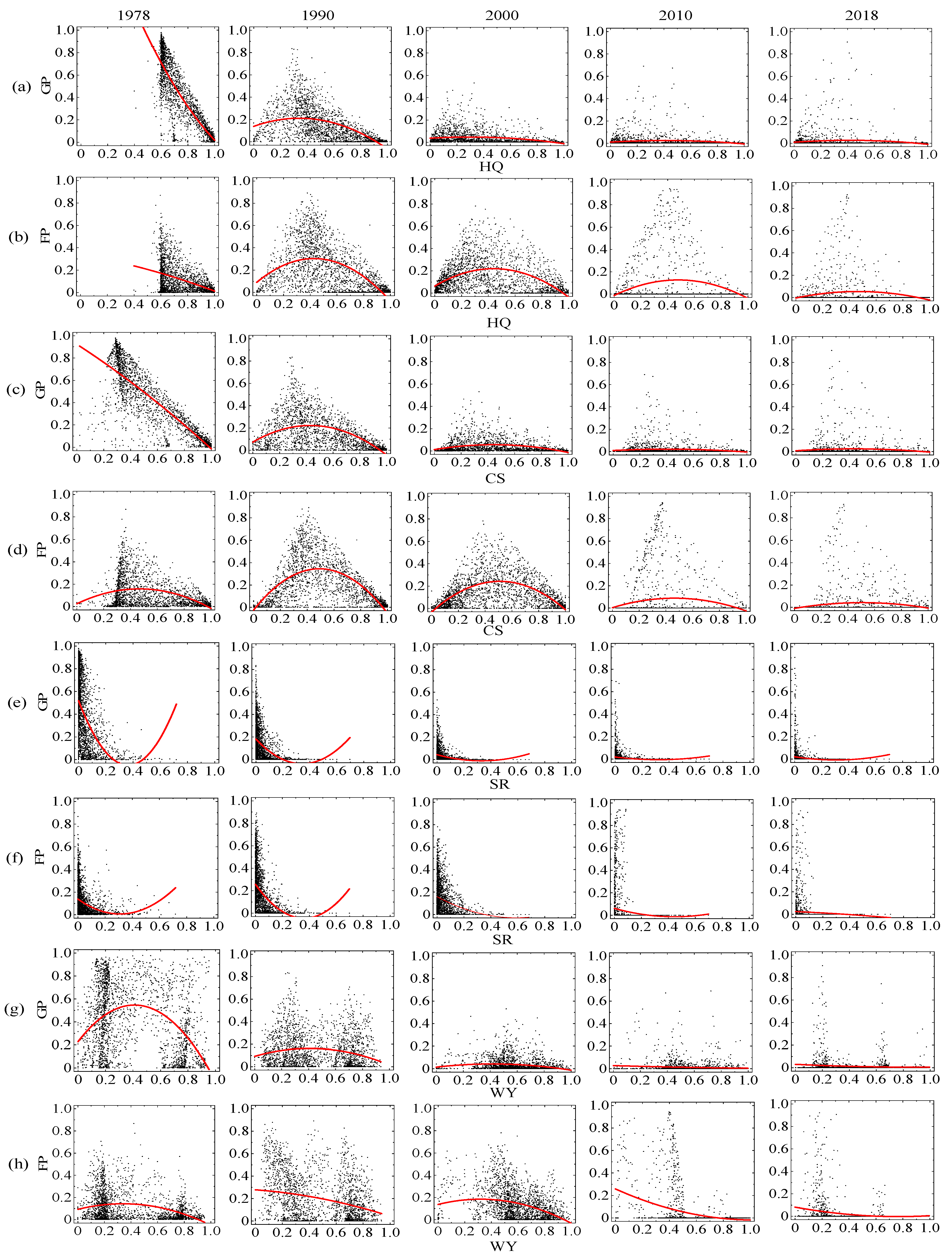
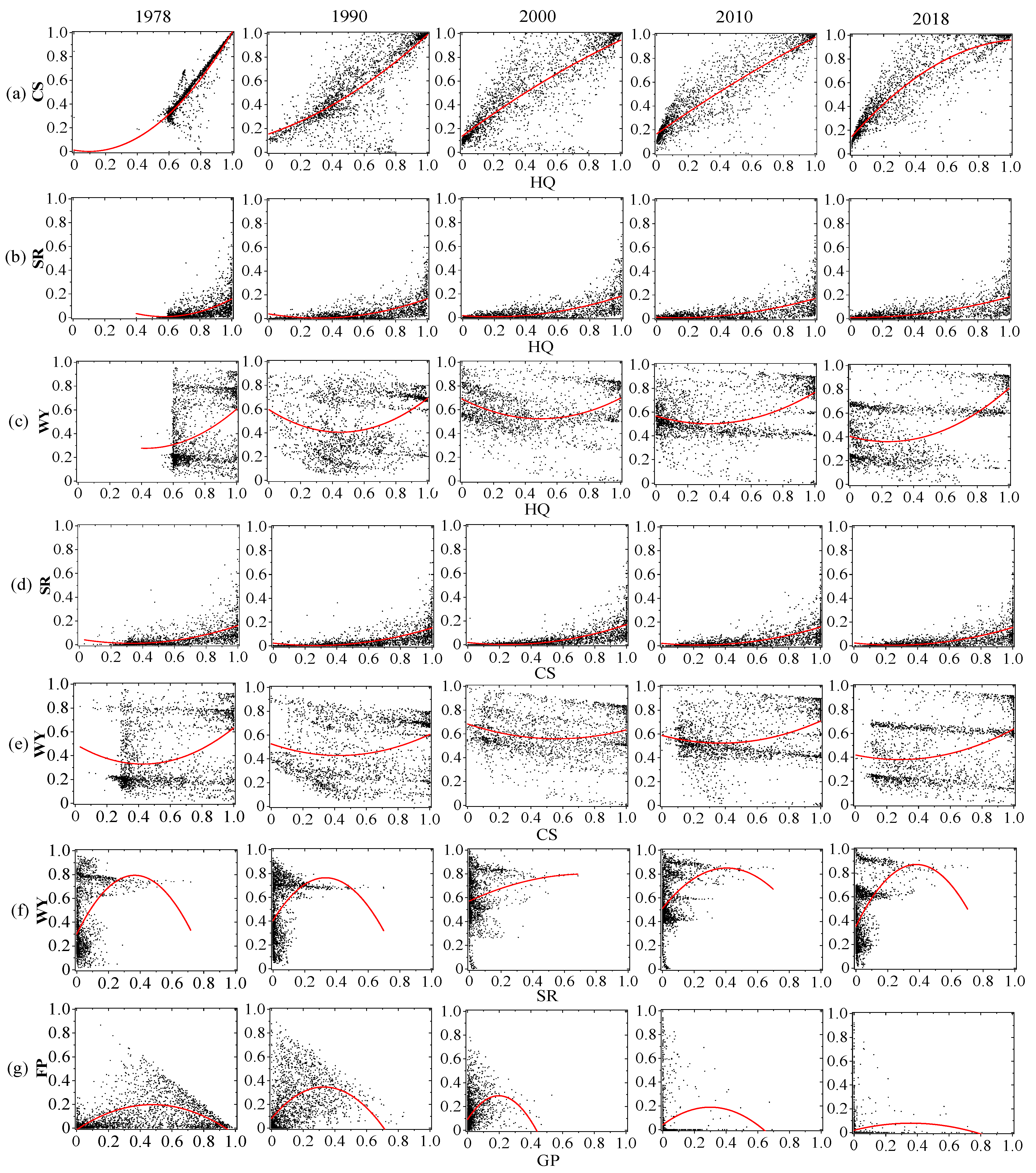
3.2. Evolution of ES Trade-Offs and Synergies

Using Pearson correlation analysis, the results show the trade-offs and synergy relationships among ESs in Shenzhen (Figure 4). Among the 21 pairs of ES matrixes consisting of seven ESs, 9 pairs (HQ–CS, HQ–SR, CS–GP, SR–GP, WY–GP, WY–FP, FP–PR, CS–SR, and SR–WY) consistently maintained significant trade-off or synergy relationships during 1978 to 2018, and 18 pairs showed significant trade-off or synergy relationships in the three or more stages. Within these relationships, ES combinations are quite different.

In general, the trade-offs and synergies of ESs have changed significantly with the process of urbanization. During the transition from natura agricultural ecosystems in 1978 to urban natural ecosystems in 2018, only the mutually reinforcing relationship of strong synergy between regulating and supporting services remained unchanged. However, the relationship among regulating services and between provisioning and regulating services shifted from a strong to a weak trade-off, cultural services and provisioning services improved from a weak to a strong synergy, and cultural services and regulating services changed from a weak to a strong synergy as well.

The main types of ES pairs with trade-offs were: supporting services and provisioning services (including HQ and GP, HQ and FP), regulating services and provisioning services (including CS and GP, CS and FP, SR and GP, SR and FP, WY and GP, and WY and FP) (Figure 5). The fitted curve equations of the trade-off ESs are shown in

Table A1. Equations of fitted curves for ecosystem services pairs with trade-offs.

Ecosystem Services Pairs	Equation; R-Squared Value
	1978	1990	2000	2010	2018
GP-HQ	y = 1.137x2 − 3.549x + 2.429; R2 = 0.729	y = −0.633x2 + 0.431x + 0.139; R2 = 0.340	y = −0.120x2 + 0.070x + 0.037; R2 = 0.101	y = −0.087x2 + 0.071x + 0.010; R2 = 0.032	y = −0.103x2 + 0.085x + 0.009; R2 = 0.020
FP-HQ	y = −0.121x2 − 0.205x + 0.339; R2 = 0.187	y = −1.167x2 + 0.997x + 0.090; R2 = 0.353	y = −0.811x2 + 0.713x + 0.063; R2 = 0.266	y = −0.610x2 + 0.583x − 0.013; R2 = 0.117	y = −0.269x2 + 0.250x − 0.004; R2 = 0.353
GP-CS	y = −0.258x2 − 0.779x + 0.923; R2 = 0.712	y = −0.811x2 + 0.695x + 0.073; R2 = 0.345	y = −0.224x2 + 0.199x + 0.012; R2 = 0.142	y = −0.072x2 + 0.058x + 0.010; R2 = 0.030	y = −0.090x2 + 0.077x + 0.007; R2 = 0.021
FP-CS	y = −0.610x2 + 0.569x + 0.026; R2 = 0.193	y = −1.535x2 + 1.506x − 0.024; R2 = 0.460	y = −1.058x2 + 1.078x − 0.032; R2 = 0.386	y = −0.396x2 + 0.367x + 0.003; R2 = 0.054	y = −0.200x2 + 0.202x − 0.010; R2 = 0.028
GP-SR	y = 4.288x2 − 3.121x + 0.519; R2 = 0.242	y = 1.858x2 − 1.277x + 0.181; R2 = 0.147	y = 0.501x2 − 0.332x + 0.044; R2 = 0.066	y = 0.233x2 − 0.149x + 0.019; R2 = 0.018	y = 0.308x2 − 0.188x + 0.021; R2 = 0.014
FP-SR	y = 1.376x2 − 0.849x + 0.138; R2 = 0.078	y = 2.308x2 − 1.667x + 0.257; R2 = 0.147	y = 0.548x2 − 0.641x + 0.159; R2 = 0.072	y = 0.375x2 − 0.334x + 0.062; R2 = 0.012	y = −0.034x2 − 0.054x + 0.025; R2 = 0.002
GP-WY	y = −0.269x2 + 0.250x − 0.004; R2 = 0.353	y = −0.423x2 + 0.345x + 0.093; R2 = 0.024	y = −0.090x2 + 0.077x + 0.007; R2 = 0.021	y = 0.008x2 − 0.031x + 0.029; R2 = 0.008	y = 0.031x2 − 0.056x + 0.031; R2 = 0.010
FP-WY	y = −0.444x2 + 0.301x + 0.093; R2 = 0.084	y = −0.147x2 − 0.088x + 0.279; R2 = 0.078	y = −0.469x2 + 0.298x + 0.138; R2 = 0.112	y = 0.263x2 − 0.538x + 0.258; R2 = 0.122	y = 0.143x2 − 0.220x + 0.082; R2 = 0.053

.

During the process of transition from a natural ecosystem to an urban ecosystem in Shenzhen, the trade-off status between supporting services and provisioning services gradually changed from a linear to a nonlinear relationship. Among them, HQ and GP had a trade-off relationship from 1978 to 2000, but the Pearson correlation coefficient changed from −0.863 to −0.284, which means the trade-off intensity gradually decreased and was not significant after 2010. In 1978, the trade-off between HQ and GP was linear, and the fit changed to a nonlinear curve after 1990 (Figure 5a). HQ and FP were also in a trade-off relationship from 1978 to 2000, and showed a trend of first increasing and then decreasing and was insignificant from 2000 to 2018 (Figure 5b).

There was also a general trade-off between regulating services (CS, SR and WY) and provisioning services (GP and FP), but the trade-off tended to weaken along with gradual loss in provisioning services (Figure 5c,d). Among them, the trade-off between CS and provisioning services was mainly due to the reduction in cropland and orchard land for supporting services through encroaching on forests in the early stage, resulting in a decrease in carbon density and carbon storage. SR and supporting services had a certain trade-off relationship, showing a U-shaped from 1978 to 1990, and most of the trade-off pairs are distributed on the left side of the U-shaped line, indicating that the supporting services in most areas decreased with the increase in soil retention. Their trade-off relationship has been weakening since 1990 (Figure 5e,f). The trade-off between WY and supporting services was the weakest, and the water yield was greatly influenced by the magnitude and distribution of precipitation (Figure 5g,h).

Supporting services and regulating services (including HQ and CS, HQ and SR, HQ and WY), three types of regulating services (including CS and SR, CS and WY, SR and WY), and two types of provisioning services (GP and FP) were the main synergistic ES pairs (Figure 6). The fitted curve equations of the synergy ESs are shown in

Table A2. Equations of fitted curves for ecosystem services pairs with synergies.

Ecosystem Services Pairs	Equation; R-Squared Value
	1978	1990	2000	2010	2018
CS-HQ	y = 1.230x2 − 0.232x + 0.013; R2 = 0.915	y = 0.380x2 + 0.456x + 0.155; R2 = 0.641	y = −0.181x2 + 0.990x + 0.136; R2 = 0.703	y = −0.128x2 + 0.940x + 0.166; R2 = 0.844	y = −0.695x2 + 1.505x + 0.149; R2 = 0.855
SR-HQ	y = 0.830x2 − 0.956x + 0.284; R2 = 0.386	y = 0.349x2 − 0.220x + 0.040; R2 = 0.428	y = 0.265x2 − 0.101x + 0.017; R2 = 0.470	y = 0.212x2 − 0.054x + 0.012; R2 = 0.460	y = 0.191x2 − 0.018x + 0.011; R2 = 0.476
WY-HQ	y = 0.998x2 − 0.847x + 0.456; R2 = 0.150	y = 0.942x2 − 0.847x + 0.596; R2 = 0.136	y = 0.682x2 − 0.676x + 0.692; R2 = 0.092	y = 0.591x2 − 0.392x + 0.567; R2 = 0.172	y = 0.772x2 − 0.367x + 0.403; R2 = 0.303
SR-CS	y = 0.333x2 − 0.220x + 0.048; R2 = 0.384	y = 0.277x2 − 0.148x + 0.023; R2 = 0.422	y = 0.292x2 − 0.141x + 0.018; R2 = 0.491	y = 0.260x2 − 0.122x + 0.021; R2 = 0.441	y = 0.271x2 − 0.140x + 0.023; R2 = 0.441
WY-CS	y = 0.925x2 − 0.790x + 0.497; R2 = 0.138	y = 0.541x2 − 0.461x + 0.526; R2 = 0.060	y = 0.392x2 − 0.442x + 0.684; R2 = 0.030	y = 0.470x2 − 0.349x + 0.588; R2 = 0.104	y = 0.496x2 − 0.279x + 0.419; R2 = 0.138
WY-SR	y = −3.710x2 + 2.707x + 0.300; R2 = 0.227	y = −3.302x2 + 2.184x + 0.403; R2 = 0.160	y = −0.414x2 + 0.614x + 0.572; R2 = 0.046	y = −2.069x2 + 1.675x + 0.512; R2 = 0.181	y = −3.598x2 + 2.733x + 0.353; R2 = 0.274
FP-GP	y = −0.928x2 + 0.884x − 0.012; R2 = 0.280	y = −2.420x2 + 1.600x + 0.082; R2 = 0.244	y = −5.125x2 + 2.016x + 0.092; R2 = 0.170	y = −1.659x2 + 0.991x + 0.041; R2 = 0.023	y = −0.463x2 + 0.331x + 0.020; R2 = 0.008

. HQ had the strongest synergy relationship with CS over the 40 years, and the correlation coefficients ranged from 0.796 to 0.967 (Figure 6a). There was also a strong synergy between HQ and SR, with a correlation coefficient of 0.581–0.662 (Figure 6b). The synergy relationship between HQ and WY was relatively weak, fluctuated greatly, and showed a non-significant correlation in 2000 (Figure 6c). In addition, the correlation coefficient between CS and SR was always greater than 0.59, indicating strong synergy (Figure 6d). CS and WY showed a weak synergy (Figure 6e). SR and WY showed a moderate synergy (Figure 6f). GP and FP had a weak synergy relationship in provisioning services, which first increased and then continued to weaken between 1978 and 2010. By 2018, the synergy was not significant (Figure 6g).

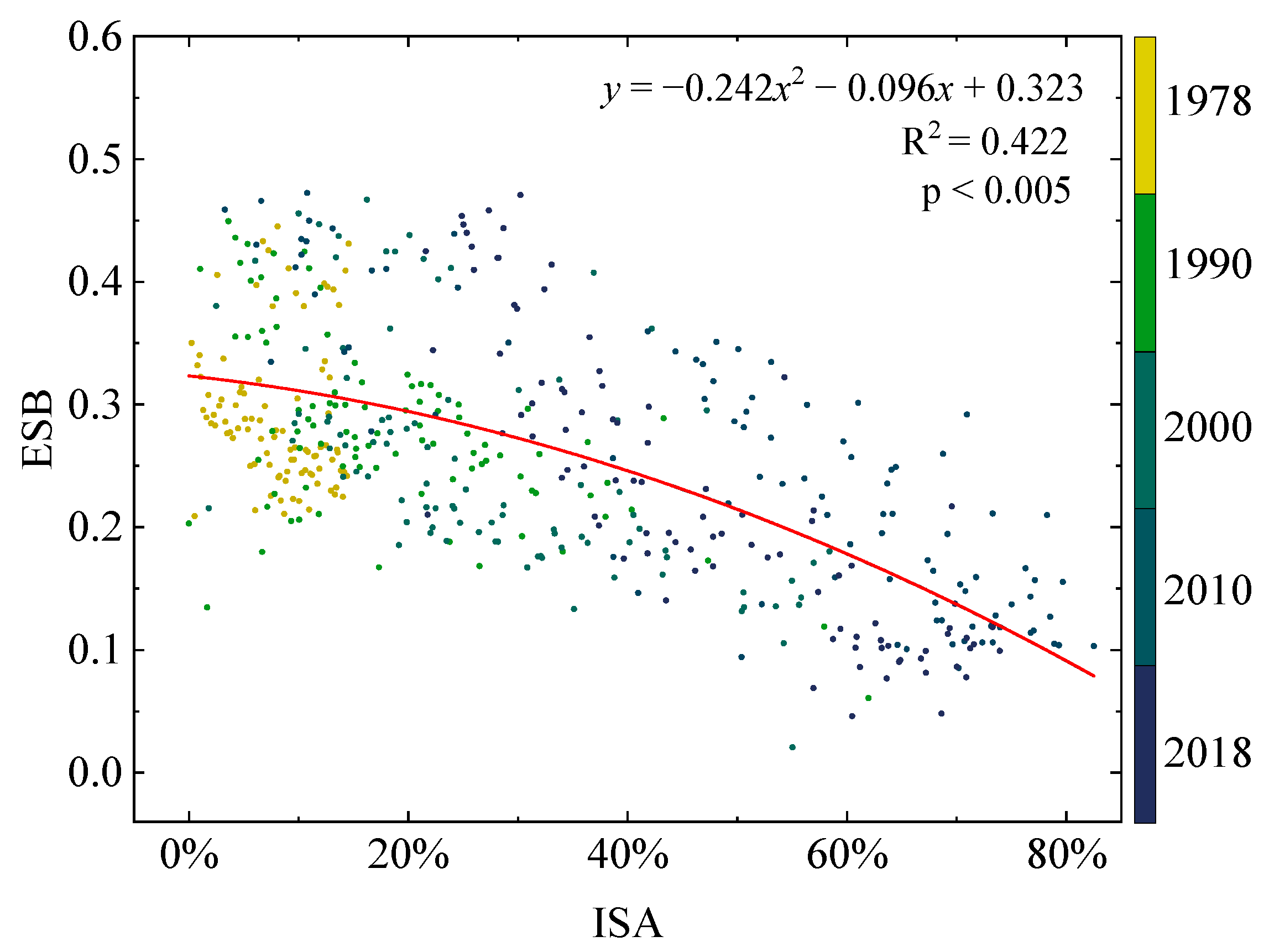
3.3. The Impact of Urbanization Intensity on ES Trade-Off and Synergy

The rapid urbanization process has significantly changed the evolution characteristics of ESs, manifesting as a significant negative impact in space and an S-shaped curve evolution relationship in time. The nonlinear characteristics between the trade-offs of ESs are significantly weakened, and the nonlinear synergies among ESs are significantly enhanced.

We sampled the grid with a value of ISA < 20% in 1978 initially and an increase in ISA occurring over four successive periods. It contains 75 sampling grids accounting for 3.4% of total grids in Shenzhen, and a total number of 375 datasets in five stages has been used to establish the relationship between ISA and ES bundles values at a 1km grid scale to quantify the impacts of urbanization intensity impacts on ES bundles change. Hence, a significant quadratic curve function relationship is found between the two over time, with a fitted equation of ESB = −0.242ISA² − 0.096ISA + 0.323 (R² = 0.422, p < 0.005), and the fitted curve (Figure 7) has a good coincidence with the theoretical curve (Figure 2). The results indicate that the trade-off and synergy relationship of ESs decreases nonlinearly with the increase in ISA, which is slow in the initial stage and fast in the later stage. This nonlinear evolution, influenced by rapid urbanization, strengthens the synergy effect of ESs, while weakening the trade-off effect of ESs.

4. Discussion

4.1. Urbanization Influence on ESs Relationship

This study quantifies the impact and response of urbanization on ESs change. In rapidly urbanizing areas, the structure and types of ecosystems have changed significantly with the process of urbanization, which has led to an increased demand for ESs and decreased supply of ESs [59,60]. However, the responses of changes in ES types are inconsistent, with some services continuing to decline, some services continuing to increase, and some services fluctuating and changing during the process of rapid urbanization. During these changes, the trade-offs and synergies of ES types have also undergone a significant transformation process.

Both urban ESs and natural ESs are subject to decline under the influence of urban expansion and human activities during urbanization. There is a general synergy between supporting and regulating services in urban ESs, namely that the improvement of habitat quality can enhance regulating services. These findings are consistent with the previous studies of ES change [61]. The difference between the two ecosystems is that in natural ESs, provisioning services are always an important ES, whereas in urban ecosystems, the cropland and orchard land that generate provisioning services are generally gradually occupied by urban construction, and the reliance of cities on indigenous provisioning services also gradually declines with urbanization [62]. Therefore, in highly urbanized areas, the provisioning service is generally in a state of loss.

In natural ESs, cultural services are an often overlooked type of ESs, while parks and green spaces in cities can provide a wealth of cultural services [56]. As human living level enhancement, human demand for cultural services is increasing, making them an important component of urban ESs. However, unlike the general characteristics of natural ESs, which are low in urban centers and high in rural areas, cultural services have the strongest service capacity in urban centers [56]. The spatial distribution pattern of park and recreation services proves that urban centers do not necessarily provide fewer ESs than suburban areas [63]. In contrast, the spatially unbalanced distribution of park and recreation services between the central city and the suburbs is a normal consequence formed by the rapid urbanization process [64] and is common in cities in developing countries [65,66,67], especially those with rapid urbanization [68,69]. Population agglomeration enhances the demand for cultural services, and economic development drives the construction of the park system. The PR has a good synergy relationship with supporting services and regulating services. It can be concluded that the park and recreation services in Shenzhen have shown the same rapid development as urbanization in the past 40 years.

4.2. Uncertainty and Limitation

There are still some limitations to this study. Firstly, it is necessary to select consistent and assessable ES types in the assessment of ESs [61]. Seven types of ESs that can be assessed relatively intuitively are chosen in this study; however, regulating services in typical urban ESs, including important regulating functions such as local climate regulation, flood regulation and storage, air purification, and water purification [37,70], which are difficult to assess quantitatively for historical periods, are not included in the assessment, potentially reducing the accuracy and comprehensiveness of the ESs. Secondly, to deeply understand the interaction between urbanization intensity and the trade-off and synergy of ESs in the context of rapid urbanization, a landscape index of ISA was used to quantify the urbanization intensity [71]. This indicator can be effective to measure landscape urbanization, but urbanization has several characteristic dimensions, such as economic aspect and population urbanization [72], which also has effective indicators for quantifying urbanization.

The spatial distribution of ESs is divergently limited by natural factors such as elevation, rainfall, etc., which may have uncertainty on the relationship between urbanization intensity and changes in ESs. The elevation may have been the driving force in rainfall and water erosion, which may influence the ES estimated such as the yearly participation is closed related to the water yield. Soil erosion is generally lower in urban areas and higher in mountainous areas, where soil retention tends to be stronger due to the large forest distribution. Despite high erosion in the east, carbon storage is high in the east in Shenzhen, where it is difficult to have a high urbanization intensity. Additionally, the rate and pattern of urban expansion have a certain impact on the provision of ecosystem services. In addition, LULC and ISA derived from remote sensing images also can induce uncertainty to the results, such as the scale effect caused by the pixel size. Given the presence of autocorrelation in statistical analysis, landscape size should be considered in depth from the perspective of spatial analysis.

Overall, this study aims to analyze the evolution of trade-off and synergy relationships between ESs, but it has not clearly revealed the impact of socio-ecological factors on the complex interactions and spatial patterns among ESs. Further research should focus on the driving forces behind the formation and evolution of ESs and their trade-offs and synergy relationships, and explore the significance of zoning control based on ES bundles and their socio-ecological impact mechanisms for sustainable landscape management.

5. Conclusions

This study integrates multi-source data and uses the InVEST, RUSLE and other spatial models to evaluate the impacts of rapid urbanization on multiple ESs trade-off and synergy in Shenzhen from 1978 to 2018. We found that in the process of the transformation from natural ecosystem to urban ecosystem, ESs in Shenzhen have generally shown a degraded trend, of which the decline of provisioning services is the most thorough. There is a general trade-off and synergy relationship among urban ESs, and the trade-off relationship is characterized by a transition from a linear to a nonlinear relationship. Trade-off relationships mainly occurs between the supporting services and the provisioning services, and between the regulating services and the provisioning services. Synergy relationships mainly exist between supporting services and the regulating services, among three types of regulating services, and the two types of provisioning services. Cultural services, as a kind of relatively special service, the trade-off and synergy relationship with other services is not obvious and varies greatly. Based on the transition process from natural to urban ecosystems, the trade-off and synergy processes of ESs are significantly affected by urbanization. The rapid urbanization process significantly alters the evolutionary characteristics of ESs, manifesting as a spatially significant negative effect and a nonlinear curve in the temporal sequence with a significantly weaker nonlinearity characteristic between trade-offs and a significantly stronger nonlinearity characteristic between synergies of ESs.

References

1. Costanza, R.; d’Arge, R.; de Groot, R.; Farber, S.; Grasso, M.; Hannon, B.; Limburg, K.; Naeem, S.; O’Neill, R.V.; Paruelo, J.; et al. The value of the world’s ecosystem services and natural capital. Nature 1997, 387, 253–260. [Google Scholar] [CrossRef]
2. Fu, B.; Yu, D. Trade-off analyses and synthetic integrated method of multiple ecosystem services. Resour. Sci. 2016, 38, 1–9. (In Chinese) [Google Scholar]
3. Li, S.; Zhang, C.; Liu, J.; Zhu, W.; Ma, C.; Wang, J. The tradeoffs and synergies of ecosystem services: Research progress, development trend, and themes of geography. Geogr. Res. 2013, 32, 1379–1390. (In Chinese) [Google Scholar]
4. McPhearson, T.; Cook, E.M.; Berbés-Blázquez, M.; Cheng, C.; Grimm, N.B.; Andersson, E.; Barbosa, O.; Chandler, D.G.; Chang, H.; Chester, M.V.; et al. A social-ecological-technological systems framework for urban ecosystem services. One Earth 2022, 5, 505–518. [Google Scholar] [CrossRef]
5. Bennett, E.M.; Peterson, G.D.; Gordon, L.J. Understanding relationships among multiple ecosystem services. Ecol. Lett. 2009, 12, 1394–1404. [Google Scholar] [CrossRef] [PubMed]
6. Howe, C.; Suich, H.; Vira, B.; Mace, G.M. Creating win-wins from trade-offs? Ecosystem services for human well-being: A meta-analysis of ecosystem service trade-offs and synergies in the real world. Glob. Environ. Change 2014, 28, 263–275. [Google Scholar] [CrossRef]
7. Rodríguez, J.P.; Beard Jr, T.D.; Bennett, E.M.; Cumming, G.S.; Cork, S.J.; Agard, J.; Dobson, A.P.; Peterson, G.D. Trade-offs across space, time, and ecosystem services. Ecol. Soc. 2006, 11, 28. [Google Scholar] [CrossRef]
8. Liu, Q.; Sun, X.; Wu, W.; Liu, Z.; Fang, G.; Yang, P. Agroecosystem services: A review of concepts, indicators, assessment methods and future research perspectives. Ecol. Indic. 2022, 142, 109218. [Google Scholar] [CrossRef]
9. Duraiappah, A.K.; Asah, S.T.; Brondizio, E.S.; Kosoy, N.; O’Farrell, P.J.; Prieur-Richard, A.H.; Subramanian, S.M.; Takeuchi, K. Managing the mismatches to provide ecosystem services for human well-being: A conceptual framework for understanding the New Commons. Curr. Opin. Environ. Sustain. 2014, 7, 94–100. [Google Scholar] [CrossRef]
10. Liu, L.; Wu, J. Scenario analysis in urban ecosystem services research: Progress, prospects, and implications for urban planning and management. Landsc. Urban Plan. 2022, 224, 104433. [Google Scholar] [CrossRef]
11. Echeverría, C.; Pizarro, C.J. Ecosystem services trade-offs in landscapes: Trends, areas of greatest impact, and temporal evolution of the scientific field. Landsc. Ecol. 2022, 37, 2225–2239. [Google Scholar]
12. Lu, Y.; Yang, J.; Peng, M.; Li, T.; Wen, D.; Huang, X. Monitoring ecosystem services in the Guangdong-Hong Kong-Macao Greater Bay Area based on multi-temporal deep learning. Sci. Total Environ. 2022, 822, 153662. [Google Scholar] [CrossRef] [PubMed]
13. Farber, S.C.; Costanza, R.; Wilson, M.A. Economic and ecological concepts for valuing ecosystem services. Ecol. Econ. 2002, 41, 375–392. [Google Scholar] [CrossRef]
14. Van Jaarsveld, A.S.; Biggs, R.; Scholes, R.J.; Bohensky, E.; Lynam, T.; Musvoto, C.; Fabricius, C. Measuring conditions and trends in ecosystem services at multiple scales: The Southern African Millennium Ecosystem Assessment (SAfMA) experience. Philos. Trans. R. Soc. B 2005, 360, 425–441. [Google Scholar] [CrossRef] [PubMed]
15. Tilman, D.; Cassman, K.G.; Matson, P.A.; Naylor, R.; Polasky, S. Agricultural sustainability and intensive production practices. Nature 2002, 418, 671–677. [Google Scholar] [CrossRef]
16. Tallis, H.; Kareiva, P.; Marvier, M.; Chang, A. An ecosystem services framework to support both practical conservation and economic development. Proc. Natl. Acad. Sci. USA 2008, 105, 9457–9464. [Google Scholar] [CrossRef]
17. Martínez-Harms, M.J.; Balvanera, P. Methods for mapping ecosystem service supply: A review. Int. J. Biodivers. Sci. Ecosyst. Serv. Manag. 2012, 8, 17–25. [Google Scholar] [CrossRef]
18. Crossman, N.D.; Burkhard, B.; Nedkov, S.; Willemen, L.; Petz, K.; Palomo, I.; Drakou, E.G.; Martín-Lopez, B.; McPhearson, T.; Boyanova, K.; et al. A blueprint for mapping and modelling ecosystem services. Ecosyst. Serv. 2013, 4, 4–14. [Google Scholar] [CrossRef]
19. Assessment, M.E. Ecosystems and Human Well-Being: Synthesis, Reference Module in Earth Systems and Environmental Sciences; Island Press: Washington, DC, USA, 2005. [Google Scholar]
20. Bennett, E.M.; Balvanera, P. The future of production systems in a globalized world. Front. Ecol. Environ. 2007, 5, 191–198. [Google Scholar] [CrossRef]
21. Grasso, M. Ecological–economic model for optimal mangrove trade off between forestry and fishery production: Comparing a dynamic optimization and a simulation model. Ecol. Model. 1998, 112, 131–150. [Google Scholar] [CrossRef]
22. Nelson, E.; Mendoza, G.; Regetz, J.; Polasky, S.; Tallis, H.; Cameron, D.R.; Kai, M.A.C.; Daily, G.C.; Goldstein, J.; Kareiva, P.M.; et al. Modeling Multiple Ecosystem Services, Biodiversity Conservation, Commodity Production, and Tradeoffs at Landscape Scales. Front. Ecol. Environ. 2009, 7, 4–11. [Google Scholar] [CrossRef]
23. McNally, C.G.; Uchida, E.; Gold, A.J. The effect of a protected area on the tradeoffs between short-run and long-run benefits from mangrove ecosystems. Proc. Natl. Acad. Sci. USA 2011, 108, 13945–13950. [Google Scholar] [CrossRef] [PubMed]
24. Locatelli, B.; Imbach, P.; Wunder, S. Synergies and trade-offs between ecosystem services in Costa Rica. Environ. Conserv. 2014, 41, 27–36. [Google Scholar] [CrossRef] [Green Version]
25. Egoh, B.; Reyers, B.; Rouget, M.; Bode, M.; Richardson, D.M. Spatial congruence between biodiversity and ecosystem services in South Africa. Biol. Conserv. 2009, 142, 553–562. [Google Scholar] [CrossRef]
26. Li, Y.; Luo, Y.; Liu, G.; Ouyang, Z.; Zheng, H. Effects of Land Use change on ecosystem services, a case study in Miyun reservoir watershed. Acta Ecol. Sin. 2013, 33, 726–736. (In Chinese) [Google Scholar]
27. Turner, K.G.; Odgaard, M.V.; Bøcher, P.K.; Dalgaard, T.; Svenning, J.C. Bundling ecosystem services in Denmark: Trade-offs and synergies in a cultural landscape. Landsc. Urban Plan. 2014, 125, 89–104. [Google Scholar] [CrossRef]
28. Zhao, D.; Xiao, M.; Huang, C.; Liang, Y.; Yang, Z. Land Use Scenario Simulation and Ecosystem Service Management for Different Regional Development Models of the Beibu Gulf Area, China. Remote Sens. 2021, 13, 3161. [Google Scholar] [CrossRef]
29. Meehan, T.D.; Gratton, C.; Diehl, E.; Hunt, N.D.; Mooney, D.F.; Ventura, S.J.; Barham, B.L.; Jackson, R.D. Ecosystem-service tradeoffs associated with switching from annual to perennial energy crops in riparian zones of the US Midwest. PLoS ONE 2013, 8, e80093. [Google Scholar] [CrossRef]
30. Alcamo, J.; van Vuuren, D.; Ringler, C.; Cramer, W.; Masui, T.; Alder, J.; Schulze, K. Changes in nature’s balance sheet: Model-based estimates of future worldwide ecosystem services. Ecol. Soc. 2005, 10, 19. [Google Scholar] [CrossRef]
31. Butler, J.R.A.; Wong, G.Y.; Metcalfe, D.J.; Honzák, M.; Pert, P.L.; Rao, N.; van Grieken, M.E.; Lawson, T.; Bruce, C.; Kroon, F.J.; et al. Analysis of trade-offs between multiple ecosystem services and stakeholders linked to land use and water quality management in the Great Barrier Reef, Australia. Agric. Ecosyst. Environ. 2013, 180, 176–191. [Google Scholar] [CrossRef]
32. Dai, E.; Wang, X.; Zhu, J.; Zhao, D. Methods, tools and research framework of ecosystem service trade-offs. Geogr. Res. 2016, 35, 1005–1016. (In Chinese) [Google Scholar]
33. Raudsepp-Hearne, C.; Peterson, G.D.; Bennett, E.M. Ecosystem service bundles for analyzing tradeoffs in diverse landscapes. Proc. Natl. Acad. Sci. USA 2010, 107, 5242–5247. [Google Scholar] [CrossRef] [PubMed]
34. Renard, D.; Rhemtulla, J.M.; Bennett, E.M. Historical dynamics in ecosystem service bundles. Proc. Natl. Acad. Sci. USA 2015, 112, 13411–13416. [Google Scholar] [CrossRef] [PubMed]
35. Hamel, P.; Guerry, A.D.; Polasky, S.; Han, B.; Douglass, J.A.; Hamann, M.; Janke, B.; Kuiper, J.J.; Levrel, H.; Liu, H.; et al. Mapping the benefits of nature in cities with the InVEST software. NPJ Urban Sustain. 2021, 1, 1–9. [Google Scholar] [CrossRef]
36. Peng, J.; Tian, L.; Liu, Y.; Zhao, M.; Wu, J. Ecosystem services response to urbanization in metropolitan areas: Thresholds identification. Sci. Total Environ. 2017, 607, 706–714. [Google Scholar] [CrossRef]
37. de Araujo Barbosa, C.C.; Atkinson, P.M.; Dearing, J.A. Remote sensing of ecosystem services: A systematic review. Ecol. Indic. 2015, 52, 430–443. [Google Scholar] [CrossRef]
38. Andrew, M.E.; Wulder, M.A.; Nelson, T.A. Potential contributions of remote sensing to ecosystem service assessments. Prog. Phys. Geogr. 2014, 38, 328–353. [Google Scholar] [CrossRef]
39. Sharp, R.; Tallis, H.; Ricketts, T.; Guerry, A.; Wood, S.; Chaplin-Kramer, R.; Nelson, E.; Ennaanay, D.; Wolny, S.; Olwero, N.; et al. InVEST User’s Guide; The Natural Capital Project, Stanford University, University of Minnesota, The Nature Conservancy, World Wildlife Fund; 2018. Available online: https://invest-userguide.readthedocs.io/_/downloads/en/3.6.0/pdf/ (accessed on 19 August 2022).
40. Peng, J.; Liu, Y.; Wu, J.; Lv, H.; Hu, X. Linking ecosystem services and landscape patterns to assess urban ecosystem health: A case study in Shenzhen City, China. Landsc. Urban Plan. 2015, 143, 56–68. [Google Scholar] [CrossRef]
41. Yu, K.; Qiao, Q.; Li, D.; Yuan, H.; Wang, S. Ecological land use in three towns of eastern Beijing: A case study based on landscape security pattern analysis. Chin. J. Appl. Ecol. 2009, 20, 1932–1939. (In Chinese) [Google Scholar]
42. Polasky, S.; Nelson, E.; Pennington, D.; Johnson, K.A. The impact of land-use change on ecosystem services, biodiversity and returns to landowners: A case study in the state of Minnesota. Environ. Resour. Econ. 2011, 48, 219–242. [Google Scholar] [CrossRef]
43. Wu, J.; Zhang, L.; Peng, J.; Feng, Z.; Liu, H.; He, S. The integrated recognition of the source area of the urban ecological security pattern in Shenzhen. Acta Ecol. Sin. 2013, 33, 4125–4133. (In Chinese) [Google Scholar]
44. Yan, J.; Wang, J.; Lu, S.; Zeng, H. Impacts of rapid urbanization on carbon dynamics of urban ecosystems in Shenzhen. Ecol. Environ. Sci. 2017, 26, 553–560. (In Chinese) [Google Scholar]
45. Yan, W. Biomass Allocation Pattern and Its Influcing Factors Across Typical Terrestrial Ecosystems in China. Master’s Thesis, East China Normal University, Shanghai, China, 2017. (In Chinese). [Google Scholar]
46. Zhu, Y.; Guan, D.; Hu, Y. Dynamic of Vegetation carbon storage and carbon density of farmland ecosystem in Pearl River Delta. J. South. Agric. 2013, 44, 1313–1317. (In Chinese) [Google Scholar]
47. Liu, W.; Zhang, L.; Ye, Y. Spatial distribution of forest vegetation carbon storage in Shenzhen City, China. Ecol. Sin. 2012, 31, 144–154. (In Chinese) [Google Scholar]
48. Piao, S.; Fang, J.; He, J.; Xiao, Y. Spatial distribution of grassland biomass in china. Chin. J. Plant. Ecol. 2004, 28, 491–498. (In Chinese) [Google Scholar]
49. Fu, B. On the calculation of the evaporation from land surface. Chin. J. Atmos. Sci. 1981, 5, 23–31. (In Chinese) [Google Scholar]
50. Zhang, L.; Hickel, K.; Dawes, W.R.; Chiew, F.H.S.; Western, A.W.; Briggs, P.R. A rational function approach for estimating mean annual evapotranspiration. Water Resour. Res. 2004, 40, 89–97. [Google Scholar] [CrossRef]
51. Zhang, W.; Xie, Y.; Liu, B. Rainfall erosivity estimation using daily rainfall amounts. Sci. Geogr. Sin. 2002, 22, 705–711. (In Chinese) [Google Scholar]
52. Desmet, P.J.J.; Govers, G. A GIS procedure for automatically calculating the USLE LS factor on topographically complex landscape units. J. Soil. Water Conserv. 1996, 51, 427–433. [Google Scholar]
53. Amiri, V.; Rezaei, M.; Sohrabi, N. Groundwater quality assessment using entropy weighted water quality index (EWQI) in Lenjanat, Iran. Environ. Earth Sci. 2014, 72, 3479–3490. [Google Scholar] [CrossRef]
54. Zhao, J.; Ji, G.; Tian, Y.; Chen, Y.; Wang, Z. Environmental vulnerability assessment for mainland China based on entropy method. Ecol. Indic. 2018, 91, 410–422. [Google Scholar] [CrossRef]
55. Zou, Z.; Yun, Y.; Sun, J. Entropy method for determination of weight of evaluating indicators in fuzzy synthetic evaluation for water quality assessment. J. Environ. Sci. 2006, 18, 1020–1023. [Google Scholar] [CrossRef]
56. Liu, Z.; Huang, Q.; Yang, H. Supply-demand spatial patterns of park cultural services in megalopolis area of Shenzhen, China. Ecol. Indic. 2021, 121, 107066. [Google Scholar] [CrossRef]
57. Chen, T.; Feng, Z.; Zhao, H.; Wu, K. Identification of ecosystem service bundles and driving factors in Beijing and its surrounding areas. Sci. Total. Environ. 2020, 711, 134687. [Google Scholar] [CrossRef] [PubMed]
58. R Core Team. R: A Language and Environment for Statistical Computing [Computer Software Manual]; R Foundation for Statistical Computing: Vienna, Austria, 2011. [Google Scholar]
59. Wang, J.; Zhai, T.; Lin, Y.; Kong, X.; He, T. Spatial imbalance and changes in supply and demand of ecosystem services in China. Sci. Total Environ. 2019, 657, 781–791. [Google Scholar] [CrossRef]
60. Xu, Z.; Peng, J.; Dong, J.; Liu, Y.; Liu, Q.; Lyu, D.; Qiao, R.; Zhang, Z. Spatial correlation between the changes of ecosystem service supply and demand: An ecological zoning approach. Landsc. Urban Plan. 2022, 217, 104258. [Google Scholar] [CrossRef]
61. Peng, J.; Wang, X.; Liu, Y.; Zhao, Y.; Xu, Z.; Zhao, M.; Qiu, S.; Wu, J. Urbanization impact on the supply-demand budget of ecosystem services: Decoupling analysis. Ecosyst. Serv. 2020, 44, 101139. [Google Scholar] [CrossRef]
62. Zhang, Z.; Peng, J.; Xu, Z.; Wang, X.; Meersmans, J. Ecosystem services supply and demand response to urbanization: A case study of the Pearl River Delta, China. Ecosyst. Serv. 2021, 49, 101274. [Google Scholar] [CrossRef]
63. Larondelle, N.; Haase, D. Urban ecosystem services assessment along a rural–urban gradient: A cross-analysis of European cities. Ecol. Indic. 2013, 29, 179–190. [Google Scholar] [CrossRef]
64. Shah, A.; Garg, A. Urban commons service generation, delivery, and management: A conceptual framework. Ecol. Econ. 2017, 135, 280–287. [Google Scholar] [CrossRef]
65. Rall, E.; Bieling, C.; Zytynska, S.; Haase, D. Exploring city-wide patterns of cultural ecosystem service perceptions and use. Ecol. Indic. 2017, 77, 80–95. [Google Scholar] [CrossRef]
66. Kabisch, N.; Haase, D. Green justice or just green? Provision of urban green spaces in Berlin, Germany. Landsc. Urban Plan. 2014, 122, 129–139. [Google Scholar]
67. Shanahan, D.F.; Lin, B.B.; Gaston, K.J.; Fuller, R.A. Socio-economic inequalities in access to nature on public and private lands: A case study from Brisbane, Australia. Landsc. Urban Plan. 2014, 130, 14–23. [Google Scholar] [CrossRef]
68. Li, H.; Liu, Y. Neighborhood socioeconomic disadvantage and urban public green spaces availability: A localized modeling approach to inform land use policy. Land Use Policy 2016, 57, 470–478. [Google Scholar] [CrossRef]
69. Wright Wendel, H.E.; Zarger, R.K.; Mihelcic, J.R. Accessibility and usability: Green space preferences, perceptions, and barriers in a rapidly urbanizing city in Latin America. Landsc. Urban Plan. 2012, 107, 272–282. [Google Scholar] [CrossRef]
70. Haase, D.; Larondelle, N.; Andersson, E.; Artmann, M.; Borgström, S.; Breuste, J.; Gomez-Baggethun, E.; Gren, Å.; Hamstead, Z.; Hansen, R.; et al. A quantitative review of urban ecosystem service assessments: Concepts, models, and implementation. Ambio 2014, 43, 413–433. [Google Scholar] [CrossRef]
71. Tian, Y.; Chen, H.; Song, Q.; Zheng, K. A novel index for impervious surface area mapping: Development and validation. Remote Sens. 2018, 10, 1521. [Google Scholar] [CrossRef]
72. Peng, J.; Shen, H.; Wu, W.; Liu, Y.; Wang, Y. Net primary productivity (NPP) dynamics and associated urbanization driving forces in metropolitan areas: A case study in Beijing City, China. Landsc. Ecol. 2016, 31, 1077–1092. [Google Scholar] [CrossRef]
Figure 1. The location of the study area. Left: (a) Shenzhen city. Right: (bf) Impervious surface area (ISA) and land use for 1978, 1990, 2000, 2010, and 2018, respectively.
Remotesensing 14 04604 g001
Figure 2. The theoretical curve of the impact of rapid urbanization on ESs trade-off and synergy (T represents the stage, the black line represents the relationship between ESB and ISA, and the arrow represents the change rate within the period.).
Remotesensing 14 04604 g002
Figure 3. Spatial–temporal variations of ESs in Shenzhen during 1978–2018: (a) habitat quality; (b) carbon sequestration; (c) soil retention; (d) water yield; (e) grain production; (f) fruit production; (g) park recreation; (h) Average total ecosystem services changes.
Remotesensing 14 04604 g003
Figure 4. The correlation matrix among ES categories. (ae) correspond to 1978, 1990, 2000, 2010 and 2018 respectively; (f) is the difference between 1978 and 2018. Significance level: * indicates p < 0.05.
Remotesensing 14 04604 g004
Figure 5. The trade-off evolution among ESs during 1978–2018. Ecosystem service pair for (a) HQ–GP; (b) HQ–FP; (c) CS–GP; (d) CS–FP; (e) SR–GP; (f) SR–FP; (g) WY–GP; (h) WY–GP. Plots in the same row represent different years.
Remotesensing 14 04604 g005
Figure 6. The synergy evolution of typical ESs during 1978–2018. Ecosystem service pair for (a) HQ–CS; (b) HQ–SR; (c) HQ–WY; (d) CS–SR; (e) CS–WY; (f) SR–WY; (g) GP–FP. Plots in the same row represent different years.
Remotesensing 14 04604 g006
Figure 7. The fitting curve of the urbanization influences ES bundles during 1978–2018.
Remotesensing 14 04604 g007