Abstract
The process of rapid urbanization has been causing non-negligible disturbances to our ecosystems, which has aggravated the mismatch between ecosystem service (ES) supply and demand. A clear understanding of the relationship between the ES supply–demand mismatch and urbanization is crucial as it could have a lot of significance for implementing ecological compensation and conservation action. Although a large number of studies have explored this problem, previous studies have focused primarily on the spatial mismatching of the ESs, and only a few studies have considered the spatial relationship between the ES supply–demand mismatch and urbanization at the watershed scale. Taking the Yangtze River Economic Belt (YREB) as an example, this study quantitatively assesses the supply and demand of five ESs, including carbon sequestration, water retention, soil conservation, food production, and recreational opportunity. The bivariate Moran’s I method was used to analyze and visualize the spatial correlation between the ES supply–demand mismatch and urbanization. The results indicate that both the total supply and the total demand of the five ESs increased, while the increasing rate of total demand was higher than the total supply of the ESs; this resulted in a significant spatial mismatch between the supply and demand of the ESs from 2000 to 2020. There is also a negative spatial correlation between the ES supply–demand and urbanization, while the results of local spatial clustering have obvious spatial heterogeneity. The metropolis and its surrounding counties are mostly the ES supply and demand deficit area, but some surrounding counties have managed to transform a deficit into a surplus. These results indicate that urbanization has a certain interference on the mismatch of the ES supply and demand, and this interference is not irreversible. Moreover, this study provides a reliable reference for government management in the context of balancing urbanization and the ecosystem.
1. Introduction
Ecosystem services (ESs) are defined as the products and services that humans obtain directly or indirectly from the ecosystem [1]. As a tool to connect ecosystems and human well-being, ESs play an important role in the research of the relationship between people and their ecosystems [2,3]. Evidence from many sources has built an overwhelming picture of ES supply declining worldwide at the same time that urbanization has been proven to be a major cause of ES degradation [4]. In addition, urbanization projections estimate that 60 percent of the population will be living in cities by 2030. These projections suggest that with the development of urbanization [5], the balance between ES supply and demand will become the basis for maintaining regional ecological health. Thus, the assessment of the ESs from the two aspects of supply and demand will be able to clearly reflect the relationship between the carrying capacity of the ecosystem and the interference caused by individuals [2,6], and it also will be conducive to the construction of ecological security and the guarantee of human welfare [7].
Urbanization, accompanied by population aggregation, landscape pattern changes, and economic development, has been considered to be the main force of environmental change [8]. China has been experiencing rapid urbanization, and the number of megacities with more than 4 million people has increased from four in 2001 to twenty in 2020 (China’s National Bureau of Statistics, http://www.stats.gov.cn/ (last accessed on 11 October 2022)). The Chinese urban population is expected to account for 75.8 percent of the global urban population by 2050 [9]. An increasing number of ecosystems are under the influence of intensifying urbanization and human activities [10]. On the one hand, urbanization promotes regional economic growth and provides humans with better services, including culture, entertainment, and other forms of social security [11]. On the other hand, urban development transforms the natural ecosystem into a human-dominated or human–nature coupled ecosystem and it generates a series of problems, such as air pollution, heavy metal pollution, and a shortage in water supply [12]. In the process of urbanization, the pattern of the regional landscape has been changed consistently and the demand for ESs has increased, which makes the relationship between the ES supply and demand vary greatly. Clearing the mismatch of supply and demand for ESs in the context of urbanization is considered to be an important issue that still requires attention within the ES framework [13,14,15]. Thus, to achieve the sustainable development of human society, it is essential to obtain a correct understanding and to evaluate the relationship between urbanization and the ES supply–demand [16,17].
There is a complex relationship between the supply–demand of ESs and urbanization. A lot of research has explored this relationship on different scales. Some studies have focused on simultaneously assessing the supply and demand for ESs to analyze the direct or potential mismatches in urban areas [18,19,20]. Other researchers have paid attention to the complex feedback mechanism between ESs and urbanization and explored the changes in the ES supply and demand during the rapid expansion of urbanization. For example, Bing et al. [21] evaluated and compared the spatial differences in the cultural service supply–demand between the urban centers and the suburbs in Shanghai. The results showed that the demand for cultural service was more concentrated in urban centers, where there was also a major undersupply. Meanwhile, other studies have focused on analyzing the dynamic relationship between urbanization and the ES supply–demand through the mathematical statistics method to quantify the impact of urbanization on ESs [22,23,24].
However, most of the existing research has focused on the impact of urbanization on the ES supply–demand [25,26]. Although some research considered the spatial responses between ESs and urbanization, they generally purposed spatial autocorrelations to explain the drivers of ES supply. Lacking research on the spatial correlation dynamics between the ES supply–demand mismatch and urbanization resulted in us being unable to consider how to achieve sustainable development from the perspective of the contradiction between humans and the ecosystem [27,28]. The Yangtze River Economic Belt (YREB) is the strongest comprehensive strength region in China. In September 2016, the “Outline for the Development of the Yangtze River Economic Belt” was officially issued, defining the strategic development status of the YREB. As the demonstration zone of China’s ecological civilization construction, the YREB has carried out many large-scale ecological projects such as the Yangtze River Shelterbelt. Dramatic land use/land cover (LULC) pattern transfers have resulted in the rapid development of the economy and have also caused various ecological problems. For example, Zhang et al. [29] found that due to natural and human causes, soil erosion and rock desertification problems were aggravated in the upper and middle reaches of the Yangtze River; areas of the lakes and wetlands in the middle and lower reaches started to shrink, and biodiversity has been decreasing at an alarming rate as well. The county level is a middle-scale economic geographic unit in China, which is not only the implementer of national and provincial government policies, but also the county’s specific leaders, designers, and organizers. In a large watershed with extremely complicated natural conditions and socioeconomic impacts, analyzing the spatial clustering pattern between the ESs supply–demand and urbanization can provide a reliable reference for the management of cross-basin upstream and downstream ecosystems [30]. Therefore, the aim of this study is as follows: (1) to examine LULC changes in the YREB from 2000 to 2020, (2) to quantitatively evaluate the spatiotemporal patterns of five topical ESs’ supply–demand (carbon sequestration, soil conservation, water retention, food production, and recreational opportunity), and to identify spatial mismatches between the supply and demand of ESs in the YREB (3), taking the county as the basic unit to explore the relationship between the ES supply–demand mismatch and urbanization in the whole YREB. Our research will become a reliable reference for individuals and organizations interested in regional urban planning and ecological governance.
2. Materials and Methods
2.1. Study Area
The Yangtze River, the largest river in China, is an important economic and ecological center. The total length of the river is about 6397 km and has an annual runoff of about 951.3 billion m3. It provides one-third of the freshwater fish production and water resources and three-fifths of the hydropower reserves, in China [31]. The YREB is located between 21°08′45″–34°56′47″ N and 97°31′50″–121°53′23″ E, covering nine provinces (Jiangsu, Zhejiang, Anhui, Jiangxi, Hunan, Hubei, Sichuan, Yunnan, and Guizhou) and two provincial-level municipalities (Shanghai and Chongqing) with a total area of 2.05 million km2, which accounts for 21.4% of the total land area in China (Figure 1). As the most important economic center, the YREB had 602 million people and 45.8 trillion Yuan (or 6.42 trillion USD) GDP in 2020, and its population and GDP now make up more than 40% of the country.
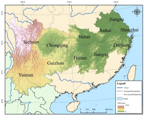
Figure 1.
Geographical location of the YREB.
The YREB can be divided into the upper reaches, middle reaches, and lower reaches according to the differences in geographical conditions and hydrological characteristics. The upper reaches include Sichuan, Chongqing, Yunnan, and Guizhou, containing rich freshwater, minerals, and biological resources. The middle reaches include Hunan, Hubei, and Jiangxi, with many urban agglomerations. The lower reaches include Shanghai, Jiangsu, Zhejiang, and Anhui, the most developed areas on the Yangtze River which play an important role in the economic development of China.
The elevation of the YREB decreases roughly from west to east and has four general terrains: plateaus, mountains, hills, and plains. The whole YREB is vast with a variety of topography and climatic conditions, and the average annual temperature and precipitation in upper, middle, and lower reaches vary drastically from 14.2–17.8 °C and 873.9–2397.5 mm. These factors result in a wealth of habitat types and biodiversity.
2.2. Data Resource
This study used cloudless Landsat TM/OLI images in the growing seasons (May-September) at a 30 m spatial resolution over 2000, 2010, and 2020 to analyze changes in LULC patterns. The data were downloaded from the United States Geological Survey (https://www.usgs.gov/ (last accessed on 11 October 2022)). The 250 m resolution and 16-day MODIS-NDVI data were acquired from the Land Processes Distributed Active Archive Center (https://lpdaac.usgs.gov/products/mod13q1v006/ (last accessed on 11 October 2022)). The daily meteorological data of 1193 stations along the YREB and its surrounding areas used in this study, including precipitation, wind speed, temperature, air pressure, humidity, sunshine, and evaporation data, were downloaded from the China Meteorological Data Service Center (http://data.cma.cn/ (last accessed on 1 October 2022)). The soil map with a scale of 1:1000000 was obtained from the Harmonized World Soil Database (HWSD) (http://www.tpdc.ac.cn/zh-hans/ (last accessed on 11 October 2022)). The Digital Elevation Model (DEM) data with a 30 m spatial resolution were downloaded from the United States Geological Survey (https://www.usgs.gov/ (last accessed on 11 October 2022)). The social, economic, and other dynamic development statistic data came from the local Regional Statistical Yearbook. And, the population density data were downloaded from WorldPop (http://www.worldpop.org/ (last accessed on 11 October 2022)).
2.3. LULC Classification
The images were classified into six types referring to the International Geosphere-Biosphere Program (IGBP) classification in this study, including water, construction land, crop land, forest land, grass land, and bare land. We used the Google Earth Engine (GEE) platform to retrieve and cite the Landsat TM and the OLI image data with 30 × 30 spatial resolutions. Radiometric calibration, atmospheric correction, and cloud removal processing were carried out on the EarthExplorer platform. Then, we selected 80,000 to 100,000 sample points for each selected year, used a random forest classifier to classify the mosaic images, and acquired the LULC maps. Finally, we tested the accuracy of the LULC maps based on the 10,000 permanent monitoring sites in China’s continuous forest inventory from 11 provinces and municipalities. The overall accuracy of the test results indicated that all the LULC maps were above 0.8, which satisfies the requirements of our research.
2.4. ES Supply and Demand
We ran quantitative assessments of the supply and demand of ESs using the following criteria: (1) First, we wanted to assess ESs as comprehensively as possible, so we referred to the ES classification framework from the Common International Classification of Ecosystem Services (CICES) [32]; provisioning, regulating, and cultural services are included in the selection of the ESs in this study. (2) Second, we wanted to assess ESs in which the importance of the services in the region had been recognized by the government [33], i.e., the outline of the YREB development plan points out that the YREB should conserve energy and reduce emissions, pursue low-carbon, and have a circular development. To reduce carbon emissions, local governments have been actively optimizing the industrial structures, planting trees, and conducting afforestation, which can be quantitatively described through the ESs and provide a reference for local governments. (3) Based on the previous two criteria, we need to adjust the selection of ESs to match the data accessibility and model adaptability.
Based on these criteria, we selected five ESs, namely, carbon sequestration (regulating service), soil conservation (regulating service), water retention (regulating service), food production (provisioning service), and recreational opportunity (cultural service). Then, we quantified the supply and demand of them in the YREB.
2.4.1. Carbon Sequestration
The carbon sequestration service supply can be expressed by the net primary productivity (NPP) of the vegetation. NPP indicates the total amount of organic matter accumulated by vegetation, and it was estimated by the Carnegie–Ames–Stanford Approach (CASA) terrestrial carbon model [34] (Equation (1)). The carbon sequestration service demand can be expressed as the local carbon emission which is determined by the standard coal consumption and carbon conversion rate (Equation (2)).
where and , respectively, indicate the carbon sequestration service of supply and demand (ton); is the net primary productivity of LULC type (ton/ha); is the area of LULC type (ha); 1.63 represents the mean capacity of vegetation to absorb carbon through a photosynthesis process [20]; and , , and represent the standard coal consumption for agricultural, industrial, and home (ton). The data for the standard coal consumption was obtained from the statistical yearbooks of each province. Agricultural carbon consumption was allocated equally to croplands, industrial carbon consumption was allocated equally to other artificial lands in construction land, and home carbon consumption was equally allocated to urban and rural lands in construction land on the provincial scale. is the standard coal emission coefficient, 0.68, set by the National Development and Reform Commission.
2.4.2. Soil Conservation
The soil conservation service supply is quantitatively defined as the difference between the potential soil erosion and actual soil erosion, which can generally be calculated by the Revised Universal Soil Loss Equation (RUSLE) model [35] (Equation (3)). The soil conservation service demand is represented as the actual soil erosion in the RUSLE model (Equation (4)).
where and , respectively, indicate the soil conservation service supply and demand (t·hm−2); is the rainfall erosivity ((MJ·mm·hm2·h−1) which was calculated by the monthly rainfall erosivity [36]; is the soil erodibility factor (t·ha·h·MJ−1·mm−1·hm−2) which was obtained by the Erosion–Productivity Impact Calculator (EPIC) [37]; is the topographic factor representing the effect of the regional terrain (slope length and gradient) and is estimated based on the DEM data with a 30 m resolution [38]; is the crop/vegetation and management factor which reflects the effect of surface vegetation on soil erosion reduction; and is the support practice factor, with the value ranging between 0 and 1. In this study, and were selected by the regional research [39].
2.4.3. Water Retention
The water retention service supply represents the water reserves in an ecosystem, and we used the seasonal water retention module in the InVEST model (version 3.8.9) [40] to estimate the regional water retention. This model calculated the annual water recharge on a monthly scale and can be expressed as Equation (5). The water retention service demand was based on the regional water use status and the LULC types (Equation (6)) [20]. The consumption of water resources mainly included four parts, including agricultural water, industrial water, home water, and ecological water. We collected the water resource bulletins of different provinces from 2000 to 2020, and the spatial distribution of the amount of water demand was mapped out by equally distributing the water consumption of different uses on the corresponding LULC types.
where is the water retention service supply (m3); is the annual precipitation (mm) which is represented by the monthly precipitation and obtained from daily precipitation data; and is the quick flow (mm), which represents the generation of streamflow with watershed residence times of hours to days [40]. In this study, was determined by the monthly rainfall, the number of rainy days, LULC patterns, and soil properties. is the actual evapotranspiration (mm) which is based on the improved Penman–Monteith formula [41]; is the water retention service demand (m3); and , , , and represent the water consumption for agricultural, industrial, home, and ecological, respectively (m3). Due to the availability of data, agricultural water consumption was equally allocated to croplands, industrial water consumption was equally allocated to other artificial lands in construction land, home water consumption was equally allocated to urban and rural lands in construction land, and ecological water consumption was equally allocated to forest land and grass land on the provincial scale.
2.4.4. Food Production
The food production service supply was indicated by the mean food value per pixel (yuan/hm2). Food production was divided into four industries including agriculture, forestry, fishery, and animal husbandry, which are distributed on croplands, forest land, water, and grass land, respectively. The fishery production value was equally allocated to water. The agriculture, forestry, and animal husbandry production values were calculated by NDVI (Equation (7)). The food production service demand was represented as the grain consumed per person in each year (Equation (8)).
where is the food production service supply (yuan/hm2); is the NDVI value of industry in units of ; is the sum of NDVI in industry ; is the sum of the production value in industry ; is the food production service demand (yuan/hm2); is the population density (person/hm2); and is the per capita grain consumption of residents (yuan/person) which was obtained from the statistical yearbooks of the provinces in the YREB. In addition, considering the availability of data, FPS and FPD were calculated at the provincial scale, and then we conducted the analysis.
2.4.5. Recreational Opportunity
The recreational opportunity service supply was measured by the proportion of forest land and grass land [20] (Equation (9)). Considering the basic units of government administration and the availability of the data, the county was regarded as the spatial unit in the evaluation of the recreational opportunity service supply. The recreational opportunity service demand is expressed as the residents’ demand for public green spaces and is calculated by the population density and the per capita green area, as determined by the local government. Considering that the supply of the recreational opportunity service was evaluated at the county level, we improved the formula on the basis of Chen et al. [20] and also evaluated the recreational opportunity service demand at the county level. (Equation (10)).
where expresses the recreational opportunity service supply (km2/km2); and are the area of forest land and grass land in county ‘’ (km2), respectively; is the area of county ‘’ (km2); is the recreational opportunity service demand (km2/km2); is the population in county ‘’ (person); and is the per capita green area determined in the 14th Five-Year Plan of China, set at 20 m2/person.
2.4.6. ES Supply and Demand Match
The ecological supply–demand ratio (ESDR) links the actual supply and demand of ESs. The ESDR is often used to represent the surplus or deficit of regional ESs [42] (Equation (11)).
where and respectively indicate the supply and demand of the ES type in units of . The and refer to the maximum values of actual supply and demand in the ES type , respectively. A positive value of the indicates a surplus state of the ES type supply and demand, a negative value indicates a deficit state, and a value ranging from −0.001 to 0.001 indicates a balanced state of the ES type supply and demand because of the few regions which meet the standard balance of the supply and demand. In addition, since the supply–demand of the recreational opportunity services was evaluated at the county scale, the ESDR of the recreational opportunity service was represented as the difference between supply and demand in each county, respectively.
In order to characterize the coordination between the supply and demand of ESs at the integral level, we calculated the comprehensive supply–demand ratio () using Equation (12) [20]:
where is the number of ES types and is the ecological supply–demand ratio of the ES type . In the calculation results of Equation (12), the CESDR is calculated by the arithmetic mean of ESDR to indicate the total state of the regional ESs at the county scale; a positive value of the CESDR indicates a surplus state of the ES supply and demand, a negative value indicates a deficit state, and a value ranging from −0.001 to 0.001 indicates a balanced state of the ES supply and demand.
2.5. Spatial Autocorrelation Analysis
Based on the relevant research [23,43], the comprehensive urbanization level (CUL) of the YREB was measured by three aspects: population urbanization, economic urbanization, and landscape urbanization. Population density (person/km2) was selected to reflect population urbanization, GDP density (104 yuan/km2) was used to measure economic urbanization, and the proportion of construction land in each county (%) was applied to describe landscape urbanization. Finally, we used the average value of the three normalized indexes as the indicator to measure the level of urbanization development.
We applied the bivariate Moran’s I to explore the spatial correlation between the CESDR and CUL in the YREB. The bivariate Moran’s I includes the global bivariate Moran’s I and the local bivariate Moran’s I. Global bivariate Moran’s I reveals the overall spatial correlations between the CESDR and UCL, in which values range from −1 to 1, and a higher absolute value indicates a stronger spatial correlation. A positive value reflects a positive spatial correlation, a negative value indicates a negative correlation, and zero means no spatial autocorrelation whatsoever [28,44]. The local bivariate Moran’s I explains the spatial correlations among different spatial units [45]. The clustering maps generated by local bivariate Moran’s I methods can reveal the spatial aggregation relationship among different spatial units in the ES supply–demand mismatch and the urbanization level from five aspects: high–high (HH, high CESDR value surrounded by high CUL), low–low (LL, low CESDR value surrounded by low CUL), high–low (HL, high CESDR value surrounded by low CUL), low–high (LH, low CESDR value surrounded by high CUL), and no relationship.
3. Results
3.1. LULC Change
The LULC of the YREB has demonstrably changed over the past 20 years (Figure 2). The proportion results of different LULC types in each period show that forest land, crop land, and grass land areas accounted for the most abundant, followed by construction land, water, and bare land. The areas of construction land, crop land, and forest land changed dramatically, while grass land, bare land, and water areas’ changes were fewer. Among all, the expansion trend of construction land was the most obvious, which increased from 23,528 km2 (1.15%) in 2000 to 66,537 km2 (3.24%) in 2020 and mainly occurred in the YREB development zone in the lower reaches (Table 1). The proportion of forest land without great changes went from 48.68% to 53.84% but has increased by about 105,000 km2 in the past 20 years. The negative change in crop land was the most prominent, with a change rate of −20.1%, and it was mainly converted into construction land. In addition, the change rates of water, bare land, and grass land were 9.25%, 9.57%, and −8.17%, respectively.
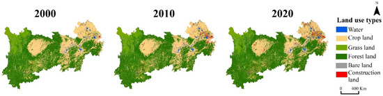
Figure 2.
Spatial distribution of the LULC in the YREB from 2000 to 2020.

Table 1.
The land use patterns change from 2000 to 2020 in the YREB (km2).
3.2. ES Supply and Demand
The quantitative evaluation results of supply, demand, and ESDR showed that the ESs were different in spatial distribution and had changed obviously from 2000 to 2020 (Figure 3, Figure 4, Figure 5 and Figure 6). The total supply of the carbon sequestration service in the YREB increased by 36.99%, from 1.54 billion tons in 2000 to 2.11 billion tons in 2020, and the total demand of the carbon sequestration service also showed an increasing trend from 0.59 billion tons in 2000 to 1.63 billion tons in 2020, with an increase of 177.10%. The increase rate of the total demand was higher than that of the total supply of the carbon sequestration. Although the total supply was significantly greater than the total demand, there is still an obvious mismatch between the supply and demand in some regions. (Figure 3). Higher supply areas of carbon sequestration services were mostly distributed in forest land and grass land, which were also in low-demand areas which have an overall surplus. Whereas, the surplus of carbon sequestration has been halved, this result leads to an obvious expansion trend in the deficit areas, and the deficit situation became worse in the low-supply but high-demand areas, such as on industrial lands and urban lands.
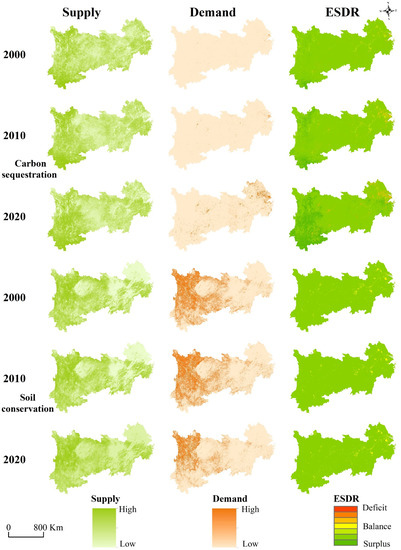
Figure 3.
Spatial distribution of supply (left column), demand (middle column), and ESDR (right column) for carbon sequestration and soil conservation in the YREB from 2000 to 2020.
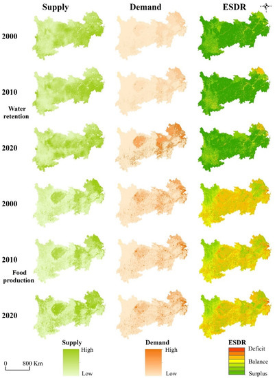
Figure 4.
Spatial distribution of supply (left column), demand (middle column), and ESDR (right column) for water retention and food production in the YREB from 2000 to 2020.
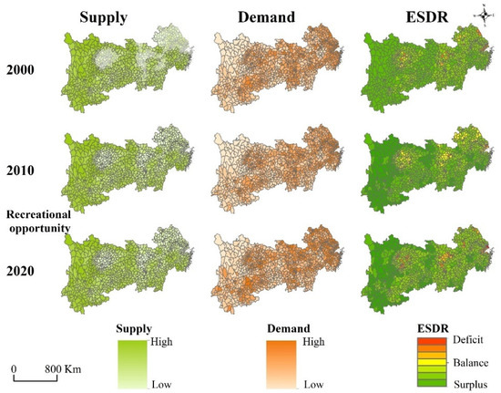
Figure 5.
Spatial distribution of supply (left column), demand (middle column), and ESDR (right column) for recreational opportunities in the YREB from 2000 to 2020.
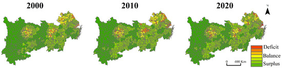
Figure 6.
Spatial distribution of CESDR in the YREB from 2000 to 2020.
The total soil conservation service supply showed an increasing trend from 23.45 billion tons in 2000 to 31.37 billion tons in 2020, with an increase of 33.77%. At the same time, soil conservation service demand also increased from 0.64 billion tons in 2000 to 0.87 billion tons in 2020, with an increase of 35.93%. The spatial distribution of the balanced and the deficit areas remained nearly unchanged when the water and urban agglomeration were in the higher deficit region of the soil conservation service (Figure 3). In addition, the shortfall areas were expanded by 7.36% over the past 20 years. In addition, the balanced areas of the soil conservation service were mainly distributed in the crop lands of the middle and lower reaches, and a part of the balanced areas had transitioned to a surplus in the YREB.
The total water retention service supply exceeded the demand over the entire period, and the surplus was 742.30 billion m3 in 2000, 619.87 billion m3 in 2010, and 643.63 billion m3 in 2020. The total supply of the water retention service decreased from 973.82 billion m3 in 2000 to 908.14 billion m3 in 2020, with a decrease of 6.74%. However, the total demand of the water retention service increased markedly from 231.52 billion m3 in 2000 to 264.51 billion m3 in 2020, with an increase of 14.24%. The surplus advantage was decreasing, and the overall surplus situation did not mean that the spatial distribution of the supply and demand was equal. The spatial mismatch changed greatly over different periods (Figure 4). The high-supply areas of the water retention service were mainly distributed in the middle reaches and lower reaches of the YREB, where they have higher precipitation compared to the upper reaches. Due to the high population density and industrial development, the demand for the water retention service in industrial lands and urban areas was more clustered, and with the development of agriculture, the demand for water resources from the lower reaches also increased. These results aggravated the mismatch between the supply and demand of the water retention service in the YREB.
The supply and demand of the food production service has improved dramatically over the past 20 years. Supply for the food production service has increased from 1046.76 billion yuan in 2000 to 5801.13 billion yuan in 2020, which means it has expanded about fivefold. In addition, the total demand for food production service increased from 2485.37 billion yuan in 2000 to 14,660.80 billion yuan in 2020, with an expansion that was about sixfold. Obviously, the food supplies cannot satisfy the food needs in the YREB, and the spatial distribution of the food production service supply and demand was mismatched (Figure 4). Crop lands are the major food-producing areas, and they have the prominent capacity of providing food, so most crop land areas were in surplus. Construction lands with a high population density showed a higher demand for food, where there was also the most serious deficit, and this deficit showed an increasing trend from 2000 to 2020. The food supply of forest land in the upper and middle reaches was lower than the human needs, but these shortfall areas have shrunken since 2010.
In the process of economic development, the total demand of the recreational opportunity service increased from 15,146.43 km2 in 2000 to 16,055.71 km2 in 2020, with the expansion of the population density in the YREB. In addition, with the increase in grass land and forest land from 1,308,582 km2 in 2000 to 1,387,981 km2 in 2020, the total supply of recreational opportunity service also showed an increasing trend. Thus, there was no shortfall in the recreational opportunity service in the entire total of the YREB. However, compared to the total surplus, there was still a spatial mismatch condition in the local supply and demand (Figure 5). In general, the number of deficit counties greatly increased from 114 in 2000 to 157 in 2020, and the increased areas were mainly clustered in the three urban agglomerations from the upper, middle, and lower reaches, while the most serious deficit situation was in 2010 with 187 counties. Moreover, some counties in the upper and lower reaches had transitioned from deficit to surplus, which was most pronounced between 2010 and 2020.
In the past 20 years, the spatial pattern of the ES supply and demand has changed dramatically, and the spatial mismatch is serious, especially in the regions where an ES supply and demand deficit occurs (Figure 6). Among them, areas with significant surplus in ES supply and demand were mainly located in the counties with more forest and grass areas, which were in the upper reaches and were relatively stable. These were the key areas of national environmental protection because of their fragile ecological environments. In comparison, the supply and demand deficit areas were mainly distributed in urban areas and were increasingly concentrated in metropolitan areas, which increased from 115 in 2000 to 165 in 2020, and most of the augmentations were converted from supply and demand balance areas. However, there are still some deficit counties turning into surplus; these counties are mainly surrounded metropolitan areas. In addition, the supply and demand balance areas were mainly distributed in crop lands, where they have a lower population density and are the most important grain supply areas in the whole YREB. The gap between the ES supply and human demand was narrower.
3.3. The Spatial Relationship between the CUL and the CESDR
The global bivariate Moran’s I analysis revealed significant negative spatial correlations between the CESDR and the CUL at the different stages (all Moran’s I values < 0 and p-values < 0.001) (Figure 7). The Moran’s I value decreased from −0.424 in 2000 to −0.497 in 2010 and to −0.531 in 2020. This result indicated that with the increase in urbanization in a location, the CESDR in the surrounding areas may deteriorate. Moreover, the clustering between the CESDR and the CUL tended to be strong (the absolute value of the z-value increased), and most points were distributed in the second and fourth quadrants. The local bivariate Moran’s I map displayed the spatial clustering effect between the CESDR and the CUL from five aspects, and this clustering pattern had obvious similarities in the different periods (Figure 8).
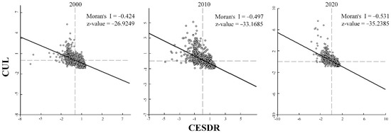
Figure 7.
Scatter plot of Moran’s I index between the CESDR and the CUL in the YREB from 2000 to 2020.
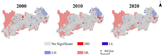
Figure 8.
The local bivariate Moran’s I clustering graph between the CESDR and the CUL in the YREB from 2000 to 2020. (CESDR: comprehensive supply–demand ratio; CUL: comprehensive urbanization level; HH: high CESDR value and high CUL; HL: high CESDR value and low CUL; LH: low CESDR value and high CUL; LL: low CESDR value and low CUL).
HL areas were distributed across a large area and have shown an expanding trend in over the past 20 years, which mainly distributed grass land and forest land in the upper reaches, and some counties with higher vegetation coverage in the middle and lower reaches. LH areas were mainly clustered in the three urban agglomerations within highly developed cities in the YREB, and a contraction from the periphery to the central area during the study periods. In addition, the areas of HH were not widely distributed and were primarily around LH areas, which means that these counties had a better balance between urban development and ES supply–demand. The proportion of the LL areas was the lowest, and it was distributed sporadically along the YREB. These counties and districts were mainly distributed in the lower reaches, where there was a higher proportion of crop land areas, the level of urbanization and population density were lower, and the gap between the supply from ESs and the demand from humans was lowest.
4. Discussion
4.1. The Impact of Urbanization on the Supply and Demand of Ecosystem Services
Our research suggests that the mismatch between supply and demand of the ESs became a serious problem in the YREB from 2000 to 2020, and the negative effects of urbanization on the ES supply–demand mismatch started to increase gradually. A possible reason for the negative effects of the CUL on the CESDR was that urbanization disrupted the energy exchange and the material cycle of the natural ecosystem, which curtails the ES supply with the dramatic change in LULC. However, with the increasing population in the metropolitan areas, the demand for various services has begun to constantly increase, which has made the regional ES deficit situation worse, especially in metropolitan areas [46]. Similar studies also have suggested that urbanization and the ESs were correlated, rather than being independent. Urbanization and human interferences were the main factors of regional ES degradation [47,48]. One unexpected finding was that the deterioration of the mismatch between ES supply and demand is not irreversible at the county scale, and the ESs of some better-developed counties have transformed from a deficit to a surplus. A possible explanation for this result is that reasonable urban planning and positive human interferences may play an important role in balancing economic and sustainable development, which has been ignored frequently in previous studies. For example, a total of 11.84 million hectares of forest have been planted in the 30 years since China launched the Yangtze River Basin shelterbelt system construction project in 1989, and ecosystem services have been greatly improved [49]. The results of the local bivariate Moran’s I showed that the spatial clustering relationships of some regions had changed from LH to HH with economic development, which proved that there can also be a positive effect of urbanization on the balance of the ES supply–demand in local counties. For instance, Wenzel et al. showed that urbanization enhanced pollinator diversity compared to intensified agricultural landscapes; pollinator diversity generally increased with the amount of urban green space [50]. The shrinking trend of the LH regions from the periphery to the central area during the study period also means that the process of urbanization in central urban areas has an influence on the entire clustering results. These results explain why the relative value of the bivariate of Moran’s I has been increasing but the deficit areas cluster from all sides towards metropolitan areas from 2000 to 2020.
Although urbanization had a negative spatial spillover effect on the supply and demand of ESs as a whole, the response between the UCL and the CESDR was not uniform at the county scale. The results of local bivariate Moran’s I demonstrated that the spatial clustering formed between the ES supply–demand mismatch and the urbanization level have significant regional differences at different periods in the YREB. With the development of urban areas, the most obvious change was that LH regions were gradually concentrated in the Yangtze River Delta urban agglomeration, Chengdu–Chongqing urban agglomeration, Wuhan urban agglomeration, and Chang-Zhu-Tan urban agglomeration. The counties in the middle and lower reaches with relatively slow urbanization gradually changed from LH to insignificant. According to existing research, this result may be related to the concentration of urban industrial chains, regional urban governance and planning, and the influence of non-urbanization factors such as vegetation coverage and precipitation on the ES supply-demand [51]. Our results were also consistent with previous studies and indicated that, although urbanization is the most important factor affecting the regional supply and demand of ESs, ecosystems are being changed by a combination of natural factors and human disturbances [52,53]. Positive human disturbances may promote the sustainable development of regional ESs. For example, in the process of the urbanization of the Anji county, the vegetation area proportion has been stable at 60%, which can provide a good recreational opportunity service and soil conservation service for the regional areas. This county also vigorously developed intensive agriculture, adhered to the red line of cultivated land, and secured the residents’ demand for food. Thus, the relationship between ES supply and demand was at a surplus in the Anji county.
4.2. Limitations and Implications for Future Research
Our research explored the complex relationship between the ES supply–demand mismatch and urbanization and improved the existing indicator for calculating the recreational opportunity service to make it more suitable for different scales. However, this work still has some limitations and uncertainties. Firstly, the consistent expression of different ESs at the same spatial scale will cause some errors in calculation. For example, the data on the food production service supply are mainly collected and calculated at the provincial scale due to the availability of data, so even the downscaling calculation based on the NDVI will lead to some uncertainties in the results at the county scale.
Secondly, our research relied on the use of models and algorithms, which have their own uncertainties. For example, the contributions of grass land and forest land were only considered due to the lack of potential indicators of human water demand, while the contribution of the water body was ignored when estimating the supply and demand for recreational opportunity services.
Thirdly, the scale effect was always used to analyze differences in the results when spatial units or ranges changed, but this study only conducted a single spatial scale analysis of the relationship between the ES supply–demand mismatch and urbanization, which made it difficult to verify and apply the results at different spatial scales [28,54]. ES supply and demand may have different spatial distribution and equilibrium relationships according to different scales. Therefore, exploring the spatial aggregation patterns between the ES supply–demand mismatch and urbanization from the perspective of multiple scales will become the focus in the future.
Finally, we found that the ESs switch between surpluses and deficits in some counties surrounding metropolitan areas. This is in contrast to the deteriorating deficits in metropolitan areas, but we did not specifically analyze the driving mechanism of this condition. We also ignored the economic value of ESs’ status change. Therefore, further research should be undertaken to prove the positive effects of human activities on the ecosystem by selecting typical counties to explore the impact of human disturbances and climate change on the ES supply–demand.
5. Conclusions
In this study we quantified the supply, demand, and mismatches of the five ESs in the YREB, using the bivariate Moran’s I to investigate the impact of urbanization on the ES supply–demand mismatch at the county scale from 2000 to 2020. This study showed that the growth gap between the total supply and the total demand of ESs led to a growing spatial mismatch of the ES supply–demand from 2000 to 2020, especially in metropolitan areas. The rapid urbanization caused by population, economy, and urban expansion has had an intensified negative impact on the ES supply–demand. However, the spatial correlations between the urbanization levels and ES supply–demand mismatch are not unique. Furthermore, the spatial clustering results are changing dynamically at the county scale. In particular, the clustering situation in some areas will be improved with the development of urbanization. Consequently, in the process of urban development, human demands should be taken into account when the government manages, and it should attempt to balance the ES supply–demand and urbanization to achieve more sustainable development.
Author Contributions
Conceptualization, H.L. and J.Z.; methodology, H.L.; software, Q.L.; validation, H.L., L.Z. and Q.L.; formal analysis, H.L.; investigation, W.X.; resources, Q.L.; data curation, L.Z.; writing—original draft preparation, H.L.; writing—review and editing, J.Z.; visualization, W.X.; supervision, W.X.; project administration, J.Z.; funding acquisition, J.Z. All authors have read and agreed to the published version of the manuscript.
Funding
This study was supported by the program of the Fundamental Research Funds of Chinese Academy of Forestry (Grant No. CAFYBB2019ZD001) and the National Key Research and Development Program of China (2016YFD0600206).
Data Availability Statement
Not applicable.
Acknowledgments
We greatly appreciate the National Forest Ecosystem Station of Three Gorges Reservoir in Zigui County. Special thanks to the editors and reviewers for providing valuable insight into this article.
Conflicts of Interest
The authors declare no conflict of interest.
References
- Costanza, R.; d’Arge, R.; de Groot, R.; Farber, S.; Grasso, M.; Hannon, B.; Limburg, K.; Naeem, S.; O’Neill, R.V.; Paruelo, J.; et al. The value of the world’s ecosystem services and natural capital. Nature 1997, 387, 253–260. [Google Scholar] [CrossRef]
- Zhang, Z.M.; Peng, J.; Xu, Z.H.; Wang, X.Y.; Meersmans, J. Ecosystem services supply and demand response to urbanization: A case study of the Pearl River Delta, China. Ecosyst. Serv. 2021, 49, 101274. [Google Scholar] [CrossRef]
- Gret-Regamey, A.; Huber, S.H.; Huber, R. Actors’ diversity and the resilience of social-ecological systems to global change. Nat. Sustain. 2019, 2, 290–297. [Google Scholar] [CrossRef]
- MEA. Millennium Ecosystem Assessment: Ecosystems and Human Well-Being; Island Press: Washington, DC, USA, 2005. [Google Scholar]
- Romulo, C.L.; Posner, S.; Cousins, S.; Fair, J.H.; Bennett, D.E.; Huber-Stearns, H.; Richards, R.C.; McDonald, R.I. Global state and potential scope of investments in watershed services for large cities. Nat. Commun. 2018, 9, 4375. [Google Scholar] [CrossRef] [PubMed]
- Kroll, F.; Mueller, F.; Haase, D.; Fohrer, N. Rural-urban gradient analysis of ecosystem services supply and demand dynamics. Land Use Policy 2012, 29, 521–535. [Google Scholar] [CrossRef]
- Dai, X.; Wang, L.C.; Tao, M.H.; Huang, C.B.; Sun, J.; Wang, S.Q. Assessing the ecological balance between supply and demand of blue-green infrastructure. J. Environ. Manag. 2021, 288, 112454. [Google Scholar] [CrossRef] [PubMed]
- Seto, K.C.; Güneralp, B.; Hutyra, L.R. Global forecasts of urban expansion to 2030 and direct impacts on biodiversity and carbon pools. Proc. Natl. Acad. Sci. USA 2012, 109, 16083–16088. [Google Scholar] [CrossRef] [PubMed]
- United Nations. World Urbanization Prospects: 2014 Revision, Department of Economic and Social Affairs, Population Division; United Nations: New York, NY, USA, 2014. [Google Scholar]
- Alemu, I.J.B.; Richards, D.R.; Gaw, L.Y.-F.; Masoudi, M.; Nathan, Y.; Friess, D.A. Identifying spatial patterns and interactions among multiple ecosystem services in an urban mangrove landscape. Ecol. Indic. 2021, 121, 107042. [Google Scholar] [CrossRef]
- Yuan, Y.J.; Wu, S.H.; Yu, Y.N.; Tong, G.J.; Mo, L.J.; Yan, D.H.; Li, F.F. Spatiotemporal interaction between ecosystem services and urbanization: Case study of Nanjing City, China. Ecol. Indic. 2018, 95, 917–929. [Google Scholar] [CrossRef]
- Qiu, B.; Li, H.; Zhou, M.; Zhang, L. Vulnerability of ecosystem services provisioning to urbanization: A case of China. Ecol. Indic. 2015, 57, 505–513. [Google Scholar] [CrossRef]
- Wang, Z.F. Evolving landscape-urbanization relationships in contemporary China. Landsc. Urban Plan. 2018, 171, 30–41. [Google Scholar] [CrossRef]
- Burkhard, B.; Kroll, F.; Nedkov, S.; Muller, F. Mapping ecosystem service supply, demand and budgets. Ecol. Indic. 2012, 21, 17–29. [Google Scholar] [CrossRef]
- Kremer, P.; Hamstead, Z.; Haase, D.; McPhearson, T.; Frantzeskaki, N.; Andersson, E.; Kabisch, N.; Larondelle, N.; Lorance Rall, E.; Voigt, A. Key insights for the future of urban ecosystem services research. Ecol. Soc. 2016, 21, 29. [Google Scholar] [CrossRef]
- Estoque, R.C.; Murayama, Y. Landscape pattern and ecosystem service value changes: Implications for environmental sustainability planning for the rapidly urbanizing summer capital of the Philippines. Landsc. Urban Plan. 2013, 116, 60–72. [Google Scholar] [CrossRef]
- Qiu, S.J.; Ding, Z.H.; Liu, H.Y.; Peng, J.; Zhang, H.B.; Quine, T.A.; Dong, J.Q.; Mao, Q.; Meersmans, J.; Wang, X.Y. Understanding the relationships between ecosystem services and associated social-ecological drivers in a karst region: A case study of Guizhou Province, China. Prog. Phys. Geogr. 2021, 45, 98–114. [Google Scholar] [CrossRef]
- Cao, T.G.; Yi, Y.J.; Liu, H.X.; Xu, Q.; Yang, Z.F. The relationship between ecosystem service supply and demand in plain areas undergoing urbanization: A case study of China’s Baiyangdian Basin. J. Environ. Manag. 2021, 289, 112492. [Google Scholar] [CrossRef] [PubMed]
- González-García, A.; Palomo, I.; González, J.A.; López, C.A.; Montes, C. Quantifying spatial supply-demand mismatches in ecosystem services provides insights for land-use planning. Land Use Policy 2020, 94, 104493. [Google Scholar] [CrossRef]
- Chen, J.; Jiang, B.; Bai, Y.; Xu, X.B.; Alatalo, J.M. Quantifying ecosystem services supply and demand shortfalls and mismatches for management optimisation. Sci. Total Environ. 2019, 650, 1426–1439. [Google Scholar] [CrossRef]
- Bing, Z.H.; Qiu, Y.S.; Huang, H.P.; Chen, T.Z.; Zhong, W.; Jiang, H. Spatial distribution of cultural ecosystem services demand and supply in urban and suburban areas: A case study from Shanghai, China. Ecol. Indic. 2021, 127, 107720. [Google Scholar] [CrossRef]
- Lin, J.Y.; Huang, J.L.; Prell, C.; Bryan, B.A. Changes in supply and demand mediate the effects of land-use change on freshwater ecosystem services flows. Sci. Total Environ. 2021, 763, 143012. [Google Scholar] [CrossRef]
- Peng, J.; Wang, X.Y.; Liu, Y.X.; Zhao, Y.; Xu, Z.H.; Zhao, M.Y.; Qiu, S.J.; Wu, J.S. Urbanization impact on the supply-demand budget of ecosystem services: Decoupling analysis. Ecosyst. Serv. 2020, 44, 101139. [Google Scholar] [CrossRef]
- Peng, J.; Tian, L.; Liu, Y.X.; Zhao, M.Y.; Hu, Y.N.; Wu, J.S. Ecosystem services response to urbanization in metropolitan areas: Thresholds identification. Sci. Total Environ. 2017, 607, 706–714. [Google Scholar] [CrossRef]
- Ye, Y.Q.; Bryan, B.A.; Zhang, J.E.; Connor, J.D.; Chen, L.L.; Qin, Z.; He, M.Q. Changes in land-use and ecosystem services in the Guangzhou-Foshan Metropolitan Area, China from 1990 to 2010: Implications for sustainability under rapid urbanization. Ecol. Indic. 2018, 93, 930–941. [Google Scholar] [CrossRef]
- He, Y.Y.; Kuang, Y.Q.; Zhao, Y.L.; Ruan, Z. Spatial Correlation between Ecosystem Services and Human Disturbances: A Case Study of the Guangdong–Hong Kong–Macao Greater Bay Area, China. Remote Sens. 2021, 13, 1174. [Google Scholar] [CrossRef]
- Baró, F.; Palomo, I.; Zulian, G.; Vizcaino, P.; Haase, D.; Gómez-Baggethun, E. Mapping ecosystem service capacity, flow and demand for landscape and urban planning: A case study in the Barcelona metropolitan region. Land Use Policy 2016, 57, 405–417. [Google Scholar] [CrossRef]
- Zhang, Y.; Liu, Y.F.; Zhang, Y.; Liu, Y.; Zhang, G.X.; Chen, Y.Y. On the spatial relationship between ecosystem services and urbanization: A case study in Wuhan, China. Sci. Total Environ. 2018, 637, 780–790. [Google Scholar] [CrossRef] [PubMed]
- Zhang, H.; Gao, J.X.; Qiao, Y.J. Current situation, problems and suggestions on ecology and environment in the Yangtze River Economic Belt. Environ. Dev. Sustain. 2019, 44, 28–32. (In Chinese) [Google Scholar] [CrossRef]
- Kong, L.Q.; Zheng, H.; Xiao, Y.; Ouyang, Z.Y.; Li, C.; Zhang, J.J.; Huang, B.B. Mapping Ecosystem Service Bundles to Detect Distinct Types of Multifunctionality within the Diverse Landscape of the Yangtze River Basin, China. Sustainability 2018, 10, 857. [Google Scholar] [CrossRef]
- Ministry of Ecology and Environment of the People’s Republic of China, National Development and Reform Commission, Ministry of Water Resources. Environmental Protection Plan for the Yangtze River Economic Belt; Ministry of Ecology and Environment of the People’s Republic of China, National Development and Reform Commission, Ministry of Water Resources: Beijing, China, 2017.
- Haines-Young, R.; Potschin-Young, M. Revision of the common international classification for ecosystem services (CICES V5.1): A policy brief. One Ecosyst. 2018, 3, e27108. [Google Scholar] [CrossRef]
- Sun, X.; Lu, Z.M.; Li, F.; Crittenden, J.C. Analyzing spatio-temporal changes and trade-offs to support the supply of multiple ecosystem services in Beijing, China. Ecol. Indic. 2018, 94, 117–129. [Google Scholar] [CrossRef]
- Potter, C.S.; Randerson, J.T.; Field, C.B.; Matson, P.A.; Vitousek, P.M.; Mooney, H.A.; Klooster, S. Terrestrial ecosystem production: A process model based on global satellite and surface data. Glob. Biogeochem. Cycle 1993, 7, 811–841. [Google Scholar] [CrossRef]
- Renard, K.G.; Foser, G.R.; Weesies, G.A.; Mccool, D.K.; Yoder, D.C. Predicting Soil Erosion by Water: A Guide to Conservation Planning with the Revised Universal Soil Loss Equation (RUSLE); United States Department of Agriculture: Washington, DC, USA, 1997; p. 703.
- Zhang, W.B.; Xie, Y.; Liu, B.Y. Rainfall Erosivity Estimation Using Daily Rainfall Amounts. Sci. Geogr. Sin. 2003, 22, 705–711. (In Chinese) [Google Scholar]
- Williams, J.R.; Renard, K.G.; Dyke, P.T. EPIC: A new method for assessing erosion’s effect on soil productivity. J. Soil Water Conserv. 1983, 38, 381–383. [Google Scholar]
- Rao, E.M.; Ouyang, Z.Y.; Yu, X.X.; Xiao, Y. Spatial patterns and impacts of soil conservation service in China. Geomorphology 2014, 207, 64–70. [Google Scholar] [CrossRef]
- Jin, Y. Quantitative Study of Ecological Compensation at Multiple Spatial and Temporal Scales; Zhejiang University: Zhejiang, China, 2009. (In Chinese) [Google Scholar]
- Sharp, R.; Douglass, J.; Wolny, S.; Arkema, K.; Bernhardt, J.; Bierbower, W.; Chaumont, N.; Denu, D.; Fisher, D.; Glowinski, K.; et al. InVEST 3.12.0 User’s Guide; The Natural Capital Project, Stanford University, University of Minnesota, The Nature Conservancy, and World Wildlife Fund: Gland, Switzerland, 2020; Available online: https://storage.googleapis.com/releases.naturalcapitalproject.org/invest-userguide/latest/index.html#invest-models (accessed on 11 October 2022).
- Yin, Y.H.; Wu, S.H.; Zheng, D.; Yang, Q.Y. Radiation calibration of FAO56 Penman-Monteith model to estimate reference crop evapotranspiration in China. Agric Water Manag. 2008, 95, 77–84. [Google Scholar] [CrossRef]
- Li, J.H.; Jiang, H.W.; Bai, Y.; Alatalo, J.M.; Li, X.; Jiang, H.W.; Liu, G.; Xu, J. Indicators for spatial–temporal comparisons of ecosystem service status between regions: A case study of the Taihu River Basin, China. Ecol. Indic. 2016, 60, 1008–1016. [Google Scholar] [CrossRef]
- Li, H.L.; Peng, J.; Liu, Y.X.; Hu, Y.N. Urbanization impact on landscape patterns in Beijing City, China: A spatial heterogeneity perspective. Ecol. Indic. 2017, 82, 50–60. [Google Scholar] [CrossRef]
- Degefu, M.A.; Argaw, M.; Feyisa, G.L.; Degefa, S. Dynamics of urban landscape nexus spatial dependence of ecosystem services in rapid agglomerate cities of Ethiopia. Sci. Total Environ. 2021, 798, 149192. [Google Scholar] [CrossRef] [PubMed]
- Anselin, L.; Rey, S.J. Modern Spatial Econometrics in Practice: A Guide to GeoDa, GeoDaSpace and PySAL; GeoDa Press: Chicago, IL, USA, 2014. [Google Scholar]
- Xue, D.; Wang, Z.J.; Li, Y.; Liu, M.X.; Wei, H.J. Assessment of Ecosystem Services Supply and Demand (Mis)matches for Urban Ecological Management: A Case Study in the Zhengzhou-Kaifeng-Luoyang Cities. Remote Sens. 2022, 14, 1703. [Google Scholar] [CrossRef]
- Wei, H.J.; Xue, D.; Huang, J.C.; Liu, M.X.; Li, L. Identification of Coupling Relationship between Ecosystem Services and Urbanization for Supporting Ecological Management: A Case Study on Areas along the Yellow River of Henan Province. Remote Sens. 2022, 14, 2277. [Google Scholar] [CrossRef]
- Chi, Y.; Shi, H.H.; Zheng, W.; Sun, J.K.; Fu, Z.Y. Spatiotemporal characteristics and ecological effects of the human interference index of the Yellow River Delta in the last 30 years. Ecol. Indic. 2018, 89, 880–892. [Google Scholar] [CrossRef]
- Qin, Q.F.; Chen, C.; Zeng, X.Z.; He, J.F. Review and prospect of protection forest system construction in the Yangtze River Basin in the past 30 years. Sci. Soil Water Conserv. 2018, 16, 145–152. [Google Scholar] [CrossRef]
- Wenzel, A.; Grass, I.; Belavadi, V.V.; Tscharntke, T. How urbanization is driving pollinator diversity and pollination—A systematic review. Biol. Conserv. 2020, 241, 108321. [Google Scholar] [CrossRef]
- Alvarez-Vargas, F.J.; Castano, M.A.V.; Restrepo, C. Demand for Ecosystem Services Drive Large-Scale Shifts in Land-Use in Tropical Mountainous Watersheds Prone to Landslides. Remote Sens. 2022, 14, 3097. [Google Scholar] [CrossRef]
- Amundson, R.; Berhe, A.A.; Hopmans, J.W.; Olson, C.; Sztein, A.E.; Sparks, D.L. Soil and human security in the 21st century. Science 2015, 348, 1261071. [Google Scholar] [CrossRef]
- Fu, J.; Zhang, Q.; Wang, P.; Zhang, L.; Tian, Y.Q.; Li, X.R. Spatio-Temporal Changes in Ecosystem Service Value and Its Coordinated Development with Economy: A Case Study in Hainan Province, China. Remote Sens. 2022, 14, 970. [Google Scholar] [CrossRef]
- Chen, W.X.; Zeng, J.; Chu, Y.M.; Liang, J.L. Impacts of Landscape Patterns on Ecosystem Services Value: A Multiscale Buffer Gradient Analysis Approach. Remote Sens. 2021, 13, 2551. [Google Scholar] [CrossRef]
Publisher’s Note: MDPI stays neutral with regard to jurisdictional claims in published maps and institutional affiliations. |
© 2022 by the authors. Licensee MDPI, Basel, Switzerland. This article is an open access article distributed under the terms and conditions of the Creative Commons Attribution (CC BY) license (https://creativecommons.org/licenses/by/4.0/).