Article

Vegetation Mapping with Random Forest Using Sentinel 2 and GLCM Texture Feature—A Case Study for Lousã Region, Portugal

by
Pegah Mohammadpour
1,2,*,
Domingos Xavier Viegas
1 and
Carlos Viegas
1
1
Univ of Coimbra, ADAI, Department of Mechanical Engineering, Rua Luís Reis Santos, Pólo II, 3030-788 Coimbra, Portugal
2
Universidad de Alcala, Environmental Remote Sensing Research Group, Department of Geology, Geography and Environment, Colegios 2, 28801 Alcalá de Henares, Spain
*
Author to whom correspondence should be addressed.
Remote Sens. 2022, 14(18), 4585; https://doi.org/10.3390/rs14184585
Submission received: 25 July 2022 / Revised: 2 September 2022 / Accepted: 9 September 2022 / Published: 14 September 2022

Abstract

:
Vegetation mapping requires accurate information to allow its use in applications such as sustainable forest management against the effects of climate change and the threat of wildfires. Remote sensing provides a powerful resource of fundamental data at different spatial resolutions and spectral regions, making it an essential tool for vegetation mapping and biomass management. Due to the ever-increasing availability of free data and software, satellites have been predominantly used to map, analyze, and monitor natural resources for conservation purposes. This study aimed to map vegetation from Sentinel-2 (S2) data in a complex and mixed vegetation cover of the Lousã district in Portugal. We used ten multispectral bands with a spatial resolution of 10 m, and four vegetation indices, including Normalized Difference Vegetation Index (NDVI), Green Normalized Difference Vegetation Index (GNDVI), Enhanced Vegetation Index (EVI), and Soil Adjusted Vegetation Index (SAVI). After applying principal component analysis (PCA) on the 10 S2A bands, four texture features, including mean (ME), homogeneity (HO), correlation (CO), and entropy (EN), were derived for the first three principal components. Textures were obtained using the Gray-Level Co-Occurrence Matrix (GLCM). As a result, 26 independent variables were extracted from S2. After defining the land use classes using an object-based approach, the Random Forest (RF) classifier was applied. The map accuracy was evaluated by the confusion matrix, using the metrics of overall accuracy (OA), producer accuracy (PA), user accuracy (UA), and kappa coefficient (Kappa). The described classification methodology showed a high OA of 90.5% and kappa of 89% for vegetation mapping. Using GLCM texture features and vegetation indices increased the accuracy by up to 2%; however, classification using GLCM texture features and spectral bands achieved the highest OA (92%), indicating the texture features′ capability in detecting the variability of forest species at stand level. The ME and CO showed the highest contribution to the classification accuracy among the GLCM textures. GNDVI outperformed other vegetation indices in variable importance. Moreover, using only S2A spectral bands, especially bands 11, 12, and 2, showed a high potential to classify the map with an OA of 88%. This study showed that adding at least one GLCM texture feature and at least one vegetation index into the S2A spectral bands may effectively increase the accuracy metrics and tree species discrimination.

1. Introduction

Wildfires have wide-ranging effects on people’s lives, wildlife, the natural environment, and the economy worldwide. Wildfire is a critical component of the Mediterranean landscapes and ecosystems due to climate change, changes in the Land Cover and Land Use (LCLU), agriculture abandonment and expansion of forests and shrublands, expansion of Wildland–Urban Interfaces (WUI), and reduction in forest management [1]. Southern European nations, such as Spain and Portugal, with Mediterranean Basin (MB) forests, face the greatest fire dangers, given they are already prone to severe and frequent wildfires [2,3]. Portugal experienced an unprecedented fire season in 2017, with a record of 540,000 ha burnt, 119 deaths, and millions of euros in losses and damage [4,5]. Severe drought and the emergence of meteorological conditions conducive to large wildfires amplified the Portuguese 2017 fire season [4]. According to the Portuguese Institute of the Sea and the Atmosphere (IPMA), May 2022 was the warmest May in the past 92 years because of severe drought conditions, unusually high temperatures, and low average precipitation [6]. Consequently, MB forests’ protection from wildfire and climate change will be critical, necessitating large-scale fuel mapping and management [7].
Conventionally, vegetation mapping has been performed using field surveys, image interpretation, and ancillary data analysis. Nowadays, remote sensing data with active and passive sensors are the main source of information for Earth observation and producing up-to-date LCLU classification [8,9,10]. Forest mapping and monitoring can be significantly improved by using freely available middle-resolution remote sensing data such as the Sentinel constellation. Sentinels’ data provide high temporal frequency and different spatial coverage, and characterize various fuel types and their conditions with several spectral bands [8,9,11,12]. Two satellites of the Sentinel-2 mission, Sentinel 2 level A (S2A) and Sentinel 2 level B (S2B), were launched by the European Union’s Copernicus Earth Observation program of the Europe Space Agency (ESA) in 2015 and 2017, respectively. The Sentinel-2 mission offers spatial resolution varying between 10 and 60 m and a revisit frequency of 5 days [13]. Sentinel-2 includes three red-edged vegetation and the SWIR bands that are highly susceptible to chlorophyll content and enable distinguishing different vegetation types and LCLU classification accuracy [10]. The combination of spectral and texture features may increase accuracy by up to 10–15% for vegetation species classification and can be useful for differentiating the forest species [14,15]. Several studies found Sentinel-2 data with high potential in different applications, such as crop classification [16], tree species classification [14,17,18], mapping burned areas [19], and forest type classification [12]. Most recent studies have shown that non-parametric machine learning approaches, such as Artificial Neural Network (ANN), Support Vector Machine (SVM), and Random Forest (RF), have great potential to classify heterogeneous land cover [14,19,20]. Ma et al. [21] found RF is the most used supervised classifier and provides more stable object-based image analysis (OBIA), with the highest mean accuracy of 85.81%, followed by SVM, after reviewing 173 publications on supervised object-based classification. For example, Wessel et al. [14] classified tree species based on multitemporal Sentinel-2 data with the highest overall classification accuracy of 91% for the SVM object-based algorithm. Persson et al. [18] also studied the classification of common tree species in Sweden by applying an RF classifier to multitemporal Sentinel-2 data. They achieved the highest overall accuracy of 88.2% for the combination of all spectral bands for four image dates [18]. However, the researchers claimed that the time of image collection, data acquisition parameters, forest complexity and structure, and reference data had a substantial impact on the results [14,18].
Several operational programs are underway to produce global land cover maps, such as CORINE Land Cover (CLC), Land Change Monitoring, Assessment and Projection (LCMAP), North American Land Change Monitoring System (NALCMS), and, recently, WorldCover, produced by ESA at 10 m resolution [22]. These harmonized LCLU mappings have great potential for providing valuable information about the Earth’s surface; however, they face several challenges. The thematic accuracy of these global or continental land cover maps is spatially dependent on a low-frequency basis (e.g., every five years or more). Usually, they cannot comply with the user-specific requirements in space and time [22]. Several researchers found the Mediterranean countries, such as Portugal and Spain, have the lowest overall accuracy of below 70%, out of all European countries mapped [17,23]. National land cover mapping with higher accuracy and up-to-date and detailed data can be used as a complementary product for larger mapping scales [17].
Sistema de Monitorização de Ocupação do Solo (SMOS) is the land cover monitoring system for mainland Portugal, and is in preparation by the Directorate General for Territory (DGT) based on Cartografia de Uso e Ocupação do Solo (COS), the traditional LCLU map of Portugal. An annual land cover cartography product of mainland Portugal (COSsim) based on Sentinel-2 was established to overcome the limitation of COS. Costa et al. [17] presented an approach to map COSsim for 2018 with an overall accuracy of 81.3% using Random Forest (RF) classification and Sentinel-2 multi-temporal data. Although they achieved an accuracy of over 90% for southern Portugal, the overall classification accuracy for central and North Portugal was below 80%; in particular, that of the Coimbra district was approximately 75%. Their methodology was developed based on stages such as image classification, spatial stratification, knowledge-based rules (combination of expert knowledge and auxiliary data), intra-annual change, and manual editing. They classified this map into 13 thematic classes, including the predominant species, such as evergreen oaks, Eucalyptus, Maritime pine, and Stone pine [17]. Costa et al. [22] also studied a methodology with the combination of supervised and rule-based classification under the Land Use and Coverage Area frame Survey (LUCAS) scope to produce annual land cover statistics over Portugal from 2010 to 2015. They collected temporal Landsat data and auxiliary data such as Land Use and Land Cover map (COS2010) and Land Parcel Identification System (LPIS). ANN, SVM, and RF were used for classification in their study and final classification, with 15 classes obtained through the voting process. They reached the highest overall accuracy of 87.5% for the year 2010 and the lowest accuracy of 86.4% for the years 2014 and 2015 [22]. According to Fassnacht et al. [15], one of the main challenges in large-scale tree species mapping is bridging the gap between the existing methodologies and forest inventories. Likewise, Costa et al. [22] believed that the sampling data have some gaps in space and time which depend on the sampling effort and interval between the revisits. Furthermore, they mentioned the size of test samples, the spatial distribution of samples, data availability, unbalanced land cover patterns, insufficient correction for clouds and atmospheric effects, error and disagreements in auxiliary data, and lack of valid statistics for the sub-national region as the identified constraints in their studies [17,22].
The main objective of this study is to apply RF classification algorithms to S2A data to map the vegetation in the Lousã region, Portugal. The specific purpose of this study is to increase the interclass separability of forest and vegetation classes by providing a workflow that is both simple and scalable for big data processing. In the literature, no up-to-date vegetation mapping with Sentinel-2 and having high overall accuracy was found for the mentioned study area. Principal component analysis (PCA) was applied to the S2A spectral bands resampled to 10 m resolution. Four common vegetation indices (VIs) and 12 GLCM-based textural variables, extracted from the three first principal components (PCs), were integrated into the S2A spectral bands to better classify various vegetation in complex land cover. A comparison was performed between the classification with all 26 independent variables and three different combinations of S2A spectral bands, vegetation indices, and GLCM textures. The importance of input variables was analyzed based on mean decrease accuracy (MDA) and mean decrease Gini (Gini). The obtained high-accuracy vegetation map can be used for biomass management and wildfire risk assessment.

2. Materials and Methods

This section (i) provides an overview of the study area; (ii) and presents materials, data, and model algorithm.

2.1. Study Area

The study area is in the central region of Portugal. The study area is 138.4 km2 (13,840 ha) in size, between latitudes 40° and 40°3′N and longitudes 8°09′ and 8°19′W, and is located in the municipality of Lousã in the Coimbra district of Portugal, as shown in Figure 1. The Lousã district has an elevation ranging from 57 m near the River Ceira in the north to 1205 m at Trevim in the south, the highest point of Serra da Lousã. Over 68% of the territory is below 400 m of altitude. Slope values vary from the flat region in the northwest, with slopes typically less than 10°, to mountainous areas in the southeast, with slopes larger than 20° [24].
The forest area (about 10,385 ha) is the municipality’s dominant land use, accounting for approximately 75% of the municipality’s total area. Agriculture land occupies 1399.27 ha. As a result, forestry and agricultural areas comprise most of the land, covering approximately 85% of the total area [24]. The predominant vegetation cover includes Pinus pinaster and Eucalyptus globulus species, which represent about 50% and 25% of the total forest species in the municipality, respectively [24].
The climate of Lousã is the Mediterranean, with moderate, rainy winters and hot, dry summers. The months of autumn, winter, and early spring see the most precipitation. Rainfall values are highly dependent on altitude and range, and average between 1000 and 1800 mm annually. In 2017, 28 distinct wildfires burned about 4560 ha of forest in the municipality. The largest fires detected in Lousã municipality happened during the summer when temperatures averaged above 30 °C, and relative humidity fell below 30%, except for October 2017, which was affected by the Storm Ophelia [24]. The severity of the Portuguese 2017 wildfires was exacerbated by a severe drought and the occurrence of meteorological conditions conducive to large wildfires [25].

2.2. Materials, Data and Model Algorithm

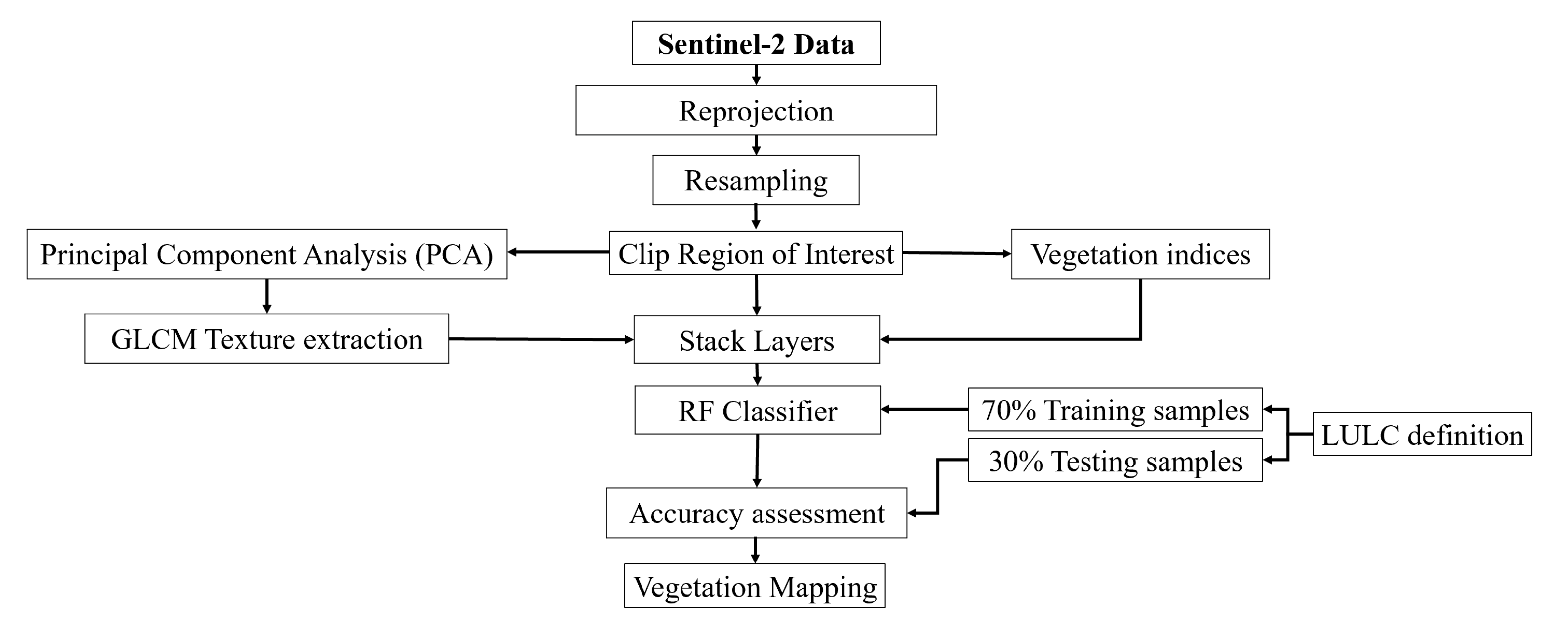
The S2A image processing procedures are synthetically represented in the workflow (Figure 2). Several processing stages were needed to achieve the vegetation mapping.

2.2.1. Dataset and Preprocessing

Sentinel-2A MSI Level-2A images taken on July 18th, 2020, were derived from the Sentinels Scientific Data Hub for the study area (https://scihub.copernicus.eu/, accessed on 29 November 2021). The image was taken during the dry season to ensure a lower cloud coverage percentage (0.25%). The image was projected from WGS84 Geographic latitude/longitude coordinates to EPSG:3763—ETRS89/Portugal TM06, which preserves the area measure.
Sentinel-2 is equipped with MultiSpectral Instrument (MSI), which has four 10 m bands (visible and infrared—NIR), six 20 m bands (red-edge vegetation and short-wave infrared—SWRI), and three 60 m bands [12]. It is possible to increase the spatial resolution of all bands to 10 m using the resampling method and downscale the coarse resolution to a fine resolution [12,13,26]. Pixels of 20 m bands were resampled to the pixel size of 10 m with the Nearest Neighbor technique using ArcGIS Pro (version 2.8, ESRI Portugal, Licensed to the University of Coimbra; https://www.esri.com/en-us/arcgis/products/arcgis-pro/overview, accessed on 29 November 2021).
The high spectral resolution of Sentinel-2 imagery enables the extraction of different features. Based on the literature review and the sensitivity of optical features to biomass, four common spectral vegetation indices (VIs) were derived, namely, Normalized Difference Vegetation Index (NDVI), Green Normalized Difference Vegetation Index (GNDVI), Enhanced Vegetation Index (EVI), and Soil Adjusted Vegetation Index (SAVI), using ArcGIS Pro [27,28]. The complete list of formulas can be found in Table 1 (B2, B3, B4, and B8 are the correspondence S2A bands). NDVI is strongly related to vegetation content, and high NDVI values indicate denser and healthier vegetation. GNDVI is a modified form of NDVI that can detect varying chlorophyll concentration rates by using green reflectance instead of red reflectance [29]. EVI was developed to increase the sensitivity of vegetation signals in high biomass locations [30]. SAVI is also a vegetation index that aims to reduce the impact of soil luminance, particularly in areas with low vegetation cover [31].
In addition to VIs, the previous research proves that using textural features significantly improves classification accuracy, especially for the species with similar spectral characteristics but different spatial patterns [35]. PCA is commonly used in data mining to explore data and reduce data dimensionality [36,37]. It reduces dimensionality by identifying a new set of variables that is smaller than the original set, and captures large principal variability in data while disregarding minor variability [37]. The three first PCs (PC1, PC2, and PC3) having cumulative eigenvalues of more than 99% were extracted from the spectral bands in ArcGIS Pro, as shown in Appendix A (Table A1).
A total of four textural variables, namely, mean (ME), entropy (EN), homogeneity (HO, also called inverse difference moment—IDM), and correlation (CO), were derived using the first three PCs [38]. These textures were obtained through the Gray-Level Co-Occurrence Matrix (GLCM) statistical approach with a probabilistic quantizer (quantization levels of 32), inter-pixel distance of 1, and window size of 5 × 5 using SNAP (version 8.0.0). The window size was optimized based on this particular study area since the texture measures depend on the window size [39]. The formulas of textures and their application are listed in Table 2. The GLCM method examines the distribution of gray levels across adjacent pixels by considering the pixels’ spatial position in an image [40,41,42]. Humeau-Heurtier [40] defined the GLCM P(i,j|d,θ) as a relative frequency of the occurrence of the same intensity value i (reference pixel) adjacent to a different intensity value j (neighbor pixel) in a specific spatial relation at the distance d and direction of θ. Based on these parameters, ME uses the frequency of occurrence of a certain neighboring pixel to weight the pixel value [43]. EN assesses the degree of disorder and complexity of the texture distribution in GLCM [40,42]. HO shows the level of homogeneity [40], and CO measures the linear relationship between pixel values for the grayscale in the horizontal or vertical direction [40,42].

2.2.2. Reference Data

Training samples for each ground object must be selected separately since RF is a supervised classifier. The basis for the selection of training and validation samples was acquired visually from the land use and occupation map (COS2018) of Portugal Directorate-General for the Territory (DGT; Direção-Geral do Território) [47], National Forest Inventory (IFN; Inventário Florestal Nacional) of Portugal Institute for Nature Conservation and Forests (ICNF; Instituto da Conservação da Natureza e das Florestas) [48], and Google Earth orthophoto maps. The reference data were projected to the study area. Common sample polygons were chosen as a base vegetation cartography by filtering and compared with Google Earth images. Moreover, the different color compositions and VIs of the Sentinel-2 image were used to discriminate the vegetation type. The class definition was generalized with more focus on tree species. Vegetation category was selected and verified through visual inspection based on dominant species, as presented in Table 3, such as Pinus pinaster, Eucalyptus, Castanea, Pinus pinea, Quercus (including Quercus robur, Quercus suber, and Quercus ilex), Acacia, and other land uses, including cropland and agriculture land, shrubland and grassland, and water and barren (area without vegetation including roads and urban area) [24]. Therefore, samples’ polygons were manually created based on visual interpretation and reference sources.

2.2.3. Image Classification

A total of 26 independent variables (including ten spectral bands, four vegetation indices, and 12 texture measures) were used as an input to supervised classification to improve the classification performance [8]. The RF algorithm was applied as a machine learning algorithm for vegetation classification in RStudio (version 2022.02.3+492, Rstudio Team, Integrated development environment for R, PBC, Boston, MA, USA; http://www.rstudio.com/, accessed on 29 November 2021). The RF algorithm, an ensemble classifier that produces multiple decision trees, is commonly used in LULC because it yields high accuracy results, solves highly non-linear problems on relatively small-size databases, and handles a large number of input features [49,50,51]. Furthermore, RF enables input feature ranking through random permutation, which has been studied in this paper using the RandomForest package in R [26]. The number of trees (ntree) and the number of random samples per node (mtry) were 500 and 5, respectively. As shown in Appendix A (Figure A1), by increasing ntree, the out-of-bag (OOB) error decreases and becomes stable at around 200 [44,52]. Researchers showed satisfactory results with the default parameter for the RF classifier, which is ntree of 500 trees [53,54]. In addition, an mtry value that is excessively small or large reduces the individual tree’s prediction ability. The optimum value for mtry is calculated as 1/3 or the square root of the number of input variables [44,54]. In this paper, the optimum mtry was calculated as five through the tuneRF function in R, as shown in Appendix A (Figure A2). Samples were randomly subdivided into 70% for the training of the classification algorithm and 30% to validate the model. Finally, an accuracy assessment of vegetation classification was performed by calculating the confusion matrix.

2.2.4. Accuracy Assessment

Accuracy assessments have traditionally relied on a confusion matrix [55]. The confusion matrix measures OA, PA, UA, and kappa to describe the fitness between the generated classes and the reference data [9,20]. OA is directly correlated to the percentage of the study area that is correctly classified, and kappa also measures the performance of RF [55,56]. OA is a relatively coarse measurement since it does not provide information on class-specific accuracy, while PA and UA, respectively, provide class-specific accuracy on the reference and classified area per class [55]. AO, PA, and UA may consider high precision with accuracy above 79% [57], and kappa greater than 80% represents a high degree of agreement [56].

3. Results

A total of 26,100 pixels were selected for the training and validation samples by visual interpretation using reference sources, including DGT, ICNF, and Google Earth. According to the actual occupied area in [24], Pinus pinaster and Eucalyptus have the most significant number of pixels, and other classes have a similar proportion of the actual occupied area. Samples were divided into 70% (17,394 pixels) as training samples, and 30% (8706 pixels) as validation samples using stratified random sampling in R. Appendix B (Table A2) shows the total of 10 classes for this study.
Accuracy assessment of the classification was evaluated based on the confusion matrix and OA, PA, UA, and kappa metrics. The rows and columns of the confusion matrix shown in Table 4 indicate the map classification and the reference classification, respectively. Diagonal cells of the matrix show the correct classifications, and off-diagonal cells indicate misclassifications. Repetition 10 times was conducted for an unbiased evaluation, and the mean accuracy metrics are presented in Table 4. OA of 90.9% (±1) and kappa of 89% (±1) were achieved for this classification, indicating a high classification accuracy. The lowest and highest PA was obtained for Acacia and water, respectively. The other classes have a high PA of over 90%, except for Quercus, with a PA of 79.5%. In the case of UA, barren has the highest accuracy of 97.1%, while Acacia has the lowest value of 70.1%. The predominant species of Pinus pinaster and Eucalyptus have a high UA and PA of over 90%.
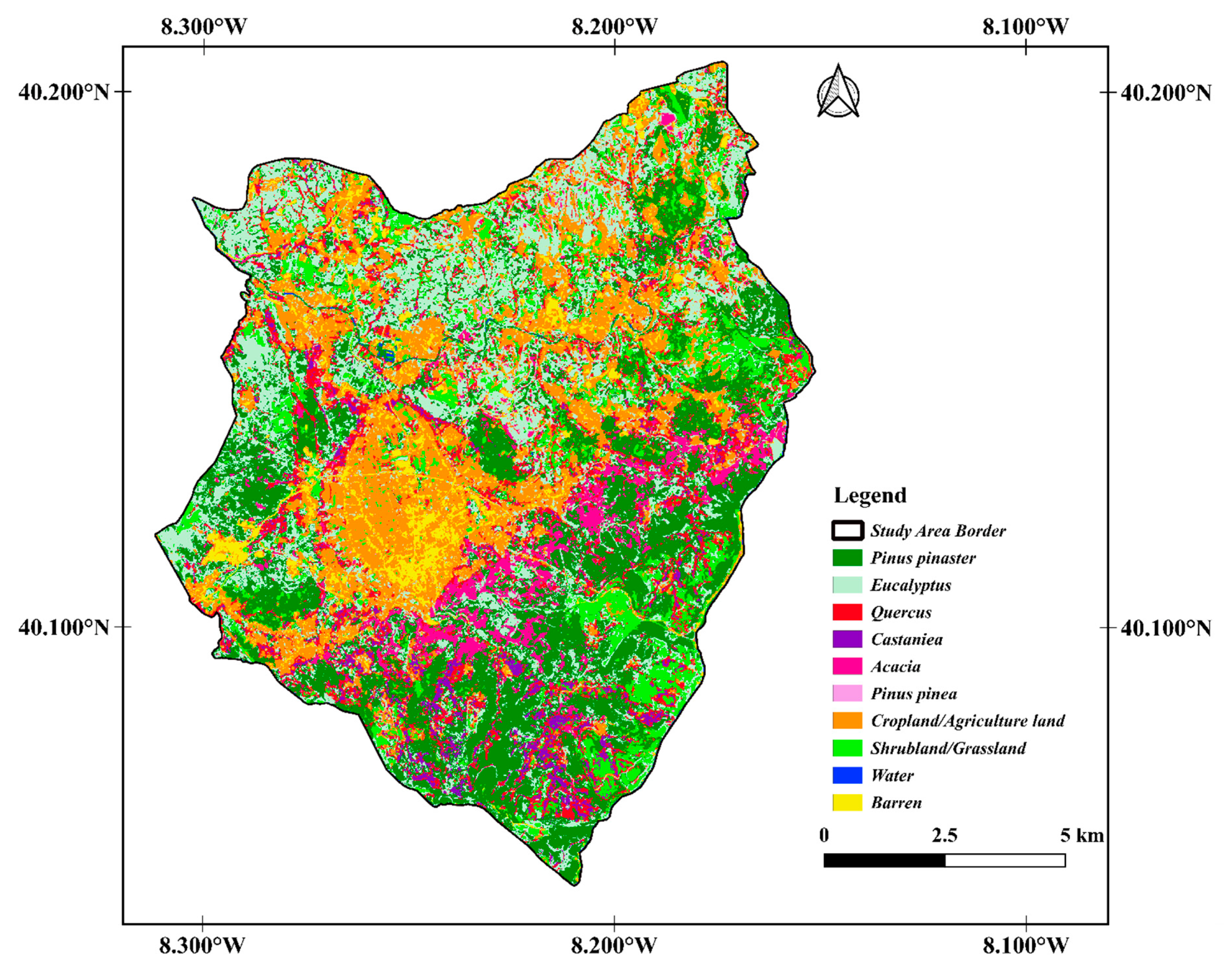
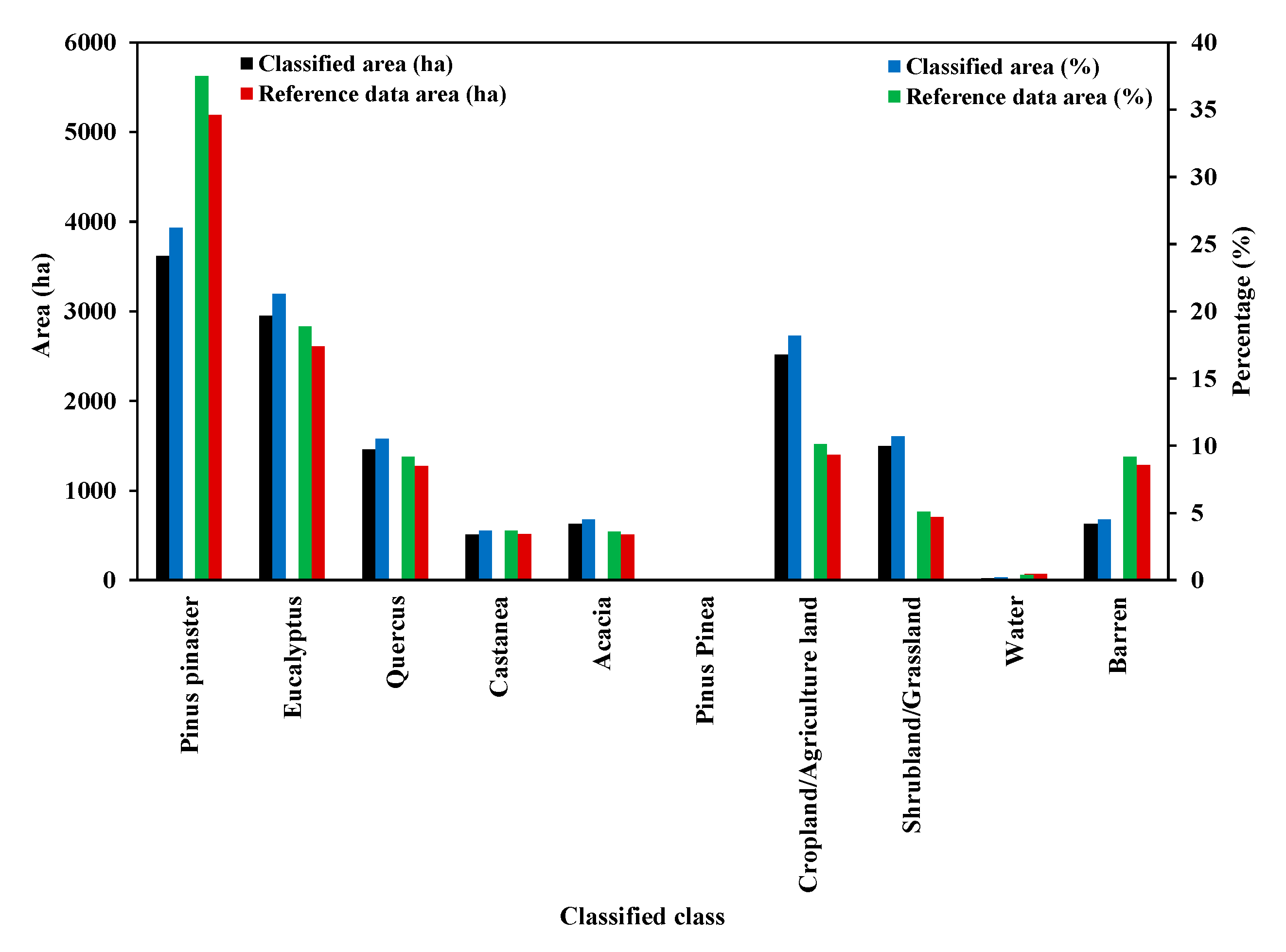
Figure 3 shows the classified vegetation map based on the proposed methodology. Figure 4 represents the area and percentage of each class in the classified map and reference data. The maximum difference in area between classified and reference data was calculated for the Pinus pinaster and Cropland/Agriculture land, with a difference of 11.3% and 8.1%, respectively. According to the result, the largest area is occupied by Pinus pinaster followed by Eucalyptus, mainly in the south and north of the study area, respectively. However, the Pinus pinaster has the majority in the reference data and occupied approximately 37% of the study area [24,47,48]. Since the reference data were based on COS2018 [47], they were not up-to-date and accurate. It is suggested that a field measurement is performed to detect the changes and assess the final classification of this paper. Land cover changes may happen due to natural occurrences such as wildfires, or forestry activities either for commercial purposes by private landowners or forest management. In addition, the study area is very heterogeneous and has several areas with mixed species, making it hard to visually distinguish species using Google Earth images. Moreover, Cropland/Agriculture land class has a greater area than the reference data mentioned in Section 2.1. Some of these misclassifications were due to new plantations and confusion with the Shrubland/Grassland class. Both of these fields have a similar pattern and spectral features of the Cropland/Agriculture land class. The other six classes’ areas predicted similar results compared to the reference data with an error of less than 3%. More information can be found in Appendix B (Table A2). The minimum differences were observed for Castanea and Pinus pinea with a difference of approximately 5 ha (almost zero percent). Errors in testing data may affect the area estimation and amplify bias towards overestimating, especially in rare species in the study area [22].

3.1. Importance of Independent Variables

In order to assess the importance of each variable in RF classification accuracy, mean decrease accuracy (MDA) and mean decrease Gini (Gini) were used through random permutation. Figure 5a,b show the ranking of the variables based on their contribution to distinguishing the classes. This ranking was almost the same for all the repetitions. Band 11 and 12 (SWIR) and band 2 (Blue) have the highest MDA and Gini among the S2A spectral bands, although the NIR band of eight achieved low scores. In the case of the GLCM textures, the ME and CO of PC3 have the highest rank among all 26 variables in MDA. Generally, the ME and CO for the PC1 and PC3 were ranked among the top five variables in both MDA and Gini. Additionally, GNDVI and NDVI have the highest contribution among VIs.
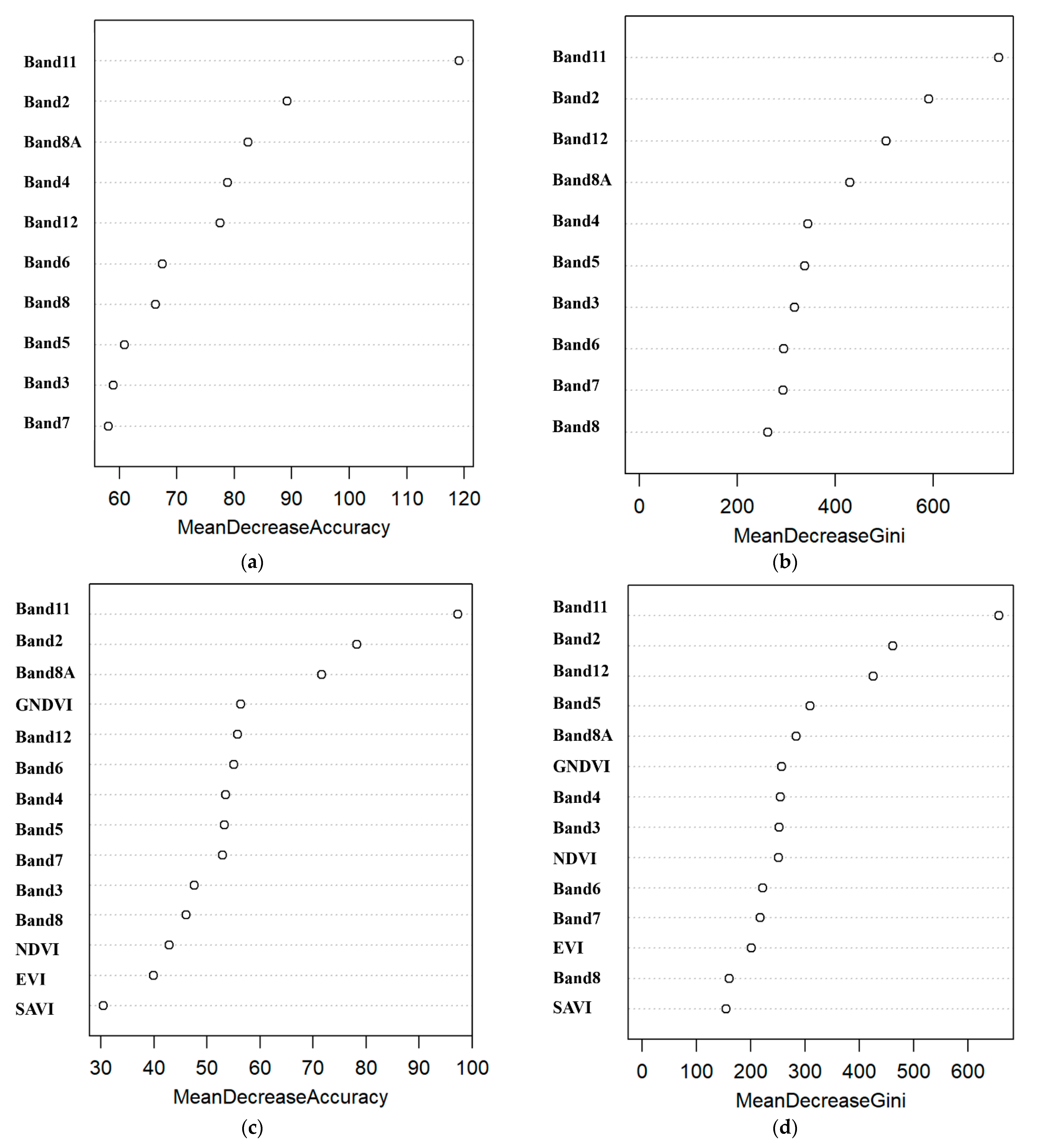
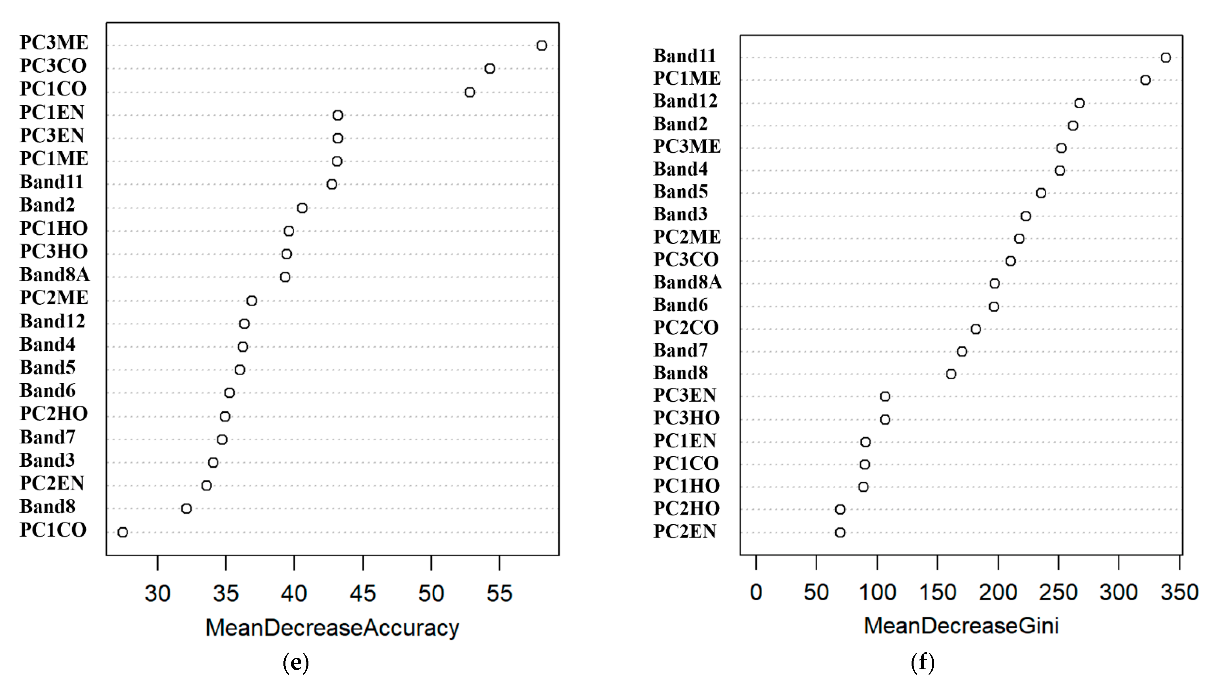
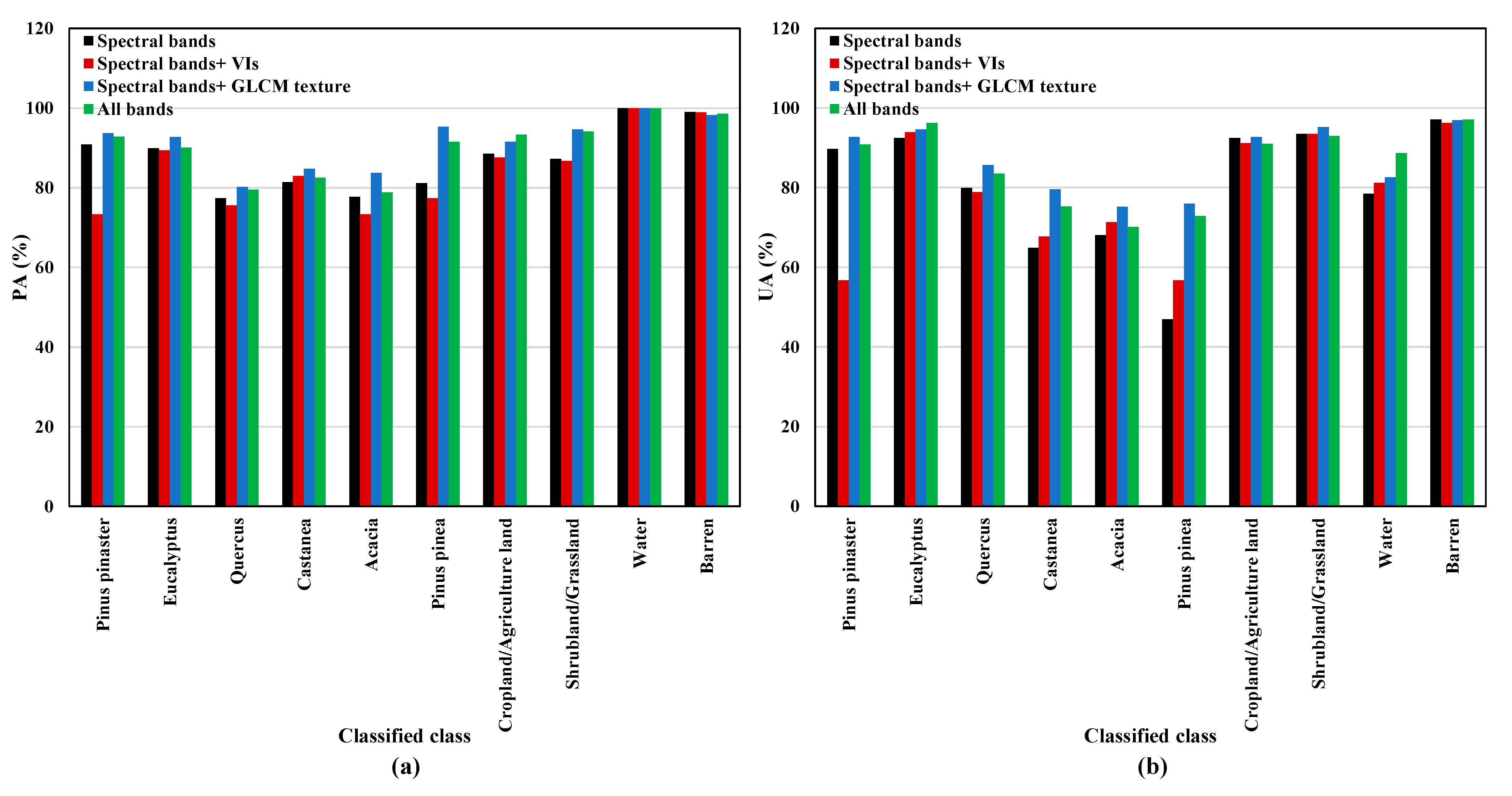
The methodology was applied to different independent variables input to analyze the importance of the GLCM textures. The classification was repeated for three additional scenarios of input bands: (I) only S2A spectral bands, (II) S2A spectral bands and VIs, and (III) S2A spectral bands and GLCM textures. The RF classifier based on the S2A spectral band and GLCM texture achieved the maximum OA and kappa, as presented in Table 5. Using all 26 variables ranked second with a difference of 1.2%, lower than the combination of spectral bands and GLCM textures. The minimum OA and kappa also were obtained for employing only S2A spectral bands. Adding GLCM texture to S2A spectral bands increased the accuracy metrics by 4%. These findings demonstrate the importance of GLCM texture features for improving the predictability of the RF classifier [51]. The inclusion of GLCM textures features affects the OA and enhances class separability. They enable more accurate mapping of vegetation and class discrimination, resulting in improved LCLU classification. According to Costa et al. [22], classified classes′ accuracy determines the maps′ overall accuracy. The RF classifier performance was assessed for four different combinations of input data, shown in Figure 6. An enhancement in PA and UA was observed by adding GLCM texture features. PA and UA for the combination of spectral bands and GLCM texture were higher for most of the classified classes compared to classification without GLCM textures, followed by the combination of all bands. According to feature sets, higher accuracy can be attained by adding more independent variables [26]. However, the combination of spectral bands and GLCM texture were sufficient to achieve high classification accuracy, and adding extra variables does not significantly improve performance [14].
Appendix B (Figure A3) shows the band importance of these three additional classifications. In all of the four scenarios of input variables, band 11 and band 2, ME and CO of PC1 and PC3 outperformed other variables with high values of MDA and Gini. It can be concluded that adding at least one GLCM texture may improve the classification accuracy. In this paper, the ME and CO enhanced the RF classification with higher accuracy.

3.2. Effect of Bootstrap Sample Size

The RF classifier uses bootstrap aggregation, randomly creating different training subsets of the original training dataset to grow the individual regression trees [53,54]. Wang et al. [54] suggested using two-thirds of the validation dataset per subset for the bootstrap sample size. The minimum value of the bootstrap sample size in this paper was equal to the minimum class pixels (water), and the largest sample size was approximately equal to the extraction of highest and lowest class pixels (Pinus pinaster and water). As shown in Figure 7, the lowest and highest OA and kappa were calculated for the sampling size of 137 and 7000, respectively. The highest OA was increased by around 15.7%, and kappa was increased by 19.3%. According to UA and PA, the lowest UA and PA appeared in the sample size of 137 with zero percentage of water and Pinus pinea detection; more information is presented in Appendix B (Table A3). The minimum PA remained below 70% until the sample size of 5000. Thomlinson et al. [58] proposed the minimum OA and per-class accuracy of 85% and 70% for high precision classification, respectively. Although the bootstrap sample size of 6000 and 7000 increased OA and kappa by approximately 1%, the sample size of 5000 was used for this research to avoid overfitting and a highly computational process based on previous studies [26,58]. A bootstrap sample size of 5000 was also equal to two-thirds of the validation dataset in this paper. Furthermore, the lowest and highest OOB errors were obtained for the samples of 5000 and 137, respectively.

4. Discussion

This study achieved high value for the accuracy metrics based on a single image of medium-resolution S2A multispectral bands compared with previous studies that used multi-temporal or high-resolution imagery [17,53]. The main purpose of this study was to increase the interclass separability of forest and vegetation classes and to provide up-to-date data based on S2A for the Lousã region, Portugal.
The LCLU of the study area was divided into ten classes, including the predominant tree species. Sampling data were acquired by visual interpretation of DGT and ICNF data and comparison with Google Earth images (orthophoto maps). The sampling size of this study was approximately 1.3% of the total pixels. The effective sample size is suggested to be between 0.2% to 3% of the total dataset pixels [59]. Increasing the training sample size generally boosts classification accuracy. Many researchers have found a positive correlation between classification accuracy and sample size [21]. According to Moraes et al. [60], there is no recommended minimum sample size, and the sufficient sample size depends on several parameters such as the classifier, predictor variables, class definition, and size and spatial features of the study area. They analyzed the influence of sample size on the LCLU in the north of Portugal using S2 data and the RF classifier. They compared OA for the sample size of 50 to 6000 per class. They found a similar OA value with a variation of 2%, and the highest value of 73.7% indicated the low sensitivity of the RF classifier to the sample size [60].
The classification result had a high OA of 90.9%, although some misclassification was found by comparing the classified map with reference data. The major reasons for different classification statistics may relate to the higher resolution imagery of S2A of 10 m compared with traditional maps, including COS, class definition, and impact of the 2017 wildfire and burnt area on land cover changes [47]. Immitzer et al. [53] mentioned the effect of a parameter such as stand age and density, crown coverage, and understory on the spectral behavior of the tree species and their intra-class separability. Several Pine and Eucalyptus stands were seen in this study area with different ages due to the plantation or cutting. According to Costa et al. [17], spectral confusion between shrubland and tree species or grassland and agricultural land is always expected because of similar spectral features of some classes. They also mentioned the broad conceptual definition of the classes as another factor of misclassification [17]. This paper’s shrubland/grassland class may have a broad conceptual definition since it includes natural, semi-natural, and agricultural grassland and shrubs. Costa et al. [17] also found several classification contradictions between their LCLU classified map and COS2018 [47] for the land cover of mainland Portugal. They presented a significant increase in the occupied area of shrubland and grassland as one of the major land covers of Portugal in comparison with COS [47]. Problematic classes may also result from the fragmented species distribution, either rare or mixed with other classes, especially for tree stands [53]. All these effective factors were considered in this study while comparing the result with the reference data.
As mentioned in Section 3.1, the GLCM texture feature increased the classification accuracy in this study. Several studies have indicated the importance of texture feature extraction in increasing the accuracy of the classified map [26,42,51]. Wang et al. [54] found ME to be the most important variable in mapping forest health conditions using IKONOS imagery. Zhang et al. [42] emphasized the importance of GLCM texture feature extraction on classification accuracy improvement. These textures provide information about different objects with the same spectral, while spectral bands provide the data for the same objects in the different spectra [42]. Zhe et al. [26] suggested using Extended Attribute Profiles (EAPs) in addition to GLCM textures, which can improve shrubland, agricultural land, and barren discrimination. Furthermore, S2A spectral bands have shown a high potential in the LCLU classification of the regional study area of this study without using additional variables, and were also mentioned previously in several research studies [10,26,53]. In this paper, bands 11 (SWIR) and band 2 (blue) were among the five first important variables in all combinations. Immitzer et al. [53] found bands 2 and 11 had the highest score, while the NIR band 8A had the lowest score for forest species classification. Feng et al. [44] declared that spectral features contributed the most in their study with the UAV for flood mapping. In their study, the red and blue bands followed by ME were the most important variables [44]. Wang et al. [54] also achieved high accuracy of 97.1% by using only GLCM feature on IKONOS multispectral bands, which is higher than the accuracy of the combination of all spectral bands and GLCM and Gi (Getis statistic) features (96.9%). They believed that lower accuracy of all bands is associated with increasing omission and commission errors of some Gi features [54]. Wessel et al. [14] found that the application of PCs improved their classification accuracy by 1.8% for the separation of beech and oak trees; however, the addition of NDVI dropped their accuracy by approximately 8%. In this study, vegetation indices may cause lower classification accuracy with all bands. However, the combination of spectral bands and four vegetation indices yielded higher accuracy than only spectral bands and improved the accuracy.
The major limitation of this study is the lack of recent reference data or fieldwork in Portugal. To better analyze the accuracy of the classified map, field measurement data and reliable and up-to-date ground truth data as reference data are needed. Sentinel-2 data are well-suited for forest mapping at tree stand level. However, data fusion or multi-sensor approaches are needed for single tree level classification [14,15]. For future study, the methodology can be extended to mainland Portugal and even some regions of Europe. The results can be validated with fieldwork and fusion of satellite and drone data. The combination of Light Detection and Ranging equipment (LiDAR) data, UAV imagery with finer resolution, Sentinel-1 SAR data, and knowledge of local experts is expected to increase the discrimination of the LCLU classes and provide more information on vertical features of the species. Recently, Portugal has started capturing LiDAR data for the whole country. Nevertheless, it is not yet available for the study area of this paper.

5. Conclusions

This paper proposed a methodology for vegetation mapping by applying a Random Forest classifier to the Sentinel2-A image. Twenty-six independent variables were used by combining ten S2A multispectral bands resampled to a pixel size of 10 m with four vegetation indices and 12 GLCM texture feature variables. These GLCM texture features were calculated from the three first principal components of downscaled S2A spectral bands using PCA. Training and validation data were acquired through forestry data of ICNF and DGT and visual interpretation using Google Earth. An RF classifier with ntree of 500 and mtry of 5 was used to classify the study area into ten classes, including the predominant tree species. A high-precision classification was performed with an overall accuracy of 90.5% and a kappa coefficient of 89%. Nevertheless, employing all 26 variables did not achieve the highest accuracy compared to the combination of spectral bands and GLCM textures, which had an OA of 92%. The comparison of classification accuracy for four different combinations of input variables shows the importance of GLCM textures, especially ME and CO, in improving the performance of the RF classifier. Spectral bands 11 and 2 also have high MDA and Gini scores for all the scenarios. Generally, S2A 10 m spectral bands have strong potential for precise and rapid vegetation classification. GNDVI contributes the most to the accuracy of classification amongst vegetation indices. The results of this study indicate that incorporating at least one GLCM texture feature and at least one vegetation index into the S2A spectral bands can effectively improve the accuracy of assessment and tree species classification.
Few studies have explored highly accurate vegetation mapping in Portugal, particularly in the Lousã region, using Sentinel 2 images. Exploring the multispectral band and texture feature analysis can contribute to the spectral separability of vegetation, facilitating studies of aboveground biomass estimation and wildfire simulation. The accuracy assessment of the implemented methodology showed high potential for generating high-accuracy vegetation mapping over forestry areas. It is expected that the methodology will be expanded to include the fusion of Sentinel 2 and Sentinel 1 data to include data regarding the vertical structure of the vegetation and canopy. These data will enable the creation of a fuel-type tridimensional semantic map to be used by fire behavior models, and allow the definition of biomass management strategies towards wildfire risk reduction or accurate fire spread simulations for the decision support during wildfire events. These results are relevant for the ESA 2025 Agenda, whose challenge is integrating information from Copernicus mapping of carbon to promote sustainable land management and improved resilience against natural risks and impacts of climate change. Therefore, there is a need for more studies to encompass more datasets in Portugal.

Author Contributions

Conceptualization, P.M.; methodology, P.M.; software, P.M.; validation, P.M.; formal analysis, P.M.; investigation, P.M.; resources, P.M.; data curation, P.M.; writing—original draft preparation, P.M.; writing—review and editing, P.M., D.X.V. and C.V.; visualization, P.M.; supervision, D.X.V. and C.V.; project administration, C.V.; funding acquisition, C.V. All authors have read and agreed to the published version of the manuscript.

Funding

This work is financed by national funds through FCT—Foundation for Science and Technology, under grant agreement 2021.05971. BD attributed to the 1st author. The authors gratefully acknowledge the Portuguese Foundation for Science and Technology (FCT) for its support under the framework of the research projects FIREFRONT—RealTime Forest Fire Mapping and Spread Forecast Using Unmanned Aerial Vehicles, ref. PCIF/SSI/0096/2017, and IMFire—Intelligent Management of Wildfires, ref. PCIF/SSI/0151/2018, fully funded by national funds through the Ministry of Science, Technology, and Higher Education and project FirEUrisk—Developing a Holistic, Risk-Wise Strategy for European Wildfire Management, funded by the European Union’s Horizon 2020 research and innovation programme under grant agreement No. 101003890.

Data Availability Statement

The data presented in this study are available on request from the corresponding author.

Acknowledgments

The authors thank the project partner, the University of Coimbra, the University of Alcala, the Portuguese Foundation for Science and Technology (FCT), and the Horizon 2020 research and innovation programme for supporting this work.

Conflicts of Interest

The authors declare no conflict of interest.

Abbreviations

B2S2A band2
B3S2A band3
B4S2A band4
B8S2A band8
NNumber of grey levels
PNormalized symmetric GLCM of dimension N × N
P (i, j)Normalized grey level value in the cell i, j of the co-occurrence matrix
dDistance
θDirection
x ¯ Mean of Px
y ¯ Mean of Py
σ x Standard deviation of Px
σ y Standard deviation of Py

Appendix A

Table A1. Percent and accumulative eigenvalues of three first PCs.
PC LayerPercent of Eigenvalues (%)Accumulative of Eigenvalues (%)
PC192.592.5
PC26.398.8
PC30.699.4
Figure A1. OOB Error of the number of RF mtry.
Remotesensing 14 04585 g0a1
Figure A2. OOB Error of the number of RF mtry.
Remotesensing 14 04585 g0a2

Appendix B

Table A2. Classification result represented in the area (ha) and percentage.
Class IDClassified ClassClassified Area (ha)Percentage (%)The Difference with Reference Data Area (ha)The Difference with Reference Data Area (%)
1Pinus pinaster3619.186726.2−1570.9833−11.3
2Eucalyptus2951.436521.3+339.4865+2.4
3Quercus1453.587010.5−180.227−1.3
4Castanea506.38173.7−4.5483−0.0
5Acacia626.28974.5+120.0297+0.9
6Pinus pinea17.16250.1+5.9825+0.0
7Cropland/Agriculture land2518.388618.2+1119.0689+8.1
8Shrubland/Grassland1499.600810.7+798.0708+5.6
9Water21.92600.2−42.914−0.2
10Barren625.98954.5−655.2805−4.7
Figure A3. Mean decrease accuracy and mean decrease Gini for three different combinations of variables: (I) Spectral bands (a,b), (II) Spectralbands + VIs (c,d), and (III) Spectralbands + GLCM texture (e,f).
Remotesensing 14 04585 g0a3aRemotesensing 14 04585 g0a3b
Table A3. Effect of sample size on OA, UA, PA, and Kappa in RF classification.
Sample Size1371000200030004000500060007000
OA (%)76.585.288.287.889.990.991.692.2
Kappa (%)71.28285.785.187.78989.990.5
Max PA (%)91 Barren95.8 Barren94 Eucalyptus96 Barren96.3 Barren100 water96.7 Barren97.9 Barren
Min PA (%)0 Water & Pinus pinea56.1 Pinus pinea65 Acacia60 Acacia69 Castanea78.8 Acacia75.4 Castanea71.3 Pinus pinea
Max UA (%)91 Barren100 Water100 Water100 Water100 Pinus pinea97.1 Barren100 Water100 Water/Pinuspinea
Min UA (%)0 Water & Pinus pinea66.6 Quercus70 Quercus70 Quercus74.2 Quercus70.1 Acacia80.8 Quercus81.1 Quercus
Lowest OOB Error (%)23.514.8312.110.7108.38.78.4
Optimum mtry101051010555
ntreeNot stableStableStableStableStableStableStableStable

References

  1. Xavier, A.C.; Rudorff, B.F.T.; Shimabukuro, Y.E.; Berka, L.M.S.; Moreira, M.A. Multi-temporal analysis of MODIS data to classify sugarcane crop. Int. J. Remote Sens. 2006, 27, 755–768. [Google Scholar] [CrossRef]
  2. World Bank. Investment in Disaster Risk Management in Europe Makes Economic Sense; World Bank: Washington, DC, USA, 2021. [Google Scholar] [CrossRef]
  3. Costa, H.; de Rigo, D.; Libertà, G.; Houston Durrant, T.; San-Miguel-Ayanz, J. European Wildfire Danger and Vulnerability in a Changing Climate: Towards Integrating Risk Dimensions; Publications Office of the European Union: Mercier, Luxembourg, 2020. [Google Scholar] [CrossRef]
  4. Benali, A.; Fernandes, P. Understanding the impact of different landscape-level fuel management strategies on wildfire hazard Understanding the impact of different landscape-level fuel management strategies on wildfire hazard. Forests 2021, 12, 522. [Google Scholar] [CrossRef]
  5. Monteiro-Henriques, T.; Fernandes, P.M. Regeneration of native forest species in Mainland Portugal: Identifying main drivers. Forests 2018, 9, 694. [Google Scholar] [CrossRef]
  6. Instituto Português do Mar e da Atmosfera (IPMA) May Climatological Bulletin. Available online: https://www.ipma.pt/pt/media/noticias/news.detail.jsp?f=/pt/media/noticias/textos/Boletim_climatologico_maio.html (accessed on 15 June 2022).
  7. Kolström, M.; Vile, T.; Lindner, M. Climate Change Impacts and Adaptation in European Forests. EFI Policy Brief 2011, 6, 14. [Google Scholar]
  8. Aragoneses, E.; Chuvieco, E. Generation and mapping of fuel types for fire risk assessment. Fire 2021, 4, 59. [Google Scholar] [CrossRef]
  9. Xie, Y.; Sha, Z.; Yu, M. Remote sensing imagery in vegetation mapping: A review. J. Plant Ecol. 2008, 1, 9–23. [Google Scholar] [CrossRef]
  10. Chaves, M.E.D.; Picoli, M.C.A.; Sanches, I.D. Recent applications of Landsat 8/OLI and Sentinel-2/MSI for land use and land cover mapping: A systematic review. Remote Sens. 2020, 12, 3062. [Google Scholar] [CrossRef]
  11. Zeng, L.; Wardlow, B.D.; Xiang, D.; Hu, S.; Li, D. A review of vegetation phenological metrics extraction using time-series, multispectral satellite data. Remote Sens. Environ. 2020, 237, 111511. [Google Scholar] [CrossRef]
  12. Kaplan, G. Broad-Leaved and Coniferous Forest Classification in Google Earth Engine Using Sentinel Imagery. Environ. Sci. Proc. 2021, 3, 64. [Google Scholar] [CrossRef]
  13. ESA. Sentinel-2 User Handbook. 2015. Available online: https://sentinel.esa.int/documents/247904/685211/Sentinel-2_User_Handbook (accessed on 10 November 2021).
  14. Wessel, M.; Brandmeier, M.; Tiede, D. Evaluation of different machine learning algorithms for scalable classification of tree types and tree species based on Sentinel-2 data. Remote Sens. 2018, 10, 1419. [Google Scholar] [CrossRef]
  15. Fassnacht, F.E.; Latifi, H.; Stereńczak, K.; Modzelewska, A.; Lefsky, M.; Waser, L.T.; Straub, C.; Ghosh, A. Review of studies on tree species classification from remotely sensed data. Remote Sens. Environ. 2016, 186, 64–87. [Google Scholar] [CrossRef]
  16. Hernandez, I.; Benevides, P.; Costa, H.; Caetano, M. Exploring sentinel-2 for land cover and crop mapping in portugal. Int. Arch. Photogramm. Remote Sens. Spat. Inf. Sci.—ISPRS Arch. 2020, 43, 83–89. [Google Scholar] [CrossRef]
  17. Costa, H.; Benevides, P.; Moreira, F.D.; Moraes, D.; Caetano, M. Spatially Stratified and Multi-Stage Approach for National Land Cover Mapping Based on Sentinel-2 Data and Expert Knowledge. Remote Sens. 2022, 14, 1865. [Google Scholar] [CrossRef]
  18. Persson, M.; Lindberg, E.; Reese, H. Tree species classification with multi-temporal Sentinel-2 data. Remote Sens. 2018, 10, 1794. [Google Scholar] [CrossRef]
  19. Pacheco, A.D.P.; Junior, J.A.D.S.; Ruiz-Armenteros, A.M.; Henriques, R.F.F. Assessment of k-nearest neighbor and random forest classifiers for mapping forest fire areas in central portugal using landsat-8, sentinel-2, and terra imagery. Remote Sens. 2021, 13, 1345. [Google Scholar] [CrossRef]
  20. Sheykhmousa, M.; Mahdianpari, M.; Ghanbari, H.; Mohammadimanesh, F.; Ghamisi, P.; Homayouni, S. Support Vector Machine Versus Random Forest for Remote Sensing Image Classification: A Meta-Analysis and Systematic Review. IEEE J. Sel. Top. Appl. Earth Obs. Remote Sens. 2020, 13, 6308–6325. [Google Scholar] [CrossRef]
  21. Ma, L.; Li, M.; Ma, X.; Cheng, L.; Du, P.; Liu, Y. A review of supervised object-based land-cover image classification. ISPRS J. Photogramm. Remote Sens. 2017, 130, 277–293. [Google Scholar] [CrossRef]
  22. Costa, H.; Almeida, D.; Vala, F.; Marcelino, F.; Caetano, M. Land cover mapping from remotely sensed and auxiliary data for harmonized official statistics. ISPRS Int. J. Geo-Inf. 2018, 7, 157. [Google Scholar] [CrossRef]
  23. Liu, H.; Gong, P.; Wang, J.; Wang, X.; Ning, G.; Xu, B. Production of global daily seamless data cubes and quantification of global land cover change from 1985 to 2020—iMap World 1.0. Remote Sens. Environ. 2021, 258, 112364. [Google Scholar] [CrossRef]
  24. Incêndios, C.; Base, I.; Florestal, G.T. Plano Municipal de Defesa da Floresta Contra Incêndios; Município de Vila Nova de Poiares: Vila Nova de Poiares, Portugal, 2020. [Google Scholar]
  25. Viegas, D.X.; Figueiredo Almeida, M.; Ribeiro, L.M.; Raposo, J.; Viegas, M.T.; Oliveira, R.; Alves, D.; Pinto, C.; Jorge, H.; Rodrigues, A.; et al. O Complexo de Incêndios de Pedrogão Grande E Concelhos Limítrofes, Iniciado a 17 de Junho de 2017. Iniciado A 2017, 2017, 238. [Google Scholar]
  26. Zheng, H.; Du, P.; Chen, J.; Xia, J.; Li, E.; Xu, Z.; Li, X.; Yokoya, N. Performance evaluation of downscaling sentinel-2 imagery for Land Use and Land Cover classification by spectral-spatial features. Remote Sens. 2017, 9, 1274. [Google Scholar] [CrossRef]
  27. Noi Phan, T.; Kuch, V.; Lehnert, L.W. Land cover classification using google earth engine and random forest classifier-the role of image composition. Remote Sens. 2020, 12, 2411. [Google Scholar] [CrossRef]
  28. Xia, H.; Zhao, W.; Li, A.; Bian, J.; Zhang, Z. Subpixel inundation mapping using landsat-8 OLI and UAV data for a wetland region on the zoige plateau, China. Remote Sens. 2017, 9, 31. [Google Scholar] [CrossRef]
  29. Gitelson, A.A.; Kaufman, Y.J.; Merzlyak, M.N. Use of a green channel in remote sensing of global vegetation from EOS—MODIS. Remote Sens. Environ. 1996, 58, 289–298. [Google Scholar] [CrossRef]
  30. Bhatnagar, S.; Gill, L.; Regan, S.; Waldren, S.; Ghosh, B. A nested drone-satellite approach to monitoring the ecological conditions of wetlands. ISPRS J. Photogramm. Remote Sens. 2021, 174, 151–165. [Google Scholar] [CrossRef]
  31. Somvanshi, S.S.; Kumari, M. Comparative analysis of different vegetation indices with respect to atmospheric particulate pollution using sentinel data. Appl. Comput. Geosci. 2020, 7, 100032. [Google Scholar] [CrossRef]
  32. Agarwal, A.; Kumar, S.; Singh, D. Development of neural network based adaptive change detection technique for land terrain monitoring with satellite and drone images. Def. Sci. J. 2019, 69, 474–480. [Google Scholar] [CrossRef]
  33. Gitelson, A.; Merzlyak, M.N. Quantitative estimation of chlorophyll-a using reflectance spectra: Experiments with autumn chestnut and maple leaves. J. Photochem. Photobiol. B 1994, 22, 247–252. [Google Scholar] [CrossRef]
  34. Alam, M.J.; Rahman, K.M.; Asna, S.M.; Muazzam, N.; Ahmed, I.; Chowdhury, M.Z. Comparative studies on IFAT, ELISA & DAT for serodiagnosis of visceral leishmaniasis in Bangladesh. Bangladesh Med. Res. Counc. Bull. 1996, 22, 27–32. [Google Scholar]
  35. Gini, R.; Sona, G.; Ronchetti, G.; Passoni, D.; Pinto, L. Improving tree species classification using UAS multispectral images and texture measures. ISPRS Int. J. Geo-Inf. 2018, 7, 315. [Google Scholar] [CrossRef]
  36. Guo, Q.; Wu, W.; Massart, D.L.; Boucon, C.; De Jong, S. Feature selection in principal component analysis of analytical data. Chemom. Intell. Lab. Syst. 2002, 61, 123–132. [Google Scholar] [CrossRef]
  37. Xiao, B. Principal component analysis for feature extraction of image sequence. In Proceedings of the 2010 International Conference on Computer and Communication Technologies in Agriculture Engineering, Chengdu, China, 12–13 June 2010. [Google Scholar]
  38. Kattenborn, T.; Lopatin, J.; Förster, M.; Christian, A.; Ewald, F. Remote Sensing of Environment UAV data as alternative to fi eld sampling to map woody invasive species based on combined Sentinel-1 and Sentinel-2 data. Remote Sens. Environ. 2019, 227, 61–73. [Google Scholar] [CrossRef]
  39. Chatziantoniou, A.; Petropoulos, G.P.; Psomiadis, E. Co-Orbital Sentinel 1 and 2 for LULC mapping with emphasis on wetlands in a mediterranean setting based on machine learning. Remote Sens. 2017, 9, 1259. [Google Scholar] [CrossRef]
  40. Humeau-Heurtier, A. Texture feature extraction methods: A survey. IEEE Access 2019, 7, 8975–9000. [Google Scholar] [CrossRef]
  41. Xu, J.L.; Gowen, A.A. Spatial-spectral analysis method using texture features combined with PCA for information extraction in hyperspectral images. J. Chemom. 2020, 34, e3132. [Google Scholar] [CrossRef]
  42. Zhang, X.; Cui, J.; Wang, W.; Lin, C. A study for texture feature extraction of high-resolution satellite images based on a direction measure and gray level co-occurrence matrix fusion algorithm. Sensors 2017, 17, 1474. [Google Scholar] [CrossRef]
  43. Held, M.; Committee, T.I.B. GLCM texture: A tutorial. In Proceedings of the 17th International Symposium on Ballistics, Midrand, South Africa, 23–27 March 1998; Volume 2, pp. 267–274. [Google Scholar]
  44. Feng, Q.; Liu, J.; Gong, J. Urban flood mapping based on unmanned aerial vehicle remote sensing and random forest classifier-A case of yuyao, China. Water 2015, 7, 1437–1455. [Google Scholar] [CrossRef]
  45. Nizalapur, V.; Vyas, A. Texture analysis for land use land cover (LULC) classification in parts of Ahmedabad, Gujarat. Int. Arch. Photogramm. Remote Sens. Spat. Inf. Sci.—ISPRS Arch. 2020, 43, 275–279. [Google Scholar] [CrossRef]
  46. Haralick, R.M.; Shanmugam, K.; Dinstein, I. Textural Features for Image Classification. SEG Tech. Program Expand. Abstr. 1973, 3, 610–621. [Google Scholar] [CrossRef]
  47. Portugal Directorate-General for the Territory (DGT)-Carta de Uso e Ocupação do Solo de Portugal Continental (COS2018). Available online: https://www.dgterritorio.gov.pt/Carta-de-Uso-e-Ocupacao-do-Solo-para-2018 (accessed on 10 December 2021).
  48. ICNF 6º Inventário Florestal Nacional (IFN6; 2015)- Relatório Final. Instituto da Conservação da Natureza e das Florestas Lisboa, Portugal. Available online: https://geocatalogo.icnf.pt/catalogo_tema3.html (accessed on 10 December 2021).
  49. Kluczek, M.; Zagajewski, B. Airborne HySpex Hyperspectral Versus Multitemporal Sentinel-2 Images for Mountain Plant Communities Mapping. Remote Sens. 2022, 14, 1209. [Google Scholar] [CrossRef]
  50. Wójtowicz, A.; Piekarczyk, J.; Czernecki, B.; Ratajkiewicz, H. A random forest model for the classification of wheat and rye leaf rust symptoms based on pure spectra at leaf scale. J. Photochem. Photobiol. B 2021, 223, 112278. [Google Scholar] [CrossRef] [PubMed]
  51. Adeli, S.; Quackenbush, L.J.; Salehi, B.; Mahdianpari, M. The Importance of Seasonal Textural Features for Object-Based Classification of Wetlands: New York State Case Study. Int. Arch. Photogramm. Remote Sens. Spat. Inf. Sci. 2022, 43, 471–477. [Google Scholar] [CrossRef]
  52. Hanes, C.C.; Wotton, M.; Woolford, D.G.; Martell, D.L.; Flannigan, M. Mapping organic layer thickness and fuel load of the boreal forest in Alberta, Canada. Geoderma 2022, 417, 115827. [Google Scholar] [CrossRef]
  53. Immitzer, M.; Vuolo, F.; Atzberger, C. First experience with Sentinel-2 data for crop and tree species classifications in central Europe. Remote Sens. 2016, 8, 166. [Google Scholar] [CrossRef]
  54. Wang, H.; Zhao, Y.; Pu, R.; Zhang, Z. Mapping Robinia pseudoacacia forest health conditions by using combined spectral, spatial, and textural information extracted from IKONOS imagery and random forest classifier. Remote Sens. 2015, 7, 9020–9044. [Google Scholar] [CrossRef]
  55. Stehman, S.V.; Foody, G.M. Key issues in rigorous accuracy assessment of land cover products. Remote Sens. Environ. 2019, 231, 111199. [Google Scholar] [CrossRef]
  56. Landis, J.R.; Koch, G.G. The Measurement of Observer Agreement for Categorical Data. Biometrics 1977, 33, 159–174. [Google Scholar] [CrossRef]
  57. Story, M.; Congalton, R.G. Remote Sensing Brief Accuracy Assessment: A User’s Perspective. Photogramm. Eng. Remote Sens. 1986, 52, 397–399. [Google Scholar]
  58. Thomlinson, J.R.; Bolstad, P.V.; Cohen, W.B. Coordinating methodologies for scaling landcover classifications from site-specific to global: Steps toward validating global map products. Remote Sens. Environ. 1999, 70, 16–28. [Google Scholar] [CrossRef]
  59. Blatchford, M.L.; Mannaerts, C.M.; Zeng, Y. Determining representative sample size for validation of continuous, large continental remote sensing data. Int. J. Appl. Earth Obs. Geoinf. 2021, 94, 102235. [Google Scholar] [CrossRef]
  60. Moraes, D.; Benevides, P.; Costa, H.; Moreira, F.D.; Caetano, M. Influence of Sample Size in Land Cover Classification Accuracy Using Random Forest and Sentinel-2 Data in Portugal. In Proceedings of the 2021 IEEE International Geoscience and Remote Sensing Symposium IGARSS, Brussels, Belgium, 11–16 July 2021. [Google Scholar]
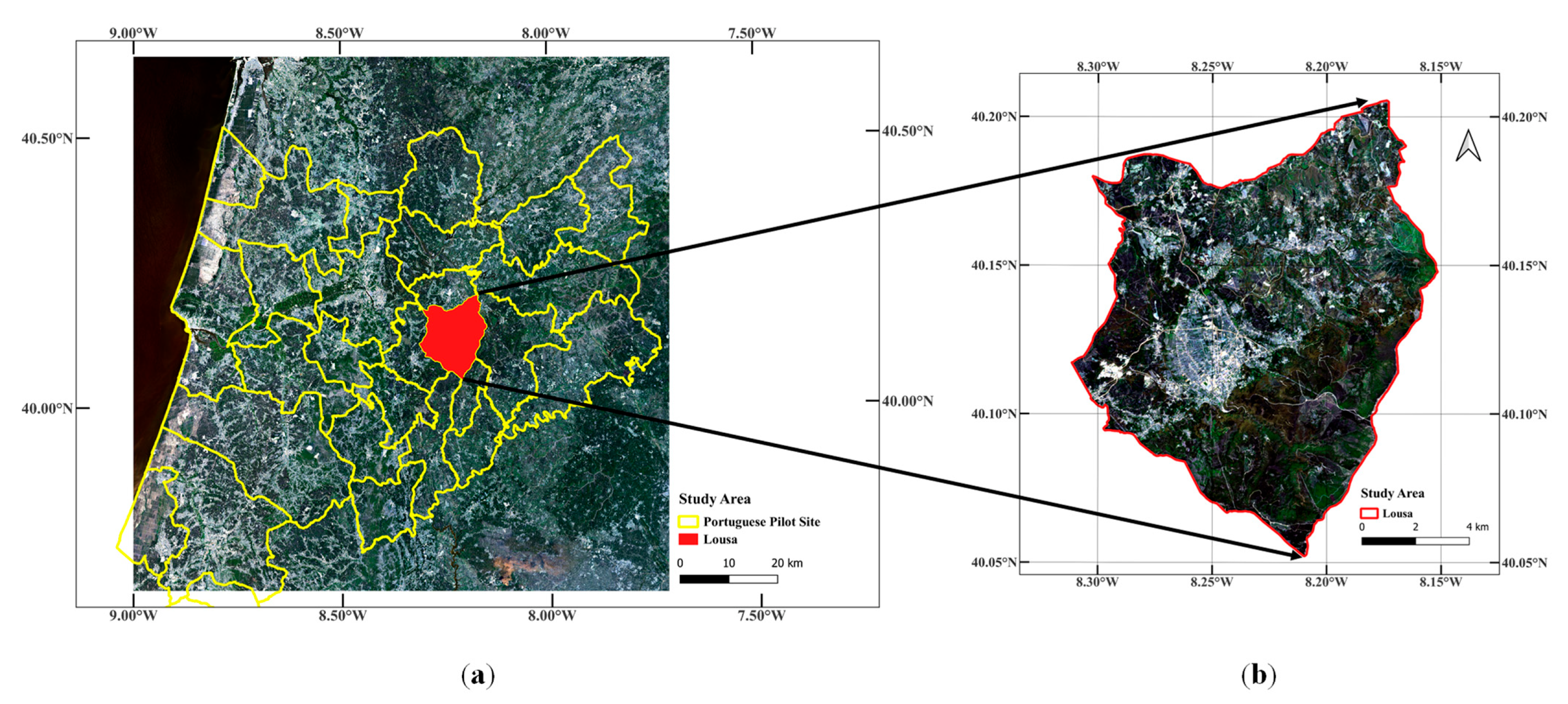
Figure 1. Geographical framework of the location and limits of the study area within a FirEUrisk project and mainland Portugal: (a) Sentinel-2 false-color composite image; (b) study area—Lousã.
Remotesensing 14 04585 g001
Figure 2. Scheme of vegetation mapping with Sentinel-2 data.
Remotesensing 14 04585 g002
Figure 3. Vegetation map generated based on 26 independent variables of S2A imagery using RF classification for Lousã, Portugal.
Remotesensing 14 04585 g003
Figure 4. Comparison of classification result and reference data represented in total area (ha) and percentage of the whole study area.
Remotesensing 14 04585 g004
Figure 5. Band importance ranking based on: (a) mean decrease accuracy and (b) mean decrease Gini.
Remotesensing 14 04585 g005
Figure 6. Class accuracy for different combinations of independent variables: (a) producer accuracy and (b) user accuracy.
Remotesensing 14 04585 g006
Figure 7. Effect of sample size on OA, UA, PA, kappa, and OOB error in RF classification.
Remotesensing 14 04585 g007
Table 1. Vegetation indices (VIs) and applications from S2A.
Vegetation IndicesFormulationApplication
NDVI B 8 B 4 B 8 + B 4 Detection of vegetation communities in various seasons [30]
Estimating changes in vegetation state [29]
Determining the density of greenness [32]
GNDVI B 8 B 3 B 8 + B 3 Determining water and nitrogen uptake in the crop canopy [29,33]
EVI B 8 B 4 B 8 + 6 × B 4 7.5 × B 2 + 1 × 2.5 Detection of vegetation communities in various seasons [30]
Land cover classification [27]
SAVI B 8 B 4 B 8 + B 4 + 0.5 × 1.5 Minimizing soil brightness influences [31,34]
Land cover classification [27]
Table 2. Texture metrics formulas.
Texture MetricsFormulationApplication
ME i N j N i × P i , j | d , θ Weighting pixel value based on the frequency of its occurrence in conjunction with a specific neighbor pixel value [43,44]
Calculating the mean processing window value [45]
EN i N j N P i , j | d , θ log 2 P i , j | d , θ Assessing the disorder of the GLCM [40]
Reflecting the complexity of the texture distribution [42]
HO i N j N P i , j | d , θ 1 + i j 2 Measuring the level of homogeneity in pairs of pixels [40]
CO i N j N i x ¯ j y ¯ P i , j | d , θ σ x σ y Measuring grey level linear relation between pixels [40,42,46]
Table 3. Dominant species represented in ha and percentage adapted from [24].
SpeciesArea (ha)Percentage of the Study Area (%)
Pinus pinaster5190.1737.5
Eucalyptus2611.9518.9
Quercus1273.369.2
Castanea510.933.7
Acacia506.263.6
Pinus pinea11.180.1
Table 4. Confusion matrix and statistical measures for RF vegetation classification.
ReferenceTotalPA
ClassificationClasses 12345678910N° Pixels%
1Pinus pinaster21364036186300540230292.8
2Eucalyptus10120521311411265117227790.1
3Quercus3210580647017200073079.5
4Castanea2424133310010040282.5
5Acacia302691760000022378.8
6Pinus pinea000004303014791.5
7Cropland/Agriculture land1055602638101768493.3
8Shrubland/Grassland19211310311108300115194.1
9Water0000000039039100
10Barren02100090083184398.6
TotalN° Pixels23522134695442251597011164448568706
UA%90.896.283.575.370.172.9919388.697.1
OA90.9%
K89%
Table 5. OA and kappa for RF classification with different combinations of independent variables.
All BandsSpectral BandsSpectral Bands + VisSpectral Bands + GLCM Texture
OA (%)90.88888.692
Kappa (%)898686.190.2
Publisher’s Note: MDPI stays neutral with regard to jurisdictional claims in published maps and institutional affiliations.