Article

The Influence of Satellite-Derived Environmental and Oceanographic Parameters on Marine Turtle Time at Surface in the Gulf of Mexico

1
Cherokee Nation Technologies, Contracted to U.S. Geological Survey Wetland and Aquatic Research Center, Davie, FL 33314, USA
2
Department of Oceanography and Coastal Sciences, Louisiana State University, Baton Rouge, LA 70803, USA
3
National Oceanic and Atmospheric Administration Southeast Fisheries Science Center, Miami, FL 33149, USA
4
Cooperative Institute for Marine and Atmospheric Studies, University of Miami, Miami, FL 33149, USA
5
College of Marine Science, University of South Florida, St. Petersburg, FL 33701, USA
6
U.S. Geological Survey, Wetland and Aquatic Research Center, Gainesville, FL 32653, USA
7
U.S. Geological Survey, Wetland and Aquatic Research Center, Davie, FL 33314, USA
*
Author to whom correspondence should be addressed.
Remote Sens. 2022, 14(18), 4534; https://doi.org/10.3390/rs14184534
Submission received: 24 August 2022 / Revised: 7 September 2022 / Accepted: 9 September 2022 / Published: 11 September 2022
(This article belongs to the Special Issue Remote Sensing Applications for Sea Turtle Conservation)

Abstract

:
The aftermath of the 2010 Deepwater Horizon oil spill highlighted the lack of baseline spatial, behavioral, and abundance data for many species, including imperiled marine turtles, across the Gulf of Mexico. The ecology of marine turtles is closely tied to their vertical movements within the water column and is therefore critical knowledge for resource management in a changing ocean. A more comprehensive understanding of diving behavior, specifically surface intervals, can improve the accuracy of density and abundance estimates by mitigating availability bias. Here, we focus on the proportion of time marine turtles spend at the top 2 m of the water column to coincide with depths where turtles are assumed visible to observers during aerial surveys. To better understand what environmental and oceanographic conditions influence time at surface, we analyzed dive and spatial data from 136 satellite tags attached to three species of threatened or endangered marine turtles across 10 years. We fit generalized additive models with 11 remotely sensed covariates, including sea surface temperature (SST), bathymetry, and salinity, to examine dive patterns. Additionally, the developed model is the first to explicitly examine the potential connection between turtle dive patterns and ocean frontal zones in the Gulf of Mexico. Our results show species-specific associations of environmental covariates related to increased time at surface, particularly for depth, salinity, and frontal features. We define seasonal and spatial variation in time-at-surface patterns in an effort to contribute to marine turtle density and abundance estimates. These estimates could then be utilized to generate correction factors for turtle detection availability during aerial surveys.

1. Introduction

Rapid environmental change is affecting species distributions at an unprecedented pace, which could in turn affect ecosystem function and resilience [1]. Such climate-related shifts can have significant and potentially detrimental implications for migratory species such as birds, mammals, and marine turtles that move seasonally between foraging and breeding areas [2,3]. Understanding how this wide-ranging movement is influenced by biotic and abiotic factors is a key element in contemporary species distribution modeling and, by extension, management frameworks that address migratory species [2,4]. Incorporating migratory species into spatial management frameworks, such as marine protected areas or fisheries closures, presents a unique conservation challenge, yet such measures are necessary to combat rapid, global population declines in marine species [5,6].
Studies that spatially link animal movement to environmental drivers are ubiquitous in the literature (e.g., [7,8]). However, the relationship between many oceanographic conditions and diving patterns or behavior is still poorly understood [9,10]. Recent technological advances in data loggers and remote sensors now allow for detailed observations of animal use of the water column at a scale relevant for marine management and further biogeographic studies [11,12,13]. There is significant spatiotemporal variation in dive behavior and even more so when the physiological constraints of the individual animal (i.e., age, body mass, etc.) are considered. Diving behavior for many marine species is thought to primarily occur in tandem with foraging [10,14], although dives can also occur to escape predators or locate cooler water temperatures [9,15]. An improved understanding of dive patterns enables complex investigation into how animals search for and capture prey, detailed energetic and activity budgets, and habitat use [14,16].
Measurements of dive behavior are increasingly being tested and modeled for environmental associations. For example, numerous studies have utilized satellite-derived sea surface temperature to correlate dives with foraging behavior in elephant seals [17], marine turtles [12], and whale sharks [18]. Additional environmental variables considered to influence dive patterns have included bathymetry, salinity, ocean productivity, or other physiographic features (i.e., continental shelf) [15,19]. The development of models that relate biologging data (i.e., animal distribution or activity data loggers) to environmental parameters require biological data at the appropriate sample size as well as sufficient geographic and temporal representation. Often, the necessary data are either unmeasured or not available at the appropriate scale and proxies such as space (latitude/longitude) and time (month/year) are integrated into the modeling framework, potentially limiting the interpretability of the model output [20]. The increased availability of satellite-derived variables at the appropriate spatial and temporal resolution offers both continuous and cost-effective means of measuring a species’ environment [21]. Furthermore, coupling animal movement models with numerical ocean models, such as the HYbrid Coordinate Ocean Model (HYCOM) [22], allows for more detailed explorations of interactions within ecosystems.
The Deepwater Horizon oil spill revealed a fundamental lack of baseline data, both economic and ecological, on the importance of the Gulf of Mexico’s natural assets [23]. Due to its unique geographic location and hydrologic conditions, the Gulf of Mexico supports high biodiversity with an estimated 15,000 species found in the semi-enclosed sea [24,25]. This ecosystem currently faces a barrage of anthropogenic threats including habitat degradation, exploitation of resources, and coastal runoff, as well as increasing hurricane intensity and the worsening effects of climate change [26,27]. These threats are often exacerbated and made more complex by natural processes such as ocean fronts, mesoscale eddies, coastal upwelling, and the loop current that can all have significant effects on ocean circulation patterns [24,28]. While these large-scale ocean dynamics are difficult to quantify let alone integrate into species distribution models, it is increasingly apparent that their impacts need to be accounted for to achieve dynamic ocean management [29].
As a long-lived species, marine turtles are ideal candidates to monitor as indicators of ecosystem health, as their populations are dispersed throughout a range of spatiotemporal scales. The Gulf of Mexico in particular contains some of the most important nesting habitat in the western hemisphere and multiple high-use foraging areas [30]. For such a critical area, depth-loggers are currently an underutilized resource from both a conservation management and climate change forecasting perspective [31]. Recent Gulf-centric studies have examined fine-scale habitat use and environmental influence on dive patterns in multiple species of marine turtles. For example, Iverson et al. [12] found that increased SST and net primary productivity in the Gulf of Mexico were associated with longer dives and more dives to the seafloor in female loggerheads. A more regional study from Homossassa Bay, Florida found significant variability among three species of marine turtles for multiple parameters of dive behavior, including dive duration, dive depth, and time at surface [32]. These studies were a crucial first step in elucidating dive and surface behavior of marine turtles in the Gulf of Mexico. However, population level assessments, such as density or abundance, and resulting management frameworks require accurate, bias-corrected behavioral data with a broad spatial and temporal footprint [33].
Spatial density models are an important tool for resource management and conservation frameworks, as well as for understanding the potential impacts of catastrophic events and climate change. Density models for marine turtles in the Gulf of Mexico are frequently based on aerial surveys that have known biases related to long dive times and surface availability [25,33]. To contribute to unbiased estimates of turtle density, we focused our analysis on a specific aspect of marine turtle dive behavior; the proportion of time spent at the surface. To better understand what environmental and oceanographic conditions influence marine turtle surface time (referred to here as the top 2 m of the water column), we analyzed dive and spatial data from satellite tags adhered to three species of threatened or endangered marine turtles. We fit generalized additive models (GAMs) with remotely sensed covariates, including sea surface temperature (SST), bathymetry, and salinity, to examine species-specific and spatiotemporal variation in time-at-surface patterns. Furthermore, while a handful of studies on marine turtles and ocean fronts can be found for several regions in the Pacific Ocean (e.g., [34,35]), or the North Atlantic (e.g., [36]), similar studies for the Gulf of Mexico are rare [37] or nonexistent. Therefore, one aspect of our study explicitly examines the potential connection between turtle dive patterns and ocean fronts in the Gulf of Mexico. This analysis can contribute to the development of correction factors for turtle detection availability during aerial surveys specifically to support conservation planning and management.

2. Materials and Methods

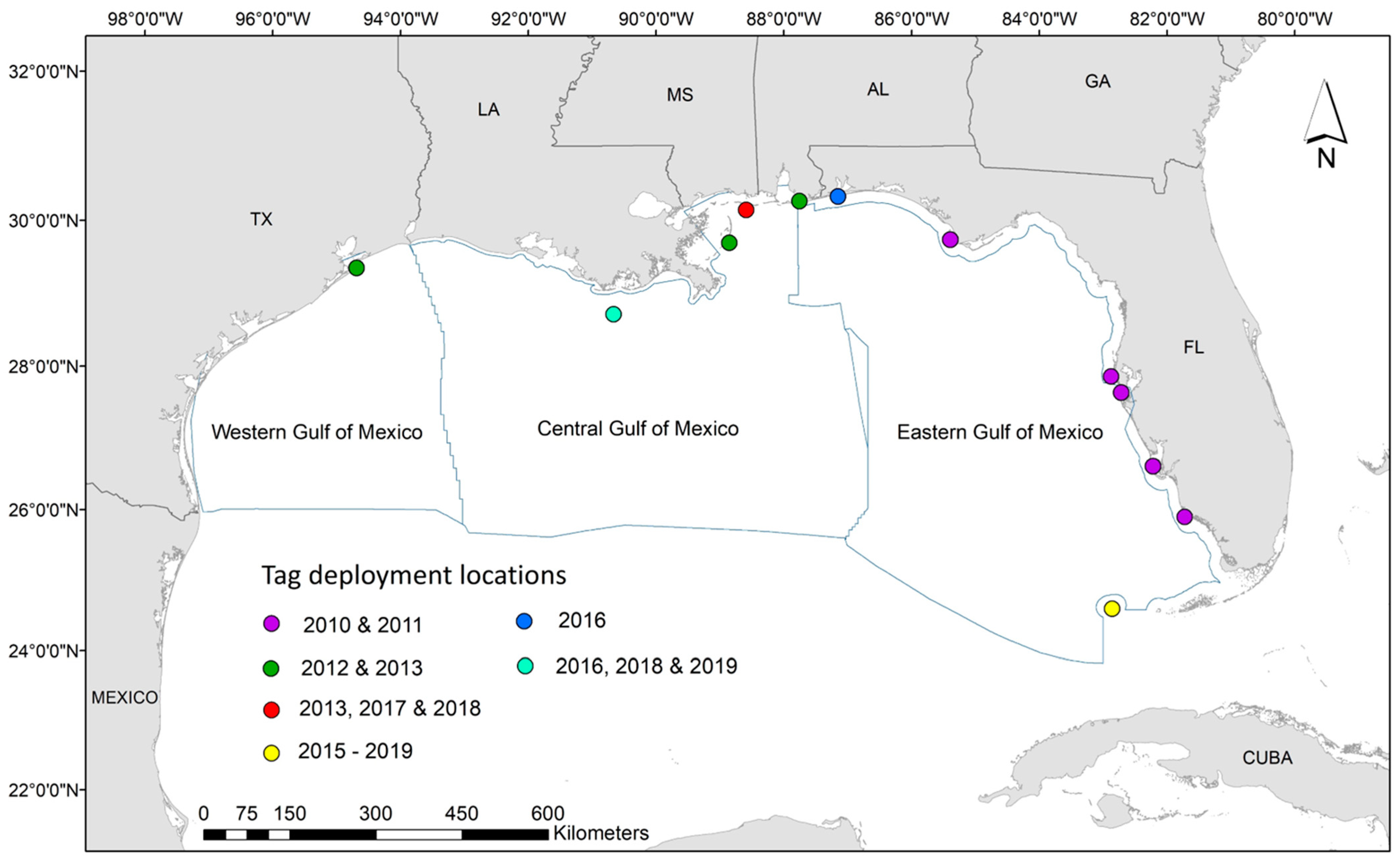
2.1. Data Collection

All turtles were captured and tagged in various locations throughout the Gulf of Mexico (i.e., Texas, Louisiana, Mississippi, Alabama, or Florida; Figure 1), following methods identical to those in previous studies (e.g., [38]). Per funding and permit requirements, only sub-adult or adult turtles (i.e., carapace length >40 cm) were tagged to ensure animals were large enough to be seen by aerial observers. Briefly, following standard morphometric data collection, we attached platform transmitter terminals (PTT) to the turtle carapace using slow-curing epoxy (two-part Superbond epoxy). Data were collected via specialized depth-logging satellite tags (Wildlife Computers SPLASH10-309A and SPLASH10-238A-AF; tag specifications available in Supplementary Materials) from 2010–2019. Each of the 136 tags was programmed to collect dive activity information 24 h a day by ‘binning’ the data into a pre-specified number of bins throughout the summary period. Data were then transmitted once a day through the Argos satellite system. Beginning in 2011, all satellite tags on nesting loggerheads were optimized in an effort to preserve battery life by setting transmission to every third day from 1 November through 1 April [38]. We utilized the time-at-depth (TAD; percent time within depth bins) component of the tag summary and set depth bins at 0, 1, 2, 3, 4, 5, 10, 20, 30, 40, 50, 100, 150, and >150 m. Depth bins from 0–2 m were collectively defined as the surface of the water and correspond to depths where turtles are assumed visible to observers during aerial surveys. As our focus for this analysis was time at surface (TAS), we organized the data as the proportion of time per day that the turtle spent at the surface and disregarded all other depth bins. We used a daily scale for all turtles regardless of species or spatial location due to irregularities in the data collection and satellite transmission periods throughout the study duration. Dive data were then formatted so each daily point contained information on the proportion of time spent at surface, the date, and all relevant metadata (i.e., species, sex, capture method (i.e., nester or in-water), and tagging location).

2.2. Linking Spatial and Dive Data

We linked spatial location to each dive observation by performing a switching state space model (SSM) on the raw location data. The SSM approach was used to estimate the animals’ true locations at regular time intervals due to significant positional uncertainty in the Argos data [6] and to generate daily locations on which to annotate the proportion of TAS. All turtles were pooled for the SSM in order to more precisely estimate daily spatial locations and movement parameters [39,40]. Briefly, following previous analyses [6,41], we used a Bayesian hierarchical movement model implemented in the R package ‘bsam’ [40,42], using the ‘hDCRWS’ model specification and a time step of 1 day to match the TAS data. We set the Markov Chain Monte Carlo (MCMC) parameters following Roberts et al. [6], which used adaptive sampling for 7000 draws, taking 10,000 samples from the posterior distribution, and then thinning by five to reduce MCMC autocorrelation, resulting in 2000 posterior samples from which to make inference. Trace plots, diagnostic plots, and ACF plots were utilized to visually assess sufficient model convergence [40,43]. The SSM process ultimately resulted in a more accurate dataset by accounting for location errors and provided 1 location point for each turtle per day. We then linked SSM output to the TAS data using the unique turtle ID and date.

2.3. Environmental and Oceanographic Variables

We identified 11 remotely sensed environmental or oceanographic parameters that have known or plausible roles in influencing turtle dive behavior (Table 1) [12,13]. For the static variables (i.e., distance to shore/shelf and bathymetry), we obtained gridded layers and extracted the raster value using the ‘raster’ package in R at each turtle location in the dive data. Daily sea surface temperature (SST) and SST anomaly (SSTa) gridded layers were downloaded at a 0.04 decimal degree resolution from the NOAA ERDDAP online repository for the duration of our tracking period (2010–2019; https://coastwatch.pfeg.noaa.gov/erddap/griddap/ncdcOisst2Agg.html (accessed on 1 March 2020)). Each daily SST and SSTa value were paired spatially with the dive information using the ‘raster’ package. We downloaded daily netCDF files (also at a 0.04 decimal degree resolution) for surface salinity, sea surface height (SSH), and u and v vector surface currents from the Gulf of Mexico HYCOM project (https://www.hycom.org/data/goml0pt04/ (accessed on 1 March 2020)) [22]. The ‘ncdf4’ R package was used to extract the variables with the associated longitude, latitude, and date and organize all into a single data frame. In order to pair each variable with the daily observations in the dive data, we found the minimum spatial difference between each point in the dive data and each HYCOM variable. Current strength (i.e., absolute current) and current direction were calculated using the u and v vector components.
To explore the potential relationship between the ocean frontal features and turtle time at surface, we analyzed the dataset describing ocean color and thermal frontal zones in the Gulf of Mexico [24]. The dataset was generated by applying a gradient-based front detection algorithm [44] to the daily MODIS/Aqua SST and color index (CI) [45] measurements between 2002 and 2019. Its spatial and temporal resolutions are 9 km and weekly, respectively. In the weekly maps, each location is described by its mean frontal gradient magnitude (FGM); more details on this dataset can be found in Zhang and Hu [24]. The FGM value corresponding to each turtle data record (latitude, longitude, date) was extracted and analyzed with other turtle-relevant data. Individual observations for all predictor variables were identified as outliers and removed from subsequent analyses if they fell more than two standard deviations away from their mean (less than 3% of the entire dataset). We ensured the removal of outliers had no effect on model performance by comparing GAM summary metrics (details in Section 2.4) prior to and after removal. All organization and formatting of environmental data was performed in Program R (Version 4.0.3) [46].

2.4. Quantifying Environmental Influence on Time at Surface

To determine which environmental or oceanographic parameters influence the proportion of time turtles spend at the surface, we used a generalized additive modeling (GAM) approach with a beta error distribution appropriate for proportional data scaled between 0 and 1 and logit link; we fit GAMs using the R package ‘mgcv’ [47]. The data were first separated by species, as we aim to contribute to species-specific density estimates and aerial correction factors. For each species model, we randomly partitioned the data with approximately 70% being used for model training and 30% used for model testing or evaluation. This 70/30 split occurred at the scale of the individual turtle, rather than the daily observation, to ensure model training and testing encompassed the entirety of a turtle’s track. Additionally, this process retained the model structure within the dataset used for model evaluation and ensured that predicted values were generated on complete turtle tracks that were not included in model development. Following a data exploration of each variable, we determined that a logarithmic transformation was necessary for salinity and depth. All continuous variables were then assessed for collinearity using the Pearson correlation coefficient method to ensure accurate predictions. A collinearity threshold value of 0.7 was applied to reject the use two or more variables in the same model [48].
We set a maximum of 5 knots for each covariate to avoid overfitting and specified the restricted maximum likelihood (REML) method. Planning region of the Gulf of Mexico as defined by the U.S. Department of the Interior Bureau of Ocean Energy Management (BOEM; Figure 1) and season were incorporated as factor variables and unique turtle ID was included as a random effect. Following an examination of the spatial pattern in residuals, we also included spatial smooths for easting and northing in each species model. Covariates (including factor variables) were only kept in each model if its inclusion resulted in a lower Akaike’s Information Criterion (AIC) value for the overall model. A ΔAIC threshold of >2 was used to determine if an added covariate improved the model. For each GAM, we checked the basis dimension values for each smooth term to ensure the correct number of knots were present [47]. Pairwise concurvity was also analyzed to ensure close relationships did not exist between the smooth terms. Model performance was assessed using the adjusted R2 value and the amount of deviance explained. Additionally, we quantified the model error or confidence in the resulting probability estimates for both the testing and training datasets. Model error was displayed using the coefficient of variation (CV), which is the ratio of the root mean squared error (RMSE) to the predicted value per observation. Spatial predictions and associated model uncertainty were then aggregated into a regularized 10 × 10 km2 grid for visual purposes.

3. Results

3.1. Data Collection

Throughout the 10-year tagging effort, we deployed 136 depth tags onto three species of marine turtles: loggerhead (Caretta caretta; n = 59), Kemp’s ridley (Lepidochelys kempii, n = 63), and green (Chelonia mydas, n = 14). Of these 136, 47 were tagged in Florida; 45 were tagged in Alabama; 26 were tagged in Mississippi; 13 were tagged in Louisiana; and 5 were tagged in Texas (Figure 1) [49]. Mean tracking duration across the three species was 130 days, with 100 days on average for Kemp’s ridley (LK), 156 days for loggerheads (CC), and 163 days for green turtles (CM; Supplementary Materials: Figures S1 and S2). We used a total of 100,475 Argos locations to run the SSM, after filtering for extreme outliers and removing those observations without a location class. Four individuals (tag IDs 161454, 172675, 175680, and 100391) were hindering the fit of the SSM due to inadequate tracking duration (i.e., <10 days) [6] and were removed from further analysis. After fitting the SSM, we were left with a total of 11,451 daily locations for 132 turtles (Supplementary Materials: Figure S3).

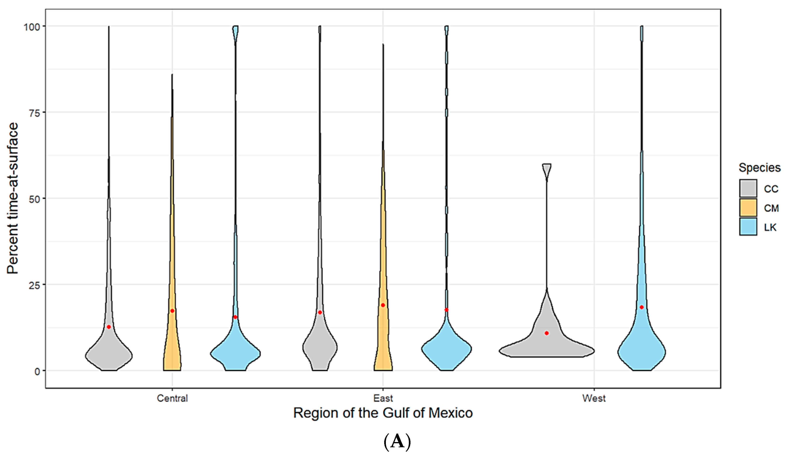
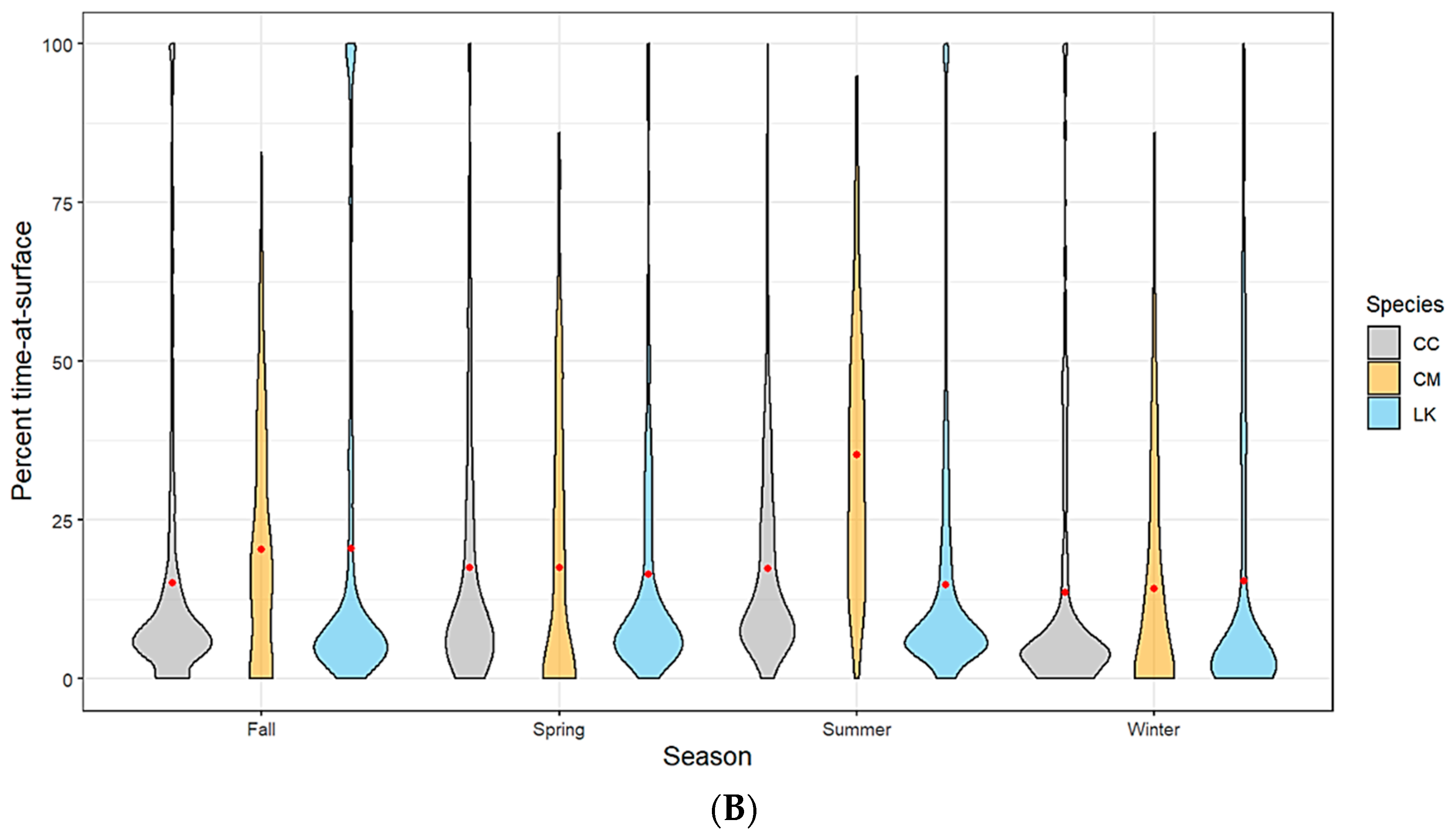
3.2. Time-at-Surface Summaries

Kemp’s ridley turtles, the most well represented species in our analysis, spent on average 18% of the time at the surface (TAS) across all spatial locations with no seasonal variability. Loggerheads spent on average approximately 16% of the time at the surface. This average was slightly lower for the western planning area of the Gulf, likely due to a lack of tracking data for this species as most tagged individuals hugged the Florida coastline and only moved as far west as Louisiana (Figure 2A). Loggerhead TAS also dropped slightly during the winter months and peaked during summer, which coincides with the timing of nesting season (Figure 2B). While we have a much lower sample size from which to draw conclusions for green turtles, our data suggests that this species has a slightly higher mean TAS than the other two species (19%). Additionally, the range of TAS for green turtles is wider when examined across all individuals. We did not track any green turtles into the western planning region (Figure 2A). Time spent at the surface for green turtles peaked in summer, which coincides with nesting season activity (Figure 2B).

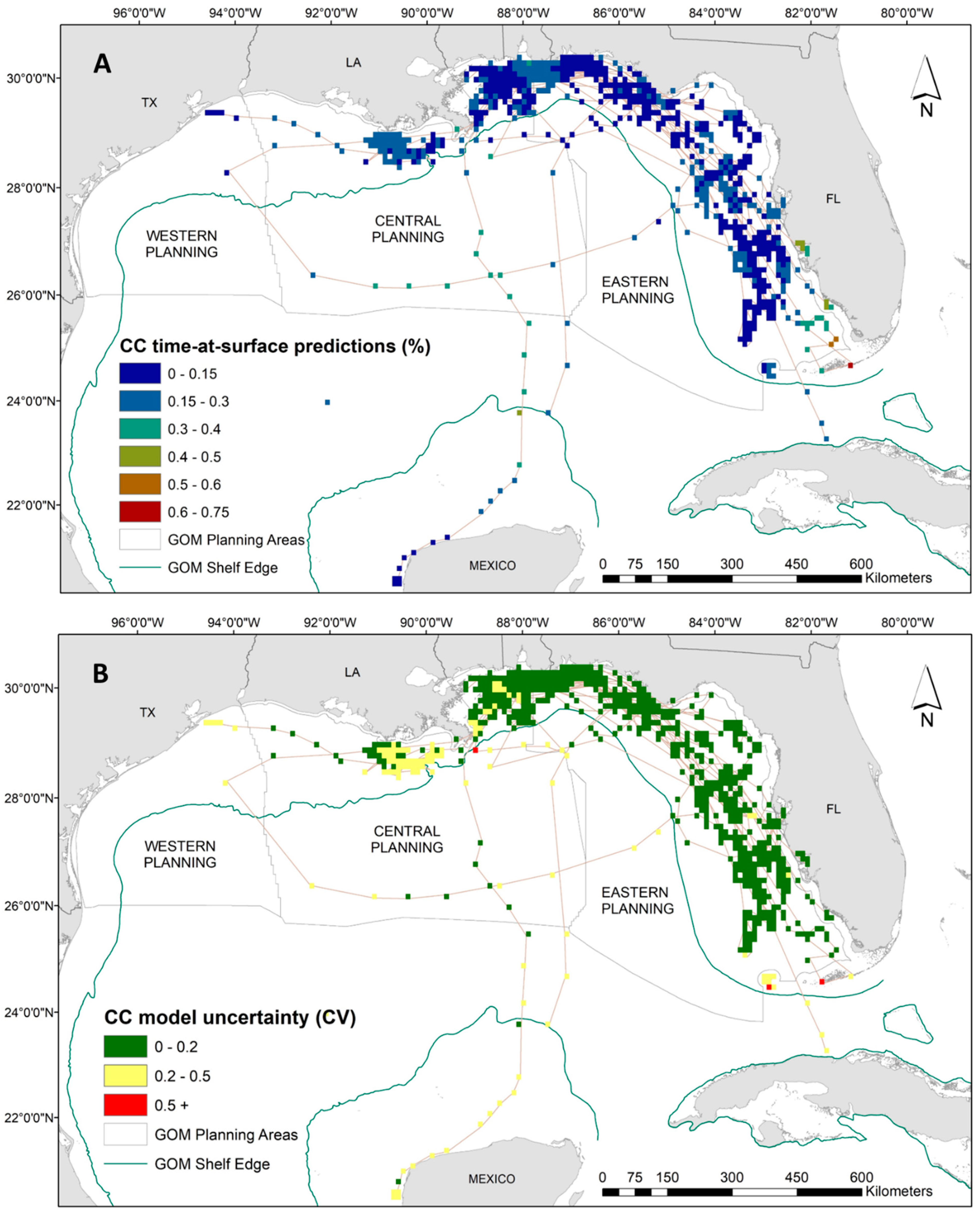
3.3. Modeling Time at Surface

Results from the GAM demonstrated that loggerheads spent a higher proportion of time at the surface in warmer waters (i.e., between 25 °C and 30 °C), shallow to intermediate depth ranges, and all but the highest measured salinities (Supplementary Materials: Figure S4). The increased presence of a front, both SST and ocean color derived, also increased surface time in loggerheads. However, particularly strong SST fronts decreased time at surface. Additionally, increased surface time coincided with spring and summer months, which is consistent with loggerhead nesting season. Spatial predictions show that loggerhead TAS proportions are highest off the coast of southwest Florida and in parts of the Florida Keys, with a maximum TAS value of 74% (Figure 3A). For the remainder of the loggerhead tracking footprint in the Gulf, our results show there is minimal variability in TAS. (Figure 3A). Spatial output of model uncertainty for the loggerhead time-at-surface model (represented by the coefficient of variation) reveals high confidence (i.e., below 0.5) in the majority of predictions with the exception of several observations along the Florida Keys reef tract and one off the Louisiana coast (Figure 3B).
Our results indicate that Kemp’s ridley turtles occupy a wide temperature range at the surface (i.e., between 20 °C and 35 °C) with close proximity to the continental shelf, and very shallow waters (i.e., below 30 m). Neither frontal product was significant to the Kemp’s ridley model, and no relationship was evident to time at surface (Supplementary Materials: Figure S5). Spatial predictions demonstrate the substantial latitudinal gradient for the Kemp’s ridley model compared to the loggerheads and greens, which results in more variability in proportions of time at the surface (Figure 4A). Higher surface intervals (i.e., above 45%) were predicted between the continental shelf and Louisiana coastline, while the majority throughout the rest of the Gulf ranged between 10% and 40% (Figure 4A). Despite the widespread tracking footprint, we achieved majority low model uncertainty (i.e., CV less than 0.2) in the predictions generated for the Kemp’s ridley model (Figure 4B). Potentially due to limited data in the area, we have higher uncertainty in interpreting the predictions off the coast of Mexico and into the Yucatan Peninsula as well as along the western coast of Florida (Figure 4B).
While we have a lower sample size for green turtles, the distribution of tracking data is notably unique from the other two species in the proximity to the coastline. Therefore, our interpretation of dive behavior for green turtles can serve as an important first step in delineating species-specific environmental associations. Results from the GAM for the 14 green turtles suggested that higher time-at-surface proportions were closely related to spring months, shallow waters, warmer than average SST (based on anomaly calculation; Table 1), and stronger/more persistent SST fronts (Supplementary Materials: Figure S6). The increased presence of ocean color fronts decreased the time spent at the surface in green turtles. The tendency for green turtles to stay in close proximity to the coastline is demonstrated in Figure 5A. These spatial predictions also reveal significant variability in surface intervals, similar to the Kemp’s ridleys, even among 14 individuals. We see the highest predicted time at surface for the green turtles along the Florida panhandle and off the coast of Louisiana (Figure 5A). Associated uncertainty in these predictions is high due to low sample size (Figure 5B). For this species, we therefore concentrate our conclusions along sections of the Florida coastline where uncertainty is lower (Figure 5B).

4. Discussion

Conservation measures that target migratory species frequently rely on a comprehensive assessment of habitat preferences and space use, often obtained from satellite tracking data and species distribution models. Their use of three-dimensional space, however, and how their environment influences this behavior is still emerging as an integral component to understanding species’ ecology and life history [9,12]. Here, we present the environmental and oceanographic influence on time-at-surface patterns for 132 marine turtles across three species, the largest dataset on dive behavior for the Gulf of Mexico region. We incorporated 11 satellite-derived environmental variables into the models, several of which have never been examined in the context of marine turtle distribution or dive patterns. In addition to defining seasonal and spatial differences in time-at-surface patterns, we found species-specific associations of environmental covariates related to increased time at surface, particularly for frontal features, depth, and salinity.
The complexity of dive and surface behavior in marine turtles can result in discrepancies among species, study area, or time of year [12,33]. For example, Hatch et al. [33] examined dive-surfacing behavior, including proportion of time at the surface, for loggerhead turtles in the Northwest Atlantic and reported an average TAS of approximately 50%, compared to an average TAS of 16% found in this study for the same species. Another study that focused on green turtles in the Torres Strait found that approximately 23% of recorded dive time was spent between 0 and 2.5 m of depth [50], which is comparable to our finding of 19% TAS on average for green turtles in the Gulf of Mexico. These patterns or differences could be the product of a myriad of explanatory variables related to foraging, physiological factors, or environmental conditions. Furthermore, there are other potential drivers of increased TAS that our models cannot account for, such as warmer temperatures resulting in higher metabolic rates and therefore requiring higher oxygen consumption.
Many studies have demonstrated a connection between oceanographic features, such as fronts, eddies and currents, and the life cycles of marine migratory species [24,36,51]. Species often use changes in these environmental features as cues for feeding, migration, etc.; therefore, these features are crucial to systematically evaluate when interpreting biologging data [52,53]. One interesting result of our model is the species-specific relationship to frontal features, incorporated into the models as ocean color and SST frontal gradient magnitude (FGM). Both frontal products were significant to loggerhead and green turtles, but neither were included in the Kemp’s ridley final model. One possible explanation for this result is that Kemp’s prefer much shallower water while they are at the surface compared to the other two species, based on the 63 individuals included in this analysis. While frontal behavior in shallow, coastal areas is often difficult to quantify, these fronts can be narrower and less stable than their deep-ocean counterparts [24]. Our results from the loggerhead dive model are similar with previous research [36] in determining that increased TAS for this species is associated with increased frontal activity, suggesting these turtles are possibly exploiting these highly productive areas for foraging purposes similar to other marine megafauna [54,55]. Also consistent with previous research, although our sample size is limited, surface time in green turtles was associated with frontal features [56]. Similar to loggerheads, green turtles may be engaging with fronts at the surface due to increased productivity in these areas.
The improvement in remotely-sensed environmental data has allowed for the emergence of novel predictor variables to be utilized in modeling frameworks. In addition to including ocean frontal features in our GAMs as well as variables such as SST and bathymetry that have demonstrated relationships to marine turtle dive behavior [12,32], we also explored the relationship between time at surface and current strength and direction, calculated from U and V component vectors [22]. While neither variable was significant to any species model, potentially due to the daily scale at which this analysis was performed, the influence of oceanic currents on species’ trajectories has previously been detected [52,57]. Where oceanic currents are incorporated into movement models, results have shown that some marine predators exhibit highly directional movement even in the face of strong currents for foraging or migrating purposes [52,58] and will often select areas of high-current to reduce their energy expenditure [59]. Remotely sensed products will only improve in complexity, comprehensiveness, and resolution moving forward [60]. While the numerous predictor variables included in this analysis represent the most wide-ranging assessment to understand marine turtle surface behavior to date, further environmental drivers can be explored as they become available to improve predictions.
Marine turtles face a multitude of threats in the ocean, such as entanglement in fishing gear, pollution, habitat destruction and vessel strikes [61]. Risk assessments have often concluded that these threats are exacerbated in shallow, coastal habitats due to their relative importance for foraging and development; thus, heavily contributing to the anthropogenic mortality of turtle species [62]. Collisions with vessels, for example, have increased in recent decades as a result of high-density recreational boat traffic in coastal areas and often minimal regulation or enforcement on vessel speed [61]. For three imperiled turtle species, this analysis provides descriptive statistics on how often (on average) turtles can be found at the surface within the Gulf of Mexico as well as environmental conditions associated with an increase in surface activity and could therefore be implemented into conservation strategies to assess risk and minimize vessel-related mortality. Existing or proposed spatial management efforts, such as no-wake zones or human exclusion zones, could be informed by our results and potentially implemented under a dynamic framework to allow for rapid adjustments in space and time [29]. Additionally, knowledge of marine turtle surface behavior could be valuable for fisheries management in the Gulf of Mexico, as certain gear types are known to unintentionally but frequently capture turtles [62].
We have identified the main sources of uncertainties in our analysis. First, the collection of the dive activity data spanning multiple projects across ten years resulted in inconsistencies in tag programming, thus eliminating our ability to delineate day versus night dive behavior. This assumption, that marine turtle time at surface remains the same throughout the day, potentially distorts our results as all possible satellite transmissions throughout a 24 h time period were aggregated. This analysis therefore can serve as a baseline for elucidating time-at-surface behavior in the Gulf of Mexico at the species level and can be updated prior to inclusion in any management or action framework. Additionally, due to this 24 h applied scale and the inherent flaws in inferring animal behavior from position and dive data, we were unable to accurately define foraging at the surface. Future work could utilize recent advances in animal movement modeling (e.g., [63,64]), to differentiate foraging strategies among individuals and potentially evaluate foraging success at the population level. Finally, addressing how marine turtle surface patterns are linked to changing climatic and oceanographic conditions, although a key priority area for dynamic management [65], was beyond the scope of this analysis. However, a larger spatial coverage due to increased tag deployments, increased diversity in climatic variables, and a longer study duration could determine if observed environmental influences on time at surface are shifting over time and whether these shifts could be attributed to climate change.
Understanding the spatiotemporal distribution of protected species is a key component in developing conservation strategies and mitigating potential human impacts. Species distribution models that evaluate species–environment relationships and use these to characterize animal density or occurrence across broad spatial and temporal scales are routinely used to support environmental impact assessments [66,67]. The data underlying these models are primarily visual line-transect survey data (e.g., [68]). In the case of sea turtles in the Gulf of Mexico, these data are collected through aerial surveys over the continental shelf (e.g., [69]). However, sea turtles spend a significant portion of their time below the water surface, and this is a source of substantial negative bias in density estimates derived from visual surveys. Furthermore, spatiotemporal variation in the probability that turtles are at the surface may further bias the inferred spatial patterns in animal distribution. Our models can be used to directly estimate availability at the surface for visual surveys based upon contemporaneous oceanographic conditions and animal location and thereby address this known bias and improve the reliability of resulting spatial density models.

5. Conclusions

In this study, we have demonstrated how marine turtle surface patterns can be linked to environmental and oceanographic variables and how this behavior varies seasonally and by species. To our knowledge, this unique dataset on turtle dive behavior is the largest available for the Gulf of Mexico, encompassing over 10 years of depth-logging and satellite tracking information. Furthermore, we illustrate how this analysis can be integrated into future work on density and abundance modeling for the Gulf of Mexico’s broader ecosystem to improve our understanding of how marine turtles utilize this important region. For further population monitoring, results from the GAMs reveal that loggerhead turtles are more available to be seen by aerial surveys off the southwest Florida coastline, Kemp’s ridleys off Louisiana and Texas, and green turtles along the western Florida coastline. These results support a strategy whereby each species would be managed independently, which could lead to a more accurate estimation of species-specific foraging habitats and impacts on trophic resources. Increasingly reliable, spatially-explicit models on distribution and behavior of imperiled species can inform decisions related to the Endangered Species Act and other regulatory needs. This analysis contributes to ongoing discussions of critical habitat designations for marine turtles in the Gulf of Mexico and highlights the importance of quantifying their use of the water column for the purpose of risk mitigation and adaptive management.

Supplementary Materials

The following supporting information can be downloaded at: https://www.mdpi.com/article/10.3390/rs14184534/s1, Figure S1: Tracking duration of all marine turtles included in the analysis from mid-2010 until January of 2016. Colors represent region of the Gulf of Mexico as defined by Bureau of Ocean Energy Management (BOEM); Figure S2: Tracking duration of all marine turtles included in the analysis from January 2016 until mid-2019. Colors represent region of the Gulf of Mexico as defined by Bureau of Ocean Energy Management (BOEM); Figure S3: Resulting tracks from state space model for all marine turtles included in the analysis separated by species; Figure S4: Generalized additive model (GAM) plots of loggerhead turtle (Caretta caretta) time-at-surface (scaled between 0 and 1) in the Gulf of Mexico relative to environmental and factor variables. Shaded areas for environmental variable plots represent standard error; Figure S5: Generalized additive model (GAM) plots of Kemp’s ridley turtle (Lepidochelys kempii) time-at-surface (scaled between 0 and 1) in the Gulf of Mexico relative to environmental and factor variables. Shaded areas for environmental variable plots represent standard error; Figure S6: Generalized additive model (GAM) plots of green turtle (Chelonia mydas) time-at-surface (scaled between 0 and 1) in the Gulf of Mexico relative to environmental and factor variables. Shaded areas for environmental variable plots represent standard error.

Author Contributions

Conceptualization, K.E.R. and K.M.H.; methodology, K.E.R., L.P.G., J.O.-O., C.H. and K.M.H.; formal analysis, K.E.R., L.P.G., Y.Z., J.O.-O. and C.H.; resources, C.R.S., J.O.-O. and M.L.; data curation, K.E.R., C.H. and Y.Z.; writing—original draft preparation, K.E.R.; writing—review and editing, K.E.R., L.P.G., K.M.H., C.R.S. and M.L.; project administration, K.M.H. and M.L.; funding acquisition, K.M.H. and M.L. All authors have read and agreed to the published version of the manuscript.

Funding

We acknowledge funding for various aspects of the tagging portion of this project from the U.S. Geological Survey (USGS) Ecosystems Mission Area Species Management Research program, the USGS Priority Ecosystems Science Program, the USGS Coastal and Marine Geology Program, the USGS Natural Resource Protection Program, Natural Resource Damage Assessment for the Deepwater Horizon Oil Spill and the National Park Service. Numerous permits from several authorities across multiple states and territories have made our research possible. Permits issued to K. Hart include: MTP176; NMFS permits 20315, 17381, 13307, 16146, 22281; NPS permits EVER-2018-SCI-0023, EVER-2016-SCI-0032, EVER-2014-SCI-0031, DRTO-2018-SCI-0007, DRTO-2016-SCI-0008, DRTO-2014-SCI-0004, DRTO-2012-SCI-0008, DRTO-2010-SCI-0009, DRTO-2008-SCI-0008, Federal U.S. Fish and Wildlife Permit #TE98424B-1 and #TE98424B-0 (Baldwin County, Alabama); and Bon Secour National Wildlife Refuge Special Use Permit #16-005S, 12-006S. Work was also performed under a USFWS permit issued to J. Philips: TE206903-1. Sampling was approved under Institutional Animal Care and Use protocols USGS-SESC 2011-05, USGS SESC 2014-03, SER-BISC-BUIS-DRTO-EVER-Hart-Sea Turtles-Terrapins-2018-A2.

Data Availability Statement

All data are available at Hart et al. [49].

Acknowledgments

We thank the following U.S. Geological Survey staff and contractors who were critical to the field portion of this study: Mike Cherkiss, David Roche, Andrew Crowder, Mat Denton, Megan Arias, Devon Nemire-Pepe, Brian Smith, Derek Burkholder, and Thomas Selby. Numerous USGS volunteers also assisted with field work over the years. We thank National Park Service interns and colleagues Tracy Ziegler Tree Gottshall, Glenn Simpson, Meaghan Johnson, Kayla Nimmo, Allen Zamrock, Janie Douglass, Clay ‘Blue’ Douglass, John Spade, Mikey Kent, Tylan Dean, and Dave Hallac. Any use of trade, firm, or product names is for descriptive purposes only and does not imply endorsement by the U.S. Government.

Conflicts of Interest

The authors declare no conflict of interest.

References

  1. Pinsky, M.L.; Selden, R.L.; Kitchel, Z.J. Climate-Driven Shifts in Marine Species Ranges: Scaling from Organisms to Communities. Annu. Rev. Mar. Sci. 2020, 12, 153–179. [Google Scholar] [CrossRef] [PubMed]
  2. Gill, J.A.; Alves, J.A.; Gunnarsson, T.G. Mechanisms Driving Phenological and Range Change in Migratory Species. Philos. Trans. R. Soc. B Biol. Sci. 2019, 374, 20180047. [Google Scholar] [CrossRef] [PubMed]
  3. Simmonds, M.P.; Isaac, S.J. The Impacts of Climate Change on Marine Mammals: Early Signs of Significant Problems. Oryx 2007, 41, 19–26. [Google Scholar] [CrossRef]
  4. Wisz, M.S.; Pottier, J.; Kissling, W.D.; Pellissier, L.; Lenoir, J.; Damgaard, C.F.; Dormann, C.F.; Forchhammer, M.C.; Grytnes, J.A.; Guisan, A.; et al. The Role of Biotic Interactions in Shaping Distributions and Realised Assemblages of Species: Implications for Species Distribution Modelling. Biol. Rev. 2013, 88, 15–30. [Google Scholar] [CrossRef] [PubMed]
  5. Selig, E.R.; Turner, W.R.; Troëng, S.; Wallace, B.P.; Halpern, B.S.; Kaschner, K.; Lascelles, B.G.; Carpenter, K.E.; Mittermeier, R.A. Global Priorities for Marine Biodiversity Conservation. PLoS ONE 2014, 9, e82898. [Google Scholar] [CrossRef] [PubMed]
  6. Roberts, K.E.; Smith, B.J.; Burkholder, D.; Hart, K.M. Evaluating the Use of Marine Protected Areas by Endangered Species: A Habitat Selection Approach. Ecol. Solut. Evid. 2021, 2, e12035. [Google Scholar] [CrossRef]
  7. Pérez-Jorge, S.; Tobeña, M.; Prieto, R.; Vandeperre, F.; Calmettes, B.; Lehodey, P.; Silva, M.A. Environmental Drivers of Large-Scale Movements of Baleen Whales in the Mid-North Atlantic Ocean. Divers. Distrib. 2020, 26, 683–698. [Google Scholar] [CrossRef]
  8. Serratosa, J.; Hyrenbach, K.D.; Miranda-Urbina, D.; Portflitt-Toro, M.; Luna, N.; Luna-Jorquera, G. Environmental Drivers of Seabird At-Sea Distribution in the Eastern South Pacific Ocean: Assemblage Composition Across a Longitudinal Productivity Gradient. Front. Mar. Sci. 2020, 6, 838. [Google Scholar] [CrossRef]
  9. Hochscheid, S. Why We Mind Sea Turtles’ Underwater Business: A Review on the Study of Diving Behavior. J. Exp. Mar. Biol. Ecol. 2014, 450, 118–136. [Google Scholar] [CrossRef]
  10. Roncon, G.; Bestley, S.; McMahon, C.R.; Wienecke, B.; Hindell, M.A. View from below: Inferring Behavior and Physiology of Southern Ocean Marine Predators from Dive Telemetry. Front. Mar. Sci. 2018, 5, 464. [Google Scholar] [CrossRef] [Green Version]
  11. Bauer, R.K.; Fromentin, J.-M.; Demarcq, H.; Bonhommeau, S. Habitat Use, Vertical and Horizontal Behaviour of Atlantic Bluefin Tuna (Thunnus thynnus) in the Northwestern Mediterranean Sea in Relation to Oceanographic Conditions. Deep Sea Res. Part II Top. Stud. Oceanogr. 2017, 141, 248–261. [Google Scholar] [CrossRef]
  12. Iverson, A.R.; Fujisaki, I.; Lamont, M.M.; Hart, K.M. Loggerhead Sea Turtle (Caretta caretta) Diving Changes with Productivity, Behavioral Mode, and Sea Surface Temperature. PLoS ONE 2019, 14, e0220372. [Google Scholar] [CrossRef] [PubMed]
  13. Fukuoka, T.; Suganuma, H.; Kondo, S.; Sato, K. Long Dive Capacity of Olive Ridley Turtles (Lepidochelys olivacea) at High Water Temperature during the Post-Nesting Foraging Period in the Arafura Sea. J. Exp. Mar. Biol. Ecol. 2022, 546, 151649. [Google Scholar] [CrossRef]
  14. Freitas, C.; Caldeira, R.; Reis, J.; Dellinger, T. Foraging Behavior of Juvenile Loggerhead Sea Turtles in the Open Ocean: From Lévy Exploration to Area-Restricted Search. Mar. Ecol. Prog. Ser. 2018, 595, 203–215. [Google Scholar] [CrossRef]
  15. Owen, K.; Jenner, K.C.S.; Jenner, M.N.M.; McCauley, R.D.; Andrews, R.D. Water Temperature Correlates with Baleen Whale Foraging Behaviour at Multiple Scales in the Antarctic. Mar. Freshw. Res. 2019, 70, 19–32. [Google Scholar] [CrossRef]
  16. Madrak, S.; Lewison, R.; Eguchi, T.; Klimley, A.; Seminoff, J. Effects of Ambient Temperature on Dive Behavior of East Pacific Green Turtles before and after a Power Plant Closure. Mar. Ecol. Prog. Ser. 2022, 683, 157–168. [Google Scholar] [CrossRef]
  17. McIntyre, T.; Ansorge, I.J.; Bornemann, H.; Plötz, J.; Tosh, C.A.; Bester, M.N. Elephant Seal Dive Behaviour Is Influenced by Ocean Temperature: Implications for Climate Change Impacts on an Ocean Predator. Mar. Ecol. Prog. Ser. 2011, 441, 257–272. [Google Scholar] [CrossRef]
  18. Arrowsmith, L.; Sequeira, A.; Pattiaratchi, C.; Meekan, M. Water Temperature Is a Key Driver of Horizontal and Vertical Movements of an Ocean Giant, the Whale Shark Rhincodon typus. Mar. Ecol. Prog. Ser. 2021, 679, 101–114. [Google Scholar] [CrossRef]
  19. Loredo, S.A.; Orben, R.A.; Suryan, R.M.; Lyons, D.E.; Adams, J.; Stephensen, S.W. Spatial and Temporal Diving Behavior of Non-Breeding Common Murres during Two Summers of Contrasting Ocean Conditions. J. Exp. Mar. Biol. Ecol. 2019, 517, 13–24. [Google Scholar] [CrossRef]
  20. Brodie, S.J.; Thorson, J.T.; Carroll, G.; Hazen, E.L.; Bograd, S.; Haltuch, M.A.; Holsman, K.K.; Kotwicki, S.; Samhouri, J.F.; Willis-Norton, E.; et al. Trade-Offs in Covariate Selection for Species Distribution Models: A Methodological Comparison. Ecography 2020, 43, 11–24. [Google Scholar] [CrossRef] [Green Version]
  21. Arenas-Castro, S.; Regos, A.; Gonçalves, J.F.; Alcaraz-Segura, D.; Honrado, J. Remotely Sensed Variables of Ecosystem Functioning Support Robust Predictions of Abundance Patterns for Rare Species. Remote Sens. 2019, 11, 2086. [Google Scholar] [CrossRef]
  22. Chassignet, E.P.; Hurlburt, H.E.; Smedstad, O.M.; Halliwell, G.R.; Hogan, P.J.; Wallcraft, A.J.; Baraille, R.; Bleck, R. The HYCOM (HYbrid Coordinate Ocean Model) Data Assimilative System. J. Mar. Syst. 2007, 65, 60–83. [Google Scholar] [CrossRef]
  23. Shepard, A.N.; Valentine, J.F.; D’Elia, C.F.; Yoskowitz, D.W.; Dismukes, D.E. Economic Impact of Gulf of Mexico Ecosystem Goods and Services and Integration into Restoration Decision-Making. Gulf Mex. Sci. 2013, 31, 10–27. [Google Scholar] [CrossRef]
  24. Zhang, Y.; Hu, C. Ocean Temperature and Color Frontal Zones in the Gulf of Mexico: Where, When, and Why. J. Geophys. Res. Ocean. 2021, 126, e2021JC017544. [Google Scholar] [CrossRef]
  25. Valverde, R.A.; Holzwart, K.R. Sea Turtles of the Gulf of Mexico BT—Habitats and Biota of the Gulf of Mexico: Before the Deepwater Horizon Oil Spill. In Volume 2: Fish Resources, Fisheries, Sea Turtles, Avian Resources, Marine Mammals, Diseases and Mortalities; Ward, C.H., Ed.; Springer: New York, NY, USA, 2017; pp. 1189–1351. ISBN 978-1-4939-3456-0. [Google Scholar]
  26. Rabotyagov, S.S.; Kling, C.L.; Gassman, P.W.; Rabalais, N.N.; Turner, R.E. The Economics of Dead Zones: Causes, Impacts, Policy Challenges, and a Model of the Gulf of Mexico Hypoxic Zone. Rev. Environ. Econ. Policy 2014, 8, 58–79. [Google Scholar] [CrossRef]
  27. Wilson, M.; Tucker, A.D.; Beedholm, K.; Mann, D.A. Changes of Loggerhead Turtle (Caretta caretta) Dive Behavior Associated with Tropical Storm Passage during the Inter-Nesting Period. J. Exp. Biol. 2017, 220, 3432–3441. [Google Scholar] [CrossRef] [PubMed]
  28. Wilson, M.; Bailey, D.; Maung-douglass, E.; Partyka, M.; Sempier, S.; Skelton, T. Advancements in Understanding Ocean Circulation and Tracking the Movements of Oil; GOMSG-G-21-001; National Oceanic and Athmospheric Administration: Silver Spring, MA, USA, 2021. [Google Scholar]
  29. Maxwell, S.M.; Hazen, E.L.; Lewison, R.L.; Dunn, D.C.; Bailey, H.; Bograd, S.J.; Briscoe, D.K.; Fossette, S.; Hobday, A.J.; Bennett, M.; et al. Dynamic Ocean Management: Defining and Conceptualizing Real-Time Management of the Ocean. Mar. Policy 2015, 58, 42–50. [Google Scholar] [CrossRef]
  30. Hart, K.M.; Lamont, M.M.; Iverson, A.R.; Smith, B.J. The Importance of the Northeastern Gulf of Mexico to Foraging Loggerhead Sea Turtles. Front. Mar. Sci. 2020, 7, 330. [Google Scholar] [CrossRef]
  31. Crowe, L.M.; Hatch, J.M.; Patel, S.H.; Smolowitz, R.J.; Haas, H.L. Riders on the Storm: Loggerhead Sea Turtles Detect and Respond to a Major Hurricane in the Northwest Atlantic Ocean. Mov. Ecol. 2020, 8, 32. [Google Scholar] [CrossRef]
  32. Wildermann, N.E.; Sasso, C.R.; Stokes, L.W.; Snodgrass, D.; Fuentes, M.M.P.B. Habitat Use and Behavior of Multiple Species of Marine Turtles at a Foraging Area in the Northeastern Gulf of Mexico. Front. Mar. Sci. 2019, 6, 155. [Google Scholar] [CrossRef] [Green Version]
  33. Hatch, J.M.; Haas, H.L.; Sasso, C.R.; Patel, S.H.; Smolowitz, R.J. Estimating the Complex Patterns of Survey Availability for Loggerhead Turtles. J. Wildl. Manag. 2022, 86, e22208. [Google Scholar] [CrossRef]
  34. Polovina, J.J.; Balazs, G.H.; Howell, E.A.; Parker, D.M.; Seki, M.P.; Dutton, P.H. Forage and Migration Habitat of Loggerhead (Caretta caretta) and Olive Ridley (Lepidochelys olivacea) Sea Turtles in the Central North Pacific Ocean. Fish. Oceanogr. 2004, 13, 36–51. [Google Scholar] [CrossRef]
  35. Shillinger, G.L.; Swithenbank, A.M.; Bailey, H.; Bograd, S.J.; Castelton, M.R.; Wallace, B.P.; Spotila, J.R.; Paladino, F.V.; Piedra, R.; Block, B.A. Vertical and Horizontal Habitat Preferences of Post-Nesting Leatherback Turtles in the South Pacific Ocean. Mar. Ecol. Prog. Ser. 2011, 422, 275–289. [Google Scholar] [CrossRef]
  36. Scales, K.L.; Miller, P.I.; Varo-Cruz, N.; Hodgson, D.J.; Hawkes, L.A.; Godley, B.J. Oceanic Loggerhead Turtles Caretta caretta Associate with Thermal Fronts: Evidence from the Canary Current Large Marine Ecosystem. Mar. Ecol. Prog. Ser. 2015, 519, 195–207. [Google Scholar] [CrossRef]
  37. Witherington, B.; Hirama, S.; Hardy, R. Young Sea Turtles of the Pelagic Sargassum-Dominated Drift Community: Habitat Use, Population Density, and Threats. Mar. Ecol. Prog. Ser. 2012, 463, 1–22. [Google Scholar] [CrossRef]
  38. Hart, K.M.; Guzy, J.C.; Smith, B.J. Drivers of Realized Satellite Tracking Duration in Marine Turtles. Mov. Ecol. 2021, 9, 1–14. [Google Scholar] [CrossRef]
  39. Breed, G.A.; Don Bowen, W.; Leonard, M.L. Behavioral Signature of Intraspecific Competition and Density Dependence in Colony-breeding Marine Predators. Ecol. Evol. 2013, 3, 3838–3854. [Google Scholar] [CrossRef]
  40. Jonsen, I. Joint Estimation over Multiple Individuals Improves Behavioural State Inference from Animal Movement Data. Sci. Rep. 2016, 6, 20625. [Google Scholar] [CrossRef]
  41. Hart, K.M.; Lamont, M.M.; Fujisaki, I.; Tucker, A.D.; Carthy, R.R. Common Coastal Foraging Areas for Loggerheads in the Gulf of Mexico: Opportunities for Marine Conservation. Biol. Conserv. 2012, 145, 185–194. [Google Scholar] [CrossRef]
  42. Jonsen, I.D.; Flemming, J.M.; Myers, R.A. Robust State–Space Modeling of Animal Movement Data. Ecology 2005, 86, 2874–2880. [Google Scholar] [CrossRef]
  43. Jonsen, I.D.; Basson, M.; Bestley, S.; Bravington, M.V.; Patterson, T.A.; Pedersen, M.W.; Thomson, R.; Thygesen, U.H.; Wotherspoon, S.J. State-Space Models for Bio-Loggers: A Methodological Road Map. Deep Sea Res. Part II Top. Stud. Oceanogr. 2013, 88, 34–46. [Google Scholar] [CrossRef]
  44. Belkin, I.M.; O’Reilly, J.E. An Algorithm for Oceanic Front Detection in Chlorophyll and SST Satellite Imagery. J. Mar. Syst. 2009, 78, 319–326. [Google Scholar] [CrossRef]
  45. Hu, C. An Empirical Approach to Derive MODIS Ocean Color Patterns under Severe Sun Glint. Geophys. Res. Lett. 2011, 38, L01603. [Google Scholar] [CrossRef]
  46. R Core Team. R: A Language and Environment for Statistical Computing; R Core Team: Vienna, Austria, 2020. [Google Scholar]
  47. Wood, S.N. Generalized Additive Models: An Introduction with R; Chapman and Hall/CRC: Boca Raton, FL, USA, 2017; ISBN 9781315370279. [Google Scholar]
  48. Dormann, C.F.; Elith, J.; Bacher, S.; Buchmann, C.; Carl, G.; Carré, G.; Marquéz, J.R.G.; Gruber, B.; Lafourcade, B.; Leitão, P.J.; et al. Collinearity: A Review of Methods to Deal with It and a Simulation Study Evaluating Their Performance. Ecography 2013, 36, 27–46. [Google Scholar] [CrossRef]
  49. Hart, K.M.; Roberts, K.E.; Lamont, M.; Garrison, L.P.; Sasso, C.R. Surface Time for Sea Turtles in the Gulf of Mexico, 2010–2019; U.S. Geological Survey Data Release, 2022. [Google Scholar] [CrossRef]
  50. Fuentes, M.; Bell, I.; Hagihara, R.; Hamann, M.; Hazel, J.; Huth, A.; Seminoff, J.A.; Sobtzick, S.; Marsh, H. Improving In-Water Estimates of Marine Turtle Abundance by Adjusting Aerial Survey Counts for Perception and Availability Biases. J. Exp. Mar. Biol. Ecol. 2015, 471, 77–83. [Google Scholar] [CrossRef]
  51. Belkin, I.M. Review Remote Sensing of Ocean Fronts in Marine Ecology and Fisheries. Remote Sens. 2021, 13, 883. [Google Scholar] [CrossRef]
  52. Gaspar, P.; Georges, J.Y.; Fossette, S.; Lenoble, A.; Ferraroli, S.; Le Maho, Y. Marine Animal Behaviour: Neglecting Ocean Currents Can Lead Us up the Wrong Track. Proc. R. Soc. B Biol. Sci. 2006, 273, 2697–2702. [Google Scholar] [CrossRef]
  53. Sequeira, A.M.M.; Rodríguez, J.P.; Eguíluz, V.M.; Harcourt, R.; Hindell, M.; Sims, D.W.; Duarte, C.M.; Costa, D.P.; Fernández-Gracia, J.; Ferreira, L.C.; et al. Convergence of Marine Megafauna Movement Patterns in Coastal and Open Oceans. Proc. Natl. Acad. Sci. USA 2018, 115, 3072–3077. [Google Scholar] [CrossRef]
  54. Della Penna, A.; De Monte, S.; Kestenare, E.; Guinet, C.; D’Ovidio, F. Quasi-Planktonic Behavior of Foraging Top Marine Predators. Sci. Rep. 2015, 5, 18063. [Google Scholar] [CrossRef] [Green Version]
  55. Cox, S.L.; Embling, C.B.; Hosegood, P.J.; Votier, S.C.; Ingram, S.N. Oceanographic Drivers of Marine Mammal and Seabird Habitat-Use across Shelf-Seas: A Guide to Key Features and Recommendations for Future Research and Conservation Management. Estuar. Coast. Shelf Sci. 2018, 212, 294–310. [Google Scholar] [CrossRef]
  56. Seminoff, J.A.; Zárate, P.; Coyne, M.; Foley, D.G.; Parker, D.; Lyon, B.N.; Dutton, P.H. Post-Nesting Migrations of Galápagos Green Turtles Chelonia Mydas in Relation to Oceanographic Conditions: Integrating Satellite Telemetry with Remotely Sensed Ocean Data. Endanger. Species Res. 2008, 4, 57–72. [Google Scholar] [CrossRef]
  57. Trudelle, L.; Cerchio, S.; Zerbini, A.N.; Geyer, Y.; Mayer, F.X.; Jung, J.L.; Hervé, M.R.; Pous, S.; Pous, S.; Rosenbaum, H.C.; et al. Influence of Environmental Parameters on Movements and Habitat Utilization of Humpback Whales (Megaptera novaeangliae) in the Madagascar Breeding Ground. R. Soc. Open Sci. 2016, 3, 160616. [Google Scholar] [CrossRef] [PubMed]
  58. Lambardi, P.; Lutjeharms, J.R.E.; Mencacci, R.; Hays, G.C.; Luschi, P. Influence of Ocean Currents on Long-Distance Movement of Leatherback Sea Turtles in the Southwest Indian Ocean. Mar. Ecol. Prog. Ser. 2008, 353, 289–301. [Google Scholar] [CrossRef]
  59. Papastamatiou, Y.P.; Iosilevskii, G.; Di Santo, V.; Huveneers, C.; Hattab, T.; Planes, S.; Ballesta, L.; Mourier, J. Sharks Surf the Slope: Current Updrafts Reduce Energy Expenditure for Aggregating Marine Predators. J. Anim. Ecol. 2021, 90, 2302–2314. [Google Scholar] [CrossRef]
  60. He, K.S.; Bradley, B.A.; Cord, A.F.; Rocchini, D.; Tuanmu, M.N.; Schmidtlein, S.; Turner, W.; Wegmann, M.; Pettorelli, N. Will Remote Sensing Shape the next Generation of Species Distribution Models? Remote Sens. Ecol. Conserv. 2015, 1, 4–18. [Google Scholar] [CrossRef]
  61. Fuentes, M.M.P.B.; Meletis, Z.A.; Wildermann, N.E.; Ware, M. Conservation Interventions to Reduce Vessel Strikes on Sea Turtles: A Case Study in Florida. Mar. Policy 2021, 128, 104471. [Google Scholar] [CrossRef]
  62. Wallace, B.P.; Kot, C.Y.; Dimatteo, A.D.; Lee, T.; Crowder, L.B.; Lewison, R.L. Impacts of Fisheries Bycatch on Marine Turtle Populations Worldwide: Toward Conservation and Research Priorities. Ecosphere 2013, 4, 1–49. [Google Scholar] [CrossRef]
  63. Jonsen, I.D.; McMahon, C.R.; Patterson, T.A.; Auger-Méthé, M.; Harcourt, R.; Hindell, M.A.; Bestley, S. Movement Responses to Environment: Fast Inference of Variation among Southern Elephant Seals with a Mixed Effects Model. Ecology 2019, 100, e02566. [Google Scholar] [CrossRef]
  64. Conners, M.G.; Michelot, T.; Heywood, E.I.; Orben, R.A.; Phillips, R.A.; Vyssotski, A.L.; Shaffer, S.A.; Thorne, L.H. Hidden Markov Models Identify Major Movement Modes in Accelerometer and Magnetometer Data from Four Albatross Species. Mov. Ecol. 2021, 9, 7. [Google Scholar] [CrossRef]
  65. Hawkes, L.A.; Broderick, A.C.; Godfrey, M.H.; Godley, B.J. Climate Change and Marine Turtles. Endanger. Species Res. 2009, 7, 137–154. [Google Scholar] [CrossRef]
  66. Roberts, J.J.; Best, B.D.; Mannocci, L.; Fujioka, E.; Halpin, P.N.; Palka, D.L.; Garrison, L.P.; Mullin, K.D.; Cole, T.V.N.; Khan, C.B.; et al. Habitat-Based Cetacean Density Models for the U.S. Atlantic and Gulf of Mexico. Sci. Rep. 2016, 6, 22615. [Google Scholar] [CrossRef] [PubMed]
  67. Becker, E.A.; Forney, K.A.; Foley, D.G.; Smith, R.C.; Moore, T.J.; Barlow, J. Predicting Seasonal Density Patterns of California Cetaceans Based on Habitat Models. Endanger. Species Res. 2014, 23, 1–22. [Google Scholar] [CrossRef]
  68. Seminoff, J.A.; Eguchi, T.; Carretta, J.; Allen, C.D.; Prosperi, D.; Rangel, R.; Gilpatrick, J.W.; Forney, K.; Peckham, S.H. Loggerhead Sea Turtle Abundance at a Foraging Hotspot in the Eastern Pacific Ocean: Implications for at-Sea Conservation. Endanger. Species Res. 2014, 24, 207–220. [Google Scholar] [CrossRef] [Green Version]
  69. Rappucci, G.; Barry, K.; Foster, M.; Garrison, L.P.; Litz, J. GoMMAPPS Fall Aerial Abundance Survey during October–November 2018. In GOMMAPPS Summary Report; Bureau of Ocean Energy Management: Washington, DC, USA, 2018. [Google Scholar]
Figure 1. Map of study area and tag deployment locations, from 2010 to 2019, for all 136 turtles included in this study. Sub regions of the Gulf of Mexico as defined by Bureau of Ocean Energy Management (BOEM), from which descriptive and statistical analyses were performed, are outlined in blue.
Remotesensing 14 04534 g001
Figure 2. (A) Spatially (region of the Gulf of Mexico) and (B) seasonally delineated time-at-surface summaries by species (CC—loggerhead turtles; CM—green turtles; LK—Kemp’s ridley turtles). A violin plot is used to show the distribution shape of the data with wider sections indicating a higher frequency. The red dot within each shape represents the mean.
Remotesensing 14 04534 g002aRemotesensing 14 04534 g002b
Figure 3. (A) Spatial predictions and (B) associated model uncertainty, represented by coefficient of variation (CV), for loggerhead turtles (Caretta caretta) time-at-surface model. Surface is defined by this analysis as the top 2 m of the water column. Time-at-surface predictions can be interpreted as a percentage of 100% for a 24 h observational time window. Predictions from both training and testing data are displayed but were generated independently.
Remotesensing 14 04534 g003
Figure 4. (A) Spatial predictions and (B) associated model uncertainty, represented by coefficient of variation (CV), for Kemp’s ridley turtles (Lepidochelys kempii) time-at-surface model. Disparity in Kemp’s ridley tracking footprint compared to loggerheads or greens is due to tagging locations predominantly located in the western Gulf of Mexico. Time-at-surface predictions can be interpreted as a percentage of 100% for a 24 h observational time window. Predictions from both training and testing data are displayed but were generated independently.
Remotesensing 14 04534 g004aRemotesensing 14 04534 g004b
Figure 5. (A) Spatial predictions and (B) associated model uncertainty, represented by coefficient of variation (CV), for green turtles (Chelonia mydas) time-at-surface model. Time-at-surface predictions can be interpreted as a percentage of 100% for a 24 h observational time window. Predictions from both training and testing data are displayed but were generated independently.
Remotesensing 14 04534 g005aRemotesensing 14 04534 g005b
Table 1. Summary of all environmental and oceanographic covariates explored for each species time-at-surface model. Each variable was linked to the dive data by date and spatial location.
VariableUnitsSource Time WindowSpatial Resolution
Sea surface temperature°CERDDAP OISST-V2-AVHRRDaily3.5 km (0.04°)
Sea surface temperature anomaly°CERDDAP OISST-V2-AVHRRDaily3.5 km (0.04°)
Sea surface salinity PSUHYCOM + NCODADaily3.5 km (0.04°)
Sea surface heightmHYCOM + NCODADaily3.5 km (0.04°)
Bottom depth mSRTM30Static~1 km (30’)
Distance to shore kmDerived from Harris et al. (2014)StaticNA
Distance to shelf kmDerived from Harris et al. (2014)StaticNA
Current strength m/sHYCOM + NCODADaily3.5 km (0.04°)
Current directionDegreesHYCOM + NCODADaily3.5 km (0.04°)
Frontal gradient magnitude-color fronts1/kmUSF Optical Oceanography Laboratory; BOA front detection algorithm (Belkin and O’Reilly, 2009) based on MODIS/Aqua 9-km CI Weekly~9 km
Frontal gradient magnitude-thermal fronts °C/kmUSF Optical Oceanography Laboratory; BOA front detection algorithm (Belkin and O’Reilly, 2009) based on MODIS/Aqua 9-km SSTWeekly~9 km
Publisher’s Note: MDPI stays neutral with regard to jurisdictional claims in published maps and institutional affiliations.

