Article

Seasonal Flow Forecasting Using Satellite-Driven Precipitation Data for Awash and Omo-Gibe Basins, Ethiopia

by
Surafel M. Woldegebrael
1,2,
Belete B. Kidanewold
2 and
Assefa M. Melesse
3,*
1
Eastern Nile Technical Regional Office, Addis Ababa 26614-1000, Ethiopia
2
School of Civil and Environmental Engineering, Addis Ababa Institute of Technology, Addis Ababa University, Addis Ababa P.O. Box 358, Ethiopia
3
Department of Earth and Environment, Institute of Environment, Florida International University, 11200 SW 8th Street, Miami, FL 33199, USA
*
Author to whom correspondence should be addressed.
Remote Sens. 2022, 14(18), 4518; https://doi.org/10.3390/rs14184518
Submission received: 24 July 2022 / Revised: 5 September 2022 / Accepted: 5 September 2022 / Published: 9 September 2022
(This article belongs to the Special Issue Hydrological Modelling Based on Satellite Observations)

Abstract

:
Hydrologic extreme events such as flooding impact people and the environment and delay sustainable development in flood-prone areas when it is excessive. The present study developed a seasonal floodwater forecast system for the Awash and Omo-Gibe basins of Ethiopia using the 2021 rainy season (June to September) as a temporal case study. In Ethiopia, there is no seasonal forecasting system available to cope with the recurrent flooding impacts instead of exercising ineffective and traditional monitoring approaches. The satellite-driven precipitation and temperature forecasts, observed rainfall, discharge, reservoir water levels, land cover, and soil data were used in the hydrologic (HEC-HMS) and hydraulic (HEC-RAS) models, spreadsheet, and GIS applications. The results obtained were forecasts of the runoff, reservoir water levels, and storage. The coefficient of determination (R2), Nash–Sutcliffe efficiency (NSE), percent of bias (Pbias), and Kling–Gupta efficiency (KGE) were used to evaluate the model’s performance in addition to plots as presented in the manuscript. The R2 values obtained for the Koka and Gibe-3 reservoirs’ inflows (water levels) were 0.97 (0.95) and 0.93 (0.99), respectively, and the NSE values were 0.90 (0.88) and 0.92 (0.95) for each reservoir. Similarly, the water levels (meter) and storage (Mm3) for the Koka and Gibe-3 reservoirs at the end of the 2021 flood season were 111.0 (1467.58) and 890.8 (13,638.5), respectively. Excess floodwater can be maintained in and released from reservoirs depending on the future water uses and flood monitoring activities downstream. In addition, the flood inundation extents from Earth remote sensing satellite observation and model results were examined and showed agreement.

1. Introduction

In extreme hydrologic events, flooding is one of the water-related impacts that occurs most frequently and poses major threats to people and socio-economic development. Flooding is a devastating, widespread, and recurrent natural hazard all over the globe, including Ethiopia. In the past decades, for instance, flood events in Ethiopia have impacted people and claimed lives and destroyed homes, properties, infrastructure, agricultural lands, cultural sites, and the environment. For instance, in the 1996, 2006, 2016, and 2020 flood seasons, floods impacted people and destroyed their homes and businesses, predominantly in the main flood-prone areas of the Awash and Omo-Gibe basins. The flood-prone areas of these basins are affected by recurrent flooding in the previous flooding seasons [1,2], and the flood inundation maps have been captured by remote sensing satellite observation. Nowadays, many flood-prone areas are under the pressure of increased settlements and industrial, commercial, infrastructural, and irrigation developments. Riverine flooding, for instance, is one of the major natural hazards that affects the life and livelihoods in flood-prone areas. Flood impacts are more serious due to weak infrastructure, insufficient policy implementation, lack of flood response plans, land degradation, climate change impacts, and other related factors. In addition, increases in the variability and number of extreme weather conditions have been seen regarding hydrological responses, which results in flooding from excess runoff [3]. Therefore, flood impacts cause substantial losses of life when people interact with flood [4] in flood-prone areas.
The seasonal rainfall and average soil moisture [5,6], for instance, are the likelihood indicators and drivers of seasonal flooding events. In recent times, the reliability of seasonal floodwater (or flow) forecasts has increased due to hydrometeorological modeling capabilities, satellite-driven observation data collection advancement, and improvements of algorithms for analysis. The characteristics of the hydrological variability of the topography, catchment size, land cover, soil conditions, etc. have significant importance regarding the spatial responses of rainfall. Nevertheless, the seasonal (temporal) variability of the flood magnitude is highly influenced by seasonal rainfall. This also helps to understand interannual variability [1] and how one season affects the other season. The 2016 dry season, for instance, had early peak rainfall that caused early flooding and landslides before the onset of the 2016 rainy season, which affected people and devastated the environment [7] since there was no early warning information available. In the study basins, there is no seasonal forecasting system available to cope with the flooding impacts instead of exercising ineffective and traditional monitoring approaches of human involvement.
In general, population growth and economic activities are the driving factors of the demand for flood risk forecasting and possible protection measures.
The present study, therefore, aimed to develop a seasonal flow forecast system and estimate excess floodwater at the points of interest and inflows maintained in reservoirs, and flood inundation extents in the study basins. Therefore, seasonal forecasts were produced for the 2021 flood season, and the excess floodwater maintained in reservoirs (Koka and Gibe-3 reservoirs in this case) was estimated to inform decision-makers in their planning and future development strategies where appropriate and to reduce flooding impacts downstream. The specific objectives were to (1) estimate seasonal flow (floodwater) at a sub-catchment, point and reservoir inflows, (2) retain peak floodwater in reservoirs to complement the flood control system through optimization of the release from reservoirs, (3) estimate flood inundation extents using a model verified with the remotely sensed satellite observation imageries, and (4) convey the forecast products to users using a web-based flood management tool. In a separate study, the web-based flood management tool [8] was developed to disseminate the forecast products ahead of time.

2. Materials and Methods

2.1. Study Area

The study area is the Awash and Omo-Gibe River basins (Figure 1), which are exposed to floods and are the major flood-prone basins of Ethiopia. It is located between 4°45′/12°50′N latitude and 34°50′/43°19′E longitude, with estimated altitude ranges between 250 and 2900 m.
The weather of Ethiopia, including the study basins, is under the influence of the Intertropical Convergence Zone (ITCZ) migration [9,10,11], and the topographic nature of Ethiopia influences the rainfall patterns and variations [12]. Therefore, the climate of Ethiopia is classified into three major seasons [13], such as the Belg, Bega, and Kiremt seasons. The Belg season is the short season that runs from February and is characterized by warm temperatures and above-average rainfall. The second season is the longer tropical main rainy season (or Kiremt season) that runs between June and September, which this study focused on. In this season, evidence indicates that many flood-prone areas are affected by flooding since they receive average to above-average rainfall that triggers high runoff from upper land areas. The third season, which runs from October to January (or Bega season), is characterized by dry weather and causes water shortages. These spatial and temporal variabilities and predictability [14,15] of the rainfall in Ethiopia motivate the development of seasonal forecasting systems before the main rainy season. The historical streamflow records (1981–2016) at selected river gauging stations were collected and used for runoff forecast verification. The estimated mean annual rainfall is 1220 mm in the highland areas and 300 mm in the lowland areas, and the mean annual temperature range is between 10.1 and 30.2 °C [7]. Land use land cover with a 30 m resolution was collected from the Water and Land Resources Center (WRLC) of Ethiopia, and soil data was accessed from the FAO database [16] with a 90 m resolution and used in the analysis.

2.2. Data Used

2.2.1. Satellite-Driven Data

In situ satellite-driven precipitation and temperature forecast data are required for seasonal flood forecasts since observed data is scarce in Ethiopia. In this study, 180-day precipitation and temperature forecast datasets produced by North American Multi-Model Ensemble (NMME) were accessed [17] and used in the seasonal flow forecasts. In addition, the historical data Climate Hazards Group InfraRed Precipitation with Station (CHIRPS) with a 0.05 deg resolution [8,18] was used to connect the precipitation patterns from the past to future forecasts. The seasonal data were also bias corrected locally and verified with the ground measurement rainfall data obtained from the Ethiopia Meteorological Institute (EMI) together with CHIRPS data for gap infilling.
Therefore, 180 days (or 6 months) of lead time were used for the target 2021 flood forecast season (June to September). The forecasted precipitation data produced in January was used to estimate the floodwater for June of 2021, the February forecast for July, the March forecast for August, and the April forecast for September. The time frame considered the analog years identified by EMI for the 2021 flood season. The daily gridded precipitation data for the period of 2005–2014 was used in the model simulation after verification [19] using the CHIRPS data and the observed rainfall data from 13 weather gauging stations: 8 in Awash basin and 5 in Omo-Gibe basin.

2.2.2. Hydrological Data

Observed daily discharge, pool water levels, and river cross-sections at selected river gauging stations were obtained from the Hydrology and Water Quality Directorate (HWQD) of the Ministry of Water and Energy (MOWE) of Ethiopia for model calibration and verification of the simulated flood forecasts. In addition, seasonal water availability in the Koka and Gibe-3 reservoirs was addressed based on the average year flow data for the 2021 flood season. In this case, the 1996, 2001, and 2008 analog years were predicted and identified and used in the analysis, of which 2008 was considered as most likely analog year. In addition, the annual maximum flow rates were extracted from historical records (1981–2016), and the threshold values above the mean value (423 m3/s) were determined to indicate the excess floodwater (Figure 2). This showed that 14 years of data were above the mean and often occurred in about 2.57 years (the ratio of 36 years of records to the number of records above the mean).

2.2.3. DEM Data

DEM data is used to understand the topographic nature of the model areas, which have an automatic surface elevation or slopes [20], and hydrographic networks with good quality and accuracy [21]. It helps to interpret the flood extents and flood depths and derive prior information in flood-prone areas [22]. DEM data at a 30 m spatial resolution was obtained from the Shuttle Radar Topography Mission (SRTM) and used for terrain elevation processing to develop geospatial data features in the Hydrologic Engineering Center Hydrologic Modeling System (HEC-HMS) model. In terrain processing, the depressions in the terrain elevation were filled where water flowed across the landscape from cell to cell based on the direction of the gradient by applying the 8-point pour model. Then, processing of the drainage (flow direction and flow accumulation) that delineates streams with the accumulation threshold, identification of streams, delineation and processing of watershed polygons and points, etc. were performed.

2.2.4. LULC and Soil Data

The land use land cover (LULC) and soil data were utilized since the land use practices and types of land cover and soil types have significant impacts on the processes of catchment runoff. If soil is un-saturated and if the land cover is minimal [23], the travel time of runoff induced from rainfall is shorter and causes impacts from flooding on flood-prone areas. The prominent factors that govern hydrological processes [24] in a catchment contribute to flooding and flood risks are the characteristics of soil texture and soil conditions [25], vegetation cover changes [21], and hydrologic responses [26].
In the model basins, ten different land covers were identified, such as cropland, grassland, shrub/bush, bare land, waterbody, wetland, afro-alpine, forest, woodland, and settlements. The land use data were collected from the Water and Land Resources Center (WLRC) center, which were prepared using remote sensing satellite observation and ground measurements. Equally, the main soil types are Luvisol (3.88%), Fluvisol (3.98%), Vertisol (4.93%), Alisol (6.56%), Nitisol (9.69%), Cambisol (12.22%), Liptosol (50.61%), and other soil types (8.13%). The land cover and soil datasets, in general, were utilized to estimate the amount of runoff from rainfall within the study basins.

2.3. Methods

2.3.1. Bias Correction Analysis

Global data is biased [27,28]; thus, bias-corrected analysis was carried out on gridded precipitation forecast data before using it in the model simulation. It was transformed into time-series data and compared with the observed data to determine the bias correction factor to correct the raw precipitation data and used in the seasonal forecast model. Many studies have shown that Regional Climate Model (RCM) results improve climate change information using spatial and physical intelligible results with ground observations [29,30]. As a reference and to correct the bias of the forecast precipitation data, the observed rainfall data was used [31].
In the correlation analysis, the linear scaling (LS) correction method was selected and applied [32]. The LS method was selected since it is simple, accurate, and previous literature has indicated the reliability of the results after treatment [33,34]. If the mean monthly values are included, it is capable of adjusting climatic factors [33]. Thus, to estimate the variation between raw satellite-driven data and measurement for each day, the LS method implements a constant corrected factor. In essence, a multiplicative correction factor is applied for precipitation data and the additive correction factor for temperature, as given in the following equations:
P h , m , d c = P h , m , d × [ μ ( P O , m ) μ ( P h , m ) ]
T h , m , d c = T h , m , d + [ μ ( T O , m ) μ ( T h , m ) ]
where P h , m , d c and T h , m , d c represent the corrected precipitation and temperature on the dth day of a given month, respectively; Ph,m,d and Th,m,d are the precipitation and temperature from the original RCM for a target period; d and m represent specific days and months, respectively; and µ represents the mean value.
In addition, the mean monthly precipitation data was recomputed, interpolated, and evaluated using spatial interpolation methods, a geostatistical Kriging method [35] at a given spatial scale [36]. The spatial interpolation method used was a geostatistical Kriging method in an ArcGIS environment. This technique is an efficient interpolation technique using a spherical semi-variogram to produce spatial distribution over the model basins. Therefore, the amount of accumulated daily spatial rainfall distribution in each month also showed an increasing trend in time and space.

2.3.2. Hydrological Model Setup

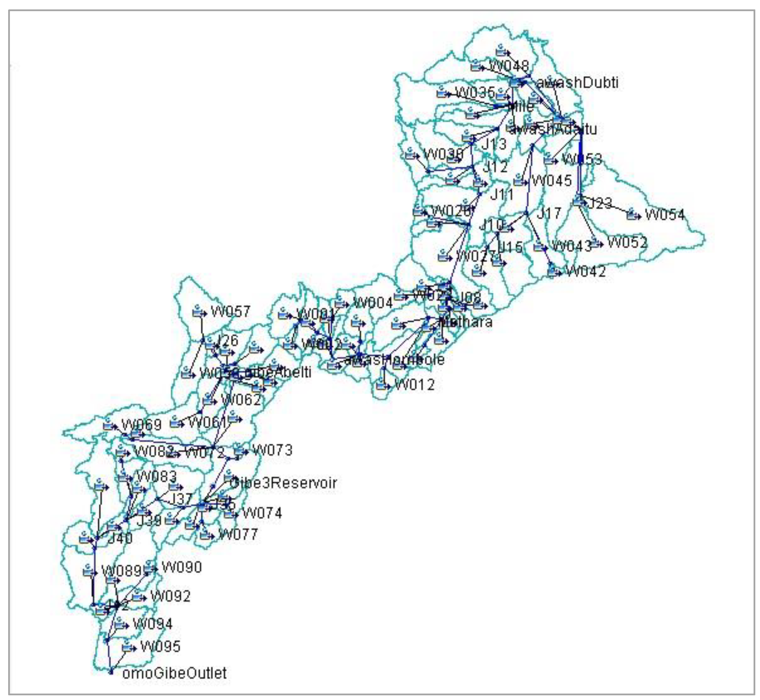
The hydrological model with its new features (HEC-HMS v4.9) was used to produce seasonal floodwater (flow) forecasts in the study basins [37,38]. The project name as an identifier for a hydrologic model that has a basin model, a meteorological model, and control specifications, grid data, and terrain data components was considered before the model was run. Then, to run the basin model, the meteorological model and the control specifications were combined. The basin model and basin features were created in the form of a background map file imported into HEC-HMS from the data derived through HEC-HMS’s GIS application components for model simulation (Figure 3). In the meteorological model, the gridded method and the control specification model were created. The control specifications determine the time shape of the simulation features, such as the starting and ending date and time and the computation time step.
The daily observed rainfall data and river gauge stations for some selected stations were used in a hydrological model to estimate the river runoff and calibrate and verify model results. A daily time step was used for the seasonal forecasting processes based on the time interval of the available observations.

The Loss, Transform, and Routing Methods

In the hydrological model setup, the one-layer deficit and constant loss methods were used for continuous simulation, which changes in moisture content. This method is used in combination with a canopy and surface components to represent interception and capture processes. The modified Clark (ModClark) spatial distributed method [39] was applied in the runoff processes to transform excess precipitation to direct runoff. This method explicitly accounts for variations in travel time to the outlet from all areas of a watershed, and the runoff computations explicitly account for translation and storage. It takes advantage of spatially distributed precipitation, topography, soil, and land cover as input datasets to the model. The radar-based gridded precipitation forecast data was then imported using the HEC-HMS model wizard (or vortex-0.10.22 tool), stored in the HEC-Data Storage System and Visual Utility Engine (HEC-DSSVue) database, and utilized the gridded data of the hydrological model. Finally, the Muskingum-Cunge routing method, which was applied in this study, is a combination of the conservation of mass and the diffusion representation of the conservation of momentum. It uses the equation of motion of continuity with lateral inflow included and the diffusion form of momentum equations to route an inflow hydrograph.
Moreover, the inflow equals outflow initial condition option was adopted, which assumes that the initial outflow is the same as the initial inflow to the reach from upstream (considered as a steady-state initial condition). The Manning’s roughness coefficient [40] value used was 0.035 for the channel and 0.075 for the left and the right river banks. The space-time interval options, Auto DX (space interval), and DT (time interval) method, which maintains numeric stability in the model configuration, and the eight-point shape river cross-section inputs were applied in the river flow routing [41,42]. Furthermore, a recession constant of 0.5 was applied as a baseflow contribution, where most of the model sub-watershed area ranges between 384.7 and 9472.6 km2.

Initial and Boundary Conditions

The initial condition (IC) is introduced at the beginning of the unsteady flow simulation that describes flow changes over time, which represents the runoff at the start of the analysis of heavy rainfall. ICs were defined as a global value used at different calculation nodes for the water depth and reach segments. The data frame used for simulation was the peak flow in the simulation periods, either in hours or days. The time series was then used in the model simulation to maintain a hydraulic energy gradient line of hydrodynamic flow behavior. The boundary condition (BC) is the value of a system input that forces the hydrologic system and causes it to change. In the HEC-HMS model, precipitation served as a BC that causes runoff from a watershed.

2.3.3. Reservoir Water Level Analysis

Reservoirs (or pools) play an important role in flood management strategies. They store floodwater and help to reduce flood risks by attenuating the peak floods and mitigating the intensity of flooding in the downstream reaches [43] and over the flood-prone areas. To reduce a peak flood flow to a target reservoir level, the reservoir provides storage for excess floodwater, which is released gradually at a later time and rate as an operable and controlled release. This limits the release of water during a flood event, thus protecting downstream from the impacts of high flow rates and stages, and providing a method of emptying the pond after the event so that the pond can store the coming runoff. In this analysis and the HEC-HMS model, the Koka reservoir in the Awash basin, and Gibe-3 reservoir in the Omo-Gibe basin were considered to indicate how they change their hydrologic response concerning flood controls and reserving water resources. An Excel spreadsheet was employed for the reservoir water balance analysis, using inflows to and from reservoirs using the water balance equation [44]. Water balance analysis uses the principle of conservation of mass in a closed system [45,46]. It is given as:
P   =   R   +   E   + Δ S Δ t
where P is precipitation, E is evapotranspiration, R is runoff, ΔS is the storage change, and Δt is the time step.
Therefore, the inflow (Qi)-inflows obtained at Awash at Hombole and Mojo River gauging stations and other ungauged [46] tributaries, reservoir storage, outflow (Qo) from the reservoir, losses as evaporation (pan) from the reservoir, and seepage as a function of evaporation were considered. In addition, different analog years were obtained from EMI for the 2021 flood season, and the 2008 analog year and the average year from historical records were considered. Moreover, the normal operating level (NOL) of the Koka reservoir (110.3 m) and the lowest Koka reservoir water level reached about 102.0 m due to the sediments stored in the reservoir from the past decades and were used in the analysis. Similarly, the reservoir information for Gibe-3 was collected and used in the analysis, with a maximum of 892.0 m and minimum of 854.0 m regarding the reservoir water levels. Therefore, this analysis addressed the magnitude of combined inflows, the storage capacity of reservoirs, and the releases without causing flooding downstream when the runoff exceeds the conveyance capacity of the river channel.

2.3.4. Flood Mapping and Semiology

Flood inundation maps are an essential tool for safety and land use planning in flood-prone areas. Flood risk maps are created to show different degrees of risks [47,48] and help to determine flood damages and costs during an emergency and insurance-related information [4]. It is a spatial context of probabilities [49], which is linked to determine the flood inundation extents [50], flood depths, and velocities and estimate the probability of extreme flood events and their negative impacts. In the floodplain, the schematization shows the geometry of the river features, which was developed using a Hydrologic Engineering Center River Analysis System (HEC-RAS) 2-Dimentional mapper. The peak runoff record of the 2006 flood season within the study period (2005–2014) was considered to produce the flood risk maps using the historical flood events and hydrological extremes [50]. Then, the flood inundation maps produced by the model were compared and verified with remote sensing satellite observations [51,52]. The satellite observation inundation maps were accessed from Dartmouth Flood Observation (DFO) service center for Awash basin flood-prone areas [53] and Omo-Gibe basin flood-prone areas [54] to verify the rapid flood inundation maps in the study basins.

2.3.5. Evaluation of Model Performance

The model performance was evaluated using commonly known statistical metrics by comparing the model forecasts and observation values of precipitation and the generated runoff from it. The time-series-based indices: the coefficient of determination (R2), which measures the goodness-of-fit; and the Nash–Sutcliffe efficiency (NSE) coefficient [38], which quantifies how well a model simulation can predict the outcome variable, were applied. In these assessment techniques, if the values are close to 1, this indicates a perfect fit, where the runoff forecasts are compared with observations. The percent of bias (Pbias) measures the average tendency of the simulated data to be larger or smaller than the corresponding observed data [33,34]. The optimal value of Pbias is 0, which indicates the model accuracy, and if it is positive (negative), this indicates underestimation (overestimation) of the model biases. The modified Kling–Gupta efficiency (KGE) [55,56], which is written as a linear transformation of the Euclidian distance of (α, β, r) to the ideal value (1, 1, 1) in a three-dimensional space, was also used. These coefficients of variation were used to avoid the impact of bias on the variability indicator:
R 2 = i = 1 n ( Q s i Q ¯ s ) ( Q o i Q ¯ o ) i = 1 n ( Q s i Q ¯ s ) 2 ( Q o i Q ¯ o ) 2 ; 0 R 2 1
N S E = 1 i = 1 n ( Q o i Q s i ) 2 i = 1 n ( Q o i Q ¯ o ) 2 ; N S E 1
P b i a s = i n ( Q o i Q s i ) i n ( Q o i )
K G E = 1 ( r 1 ) 2 + ( β 1 ) 2 + ( α 1 ) 2  
K G E = 1 ( r 1 ) 2 + ( β 1 ) 2 + ( γ 1 ) 2   ; < K G E < 1
The Pearson correlation coefficient, r, was used to evaluate the error in the shape and timing between the observed and simulated stream flow; Β was used to evaluate the bias between observed and simulated stream flow; α is the ratio between the simulated and observed standard deviations, which was used to evaluate the stream flow variability error; and γ is the ratio between the simulated and observed coefficients of variation (CV), which was used to evaluate the stream flow variability error:
r = c o v ( Q o , Q s ) σ o 2 σ s 2
β = μ s μ o
α = σ s σ o
γ = σ s μ o μ s σ o
where Qsi and Qoi are the simulated and observed values at time step i, respectively; Q ¯ s and Q ¯ o are the corresponding average values, respectively, for simulated and observed variables; “cov” is the covariance between observation and simulation; σ is the standard deviation; and μ is the mean of the observed and simulated flow data.
The HEC-HMS model results were evaluated and compared with the observation. According to the efficiency category [57], if the efficiency values range between 0.40 and 0.55, the model performs satisfactorily; if the value ranges between 0.55 and 0.65, the model performs good; and if the value is above 0.65, it performs very good. In the calibration process, some sensitive parameters in the model basins were considered, and default values for other less sensitive parameters were used. Some of these parameters were the time of concentration, storage coefficient, imperviousness, baseflow-recission, loss/gain-percolation, etc. Thus, the configured and calibrated HEC-HMS model was planned for use in seasonal flow forecasting and early warning systems.
On the other hand, the spatial results of the flood inundation maps from the model produced using the 2-Dimentional HEC-RAS mapper were compared with Earth remote sensing satellite observation images [22]. The images were then exported to vector data (or shapefile) to estimate the flood inundation extents (square meter) in the GIS environment.

3. Results

3.1. Model Performance

3.1.1. Performance of Bias Correction of Rainfall

The bias correction factors determined for the target months of the 2021 flood season were 1.13385 for the month of June, 0.95237 for July, 0.96129 for August, and 1.08784 for September. The R2 values determined for the selected weather stations were 0.95 for Addis Ababa, 0.89 for Methara, 0.99 for Haik, and 0.99 for Jima as presented in Figure 4. Similarly, the performances determined using NSE were 0.94 for Addis Ababa, 0.86 for Methara, 0.93 for Haik, and 0.98 for the Jima weather station.

3.1.2. Performance of the Hydrological Model with Historical Flow-Rate Data

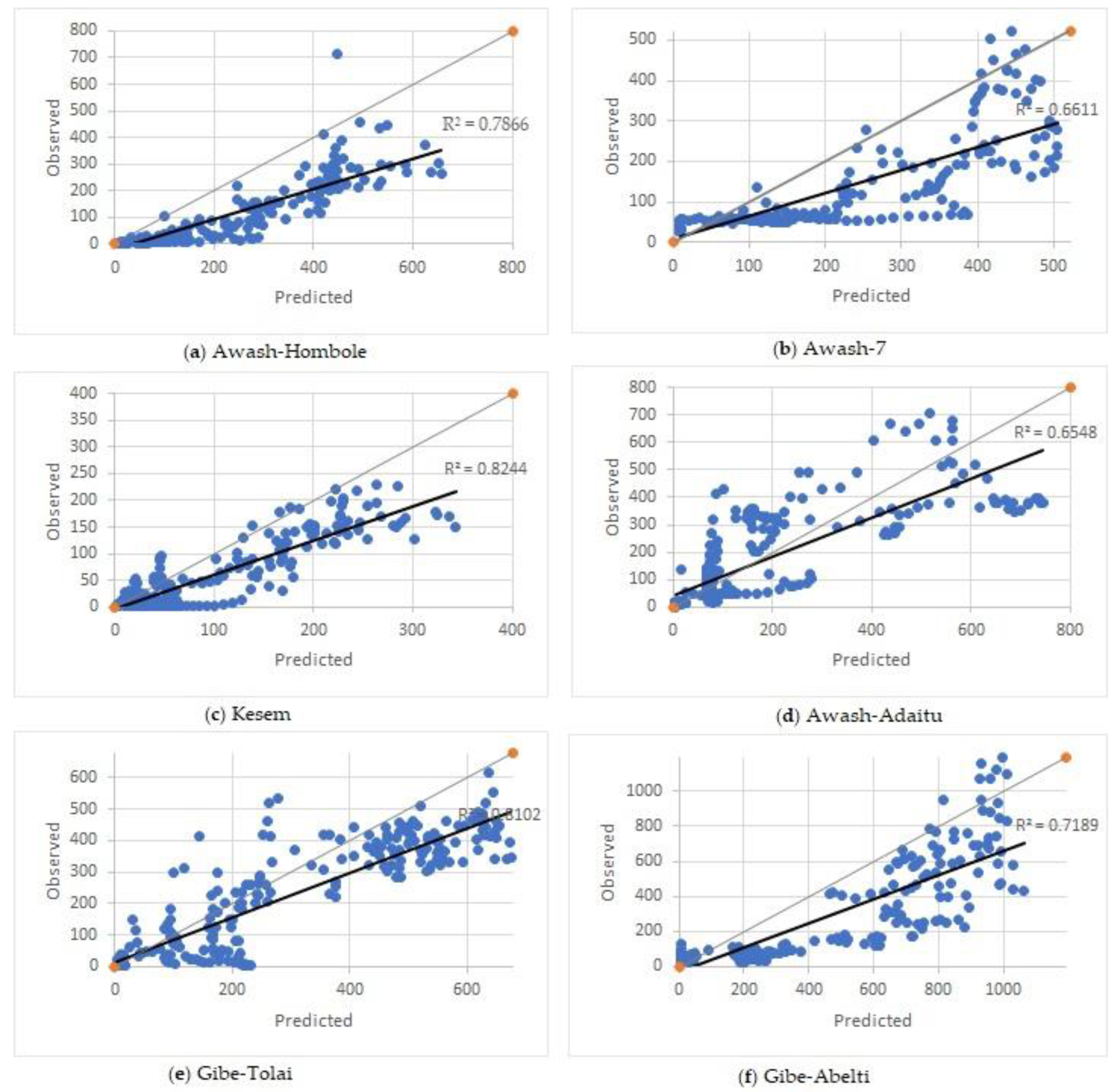
The runoff forecast results from the model were compared with the observed flow rates to evaluate the model’s use of statistical metrics, R2 and NSE, for the selected river gauging stations. The model performed very good as presented in Table 1. The R2 values were 0.79 for Awash-Hombole, 0.66 for Awash-7, 0.82 for Kesem, and 0.65 for the Awash-Adaitu River stations in the Awash basin; and 0.81 for Gibe-Tolai and 0.72 for Gibe-Abelti rivers in the Omo-Gibe basin. The NSE values were obtained for Awash-Kuntire (0.68), Awash-Hombole (0.71), Awash-7 (0.59), and Awash-Adaitu (0.52) rivers in the Awash basin; and Gibe-Toli (0.60) and Gibe-Abelti (0.53) river stations in the Omo-Gibe basin. Similarly, the Pbias and KGE values are also presented in Table 1.
The scatter plots for the selected river gauging stations are also presented in Figure 5, which compares the predicted model results with the observed data and shows very good performance ranges (above 0.65).
Hydrographs for selected river stations from the continuous model simulation were produced using the 2005–2014 observation records. The time series plots for Awash-Hombole, Awash-7, Kesem, and Awash-Adaitu River stations in the Awash basin; and Gibe-Tolai and Gibe-Abelti River stations in the Omo-Gibe basin are presented in Figure 6.

3.1.3. Performance of Flood Maps in Year 2006

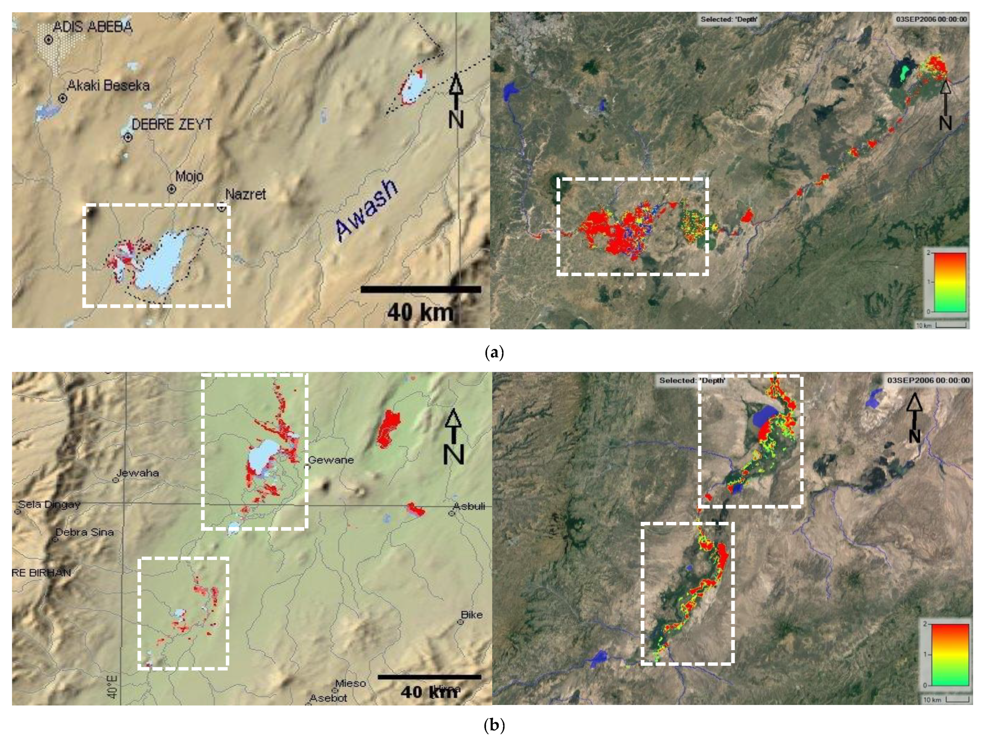
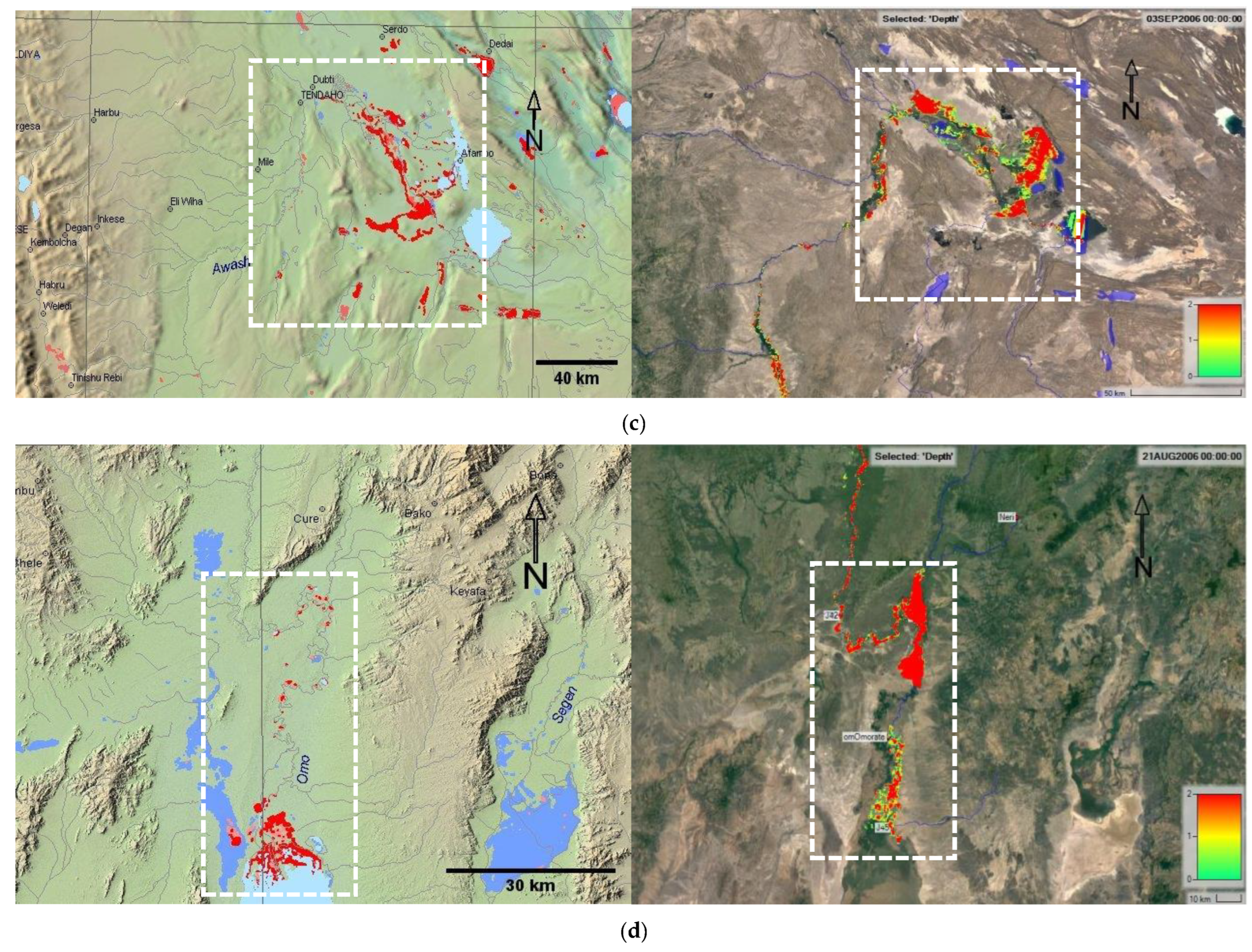
The flood inundation extents from the model were compared with the remotely sensed satellite observation maps captured during the 2006 flood season accessed from DFO for the flood-prone areas of the study basins. Comparative analysis was carried out on the flood inundation results obtained from the model run and the satellite observations on 3 and 21 August 2006 and 3 September 2006 (on similar days and year) as presented in Table 2 and Figure 7. The flood inundation extent over the main flood-prone areas in Awash and Omo-Gibe basins was estimated as 1487.18 km2 (Table 2). This shows that the lower Awash has more flood-impacted areas compared with the middle and upper Awash sub-basins. On the contrary, the upper Awash sub-basin is highly impacted by flooding since more settlements and developments are available than the middle and lower Awash sub-basins. Based on the flood inundation extents produced by the model with respect to the satellite observations (as reference values), the model results were evaluated. The model results are therefore in agreement with the satellite observation images and the model performed very good (Table 2). In this analysis, the lake (natural pool) areas (e.g., lake Koka, 159.52 km2 for upper Awash) were excluded.
The Earth remote sensing satellite images captured on 3 September 2006 for Awash basin (Figure 7a–c) and on 21 August 2006 for Omo-Gibe basin (Figure 7d) were compared with the model results produced by the 2-Dimentional HEC-RAS mapper for the model basins and showed agreement.

3.1.4. Performance of Reservoir Water Levels

A comparative analysis between the runoff forecasts and reservoir water levels was carried out for the 2021 flood season and the observation using the coefficient of determination (R2) and Nash–Sutcliffe efficiency (NSE) as presented in Table 3. Therefore, the R2 values determined for the inflows (water levels) for the Koka reservoir for the 2008 analogue year were 0.92 (0.99) and the NSE values determined for the flows (water levels) were 0.87 (0.95). This showed that the 2021 seasonal floodwater forecasts and the reservoir water levels showed good correlations with the observation of the 2008 analogue year (Table 3).
On the other hand, the 2021 forecasted inflows and reservoir water levels were validated with observations and are presented in Table 4. Therefore, the R2 values determined for inflows (water levels) for the Koka reservoir were 0.97 (0.95) and 0.92 (0.99) for the Gibe-3 reservoir. Likewise, the NSE values for the flows (water levels) for the Koka reservoir were 0.89 (0.88) and 0.91 (0.94) for the Gibe-3 reservoir. This shows that the 2021 seasonal flow forecasts and the reservoir water levels showed good correlations with the observations of 2021 of the same period.

3.2. Rainfall Forecasts at Year 2021

In the model basins, 95 sub-watersheds (w001, w002, …, w095) were produced (Figure 3, Section 2.3.2) in terrain processing to present the contribution of rainfall over each sub-watershed. Based on the analysis, the bias-corrected temporal mean daily precipitation distribution were prepared and are presented in Figure 8.
The spatial distribution of the rainfall over the study basins showed that the upper catchment receives more rainfall, which induces more runoff to trigger flooding (Figure 9). In other words, the rainfall magnitude decreases from the headwater of the model basins to the lowland areas in both time and space.
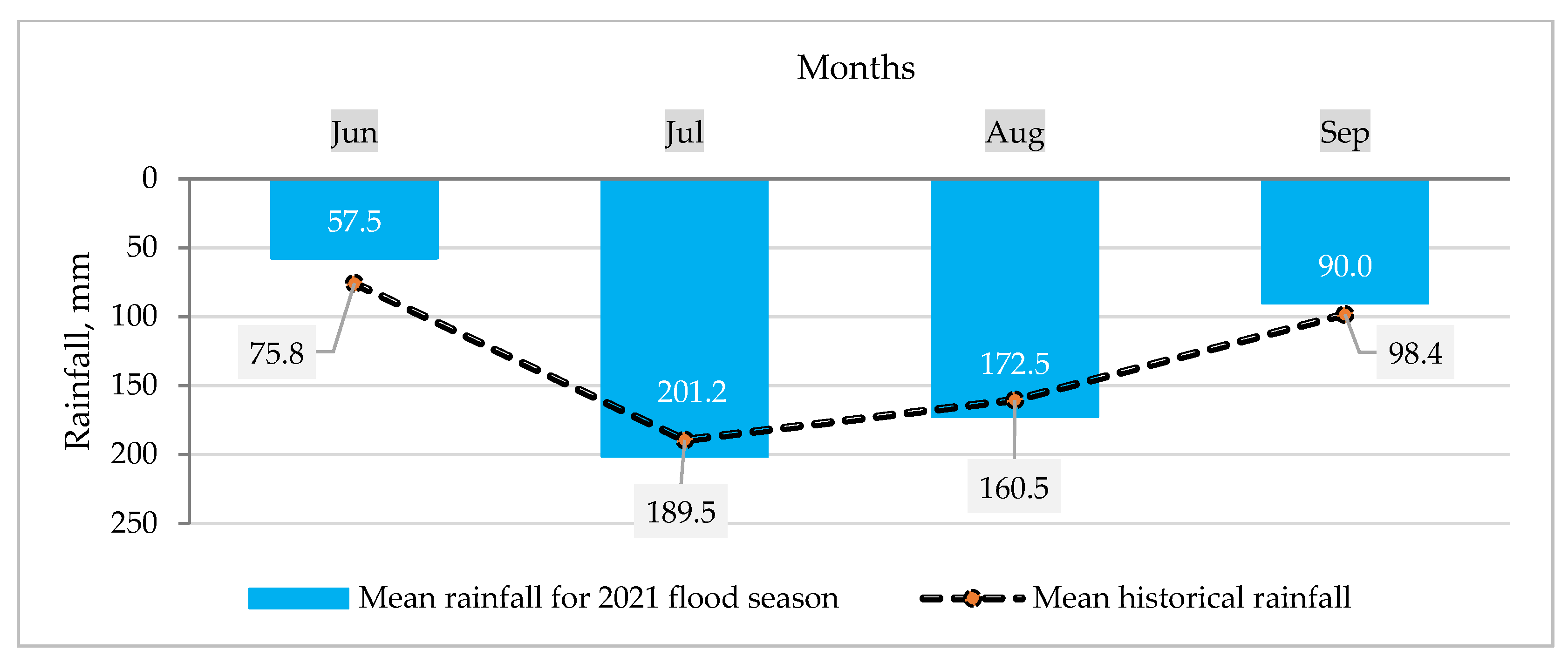
Moreover, the mean accumulated monthly precipitation (Figure 10) showed increasing trends from June (57.5 mm) to July (201.2 mm) and started decreasing after July to August (172.5 mm) and September (90.0 mm). Moreover, the historical mean monthly rainfall is presented in comparison with the 2021 flood season rainfall forecasts (Figure 10). In essence, the rainfall forecasts showed agreement with the underestimated values for June and September and were overestimated for July and August.

3.3. Reservoir Water Level Forecasts

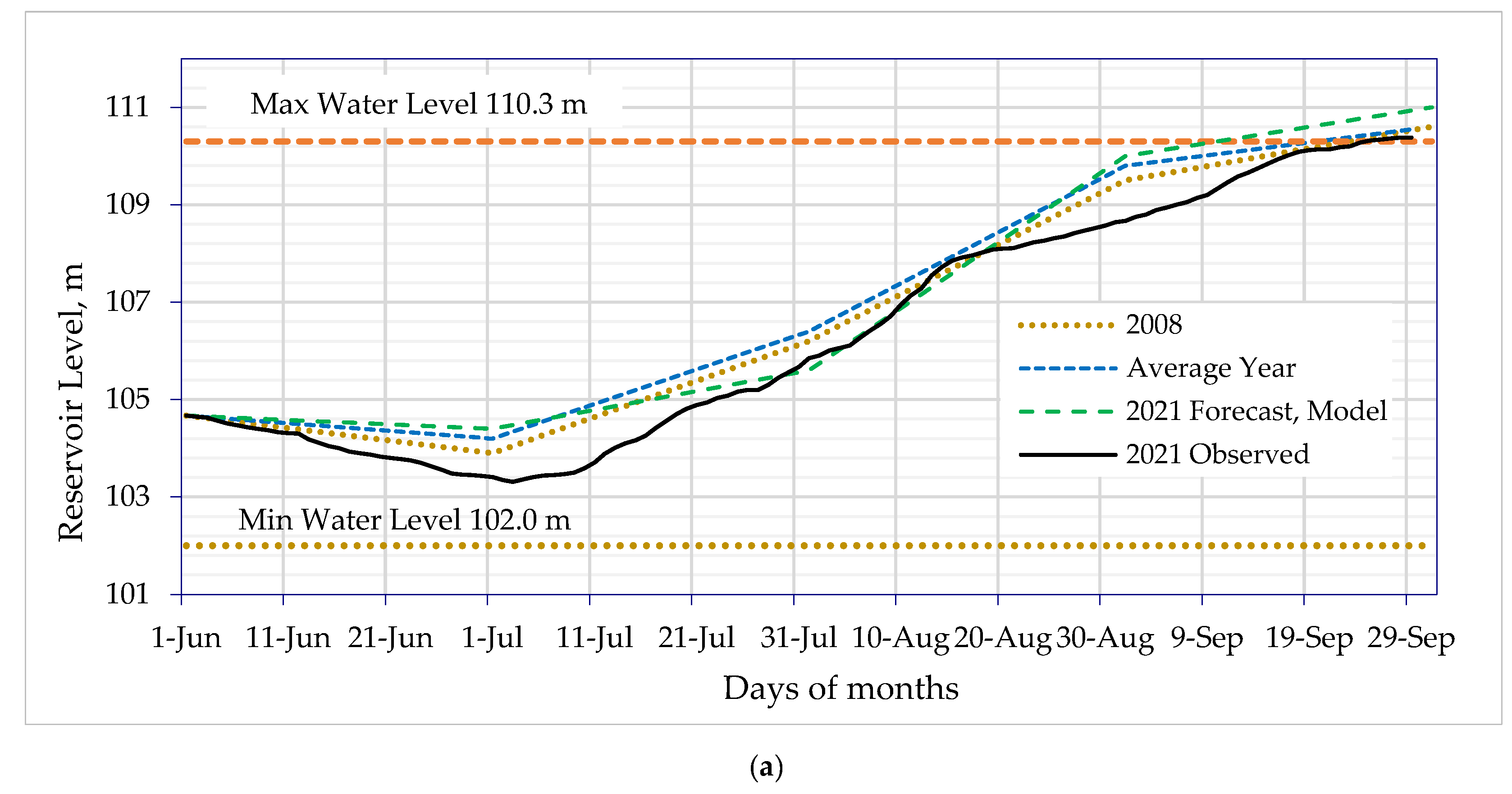
Results showed that the inflows to and outflows from reservoirs, water levels, and storage were estimated for the analog year, the average year, and the model forecasts for the 2021 flood season as presented in Table 5. The seasonal floodwater forecasts of Awash-Hombole and Mojo rivers are major water resources for the Koka reservoir (Figure 11a). If the reservoir water level of Koka reached 109 m and above, water release from the reservoir can be identified based on the peak floodwater entering the reservoir. Similarly, the river flows from Gojeb-Shebe and Gibe-Abelti with other small gauged and ungauged tributaries are the major water resources contributing to the Gibe-3 reservoir (Figure 11b). In general, inflow forecasts of water entering and leaving these reservoirs may result in flooding over flood-prone areas downstream, river banks, and reservoirs, which maintain excess floodwater for dry period uses.
The reservoir water level was 104.67 m on June 1 with storage of 294.34 Mm3 at Koka and 865.71 m with 10,056.5 Mm3 of storage at Gibe-3 reservoir. The flow forecast values, water levels, and storage at the end of each month for the target years were estimated and are presented in Table 5. In the table, for instance, the model estimated and observed Koka reservoir water levels at the end of September reached 110.60 and 110.36 m, respectively. The estimated and observed Gibe-3 reservoir water levels reached 892.00 and 891.39 m, respectively, at the end of September.
The water levels forecasts for the 2021 flood season were also plotted together with the 2008 analog year, the average year, together with the observed data. The water level forecasts of Koka reservoir (Figure 11a) and Gibe-3 reservoir (Figure 11b) were in agreement with the 2008 analog year, average year, and observed data of the target 2021 flood season.
Based on the monthly flow forecasts to the reservoirs and the storage, the decision to release can be made with some lead time to supplement flood monitoring systems. In this case, the relational plans between inflow forecasts to reservoirs, the water levels in the reservoir, and measured releases from reservoirs are important components to consider. If this forecast information is not produced in time nor ready for use, there is a chance of probable flood-related impacts downstream and meager reservation of water supply during dry periods. In general, reservoirs are used to maintain water, maximize water use benefits, and mitigate impacts from hydrologic extremes, which are excess (or shortage) water resources used to meet planned objectives without affecting the environmental water requirements.

4. Discussion

A seasonal flow (floodwater) forecasting system has not been addressed in the study basins to monitor and reduce flood risks and use the benefits of excess floodwater for water resource planning and development. There is no well-established flood forecasting and monitoring infrastructure in the study basins; instead, traditional techniques are exercised. This involves data and information collected from river stations and reservoir water levels [58] and the use of manual interventions, which is ineffective in transferring data to the forecasting center. In addition, these collection techniques delay the preparation and dissemination of flood forecasting and early warnings to decision-makers and local communities. These further delays coordinated flood early warning information, which may result in flooding impacts and damages.
The excess floodwater over the catchments of the study basins induced from heavy rainfall in upland areas causes riverine floodings downstream. In addition, the vegetation cover and soil affect the amount of runoff produced in the catchment and cause flooding. In the target basins, for instance, the changes in catchment characteristics can modify the features of river flooding, which requires planning for sustainable development and flood risk management systems [59,60]. The impacts of flood inundations [61,62] comes from river flooding, which occurs when the volume of river runoff exceeds the river conveyance capacities. In this case, the river rises, and its fall may take periods that last weeks or month. In addition, the failure of reservoir operations (Koka and Gibe-3 reservoirs) in flood control upstream can lead to fluvial flooding and inundation in flood-prone areas.
In previous studies on seasonal floodwater forecasts, results indicated that early forecast information is used in water resource planning and development strategies and flood risk mitigation [63,64]. Excess floodwater forecasts, for instance, need to possess technical guidance on relevant and specific aspects to maintain excess floodwater in reservoirs and support flood management practitioners [65]. To mitigate flooding impacts using reservoir operation strategies, different operation schemes have been proposed by researchers to control target reservoir storages [66] and flood resilience and management activities [67]. In this research, results showed that peak river flow can be minimized using the proposed arrangements. Nevertheless, the investigation did not use seasonal forecasts at the seasonal scale, which are useful for reservoirs’ water management and operation [68,69] and multi-purpose reservoir operations [70]. According to the literature, flood reduction measures range from traditional (or manual) to technology intervention monitoring systems and reservoir water monitoring to complement flood control mechanisms. In this study, Earth remote sensing products and GIS tools were used to produce flood forecasting information and flood risk maps to reduce flooding impact and damage [70,71].
In essence, the seasonal flood forecasting system will provide practical flood monitoring actions to reduce flood impacts in the study basins and excess floodwater management in the Koka and Gibe-3 reservoirs. In order to provide timely flood forecasting and early warnings, it is important to play a role in flood management systems through scientific and technical approaches. In various literature, monitoring of the impacts of riverine flooding and the flood risk management tool is considered [71]. In some cases, the effectiveness of flood risk management systems can be reduced through the variability of flooding and incompatibility of different approaches. In this case, a web-based flood tool can be used to convey the forecasting products and dissemination facilities [8] to inform decision-makers regarding reservoir water monitoring and reduce flooding impacts downstream. The flood management tool supports the conveyance of forecast products and early warnings.
In the present study, the seasonal floodwater forecast system showed many benefits, including the preservation of excess floodwater in reservoirs for future uses, complementing the flood control system. Nevertheless, there are some limitations, such as (1) the time needed to forecast products and for the mode of dissemination planned to deliver early warnings to create awareness and familiarize decision-makers and users; (2) the forecast models for the domain basins are stand-alone operated using satellite-driven datasets, which means the forecast products need to be placed in a dedicated location that is accessible by users; (3) automation and integration of the model input datasets from satellites, the forecasting model runs, and the flood tool requires investment and operational resources, for instance, hosting the flood management tool and future running of the forecasting models on cloud-based infrastructure; and (4) the absence of well-organized institutional arrangements for the national flood response plan, which aims to provide directions and guidance to serve for monitoring, preparedness, and emergency precautionary measures. In this case, the implementation of the flood management tool shall present a surge in resilience against flooding impacts and future water resource monitoring systems, and (5) it requires the development of reservoir rule curves to monitor reservoir water resources from excess floodwater that enters and is released from reservoirs. In general, addressing the above limitations, future study will further improve the seasonal forecasting systems, dissemination facilities to support the decision-making processes in future water resources planning and management strategies, mitigate the negative impacts from flooding in the study basins, and upscale its services to the national level.

5. Conclusions

In extreme hydrological events, flooding is one of the major sources of floodwater and poses major threats to people, socio-economics, and the environment in flood-prone areas when it is excessive. In the past, extreme flooding events in Ethiopia, such as the 1996, 2006, 2016, and 2020 flood seasons, were sources of excess floodwater and impacted people and destroyed their homes and businesses. The present study, therefore, developed a seasonal flow forecasting system to estimate the floodwater availabilities and to reduce recurrent flooding impacts in the Awash and Omo-Gibe basins where flooding impacts are an issue. The data used were the bias-corrected seasonal precipitation and temperature forecasts accessed from ClimateSERV (0.5 deg) and the observed rainfall and discharge data for model calibration and verification of the model results. The methods utilized were the hydrological model (HEC-HMS) and hydrodynamic model (HEC-RAS) with GIS features to estimate runoff forecasts and reservoir water balance analysis to estimate the reservoirs’ water levels for the 2021 flood season as a case study.
Some of the forecast results were the rainfall and runoff forecasts at different gauged and ungauged locations, reservoir water levels, and reservoir storages. In the model evaluation, the coefficient of determination (R2), Nash–Sutcliffe efficiency (NSE), percent of bias (Pbias), and Kling–Gupta efficiency (KGE) were applied in addition to plots. In this case, the R2 and NSE values for selected river gauging stations were obtained and ranged from 0.60 for Gibe-Abelti to 0.79 for Awash-Hombole rivers. The Pbias and KGE values were also obtained. The R2 values for the Koka and Gibe-3 reservoir inflows (water levels) were 0.97 (0.95) and 0.93 (0.99), and the NSE values were 0.90 (0.88) and 0.92 (0.95), respectively. Based on the inflow forecasts, the estimated water levels (storages in Mm3) for the Koka reservoir were 103.3 m (159.09) for June, 105.4 m (386.38) for July, 108.8 m (900.94) for August, and 111.0 m (1467.58) for September. Likewise, the estimated water levels (storage) for the Gibe-3 reservoir were 862.1 (9546.9), 871.1 (10,937.3), 890.0 (13,530.5), and 890.8 m (13,638.5) for each month, respectively. Moreover, the flood inundation extents obtained from remote sensing satellite observation were compared with the model results for the main flood-prone areas for the 2006 flood event. The comparative results indicated agreement with the flood inundation extent and the model performed very good. In the analysis, the likelihood of flooding impacting the upper Awash was higher than the middle and lower Awash sub-basins where there are dense settlements and more developed infrastructure.
In summary, the in-situ satellite-driven precipitation and temperature seasonal forecast data were used to estimate the excess floodwater retained in reservoirs for future water requirements, complementing the flood monitoring system. In essence, the amount of water to be stored in and released from the reservoir can be decided based on inflows and future water use requirements and to protect flood-prone communities, properties, and infrastructure from the likelihood of flooding impacting downstream. In general, the seasonal floodwater forecasting system can inform decision-makers on future water resource planning and management and flood monitoring and early warning systems to reduce flooding impacts. In the future, the present study can be improved in its operational functionalities and upscale its services from the basin level to the national level.

Author Contributions

Research concepts, methodology, and analysis, S.M.W. and B.B.K.; guiding the formal analysis and validation of the final results, B.B.K. and A.M.M. All authors have read and agreed to the published version of the manuscript.

Funding

This research received no external funding.

Data Availability Statement

Not applicable.

Acknowledgments

The authors acknowledge the Ethiopia Meteorological Institute (EMI) and the Ministry of Water and Energy (MOWE) of Ethiopia, the Water and Land Resources Center (WLRC), and ClimateSERV for the datasets used in this study.

Conflicts of Interest

The authors declare there is no conflict of interest.

References

  1. Siam, M.S.; Eltahir, E.A.B. Explaining and forecasting interannual variability in the flow of the Nile River. Hydrol. Earth Syst. Sci. 2015, 19, 1181–1192. [Google Scholar] [CrossRef]
  2. Slater, L.; Villarini, G.; Bradley, A. Evaluation of the skill of North-American Multi-Model Ensemble (NMME) Global Climate Models in predicting average and extreme precipitation and temperature over the continental USA. Clim. Dyn. 2019, 53, 7381–7396. [Google Scholar] [CrossRef]
  3. Romanescu, G.; Mihu-Pintilie, A.; Stoleriu, C.C.; Carboni, D.; Paveluc, L.E.; Cimpianu, C.I. A Comparative Analysis of Exceptional Flood Events in the Context of Heavy Rains in the Summer of 2010: Siret Basin (NE Romania) Case Study. Water 2018, 10, 216. [Google Scholar] [CrossRef]
  4. Di Baldassarre, G.; Viglione, A.; Carr, G.; Kuil, L.; Salinas, J.L.; Blöschl, G. Socio-hydrology: Conceptualising human-flood interactions. Hydrol. Earth Syst. Sci. 2013, 17, 3295–3303. [Google Scholar] [CrossRef]
  5. de Perez, E.C.; Stephens, E.; Bischiniotis, K.; van Aalst, M.; van den Hurk, B.; Mason, S.; Nissan, H.; Pappenberger, F. Should seasonal rainfall forecasts be used for flood preparedness. Hydrol. Earth Syst. Sci. 2017, 21, 4517–4524. [Google Scholar] [CrossRef]
  6. Korecha, D.; Sorteberg, A. Validation of operational seasonal rainfall forecast in Ethiopia. Water Resour. Res. 2013, 49, 7681–7697. [Google Scholar] [CrossRef]
  7. 2016 Ethiopia Flood. Deadly Floods Hit Ethiopia. Wikipedia. 6 April 2016. Available online: https://en.wikipedia.org/wiki/2016_Ethiopia_flood/ (accessed on 25 May 2022).
  8. Woldegebrael, S.M.; Kidanewold, B.B.; Melesse, A.M. Development and Evaluation of a Web-Based and Interactive Flood Management Tool for Awash and Omo-Gibe Basins, Ethiopia. Water 2022, 14, 2195. [Google Scholar] [CrossRef]
  9. Byrne, M.P.; Pendergrass, A.G.; Rapp, A.D.; Wodzicki, K.R. Response of the Intertropical Convergence Zone to Climate Change: Location, Width, and Strength. Curr. Clim. Chang. Rep. 2018, 4, 355–370. [Google Scholar] [CrossRef]
  10. Suzuki, T. Seasonal variation of the ITCZ and its characteristics over Central Africa. Theor. Appl. Climatol. 2010, 103, 39–60. [Google Scholar] [CrossRef]
  11. Nicholson, S.E. The predictability of rainfall over the Greater Horn of Africa. Part I. Prediction of seasonal rainfall. J. Hydrometeor. 2014, 15, 1011–1027. [Google Scholar] [CrossRef]
  12. Berhanu, B.K.; Seleshi, Y.; Demisse, S.S.; Assefa, A.M. Bias correction and characterization of climate forecast system re-analysis daily precipitation in Ethiopia using fuzzy overlay. Meteorol. Appl. 2016, 23, 230–243. [Google Scholar] [CrossRef]
  13. NMSA. Climatic & Agroclimatic Resources of Ethiopia; Meteorological Research Report Series; National Meteorological Services Agency: Addis Ababa, Ethiopia, 1996; Volume 1. [Google Scholar]
  14. Weisheimer, A.; Palmer, T.N. On the reliability of seasonal climate forecasts. J. R. Soc. Interface 2014, 11, 20131162. [Google Scholar] [CrossRef] [PubMed]
  15. Gain, A.; Apel, H.; Renaud, F.; Giupponi, C. Thresholds of hydrologic flow regime of a river and investigation of climate change impact—The case of the Lower Brahmaputra River Basin. Clim. Chang. 2013, 120, 463–475. [Google Scholar] [CrossRef]
  16. Food and Agricultural Organization of the United Nations. Soil Maps and Databases. Available online: https://www.fao.org/soils-portal/data-hub/soil-maps-and-databases/ (accessed on 20 February 2021).
  17. ClimateSERV. SERVIR Global. Available online: https://climateserv.servirglobal.net/ (accessed on 31 May 2021).
  18. Becker, E.; Van den Dool, H.; Zhang, Q. Predictability and forecast skill in NMME. J. Clim. 2014, 27, 5891–5906. [Google Scholar] [CrossRef]
  19. Woldegebrael, S.M.; Berhanu, B.; Zaitchik, B.; Melesse, A.M. Rainfall and Flood Event Interrelationship—A Case Study of Awash and Omo-Gibe Basins, Ethiopia. Int. J. Sci. Eng. Res. 2020, 11, 332–343. [Google Scholar]
  20. Hawker, L.; Bates, P.; Neal, J.; Rougier, J. Perspectives on Digital Elevation Model (DEM) Simulation for Flood Modeling in the Absence of a High-Accuracy Open Access Global DEM. Front. Earth Sci. 2018, 6, 233. [Google Scholar] [CrossRef]
  21. Samela, C.; Manfreda, S.; Nardi, F.; Grimaldi, S.; Roth, G.; Sole, A. DEM-based Approaches for the Identification of Flood Prone Areas. In Geophysical Research Abstracts; EGU General Assembly: Vienna, Austria, 2013; Volume 15, pp. 2013–8177. [Google Scholar]
  22. Degiorgis, M.; Gnecco, G.; Gorni, S.; Roth, G.; Sanguineti, M.; Taramasso, A.C. Classifiers for the detection of flood-prone areas using remotely sensed elevation data. J. Hydrol. 2012, 470–471, 302–315. [Google Scholar] [CrossRef]
  23. Zheng, L.; Xu, J.; Chen, Y.; Wu, Z. Increasing Streamflow in Poor Vegetated Mountain Basins Induced by Greening of Underlying Surface. Remote Sens. 2022, 14, 3223. [Google Scholar] [CrossRef]
  24. Lane, S.N.; Milledge, D.G. Impacts of upland open drains upon runoff generation: A numerical assessment of catchment-scale impacts. Hydrol. Processes 2013, 27, 1701–1726. [Google Scholar] [CrossRef]
  25. Berhanu, B.K.; Assefa, M.M.; Seleshi, Y. GIS-Based Hydrological Zones and Soil Geodatabase of Ethiopia, Catena; Elsevier: Amsterdam, The Netherlands, 2013; Volume 104, pp. 21–31. [Google Scholar]
  26. Dile, Y.T.; Berndtsson, R.; Setegn, S.G. Hydrological Response to Climate Change for Gilgel Abay River, in the Lake Tana Basin—Upper Blue Nile Basin of Ethiopia. PLoS ONE 2013, 8, e79296. [Google Scholar] [CrossRef]
  27. Ahmed, K.F.; Wang, G.; Silander, J.; Wilson, A.M.; Allen, J.M.; Horton, R.; Anyah, R. Statistical downscaling and bias correction of climate model outputs for climate change impact assessment in the US northeast. Glob. Planet. Change 2013, 100, 320–332. [Google Scholar] [CrossRef]
  28. Mehrotra, R.; Sharma, A. An improved standardization procedure to remove systematic low frequency variability biases in GCM simulations. Water Resour. Res. 2012, 48, W12601. [Google Scholar] [CrossRef]
  29. Turco, M.; Llasat, M.C.; Herrera, S.; Gutiérrez, J.M. Bias correction and downscaling of future rcm precipitation projections using a mos-analog technique. J. Geophys. Res. Atmos. 2017, 122, 2631–2648. [Google Scholar] [CrossRef]
  30. Chen, J.; Brissette, F.P.; Chaumont, D.; Braun, M. Performance and uncertainty evaluation of empirical downscaling methods in quantifying the climate change impacts on hydrology over two North American river basins. J. Hydrol. 2013, 479, 200–214. [Google Scholar] [CrossRef]
  31. Hagemann, S.; Chen, C.; Haerter, J.O.; Heinke, J.; Gerten, D.; Piani, C. Impact of statistical bias correction on the projected hydrological changes obtained from three GCMs and two hydrology models. J. Hydrometeorol. 2011, 12, 556–578. [Google Scholar] [CrossRef]
  32. Fang, G.; Yang, J.; Chen, Y.; Zammit, C. Comparing bias correction methods in downscaling meteorological variables for a hydrologic impact study in an arid area in China. Hydrol. Earth Syst. Sci. 2015, 19, 2547–2559. [Google Scholar] [CrossRef]
  33. Luo, M.; Liu, T.; Meng, F.; Duan, Y.; Frankl, A.; Bao, A.; De Maeyer, P. Comparing Bias Correction Methods Used in Downscaling Precipitation and Temperature from Regional Climate Models: A Case Study from the Kaidu River Basin in Western China. Water 2018, 10, 1046. [Google Scholar] [CrossRef]
  34. Lafon, T.; Dadson, S.; Buys, G.; Prudhomme, C. Bias correction of daily precipitation simulated by a regional climate model: A comparison of methods. Int. J. Climatol. 2013, 33, 1367–1381. [Google Scholar] [CrossRef]
  35. Verdin, A.; Funk, C.; Rajagopalan, B.; Kleiber, W. Kriging and Local Polynomial Methods for Blending Satellite-Derived and Gauge Precipitation Estimates to Support Hydrologic Early Warning Systems. IEEE Trans. Geosci. Remote Sens. 2016, 54, 2552–2562. [Google Scholar] [CrossRef]
  36. Yang, X.; Xie, X.; Liu, D.L.; Ji, F.; Wang, L. Spatial Interpolation of Daily Rainfall Data for Local Climate Impact Assessment over the Greater Sydney Region. Adv. Meteorol. 2015, 2015, 563629. [Google Scholar] [CrossRef]
  37. Steyerberg, E.W.; Vickers, A.J.; Cook, N.R.; Gerds, T.; Gonen, M.; Obuchowski, N.; Pencina, M.J.; Kattan, M.W. Assessing the performance of prediction models: A framework for traditional and novel measures. Epidemiology 2010, 21, 128–138. Available online: http://www.jstor.org/stable/25662818 (accessed on 4 September 2022). [CrossRef] [PubMed]
  38. Nash, J.E.; Sutcliffe, J.V. River flow forecasting through conceptual models’ part I-A discussion of principles. J. Hydrol. 1970, 10, 282–290. [Google Scholar] [CrossRef]
  39. Gharib, M.; Motamedvaziri, B.; Ghermezcheshmeh, B.; Ahmadi, H. Evaluation of ModClark model for simulating rainfall-runoff in Tangrah watershed, Iran. Appl. Ecol. Environ. Res. 2018, 16, 1053–1068. [Google Scholar] [CrossRef]
  40. Phillips, J.V.; Tadayon, S. Selection of Manning’s Roughness Coefficient for Natural and Constructed Vegetated and Non-Vegetated Channels, and Vegetation Maintenance Plan Guidelines for Vegetated Channels in Central Arizona; U.S. G.S. Scientific Investigations Report 2006–5108; US Geological Survey: Reston, VA, USA, 2006; 41p.
  41. Martins, O.; Kamar, O. Application of Basic Excel Programming to Linear Muskingum Model for Open Channel Routing. J. Civ. Environ. Res. 2017, 9, 39–54. [Google Scholar]
  42. Samani, H.M.; Shamsipour, G.A. Hydrologic flood routing in branched river systems via nonlinear optimization. J. Hydraul. Res. 2010, 2004, 55–59. [Google Scholar] [CrossRef]
  43. McCuen, R.H. Downstream effects of stormwater management basins. J. Hydraul. Div. 1979, 105, 1343–1356. [Google Scholar] [CrossRef]
  44. Kim, D.G.; Kim, S.J.; Ahn, T.J. Wetland Construction: Flood Control and Water Balance Analysis. Environ. Eng. Res. 2010, 15, 197–205. [Google Scholar] [CrossRef]
  45. Bock, A.R.; Hay, L.E.; Markstrom, S.L.; Emmerich, C.; Talbert, M. The U.S. Geological Survey Monthly Water Balance Model Futures Portal; U.S. Geological Survey Open-File Report 2016–1212; US Geological Survey: Reston, VA, USA, 2017; 21p. [CrossRef]
  46. Pattison, I.; Lane, S.N.; Hardy, R.J.; Reaney, S.M. The role of tributary relative timing and sequencing in controlling large floods. Water Resour. Res. 2014, 50, 5444–5458. [Google Scholar] [CrossRef]
  47. Tarekegn, T.H.; Haile, A.T.; Rientjes, T.; Reggiani, P.; Alkema, D. Assessment of an ASTER-generated DEM for 2D hydrodynamic flood modeling. Int. J. Appl. Earth Obs. Geoinf. 2010, 12, 457–465. [Google Scholar] [CrossRef]
  48. Tate, E.C.; Maidment, D.R. Floodplain Mapping Using HEC-RAS and ArcView GIS; University of Texas at Austin: Austin, TX, USA, 1999. [Google Scholar] [CrossRef]
  49. Dorner, W.; Schrenk, C.; Spachinger, K.; Metzka, R. Flood risk management plan-Relevance of the hydrological behavior of a catchment. In Proceedings of the XXIII Conference of the Danube Countries on the Hydrological Forecasting and Hydrological Bases of Water Management CD-ROM, Belgrade, Serbia, 28–31 August 2006; Bruck, S., Petkovic, T., Eds.; ICPDR—International Commission for the Protection of the Danube River: Vienna, Austria, 2006. [Google Scholar] [CrossRef]
  50. Mamo, S.; Berhanu, B.; Melesse, A.M. Historical flood events and hydrological extremes in Ethiopia. In Extreme Hydrology and Climate Variability; Elsevier: Amsterdam, The Netherlands, 2019; pp. 379–384. [Google Scholar] [CrossRef]
  51. Mandl, D.; Frye, S.; Cappelaere, P.; Handy, M.; Policelli, F.; Katjizeu, M.; Van Langenhove, G.; Aube, G.; Saulnier, J.F.; Sohlberg, R.; et al. Use of the Earth Observing One (EO-1) Satellite for the Namibia Sensorweb Flood Early Warning Pilot. IEEE J. Sel. Top. Appl. Earth Obs. Remote Sens. 2013, 6, 298–308. [Google Scholar] [CrossRef]
  52. Fluet-Chouinard, E.; Lehner, B.; Rebelo, L.M.; Papa, F.; Hamilton, S.K. Development of a global inundation map at high spatial resolution from topographic downscaling of coarse-scale remote sensing data. Remote Sens. Environ. 2015, 158, 348–361. [Google Scholar] [CrossRef]
  53. Flood Observatory. 2006-174 Nile. Available online: https://floodobservatory.colorado.edu/2006174Nile.html (accessed on 17 December 2018).
  54. Flood Observatory. Images, 2006–2170 Omo Delta. Available online: https://floodobservatory.colorado.edu/images/2006170OmoDelta.jpg (accessed on 17 December 2018).
  55. Kling, H.; Fuchs, M.; Paulin, M. Runoff conditions in the upper Danube basin under an ensemble of climate change scenarios. J. Hydrol. 2012, 424–425, 264–277. [Google Scholar] [CrossRef]
  56. Gupta, H.V.; Kling, H.; Yilmaz, K.K.; Martinez, G.F. Decomposition of the mean squared error and NSE performance criteria: Implications for improving hydrological modelling. J. Hydrol. 2009, 377, 80–91. [Google Scholar] [CrossRef]
  57. Moriasi, D.N.; Arnold, J.G.; van Liew, M.W.; Bingner, R.L.; Harmel, R.D.; Veith, T.L. Model Evaluation Guidelines for Systematic Quantification of Accuracy in Watershed Simulations. Trans. ASABE 2007, 50, 885–900. [Google Scholar] [CrossRef]
  58. Liu, P.; Li, L.; Guo, S.; Xiong, L.; Zhang, W.; Zhang, J.; Xu, C. Optimal design of seasonal flood limited water levels and its application for the Three Gorges Reservoir. J. Hydrol. 2015, 527, 1045–1053. [Google Scholar] [CrossRef]
  59. Guan, D.J.; Li, H.F.; Inohae, T.; Su, W.C.; Nagaie, T.; Hokao, K. Modeling urban land-use change by the integration of cellular automaton and Markov model. Ecol. Model. 2011, 222, 3761–3772. [Google Scholar] [CrossRef]
  60. Baulies, X.; Szejwach, G. LUCC Data Requirements Workshop. In Lucc Data Requirements Workshop: Survey of Needs, Gaps and Priorities on Data for Land-Use; Institut Cartogràfic de Catalunya: Barcelona, Spain, 1998. [Google Scholar]
  61. Conway, D. The climate and hydrology of the Upper Blue Nile River. Geograph. J. 2000, 166, 49–62. [Google Scholar] [CrossRef]
  62. Alemu, W.G.; Dagnachew, L.B. Flood hazard and risk assessment in Fogera Wereda using GIS & remote sensing. In Nile River Basin Hydrology; Melesse, A.M., Ed.; Springer: Dordrecht, The Netherlands, 2011. [Google Scholar]
  63. Cislaghi, A.; Masseroni, D.; Massari, C.; Camici, S.; Brocca, L. Combining a rainfall–runoff model and a regionalization approach for flood and water resource assessment in the western Po Valley, Italy. Hydrol. Sci. J. 2020, 65, 348–370. [Google Scholar] [CrossRef]
  64. De Bruijn, K.M.; Maran, C.; Zygnerski, M.; Jurado, J.; Burzel, A.; Jeuken, C.; Obeysekera, J. Flood Resilience of Critical Infrastructure: Approach and Method Applied to Fort Lauderdale, Florida. Water 2019, 11, 517. [Google Scholar] [CrossRef]
  65. Song, Y.; Park, Y.; Lee, J.; Park, M.; Song, Y. Flood Forecasting and Warning System Structures: Procedure and Application to a Small Urban Stream in South Korea. Water 2019, 11, 1571. [Google Scholar] [CrossRef]
  66. Mateo, C.M.; Hanasaki, N.; Komori, D.; Tanaka, K.; Kiguchi, M.; Champathong, A.; Sukhapunnaphan, T.; Yamazaki, D.; Oki, T. Assessing the impacts of reservoir operation to floodplain inundation by combining hydrological, reservoir management, and hydrodynamic models. Water Resour. Res. 2014, 50, 7245–7266. [Google Scholar] [CrossRef]
  67. Tasseff, B.; Bent, R.; Van Hentenryck, P. Optimization of Structural Flood Mitigation Strategies. Water Resour. Res. 2019, 55, 1490–1509. [Google Scholar] [CrossRef]
  68. Lucatero, D.; Madsen, H.; Refsgaard, J.C.; Kidmose, J.; Jensen, K.H. Seasonal streamflow forecasts in the Ahlergaarde catchment, Denmark: The effect of preprocessing and post-processing on skill and statistical consistency. Hydrol. Earth Syst. Sci. 2018, 22, 3601–3617. [Google Scholar] [CrossRef]
  69. Wongnarin, K.; Sayaka, Y.; Shinjiro, K. Use of Seasonal Streamflow Forecasts for Flood Mitigation with Adaptive Reservoir Operation: A Case Study of the Chao Phraya River Basin, Thailand, in 2011. Water 2020, 12, 3210. [Google Scholar] [CrossRef]
  70. Ehteram, M.; Mousavi, S.-F.; Karami, H.; Farzin, S.; Emami, M.; Othman, F.; Amini, Z.; Kisi, O.; El-Shafie, A. Fast convergence optimization model for single and multi-purposes reservoirs using hybrid algorithm. Adv. Eng. Inform. 2017, 32, 287–298. [Google Scholar] [CrossRef]
  71. Argaz, A.; Ouahman, B.; Darkaoui, A.; Bikhtar, H.; Ayouch, E.; Lazaar, R. Flood Hazard Mapping Using remote sensing and GIS Tools: A case study of Souss Watershed. J. Mater. Environ. Sci. 2019, 10, 170–181. [Google Scholar]
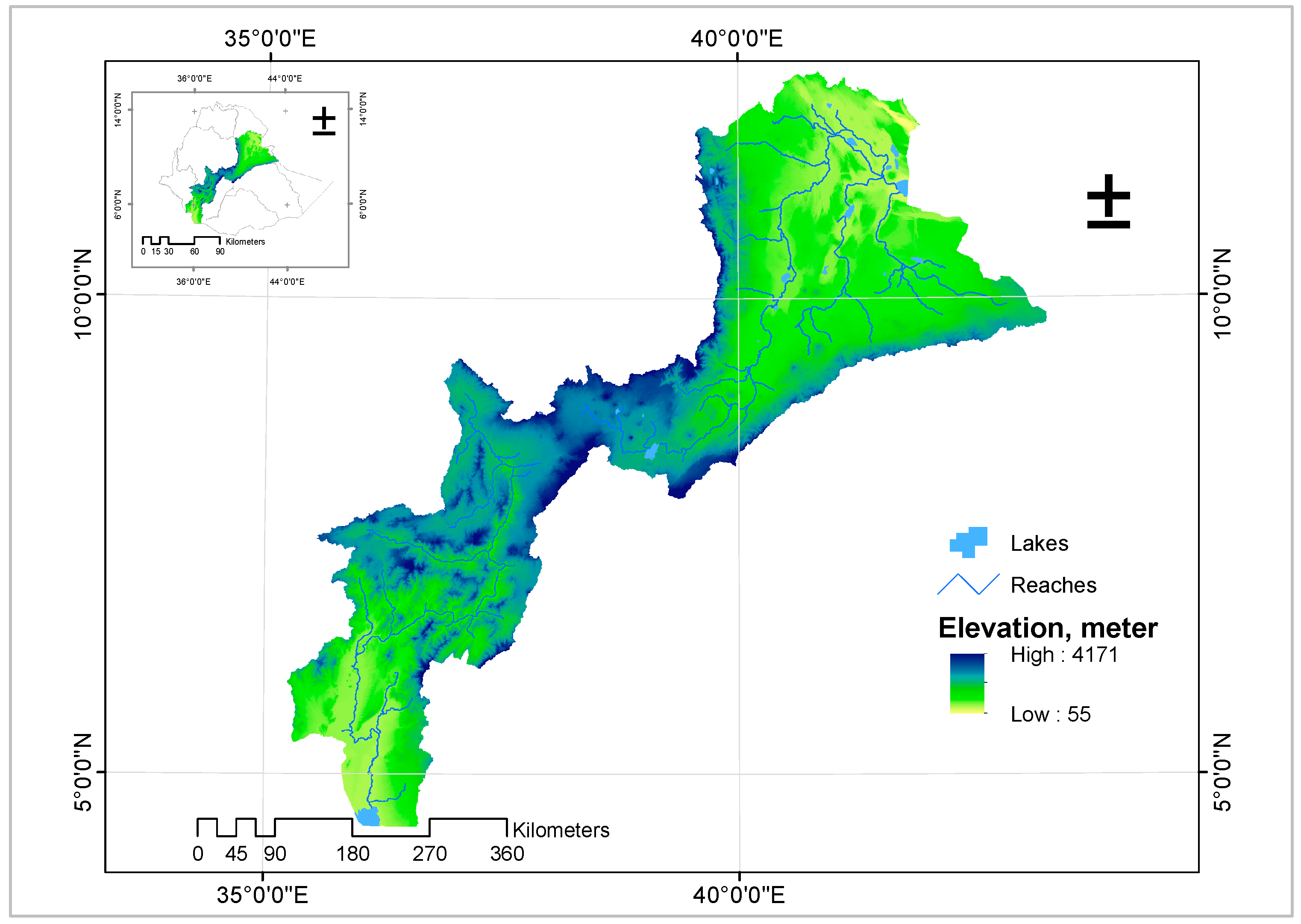
Figure 1. Study area location and surface features.
Remotesensing 14 04518 g001
Figure 2. Annual maximum flow records of Awash-Hombole River.
Remotesensing 14 04518 g002
Figure 3. Processed HMS basin model for simulation.
Remotesensing 14 04518 g003
Figure 4. Observed vs. bias-corrected rainfall for selected weather stations.
Remotesensing 14 04518 g004
Figure 5. Observed vs. predicted runoff for selected rivers in Awash (ad) and Omo-Gibe (e,f).
Remotesensing 14 04518 g005
Figure 6. Observed vs. predicted runoff for selected rivers in Awash and Omo-Gibe basins.
Remotesensing 14 04518 g006
Figure 7. Satellite observation from DFO (left) and model inundation maps (right) in 2006 excluding lake areas, where (a) presents the flood inundation maps in upper Awash (on 3 September 2006); (b) presents the flood inundation maps in middle Awash (on 3 September 2006); (c) presents the flood inundation maps in lower Awash basin (on 3 September 2006); (d) presents the flood inundation map in lower Omo delta (on 21 August 2006).
Remotesensing 14 04518 g007aRemotesensing 14 04518 g007b
Figure 8. Bias-corrected mean daily rainfall for the JJAS 2021 flood season over the basin.
Remotesensing 14 04518 g008
Figure 9. Spatial precipitation distribution for the 2021 flood season (June to September). (a) presents the precipitation distribution for the month of June; (b) presents the precipitation distribution for July; (c) presents the precipitation distribution for August; (d) presents the precipitation distribution for September.
Remotesensing 14 04518 g009
Figure 10. Mean monthly rainfall forecast for the 2021 flood season and historical records.
Remotesensing 14 04518 g010
Figure 11. Seasonal water level forecast for Koka (a) and Gibe-3 (b) reservoirs.
Remotesensing 14 04518 g011aRemotesensing 14 04518 g011b
Table 1. Flood inundations in the model basins based on model and satellite observations.
SNBasin NameRiver NameR2NSEPbiasKGE
1AwashAwash-Kuntire0.730.6843.32−0.142
2Awash-Hombole0.790.71113.84−0.574
3Awash-Below Koka0.820.4552.93−0.137
4Methara0.54-108.36−0.378
5Awash-70.660.5973.74−0.179
6Awash-Sedi0.66-63.91−0.576
7Kesem0.820.3469.42−0.229
8Awash-Werer0.73-31.85−0.095
9Awash-Adaitu0.650.524.41−0.008
10Omo-GibeGibe-Tolai0.780.6022.32−0.048
11Gibe-Abelti0.700.5357.54−0.206
12Gojeb0.44-103.71−0.477
Table 2. Flood inundations in the model basins based on model and satellite observations.
Basin
Name
Floodplain AreaBoundary Conditions (BC)Flood Inundation Area, km2Model Performance
Upstream BC (Energy Slope)Downstream BCCaptured onSatelliteModel
AwashUpper Awash (Hombole to Awash-7)Hydrographs (Hombole, Mojo, and Kelta rivers)Friction slope3 September 2006138.95133.420.96016
Middle Awash (Awash-7 to Gewane)Hydrographs (Awash-7, Arba Bordede and Kesem rivers)522.98454.360.86879
Lower Awash (Gewane to Outlet)Hydrographs (Awash at Adaitu, Mile and Logia rivers)793.93711.620.89632
Omo-GibeLower Omo (Omorate to Outlet)Hydrograph of Omo at OmorateFriction slope21 August 2006241.17187.790.77867
Total1697.031487.18
Table 3. Comparison of observation and forecasted flows and water levels for the 2008 analogue year.
Res. NameYearMonths/SeasonFlows (m3s−1)Reservoir Water Level (m)
Forecasted 2021Observed 2008Forecasted 2021Observed 2008
Koka2008 analogue yearJune41.5055.0104.40102.95
July244.47417.2105.60105.36
August729.44853.3110.00109.70
September276.63515.4111.00110.21
Efficiency of the model results compared between the 2008 analogue year observation and 2021 forecast and reservoir flows and water levels
R20.92230.9916
NSE0.87120.9509
Note: Gibe-3 reservoir is not presented in Table 3 since the reservoir did not exist in 2008.
Table 4. Verification analysis of observed and forecasted flows and water levels for 2021.
Res. NameYearMonths/SeasonFlows (m3s−1)Reservoir Water Level (m)
Forecasted 2021Observed 2021Forecasted 2021Observed 2021
Koka2021 flood seasonJune41.50103.6104.40103.41
July244.47437.1105.60105.85
August729.44891.0110.00108.67
September276.63463.0111.00110.36
Efficiency of the model results between the observed and model flow forecasts and reservoir water levels
R20.97240.9569
NSE0.89790.8861
Gibe-3June128.07336.3858.10862.14
July2482.79942.4869.15871.12
August3658.841529.2888.00885.16
September1984.781058.0892.00891.39
Efficiency of the model results between the observed and model flow forecasts and reservoir water levels
R20.92670.9918
NSE0.91660.9458
Table 5. Reservoir storage and water level forecast based on 2008, the average year, and forecasts.
YearMonthLevelt−1, mArea, km2Volt−1, MCMInflow, MCMRainfall, mmAvg. AreaEvap., mmOutflow, MCMSeepage, MCMVolt, MCMR. Levelt, m
Koka Reservoir
2008June104.67125.77294.3450.9293.10122.09200.00119.912.44209.86103.90
July103.90118.40209.86387.61251.90128.80184.00110.292.37493.56106.20
August106.20139.20493.56786.49251.90153.39174.00244.702.671044.63109.50
September109.50167.571044.63481.53133.70167.57174.00256.662.921259.83110.58
Average yearJune104.67125.77294.3492.5058.00124.29200.00119.912.49246.79104.20
July104.20122.80246.79397.2283.00131.20184.00110.292.41518.06106.40
August106.40139.60518.06813.95212.00155.94174.00244.702.711090.53109.80
September109.80172.291090.53424.68186.00172.29174.00256.663.001257.62110.62
ForecastedJune104.67125.77294.340.3557.49123.74200.00119.912.47154.67103.30
July103.30121.70154.67375.65201.17133.95184.00110.292.46419.87105.70
August105.70146.20419.87891.01172.55161.60174.00244.702.811063.14109.60
September109.60177.001063.1474.8690.01177.00174.00256.663.081263.39110.60
Gibe-3 Reservoir
2008June865.71157.5010,056.501105.6 204.00158.7569.001040.671.1010,141.76866.00
July866.00160.0010,141.763253.0 241.00167.5056.40988.800.9412,435.94880.00
August880.00175.0012,435.945784.2 236.00187.5059.601115.971.1217,136.12894.00
September894.00200.0017,136.123416.1 163.00200.0067.601944.371.3518,625.58894.00
Average yearJune865.71157.5010,056.50897.00204.00157.5069.001040.671.099933.00864.00
July864.00157.509933.002542.90241.00162.5056.40988.800.9211,516.18874.00
August874.00167.5011,516.184078.90236.00176.2559.601115.971.0514,509.15894.00
September894.00185.0014,509.152739.40163.00185.0067.601944.371.2515,320.58894.00
ForecastedJune865.71157.5010,056.50219.5457.49158.7569.001040.671.109232.45860.10
July860.10160.009232.452278.89201.17168.7556.40988.800.9510,546.01869.15
August869.15177.5010,546.014179.83172.55188.7559.601115.971.1213,630.06890.00
September890.00200.0013,630.102024.5190.01200.0067.601944.371.3513,713.33892.00
Publisher’s Note: MDPI stays neutral with regard to jurisdictional claims in published maps and institutional affiliations.