Underwater Object Detection Based on Improved EfficientDet

Abstract

Intelligent detection of marine organism plays an important part in the marine economy, and it is significant to detect marine organisms quickly and accurately in a complex marine environment for the intelligence of marine equipment. The existing object detection models do not work well underwater. This paper improves the structure of EfficientDet detector and proposes the EfficientDet-Revised (EDR), which is a new marine organism object detection model. Specifically, the MBConvBlock is reconstructed by adding the Channel Shuffle module to enable the exchange of information between the channels of the feature layer. The fully connected layer of the attention module is removed and convolution is used to cut down the amount of network parameters. The Enhanced Feature Extraction module is constructed for multi-scale feature fusion to enhance the feature extraction ability of the network to different objects. The results of experiments demonstrate that the mean average precision (mAP) of the proposed method reaches 91.67% and 92.81% on the URPC dataset and the Kaggle dataset, respectively, which is better than other object detection models. At the same time, the processing speed reaches 37.5 frame per second (FPS) on the URPC dataset, which can meet the real-time requirements. It can provide a useful reference for underwater robots to perform tasks such as intelligent grasping.

1. Introduction

Marine object detection is one of the important fields of marine technology research [1,2,3]. In the past, underwater object detection relied on divers, but the long-term underwater operations and complex underwater environment place a serious impact on their bodies. Underwater robots can help humans in underwater operations, which have the ability to identify and locate objects quickly and accurately [4,5,6,7]. Therefore, real-time detection of underwater object has a great research value and considerable application prospects. The objective of this paper is to study the object detection algorithm based on marine organisms, which can provide technical support for the monitoring, protection and sustainable development of marine fish and other biological resources.

The existing object detection methods fall into traditional methods and deep learning-based methods. The traditional methods generally fall into three relatively independent parts: region selection, feature extraction and classification by classifier. The accuracy and speed of its detection are not ideal.

As the artificial intelligence develops continuously, deep learning is widely used in speech recognition, natural speech processing, signal modulation and recognition, image analysis, optical communication and other fields [8,9,10,11,12]. Object detection algorithms grounded on deep learning have become a new research focus. Convolutional neural network (CNN) is the main method of deep learning applications, which improves the quality of learning by increasing the amounts of convolutional layers. CNN uses the backpropagation algorithm for feedback learning, which minimizes human intervention and improves learning ability by automating feature extraction and multi-layer convolutional learning [13]. Therefore, compared with the traditional detection methods with manual feature extraction, the learning effect of deep learning-based detection methods is better.

Object detection algorithms grounded on deep learning are roughly classified into two kinds: one is the two-stage algorithms based on classification, for example, R-CNN, Fast R-CNN, and Faster R-CNN [14,15,16]; the other one is the one-stage algorithms based on regression, for example, YOLO [17] and SSD [18]. Many researchers have also applied these deep learning algorithms to underwater object detection. Lingcai Zeng added the adversarial network to the Faster R-CNN for training [19], which improved the detection ability, but can only perform static detection. Yong Liu embedded a convolution kernel adaptive selection unit in the backbone of the Faster R-CNN [20], which further increased the detection accuracy, but its FPS is 6.4, which also fails to satisfy the needs of real-time detection. YOLO is characterized by fast detection speed and it has good detection ability in the environment with clear field of view and obvious object characteristics, but it is not effective when used in underwater environment. Yan Li improved the in situ detection performance of plankton by embedding DenseNet in YOLOv3 [21]. The backbone network structure of SSD is deep and has more parameters. It is not conducive to deployment on hardware and the ability to detect small objects is poor. Jun Yue improved SSD by the MobileNet to obtain higher detection accuracy [22]. Kai Hu used feature enhancement approach to highlight the learning of detailed characteristics of echinus. And ResNet50 is used instead of VGG16 to expand the field of view for object detection. However, the complex network structure has not improved yet [23]. Ellen M. Ditria from Australia uses Mask R-CNN to detect fish abundances inhabiting the east coast of Australia and achieves better results than Human Marine Experts. It is advantageous for monitoring fish biodiversity in their natural habitats [24]. To overcome the challenges present in underwater videos due to a range of factors, Ahsan Jalal propose a hybrid solution to combine optical flow and Gaussian mixture models with YOLO deep neural network, which achieves the best fish detection results in a dataset collected by The University of Western Australia (UWA) [25]. Two researchers from the UK have also conducted related research. Sophie Armitage from University of Exeter uses the YOLOv5 framework to detect underwater plastic litter in the southwest of England and achieves a very high accuracy of 95.23%. However, for images with accumulations of multiple plastics, the model often failed to identify some objects and misidentified others due to YOLO operates in a single pass over the image, reducing the capacity of the model to detect multiple small objects in close proximity [26]. Ranjith Dinakaran from Northumbria University proposes a cascaded framework by combining the deep convolutional generative adversarial network (DCGAN) with SSD, named DCGAN + SSD, for the detection of various underwater objects. Though the detection accuracy of the model is higher than the original SSD, it is not fast enough to achieve real-time detection on automated underwater vehicles (AUVs) [27]. Therefore, how to balance the speed and accuracy of detection to improve the efficiency of object detection is still a challenge that needs to be tackled for marine organism object detection.

The object detection framework called EfficientDet was invented in 2020 [28], and the authors innovatively proposed compound scaling and Bidirectional Feature Pyramid Network (BiFPN), a feature fusion network that adds contextual information weights to the original feature pyramid network and performs top-down and bottom-up fusion. The excellent network structure balances the speed and accuracy of detection well. However, the Depthwise convolution (DWConv) in MBConvBlock will split the information between different channels, which is not conducive to information exchange between different channels. The ability of a single feature pyramid network to extract the characteristics of the object in depth still needs to be improved due to the complex environment of the seafloor, uneven distribution of brightness, poor differentiation between marine organisms and their living environment and organisms being obscured or semi-obscured and so on.

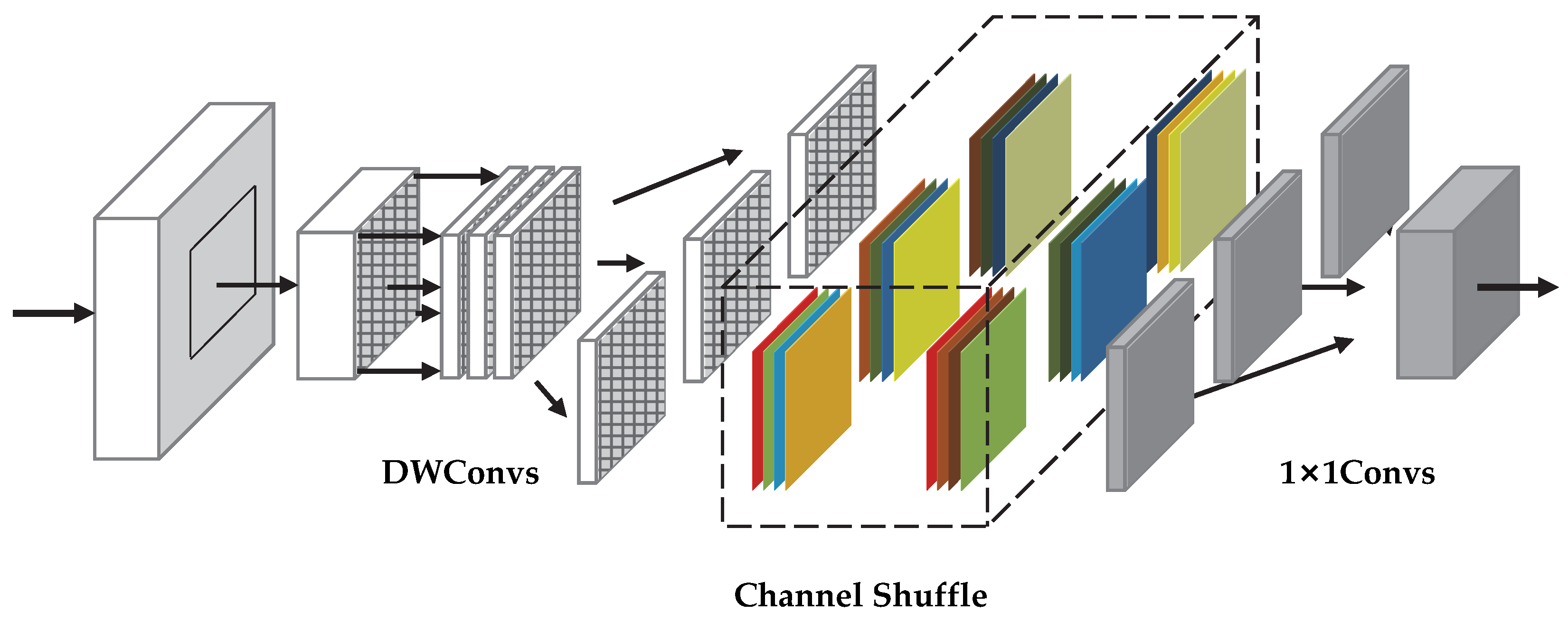
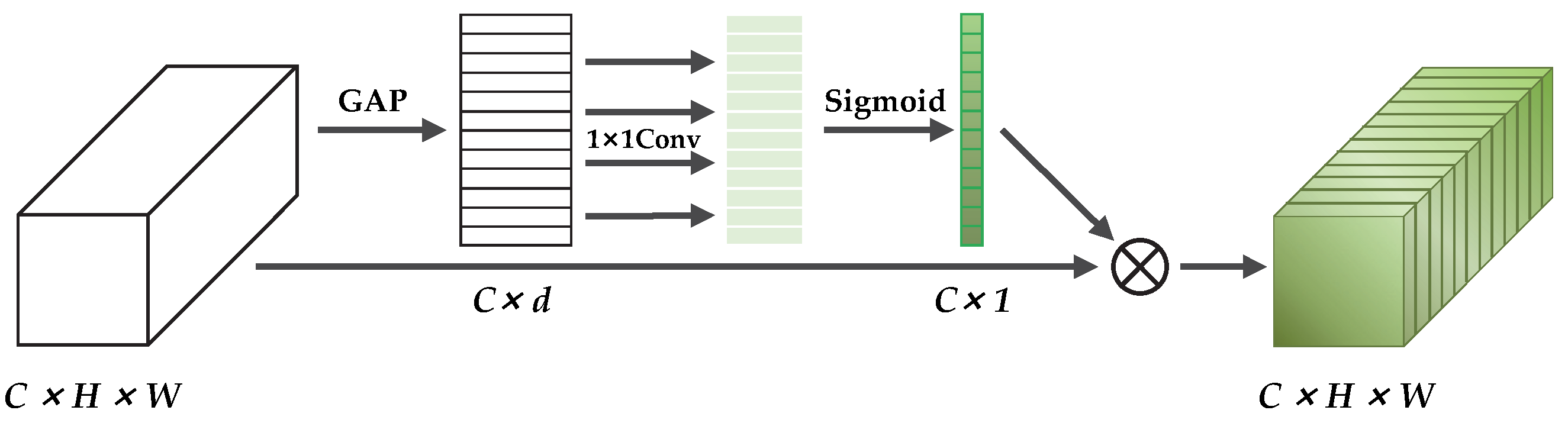
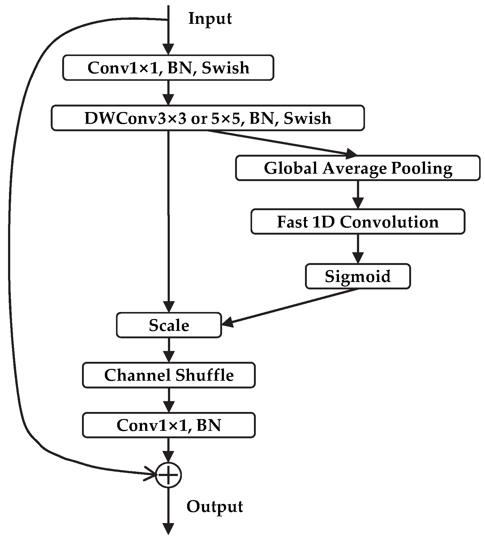
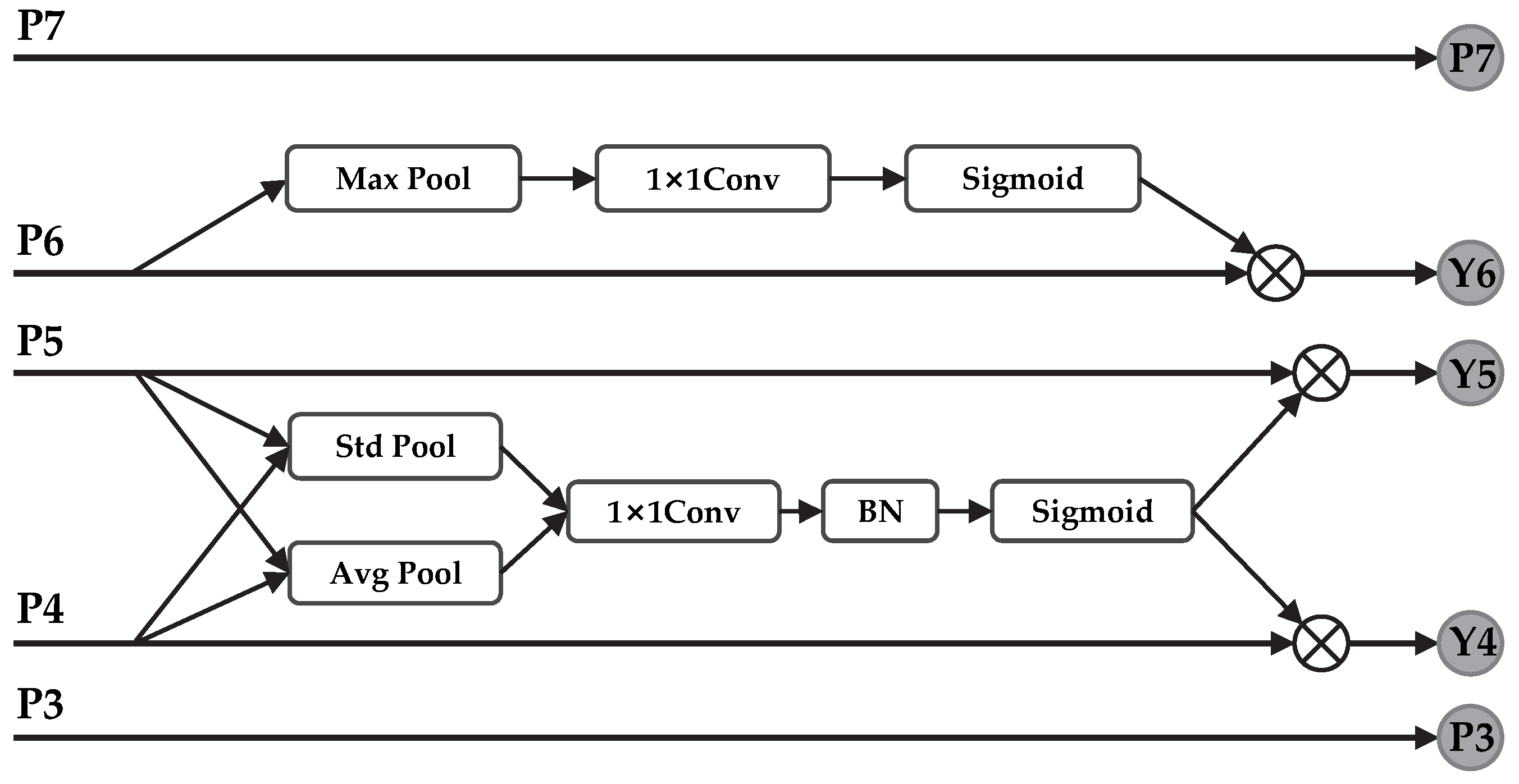
To address these shortcomings, a marine organism object detection model is proposed in this paper, which is called EfficientDet-Revised (EDR). It is based on the improved EfficientDet network. The chief achievements are as follows: (1) the Block of the model is improved by adding the channel shuffle module [29] after the DWConv (3 × 3 or 5 × 5), which makes information between the channels in the feature layer can be fused to enhance the feature extraction capability of the network. (2) Removing the fully connected layer of the attention module in Block and using 1D convolution for learning can effectively capture cross-channel interactions, and cut down the complexity of the network to improve the detection efficiency. (3) In view of the complex characteristics of underwater objects and the shortcomings of EfficientNet in this aspect, this paper constructs Enhanced Feature Extraction module for multi-scale feature fusion after layers P4, P5, and P6 (corresponding to low-layer, middle-layer, and high-level feature maps, respectively). It adopts the thought of feature cross-layer fusion to complete the connection of different network layers, which enhances the contextual information. In the meantime, it improves the capability of the CNN to express the objects with different scales and strengthen the semantic information.

The contents of this paper are as follows: Section 2 presents EefficientDet; Section 3 introduces the improved network algorithm in detail; Section 4 describes the experimental process, and gives and discusses the experimental results; and Section 5 gives a summary of the full text.

2. EfficientDet

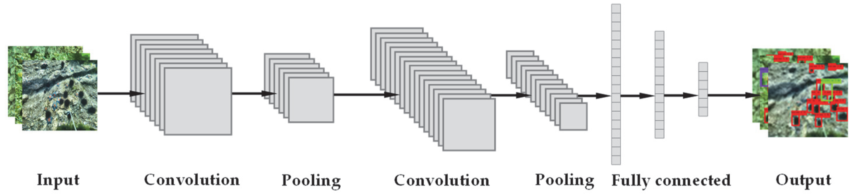
The CNN contains convolutional computation and have a deep structure. It includes convolutional layers, pooling layers and fully connected layers. The connections between the convolutional layers are called sparse connection which is used to reduce the connections between the network layers and the amounts of parameters and make the operation easy and efficient. The nature of weight sharing in CNN improves the stability and generalization ability of the network structure, avoids overfitting and enhances the learning effect [30,31]. The structure of model is shown in Figure 1.

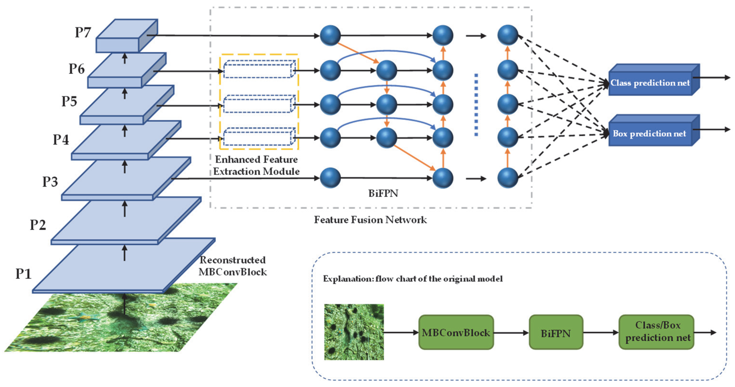
EfficientDet is one of the most advanced object detection algorithms, which has a simple structure and excellent performance. It is available in seven versions from D0 to D6. And the resolution, depth and width of the model can be scaled simultaneously by it according to resource constraints to meet the detection requirements under different conditions. By using the EfficientNet as the backbone network, BiFPN as the feature network, and the shared class/box prediction network, EfficientDet balances the speed and accuracy in the object detection task well.

2.1. Backbone Network

Enhancing the depth of the neural network, adding the width of the feature layer, and increasing the resolution of the input image can improve the detection accuracy of the network [32,33,34], but also lead to more network parameters and higher computational costs.

To improve the detection efficiency, balancing the dimensions of network width, depth and resolution is crucial during CNN scaling. EfficientNet combines these three characteristics and puts forward a new model scaling method that uses an efficient composite coefficient to simultaneously adjust the depth, width, and resolution of the network. Grounded on the neural structure search technology [35], the optimal composite coefficient can be obtained. As shown in equations.

$$depth:d={\alpha }^{\varphi }$$

(1)

$$width:w={\beta }^{\varphi }$$

(2)

$$resolution:r={𝛾}^{𝜙}$$

(3)

$$\alpha \cdot {\beta }^2\cdot {\gamma }^2\approx 2$$

(4)

where $\left(\alpha , \beta , \gamma \right)$ represent the weight of depth, width and resolution, respectively, and are constants that can be determined by small network search, and $\varphi$ is a user-specified factor that controls the number of resources used for model scaling.

Under this constraint, $\alpha =1.2$, $\beta =1.1$ and $\gamma =1.15$ are obtained. When $\varphi =0$, an optimal base model EfficientNet-B0 is obtained; when the $\varphi$ is increased, it is equivalent to expanding the three dimensions of the base model at the same time, and the model becomes larger, the performance also improves, and the resource consumption also becomes larger.

The structure of EfficientNet is shown in Figure 2.

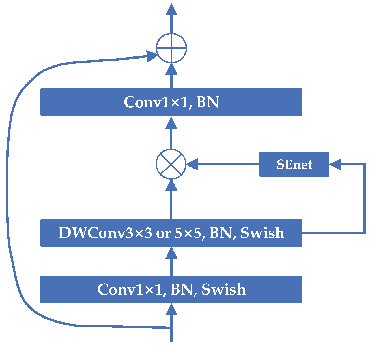
The general structure of Block is shown in Figure 3, and its design idea is Inverted Residuals, using 1 × 1 convolution to up-dimension before the 3 × 3 or 5 × 5 DWConv, adding a channel attention mechanism after the DWConv, and finally adding a large residual edge after using 1 × 1 convolution to down-dimension. BN is the BatchNorm.

2.2. BIFPN

The top feature map has rich semantic information but low resolution, while the bottom feature map has low-level semantic information but higher resolution. Multi-scale feature fusion is the aggregation of features with different resolution semantic information, so that the network has the ability to detect features of different scales.

FPN, NAS-FPN, PANet, etc., [36,37,38] have been widely used in multi-scale feature fusion. However, their direct combinations of the feature maps in different layers and ignores the contribution of different resolution features to the output features. The authors proposed BiFPN, which is simple and efficient. As shown in the formula, the importance of different input features to feature fusion is expressed by calculating the weights of different layers.

$$O={\displaystyle \sum }_i\frac{w_i}{ϵ+{{\displaystyle \sum }}_j{w}_j}\cdot I_i$$

(5)

where $w_i$ is the learnable weight, which can be a scalar, a vector, or a multidimensional tensor. The output weight can be controlled to be in the 0–1 by Relu and simple regularization.

3. Methods

EfficientDet is an efficient object detection framework. Usually, the computing resources and memory of the underwater platform are limited, the underwater environment is complex, and the characteristics of objects are not obvious. All these create obstacles for EfficientDet to be applied in practice. Therefore, it is necessary to improve the extraction capability of underwater object characteristics with limited resources and enhance the efficiency of object detection.

To handle this problem, the structure of EfficientDet is improved and a detector which is more effective for underwater applications is designed in this paper. Based on EfficientDet, the MBConvBlock in the backbone network is improved and an Enhanced Feature Extraction network is designed for multi-scale feature fusion before BiFPN. The improved object detection algorithm, called EDR, is a more comprehensively efficient object detection framework. The overall structure is shown in Figure 4.

3.1. Feature Extraction Network

In underwater object detection scenarios, the research of neural networks tends to be applied on mobile devices. In order to ensure the deep neural networks can be better deployed on underwater robots, in the meantime, to provide realistic feasibility for model expansion in different scenarios and under different conditions, the MBConvBlock is reconstructed in this paper by using Channel Shuffle. The reconstructed MBConvBlock is shown in Figure 5.

In this paper, Channel Shuffle is first added after DWConv to help information flow among feature channels. Unlike conventional convolution where each convolution kernel operates on each channel of the input image simultaneously, one convolution kernel of DWConv is responsible for only one channel. The number of parameters and the cost of this operation are low, but it operates each channel of the input layer independently and does not use the feature information of different channels effectively in the same spatial position. Therefore, it is not conducive to the flow of information among the feature channels. In order to make effective communication of the information among the feature maps of different channels, Channel Shuffle is used to reorganize the feature maps of different channels. By this way, it can make the input of DWConv in the next MBConvBlock come from different feature channels, then more effective feature information can be obtained. The procedure for Channel Shuffle is as follows. Suppose the number of convolutional layers after DWConv is ‘a’ and the number of channels in each convolutional layer is ‘b’. The output has a x b channels. The first step is Reshape: the dimension of the input channel is reshaped into (a, b). The next step is Transpose: (a, b) is transposed to (b, a). The final step is Flatten: flattening (b, a) back as the input of next layer. Figure 6 shows the workflow of Channel Shuffle.

Secondly, the attention module of MBCconvBlock has two fully connected layers, which have a large amount of parameter redundancy and it is difficult to analyze the correlation of channels between different layers. In contrast, convolution has good cross-channel information acquisition ability and replacing the fully connected layer can effectively reduce the amounts of parameters of the network. To handle the above problems, a new feature attention module is constructed. The structure is shown in Figure 7. For the feature layer entered, the Global Average Pooling (GAP) is implemented to obtain the global spatial information. Then, the cross-channel information integration is achieved by 1 × 1 convolution to enhance the spatial correlation of the features. After that, Sigmoid is taken to obtain the weight (0–1) for each feature point of the input feature layer. After obtaining this weight, we just multiply this weight by the original input feature layer. GAP is often used to aggregate spatial information, as shown in the following formula.

$$A_c=\frac{1}{H\times W}{{\displaystyle \sum }}_{a=1}^H{{\displaystyle \sum }}_{b=1}^W{X}_c\left(a,b\right)$$

(6)

where $A_c$ is the value of feature map after GAP, $X_c\left(a,b\right)$ is the value of the input channel, and $H$ and $W$ are the width and height of the input feature map.

The weights of feature maps of different channels can be obtained by the following operations.

$$U_c=\sigma \left(W\ast A_c\right)$$

(7)

where $W$ is the weight matrix of the 1 × 1 convolution, and $\sigma$ is the Sigmoid function.

Finally, the feature channels are recalibrated. The equation is as follows.

$$Y_c=U_c\otimes X_c$$

(8)

where $Y_c$ is the value of output channel after recalibration.

3.2. Multi-Scale Feature Fusion Network

How to effectively handle multi-scale features is one of the difficulties of object detection. Given the complexity of the underwater environment, underwater images are usually characterized by color shift and low contrast. In addition, the diverse sizes and inconspicuous characteristics of the underwater objects make it difficult to detect underwater objects. At the same time, due to the living habits of marine organisms, they are usually close to each other in the images. Combined with these realities, this paper designs an Enhanced Feature Extraction module to form a multi-scale feature fusion network to improve the representation ability of CNN on objects of different scale features before BiFPN. The structure of the Enhanced Feature Extraction Module is shown in Figure 8.

First, the middle feature layers, P4, P5 and P6, of the backbone feature network (corresponding to the lower, intermediate, and higher feature maps, respectively) are used as inputs, and the global information of the features is obtained by using Avgpool and Stdpool for the P4 and P5 layers, and Maxpool for P6 layer. Then, the interdependencies between channels are obtained through 1 × 1 convolution layers. After that, it is normalized by BN (the P6 layer does not it), and Sigmoid is taken to get the channel weights (0–1). Finally, the weights are multiplied by P4, P5 and P6 layers, respectively, as new feature layers and input to the BiFPN, while the feature fusion from top-down and bottom-up is iteratively performed. The top feature map has rich semantic information, Maxpool can well retain detail characteristics, such as texture, while the bottom feature map has high resolution, the background information can be well preserved with Avgpool and Stdpool. The specific formulas are as follows.

$${\mu }_c=\frac{1}{HW}{\displaystyle \sum }_{i=1}^H{\displaystyle \sum }_{j=1}^W{X}_{i,j}$$

(9)

$${\xi }_c=\sqrt{\frac{1}{HW}{\displaystyle \sum }_{i=1}^H{\displaystyle \sum }_{j=1}^W{\left(X_{i,j}-{\mu }_c\right)}^2}$$

(10)

$$g\left(x\right)=\left[{\mu }_c,{\xi }_c\right]$$

(11)

where $X_{i,j}$ is the value of the input channel, ${\mu }_c$ is the feature vector after Avgpool, ${\xi }_c$ is the vector representation after Stdpool of the feature layer, and $g\left(x\right)$ is the feature information after the splicing of Avgpool and Stdpool.

After obtaining the pooling information of the feature map, the following operation is performed to obtain the weights of the feature map for each channel.

$$S=\sigma \left(BN\left(C1D\left(g\left(x\right)\right)\right)\right)$$

(12)

where $\sigma$ denotes the Sigmoid function and BN is to normalize. $C1D$ indicates 1D convolution and it is used to obtain the correlation between channels. S represents the weight of channel-wise.

Finally, the original input is recalibrated by the weight. Thus, the output of the P4 and P5 layers are as follow.

$$Y_{4,5}=SX$$

(13)

The P6 layer uses Maxpool. The formulas are as follows.

$$M_c=\underset{i=1,j=1}{\overset{p}{\mathit{max}}}\left(X_{ij}\right)+b$$

(14)

$$S=\sigma \left(C1D\left(M_c\right)\right)$$

(15)

$M_c$ is the feature vector after Maxpool, then the output of the P6 layer is as follows.

$$Y_6=SX$$

(16)

4. Experiments

This experiment aims to illustrate the effectiveness of EDR algorithm in marine organism object detection. All experiments are conducted on Linux system. The GPU version required for the experiment is NVIDIA GTX 1080 (16G RAM). The software environments are Pytorch 1.2.0 on Python 3.6, Anaconda 3, CUDA 10.0 and CUDNN 7.3.0. The training epochs are set to 200. The batch size is set to 16 based on the performance of the graphics card. The learning rate is initially 0.01 and then is reduced by 10 times when epoch is 100 and 150.

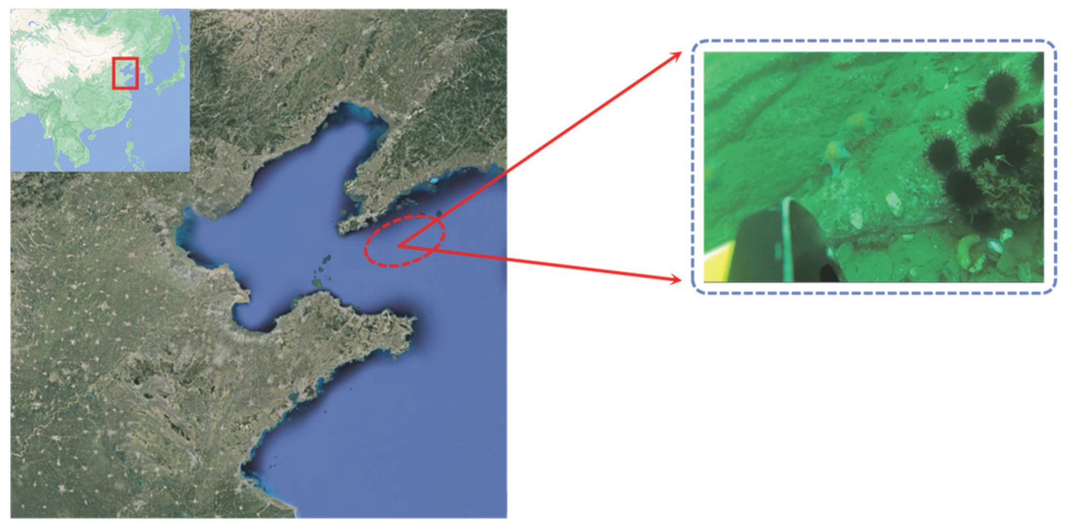
The dataset is supplied by the National Natural Science Foundation for Underwater Robotics Professional Competition (URPC). It is labeled by labelImg, and the image format is PASCAL VOC, which includes four species: echinus, holothurian, scallop, and starfish. As shown in Figure 9, these data are collected by Remotely Operated Vehicle (ROV) in the sea off Dalian City, Liaoning Province, China, and are common marine organisms near the coast of China. There are 5543 images in the dataset, fall into training sets, validation sets, and test sets in the ratio of 7:2:1.

Figure 10 shows the proportional distribution of the size of each object to the size of the image. From the figure, it can be seen that the size proportion distribution of objects is relatively scattered, but most of them are concentrated in 0.1 to 0.3, which requires the model to have a good ability of multi-scale feature fusion.

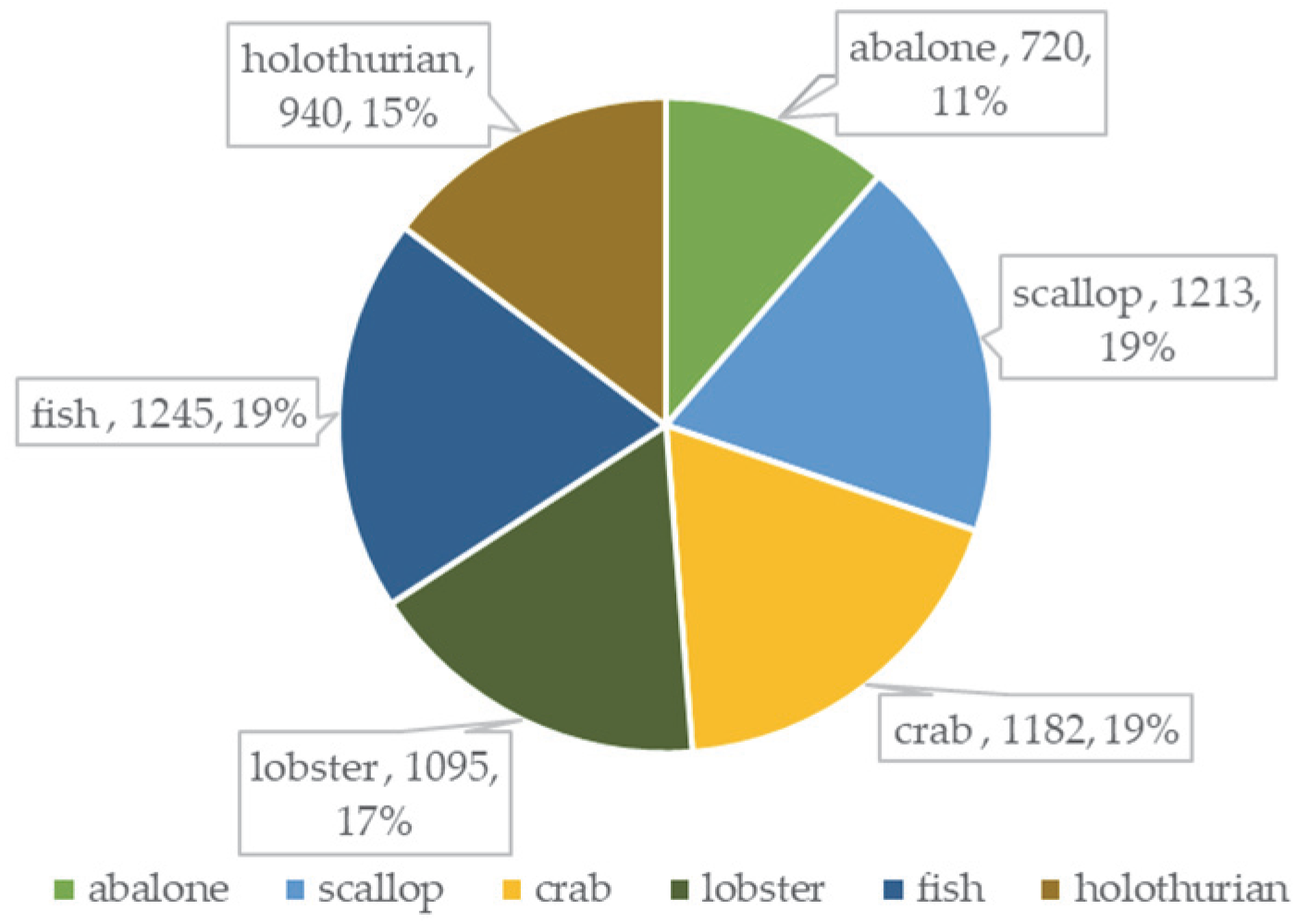
In order to verify the robustness of the model, some images of marine organisms are collected at Kaggle and make into a dataset in the same format. The dataset includes six species: abalone, crab, fish, holothurian, lobster and scallop. There are 6396 images in total. Figure 11 shows the number of each species in this dataset, and the distribution of category samples in this dataset is relatively balanced.

4.1. Evaluation Indicators

The Intersect Over Union (IOU) threshold parameter needs to be set for the model prediction. When the IOU > 0.5, the detection is successful. In this paper, the mean Average Precision (mAP), Frames Per Second (FPS), and model size are used as evaluation indicators. First, it introduces Precision and Recall. The Precision is the ratio of correctly predicted positive classes to all predicted positive classes, and the Recall is the ratio of correctly predicted positive classes to all actual positive classes. The formulas are shown as follows.

$$Precision=\frac{TP}{TP+FP}$$

(17)

$$Recall=\frac{TP}{TP+FN}$$

(18)

where $TP$ is the number of positive classes that are correctly predicted, $FP$ is the number of negative classes that are predicted as positive classes, and $FN$ is the number of positive classes that are predicted as negative classes. To measure the true level of detection, the value of AP was used to represent it as follows.

$$AP={{\displaystyle \int }}_0^{1}P\left(R\right)dR$$

(19)

mAP is the mean of the AP values of all categories, and the larger the mAP is, the higher the object detection accuracy of the algorithm has. The formula for mAP is as follows.

$$mAP=\frac{1}{n}{\displaystyle \sum }_{i=1}^n{{\displaystyle \int }}_0^{1}P\left(R\right)dR$$

(20)

where $n$ represents the number of categories detected.

Frames Per Second (FPS) indicates the number of images the algorithm can process per second, which is used to assess the detection speed of the algorithm. The minimum fluency of human eye recognition can be met when the frame rate >24 fps.

4.2. Results and Analysis of Experiments

First, the preliminary experiments with EfficientDet are conducted on the URPC public dataset. The versions of D0, D1 and D2 are trained due to resource limitation. The results are shown in

Table 1. The experimental results for different versions of EfficientDet.

Methods	Backbone	Storage Size (/MB)	mAP (%)	FPS
EfficientDet-D0	EfficientNet-B0	14.9	84.67	45.1
EfficientDet-D1	EfficientNet-B1	25.5	87.71	40.3
EfficientDet-D2	EfficientNet-B2	31.1	89.37	38.8

. As the compound scaling deepens, the mAP gets higher. At the same time, the size of the model is increasing and the FPS is getting smaller.

Even though EfficientDet-D2 has the highest accuracy, it consumes a lot of computational resources and is comparatively not easy to train. EfficientDet-D0, as the lightest model, is smaller and faster. EfficientDet-D0 is selected as the baseline and ablation experiments are conducted to verify the impact of different improvements on model performance.

Table 2. The results of ablation experiments.

Model	Method				Storage Size (/MB)	mAP (%)	FPS
	Baseline	CS	EFEM	1D Convolution
EfficientDet-D0	√				14.9	84.67	45.1
*	√	√			16.2 (+8%)	85.23 (+0.56)	39.5
**	√	√	√		21.5 (+32%)	86.83 (+1.6)	28.3
EDR-D0	√	√	√	√	15.7 (−26%)	86.83 (+0)	43.9

shows the results of the ablation studies performed on D0. ‘*’is the model that adds Channel Shuffle (CS) to the backbone. ‘**’is the model in which the Enhanced Feature Extraction module (EFEM) is added to ‘*’.

The results indicate that the model size and mAP of model ‘*’ increase by 8% and 0.56% respectively, while the FPS decrease by 4.6 compared with the original model. The addition of Channel Shuffle has resulted in some improvement in the accuracy of the model. The construction of the Enhanced Feature Extraction module result in a further 32% and 1.6% increase in model size and mAP for model ‘**’, respectively, while the FPS is only 28.3. As can be seen, the Enhanced Feature Extraction module contributes significantly to the accuracy improvement, but also leads to a large drop in the performance of other metrics. After replacing the fully connected layer with 1D convolution, the model size and FPS of the EDR are somewhat improved.

The further experiments are carried out on the URPC public dataset to compare the model proposed in this paper with other commonly used object detection models. The results of the experiment are shown in

Table 3. The experimental results with different object detection models.

Method	Backbone	Storage Size (/MB)	mAP (%)	FPS
Faster R-CNN	ResNet50	108	81.88	7.4
Faster R-CNN-FPN	ResNet-50-FPN	133	84.71	5
SSD	VGG16	235	79.25	56.2
Mobile-SSD	MobileNet	46.1	71.67	105
YOLOv4	CSPDarkNet53	91.4	78.61	71
CenterNet	ResNet50	82.6	75.79	60.7
RetinaNet	ResNet50	77	73.75	52.2
EfficientDet-D0	EfficientNet-B0	14.9	84.67	45.1
EfficientDet-D1	EfficientNet-B1	25.5	87.71	40.3
EfficientDet-D2	EfficientNet-B2	31.1	89.37	38.8
EDR-D0	/	15.7	86.83	43.9
EDR-D1	/	26.8	89.90	38.6
EDR-D2	/	33.1	91.67	37.5

.

As can be seen from Table 3, in longitudinal comparison, the highest mAP of the algorithm put forward in this paper reaches 91.67%, which is 2.3% higher than the original detection algorithm. The improvement of mAP is mainly due to the construction of the multi-scale feature fusion network, which makes the model’s ability to grasp the object information enhanced. For underwater study, people focus more on the characteristics of the object to improve the detection capability. In horizontal comparison, it can be seen that the mAP of the EDR algorithm is higher than the other algorithms. Despite its poor performance in terms of speed, the EDR can also meet the requirements of real-time detection. Furthermore, the model size of EDR is much lower than the other methods, which can facilitate its deployment in ROV, so that ROV can have more memory space to expand and enrich the functions. These advantages stem from the good network design of EDR algorithm. The two-stage object detection algorithm represented by Faster R-CNN has good detection accuracy, but its detection speed is only 7.4 frames per second, which cannot meet the real-time requirement. Even though the addition of Feature Pyramid Network increases its detection accuracy by 2.83%, it can only do static detection. YOLOv4 is the representative of one-stage object detection algorithm, which has a good speed performance but poor detection accuracy performance. SSD perform well in both speed and accuracy, but its model size is not conducive to deployment on mobile devices. Mobile-SSD solves this problem very well, but mAP and FPS are greatly reduced. CenterNet and RetinaNet also perform mediocrely on various metrics. In general, in terms of marine organism object detection, EDR achieves a balance between speed and accuracy at a smaller cost.

Figure 12 shows the AP comparison of different models, covering various categories of the dataset. For each category of objects, the detection accuracy of EDR is significantly better compared with the other methods.

To verify the validity of the model, the parallel experiments are conducted on Kaggle dataset.

Table 4. The results of different categories between different models on homemade dataset.

	Category	Abalone (%)	Crab (%)	Fish (%)	Holothurian (%)	Lobster (%)	Scallop (%)	mAP (%)
Methods
Faster R-CNN		73.79	83.77	79.90	83.90	84.67	85.78	81.97
Faster R-CNN-FPN		78.88	82.87	80.78	86.76	89.01	91.85	85.02
SSD		70.32	81.63	83.89	76.02	78.53	85.24	79.27
Mobile-SSD		64.71	71.74	72.67	69.86	70.02	75.32	70.72
YOLOv4		60.96	82.58	79.87	80.80	72.98	83.27	76.74
CenterNet		66.22	74.69	69.31	73.32	78.67	71.96	72.36
RetinaNet		69.22	73.54	74.16	81.82	72.84	76.08	74.61
EfficientDet-D0		81.60	92.19	79.71	78.28	85.71	89.17	84.44
EfficientDet-D1		83.19	91.78	86.05	83.48	90.21	89.09	87.30
EfficientDet-D2		88.49	94.27	89.84	86.16	91.29	95.56	90.94
EDR-D0		83.96	94.41	84.08	79.18	90.55	90.42	87.10
EDR-D1		90.44	94.09	87.56	84.01	93.08	90.63	89.97
EDR-D2		92.81	94.49	90.37	88.04	92.79	95.85	92.39

shows the detailed detection results of each category of object between different models. Bolded text indicates the best result. It is obvious that the method in this paper achieves the highest AP on all kinds of objects, and the mAP reaches a maximum of 92.39%. The experimental results show that the proposed method can meet the detection requirements of different situations.

The visual detection results are shown in Figure 13. Two images are selected at random, the images in the first row contain single-category objects, and the images in the second row contain multi-category objects. From the test results, it can be seen that the method in this paper is more effective than other methods whether objects are single-category or multi-category.

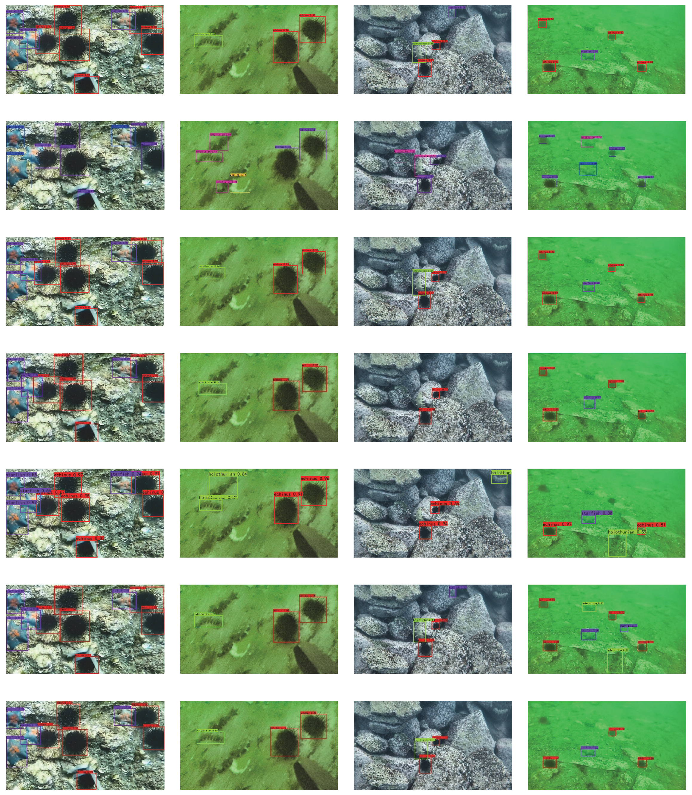
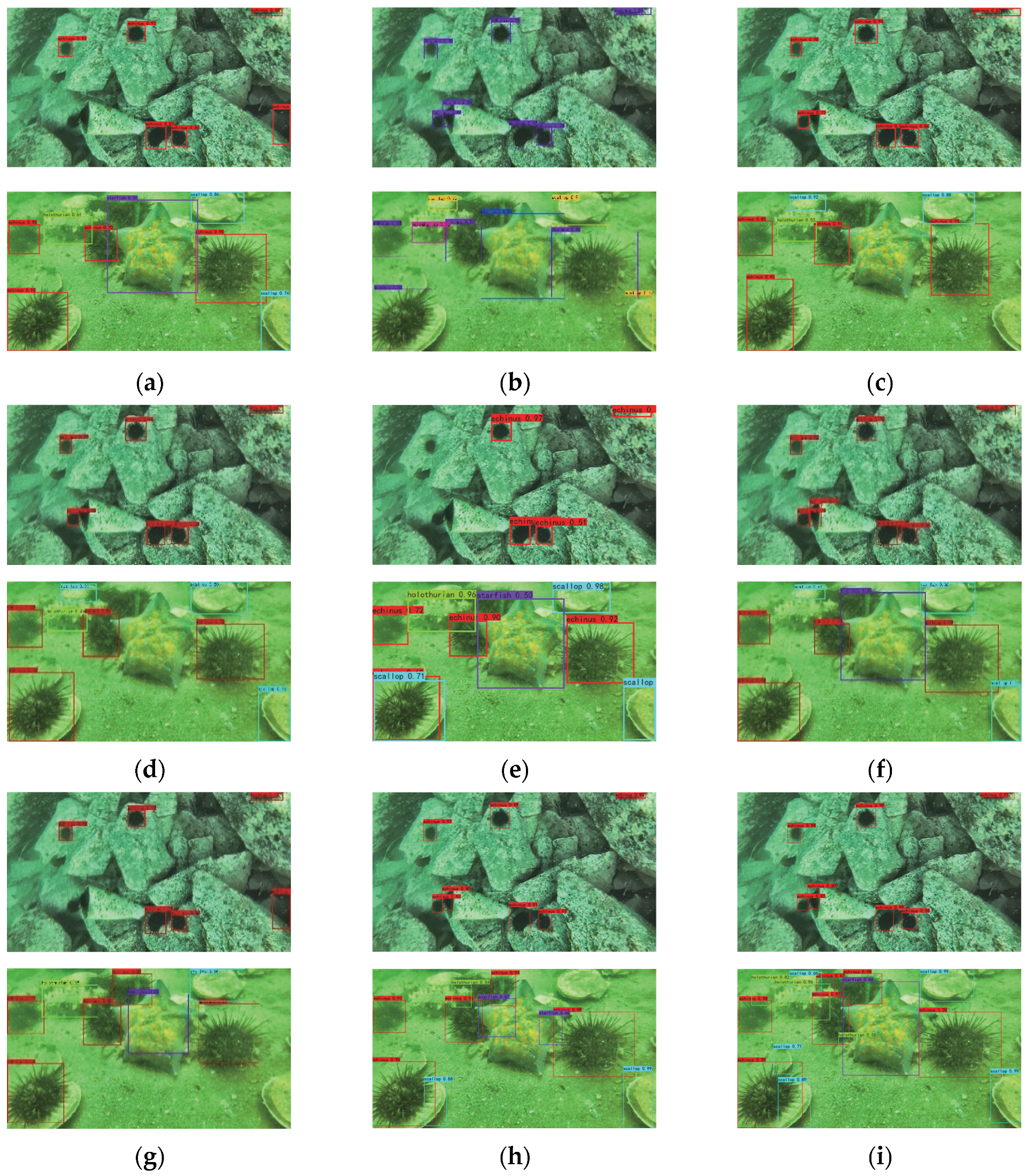
As shown in Figure 14, to understand the detection results more realistically, the experiments are conducted in the four scenes, which are close-range clear, close-range blur, long-range clear, and long-range blur. From the results, it can be seen that each method can accurately detect the object in the close-range clear scenes. However, for the other scenes, all of the other methods have low accuracy and missed detection whether it is a long distance or a blurry image. While the method in this paper has higher accuracy and lower rate of missed detection for objects, and it has a good detection effect on small objects, obscured objects and objects with incomplete information.

In summary, the EDR algorithm put forward in this paper has better detection effect on objects in different underwater environments. An excellent object detection model of marine organism is very important. The great detection performance of EDR can provide favorable reference and basis for marine aquaculture and marine fishing and accelerate the development of the ocean economy towards intelligent and unmanned.

5. Conclusions

In this paper, a marine organism object detection model called EDR is proposed, which is based on the improved EfficientDet. Channel Shuffle is added to the backbone feature network to help information flow between feature channels and improve the feature extraction capability of the network. Replacing the fully connected layer with convolution to handle the problem of information redundancy in the network effectively reduces the amounts of parameters of the network. The Enhanced Feature Extraction module is constructed and used for multi-scale feature fusion to enhance the correlation among feature layers of different scales. Results show that the detection efficiency of the method put forward in this paper is higher compared with other algorithms.

Although the method in this paper has received good results, it is undeniable that the method still has some shortcomings. The addition of Channel Shuffle and the Enhanced Feature Extraction module has led to an increase in computing time. Accuracy has been improved at the expense of speed. On the server used for the experiments, the speed can reach the requirements for real-time detection. However, when tested on a laptop, there is some delay. It has caused us more trouble in performing experiments on mobile devices. In addition, the details of some dense objects and stacked objects are not obvious, there are still inevitable false detections and missed detections in the detection. We speculate that this is due to the lack of image pre-processing. It would be improved if the latest underwater image enhancement techniques could be applied to the data. In future research, we will address the above issues for improvement. Not only that, the following work still needs to be conducted: firstly, EDR relies heavily on the hardware system. It has only achieved D2 due to the equipment limitation. In the future, other versions of the algorithm can be obtained according to the application requirements; secondly, applying the model to the detection of other underwater targets, such as marine litter, is also one of our next tasks. Last, but not least, as for practical engineering applications, more research will be conducted on object localization and underwater picking technology to make the detection content of underwater objects more abundant.

References

1. Fu, H.; Song, G.; Wang, Y. Improved YOLOv4 Marine Target Detection Combined with CBAM. Symmetry 2021, 13, 623. [Google Scholar] [CrossRef]
2. Chen, X.; Su, N.; Huang, Y.; Guan, J. False-Alarm-Controllable Radar Detection for Marine Target Based on Multi Features Fusion via CNNs. IEEE Sens. J. 2021, 21, 9099–9111. [Google Scholar] [CrossRef]
3. Yu, S.; Sun, G. Sonar Image Target Detection Based on Deep Learning. Math. Probl. Eng. 2022, 2022, 11. [Google Scholar] [CrossRef]
4. Price, D.M.; Robert, K.; Callaway, A. Using 3D photogrammetry from ROV video to quantify cold-water coral reef structural complexity and investigate its influence on biodiversity and community assemblage. Coral Reefs 2019, 38, 1007–1021. [Google Scholar] [CrossRef]
5. Aguirre-Castro, O.A.; Inzunza-González, E.; García-Guerrero, E.E.; Tlelo-Cuautle, E.; López-Bonilla, O.R.; Olguín-Tiznado, J.E. Design and Construction of an ROV for Underwater Exploration. Sensors 2019, 19, 5387. [Google Scholar] [CrossRef]
6. Bonin-Font, F.; Oliver, G.; Wirth, S.; Massot, M.; Lluis Negre, P. Visual Sensing for Autonomous Underwater Exploration and Intervention Tasks. Ocean Eng. 2015, 93, 25–44. [Google Scholar] [CrossRef]
7. Mahmood, A.; Bennamoun, M.; An, S.; Sohel, F.A.; Boussaid, F.; Hovey, R. Deep Image Representations for Coral Image Classification. IEEE J. Ocean. Eng. 2019, 44, 121–131. [Google Scholar] [CrossRef]
8. Amodei, D.; Ananthanarayanan, S.; Anubhai, R.; Battenberg, E.; Case, C. Deep Speech 2: End-to-End Speech Recognition in English and Mandarin. arXiv 2016, arXiv:1512.02595. [Google Scholar]
9. Young, T.; Hazarika, D.; Poria, S.; Cambria, E. Recent trends in deep learning based natural language processing. IEEE Comput. Intell. Mag. 2018, 13, 55–75. [Google Scholar] [CrossRef]
10. Hong, S.; Wang, Y.; Pan, Y.; Gu, H.; Liu, M.; Yang, J. Convolutional neural network aided signal modulation recognition in OFDM systems. In Proceedings of the 2020 IEEE 91st Vehicular Technology Conference (VTC2020-Spring), Antwerp, Belgium, 25–28 May 2020; pp. 1–5. [Google Scholar]
11. Ker, J.; Wang, L.; Rao, J.; Lim, T. Deep Learning Applications in Medical Image Analysis. IEEE Access 2017, 6, 9375–9389. [Google Scholar] [CrossRef]
12. Karanov, B.; Chagnon, M.; Thouin, F.; Eriksson, T.A.; Bülow, H.; Lavery, D.; Schmalen, L. End-to-end deep learning of optical fiber communications. J. Light. Technol. 2018, 36, 4843–4855. [Google Scholar] [CrossRef]
13. Li, Y.; Wang, H.; Dang, L.M.; Nguyen, T.N.; Han, D.; Lee, A.; Moon, H. A deep learning-based hybrid framework for object detection and recognition in autonomous driving. IEEE Access 2020, 8, 194228–194239. [Google Scholar] [CrossRef]
14. Girshick, R.; Donahue, J.; Darrell, T.; Malik, J. Rich feature hierarchies for accurate object detection and semantic segmentation. In Proceedings of the IEEE Conference on Computer Vision and Pattern Recognition, Columbus, OH, USA, 23–28 June 2014; pp. 580–587. [Google Scholar]
15. Girshick, R. Fast r-cnn. In Proceedings of the IEEE International Conference on Computer Vision, Santiago, Chile, 7–13 December 2015; pp. 1440–1448. [Google Scholar]
16. Ren, S.; He, K.; Girshick, R.; Sun, J. Faster R-CNN: Towards Real-Time Object Detection with Region Proposal Networks. IEEE Trans. Pattern Anal. Mach. Intell. 2016, 39, 1137–1149. [Google Scholar] [CrossRef] [PubMed]
17. Redmon, J.; Divvala, S.; Girshick, R.; Farhadi, A. You only look once: Unified, real-time object detection. In Proceedings of the IEEE Conference on Computer Vision and Pattern Recognition, Las Vegas, NV, USA, 27–30 June 2016; pp. 779–788. [Google Scholar]
18. Liu, W.; Anguelov, D.; Erhan, D.; Szegedy, C.; Reed, S.; Fu, C.Y.; Berg, A.C. Ssd: Single shot multibox detector. In Proceedings of the European Conference on Computer Vision, Amsterdam, The Netherlands, 11–14 October 2016; pp. 21–37. [Google Scholar]
19. Zeng, L.; Sun, B.; Zhu, D. Underwater target detection based on Faster R-CNN and adversarial occlusion network. Eng. Appl. Artif. Intell. 2021, 100, 104190. [Google Scholar] [CrossRef]
20. Liu, Y.; Wang, S. A quantitative detection algorithm based on improved faster R-CNN for marine benthos. Ecol. Inform. 2021, 61, 101228. [Google Scholar] [CrossRef]
21. Li, Y.; Guo, J.; Guo, X.; Zhao, J.; Yang, Y.; Hu, Z.; Jin, W.; Tian, Y. Toward in situ zooplankton detection with a densely connected YOLOV3 model. Appl. Ocean Res. 2021, 114, 102783. [Google Scholar] [CrossRef]
22. Yue, J.; Yang, H.; Jia, S.; Wang, Q.; Li, Z.; Kou, G. A multi-scale features-based method to detect Oplegnathus. Inf. Process. Agric. 2020, 8, 437–445. [Google Scholar] [CrossRef]
23. Hu, K.; Lu, F.; Lu, M.; Deng, Z.; Liu, Y. A Marine Object Detection Algorithm Based on SSD and Feature Enhancement. Complexity 2020, 2020, 5476142. [Google Scholar] [CrossRef]
24. Ditria, E.M.; Lopez-Marcano, S.; Sievers, M.; Jinks, E.L.; Brown, C.J.; Connolly, R.M. Automating the Analysis of Fish Abundance Using Object Detection: Optimizing Animal Ecology with Deep Learning. Front. Mar. Sci. 2020, 7, 429. [Google Scholar] [CrossRef]
25. Jalal, A.; Salman, A.; Mian, A.; Shortis, M.; Shafait, F. Fish detection and species classification in underwater environments using deep learning with temporal information. Ecol. Inform. 2020, 57, 101088. [Google Scholar] [CrossRef]
26. Armitage, S.; Awty-Carroll, K.; Clewley, D.; Martinez-Vicente, V. Detection and Classification of Floating Plastic Litter Using a Vessel-Mounted Video Camera and Deep Learning. Remote Sens. 2022, 14, 3425. [Google Scholar] [CrossRef]
27. Dinakaran, R.; Zhang, L.; Li, C.-T.; Bouridane, A.; Jiang, R. Robust and Fair Undersea Target Detection with Automated Underwater Vehicles for Biodiversity Data Collection. Remote Sens. 2022, 14, 3680. [Google Scholar] [CrossRef]
28. Tan, M.; Pang, R.; Le, Q.V. EfficientDet: Scalable and Efficient Object Detection. In Proceedings of the 2020 IEEE/CVF Conference on Computer Vision and Pattern Recognition (CVPR), Seattle, WA, USA, 13–19 June 2020; pp. 10778–10787. [Google Scholar]
29. Zhang, X.; Zhou, X.; Lin, M.; Sun, J. ShuffleNet: An Extremely Efficient Convolutional Neural Network for Mobile Devices. In Proceedings of the 2018 IEEE/CVF Conference on Computer Vision and Pattern Recognition (CVPR), Salt Lake City, UT, USA, 18–23 June 2018; pp. 6848–6856. [Google Scholar]
30. Glorot, X.; Bordes, A.; Bengio, Y. Deep Sparse Rectifier Neural Networks. J. Mach. Learn. Res. 2011, 15, 315–323. [Google Scholar]
31. Li, X.; Hu, H.; Zhao, L.; Wang, H.; Yu, Y.; Wu, L.; Liu, T. Polarimetric image recovery method combining histogram stretching for underwater imaging. Sci. Rep. 2018, 8, 12430. [Google Scholar] [CrossRef]
32. He, K.; Zhang, X.; Ren, S.; Sun, J. Deep Residual Learning for Image Recognition. In Proceedings of the 2016 IEEE Conference on Computer Vision and Pattern Recognition (CVPR), Las Vegas, NV, USA, 27–30 June 2016; pp. 770–778. [Google Scholar]
33. Zagoruyko, S.; Komodakis, N. Wide Residual Networks. arXiv 2016, arXiv:1605.07146. [Google Scholar]
34. Wang, B.; Lu, T.; Zhang, Y. Feature-Driven Super-Resolution for Object Detection. In Proceedings of the 2020 5th International Conference on Control, Robotics and Cybernetics (CRC), Wuhan, China, 16–18 October 2020; pp. 211–215. [Google Scholar]
35. Tan, M.; Chen, B.; Pang, R.; Vasudevan, V.; Le, Q.V. MnasNet: Platform-Aware Neural Architecture Search for Mobile. In Proceedings of the 2019 IEEE/CVF Conference on Computer Vision and Pattern Recognition (CVPR), Long Beach, CA, USA, 15–20 June 2019; pp. 2815–2823. [Google Scholar]
36. Lin, T.; Dollár, P.; Girshick, R.B.; He, K.; Hariharan, B.; Belongie, S.J. Feature Pyramid Networks for Object Detection. In Proceedings of the 2017 IEEE Conference on Computer Vision and Pattern Recognition (CVPR), Honolulu, HI, USA, 21–26 July 2017; pp. 936–944. [Google Scholar]
37. Ghiasi, G.; Lin, T.; Pang, R.; Le, Q.V. NAS-FPN: Learning Scalable Feature Pyramid Architecture for Object Detection. In Proceedings of the 2019 IEEE/CVF Conference on Computer Vision and Pattern Recognition (CVPR), Long Beach, CA, USA, 15–20 June 2019; pp. 7029–7038. [Google Scholar]
38. Liu, S.; Qi, L.; Qin, H.; Shi, J.; Jia, J. Path Aggregation Network for Instance Segmentation. In Proceedings of the 2018 IEEE/CVF Conference on Computer Vision and Pattern Recognition, Salt Lake City, UT, USA, 18–23 June 2018; pp. 8759–8768. [Google Scholar]
Figure 1. The structure of convolutional neural network.
Remotesensing 14 04487 g001
Figure 2. EfficientNet is composed of 16 large Blocks stacked, 16 large Blocks can be divided into 1, 2, 2, 3, 3, 4, 1 Blocks. 3 × 3/5 × 5 represent the convolutional kernel size respectively. The different Blocks are distinguished by color and convolutional kernel size.
Remotesensing 14 04487 g002
Figure 3. The structure of MBConvBlock. SENet is an attention mechanism. BN is the BatchNorm, which serves to normalize the data. Swish is an activation function. DWConv is the Depthwise convolution.
Remotesensing 14 04487 g003
Figure 4. The structure of EDR. Where Reconstructed MBConvblock is the structure after adding Channel Shuffle to the original MBConvblock and replacing the fully connected layer with 1D convolution. Enhanced Feature Extraction network is a new structure, which is designed for multi-scale feature fusion before the original BiFPN.
Remotesensing 14 04487 g004
Figure 5. The structure of Reconstructed MBConvBlock. BN is the BatchNorm. Swish is an activation function. Global Average Pooling (GAP) is used to obtain the global spatial information of the feature map.
Remotesensing 14 04487 g005
Figure 6. The workflow of Channel Shuffle. In the dashed boxes, the colored pictures on the left represent the feature maps of the different channels, while those on the right represent the reorganized feature maps. It should be noted that the number of channels varies from layer to layer and the color here only represents the feature maps of the different channels.
Remotesensing 14 04487 g006
Figure 7. The structure of feature attention module.
Remotesensing 14 04487 g007
Figure 8. The structure of the Enhanced Feature Extraction Module.
Remotesensing 14 04487 g008
Figure 9. The area where the data are collected.
Remotesensing 14 04487 g009
Figure 10. Proportion distribution of the size of objects.
Remotesensing 14 04487 g010
Figure 11. The number and proportion of each species.
Remotesensing 14 04487 g011
Figure 12. The AP comparison of different models in URPC dataset.
Remotesensing 14 04487 g012
Figure 13. Visualization detection results of different algorithms on single-category and multi-category objects. From the first column to the fifth column: (a) Faster R-CNN’s result; (b) Faster R-CNN-FPN’s result; (c) SSD’s result; (d) Mobile-SSD’s result; (e) YOLOv4′s result; (f) CenterNet’s result; (g) RetinaNet’s result; (h) EfficientDet’s result; (i) EDR’s result.
Remotesensing 14 04487 g013
Figure 14. Visualization detection results of different algorithms in the four scenes: (a) close-range clear; (b) close-range blur; (c) long-range clear; (d) long-range blur. From the first row to the fifth row: Faster R-CNN’s result; Faster R-CNN-FPN’s result; SSD’s result; Mobile-SSD’s result; YOLOv4′s result; CenterNet’s result; RetinaNet’s result; EfficientDet’s result; EDR’s result.
Remotesensing 14 04487 g014aRemotesensing 14 04487 g014b