Mapping Crop Types Using Sentinel-2 Data Machine Learning and Monitoring Crop Phenology with Sentinel-1 Backscatter Time Series in Pays de Brest, Brittany, France

Abstract

Crop supply and management is a global issue, particularly in the context of global climate change and rising urbanization. Accurate mapping and monitoring of specific crop types are crucial for crop studies. In this study, we proposed: (1) a methodology to map two main winter crops (winter wheat and winter barley) in the northern region of Finistère with high-resolution Sentinel-2 data. Different classification approaches (the hierarchical classification and the classical direct extraction), and classification methods (pixel-based classification (PBC) and object-based classification (OBC)) were performed and evaluated. Subsequently, (2) a further study that involved monitoring the phenology of the winter crops was carried out, based on the previous results. The aim is to understand the temporal behavior from sowing to harvesting, identifying three important phenological statuses (germination, heading, and ripening, including harvesting). Due to the high frequency of precipitation in our study area, crop phenology monitoring was performed using Sentinel-1 C-band SAR backscatter time series data using the Google Earth Engine (GEE) platform. The results of the classification showed that the hierarchical classification achieved a better accuracy when it is compared to the direct extraction, with an overall accuracy of 0.932 and a kappa coefficient of 0.888. Moreover, in the hierarchical classification process, OBC reached a better accuracy in cropland mapping, and PBC was proven more suitable for winter crop extraction. Additionally, in the time series backscatter coefficient of winter wheat, the germination and ripening (harvesting) phases can be identified at VV and VH/VV polarizations, and heading can be identified in both VV and VH polarizations. Secondly, we were able to detect the germination phase of winter barley in VV and VH, ripening with both polarizations and VH/VV, and finally, heading in VV and VH polarizations.

1. Introduction

Crop supply is a global issue, particularly in the context of global climate change, rising population, and urbanization. With increasing food demand worldwide, agriculture production and food security should be guaranteed by ensuring biodiversity and limiting the environmental impacts [1]. This makes reliable information about crop spatial distribution and growing patterns crucial for studying regional agriculture production and supply, making political decisions, and facilitating crop management [2,3].

The classification of crop spatial distributions are valuable for agricultural monitoring and for the implementation and evaluation of crop management strategies [4,5]. Hence, crop type mapping is in high demand. Field research and remote sensing have always been the most important sources for obtaining agricultural information [6], and since the first launch of Earth observation satellites in 1972, continuous agriculture mapping and monitoring over large areas became possible with the Earth Observation (EO) data. Moreover, the new generation of EO data, nowadays, has increased the resolution of sensors for agriculture uses, therefore since the last few decades, the science of agriculture mapping and monitoring has developed quickly, with diverse types of high spatial and temporal resolution EO data. For example, Sun et al. in 2019 [4] conducted a study of the crop types that were located at the lower reaches of the Yangzi River in China. They performed a classification of crop-type dynamics during the growing season by using three advanced machine learning algorithms (Support Vector Machine (SVM), Artificial Neural Network (ANN), and Random Forest (RF)) with a combination of three advanced sensors (Sentinel-1 backscatter, optical Sentinel-2, and Landsat-8). Arvor et al. in 2010 [7] provided a methodology for mapping the main crops and agricultural practices in the Mato Grosso state in Brazil; this study was performed by two successive, supervised classifications with the Enhanced Vegetation Index (EVI) time series from the MODIS sensor to create an agricultural mask and a crop classification of three main crops in the state. In another study by Forkuor et al. in 2014 [8], they found that an integration of multi-temporal optical RapidEye and dual-polarized Synthetic Aperture Radar (SAR) TerraSAR-X data can efficiently improve the classification accuracy of crops and crop group mapping in West Africa, in spite of excessive cloud cover, small sized fields, and a heterogeneous landscape. Furthermore, in the Finistère department, Xie and Niculescu 2021 [9] evaluated the multiannual change detections of different Land Cover Land Use (LCLU) regions, including agricultural land with accuracy indices between 70% and 90%, by using high-resolution satellite imagery (SPOT 5 and Sentinel-2) and three algorithms that were implemented: RF, SVM, and the Convolutional Neural Network (CNN).

More importantly, many studies of crop mapping focuses on winter crop mapping. Dong et al. in 2020 [10] proposed a method called phenology-time-weighted dynamic time warping (PT-DTW) for mapping winter wheat using Sentinel-2 time series data, and this new method may exploit phenological features in two periods, with a NDPI (Normalized Difference Phenology Index) providing more robust vegetation information and reducing the adverse impacts of soil and snow cover during the overwintering period. Zhou et al. in 2017 [11] studied the feasibility of winter wheat mapping in an urban agricultural region with a complex planting structure using three machine learning classification methods (SVM, RF, and neural network (NN)), and the possibility of improving classification accuracy by combining SAR and optical data.

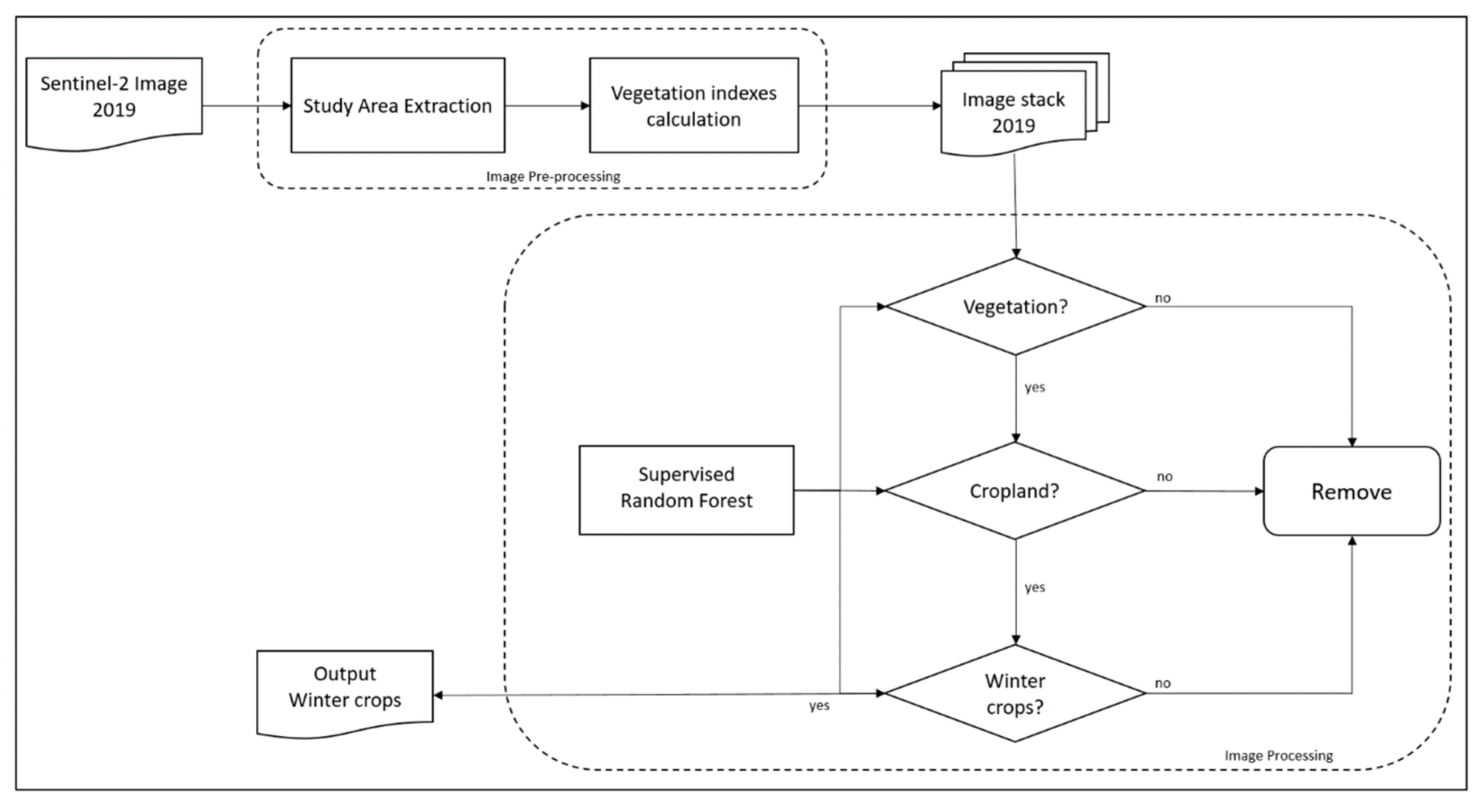
Besides the contributions of the new generation of EO data, the diversity of the classification approaches and methods have provided more resources for agriculture mapping and monitoring. The classical, direct extraction approach is the traditional and most used classification approach that is used to extract single or multiple crop types directly from satellite images [12,13,14]. Moreover, we also propose the hierarchical classification approach for crops mapping in this study. Hierarchical classification is well known for its capacity to solve a complex classification problem by separating the problem into a set of smaller progressive classifications; it produces a series of thematic maps to progressively classify the image into detailed classes. Wardlow and Egbert [12] investigated the applicability of time-series Moderate Resolution Imaging Spectro-radiometer (MODIS) 250 m normalized difference vegetation index (NDVI) data for large-scale crop mapping in the Central Great Plains of the U.S. The hierarchical classification scheme was applied in this study with high classification accuracy, and instead of directly solving a complex irrigated crop mapping problem, a four-level hierarchical classification framework was implemented to produce a series of crop-related thematic maps that progressively classified cropland areas into detailed classes. Ibrahim et al. in 2021 [15] have also employed the hierarchical classification scheme to map crop types and cropping systems in Nigeria, using the RF classifier and Sentinel-2 imagery. Firstly, they produced a land cover map with five classes in order to eliminate other land cover types, then the next classification was performed only on cropland, where the specific crop types and cropping systems were mapped. The results indicated that the crop types were well classified with high accuracy, despite the study area being heterogeneous and smallholder-dominated.

In recent years, most studies in the agricultural field have explored the performance of different classification algorithms. Random Forest (RF) is one of the most well-known and widely used algorithms in the field for its optimal classification accuracy, effectiveness on large data bases, and its capability of estimating the importance of the variables in the classification [8,16,17,18,19]. The RF classification algorithm is traditionally run as a Pixel-Based Classification, which has proven efficient and accurate in agriculture fields by many studies [16,20,21,22]. On the other hand, the advantage of Object-Based Classification (OBC) is well documented and many recent studies have the conclusion that OBC usually outperforms PBC for its higher classification accuracy, better potential for extracting land cover information in a heterogeneous area with small size field, and the capacity to produce a more homogenous class [23,24]. However, even though Object-Based Classification is better developed and considered as more accurate than PBC, both classification methods are able to achieve a great degree of accuracy.

Aside from mapping and analyzing the crop spatial distribution, understanding agricultural growing patterns is also a key element for crop management. Crop phenology monitoring and the identification of the main phenological stages are highly necessary for agricultural production predicting, efficient interventions of farmers and decision-makers during the phenological phases such as fertilization, pesticide application, and irrigation [25]. In particular, germination is the most critical phase to be understood, and it is the starting point of the growing season. Based on the germination information, the farmer and decision-makers are able to make a future projection of the season, estimate the whole seasonal phenology for crop growth, and predict its production [25]. Furthermore, phenology is highly related to the seasonal dynamics of a growth environment, therefore, in the context of global warming, the phenology of many plants, especially crops, may have changed [6].

Crop phenology is usually monitored with optical satellite images using vegetation indices. For example, Pan et al. in 2015 [26] analyzed the phenology of winter wheat and summer corn in the Guanzhong Plain in the Shanxi Province, China by using Normalized Difference Vegetation index (NDVI) time series data and extracted seasonality information from the NDVI time series for measuring phenology parameters. The potential of another less-known index, the Normalized Difference Phenology Index (NDPI), is exploited by Gan et al. in 2020 [27] in order to detect winter wheat green-up dates. During the evaluation with three other indices (NDVI, EVI, and EVI2), the results indicate that NDPI outperforms the other indices with the highest consistency with the ground truth.

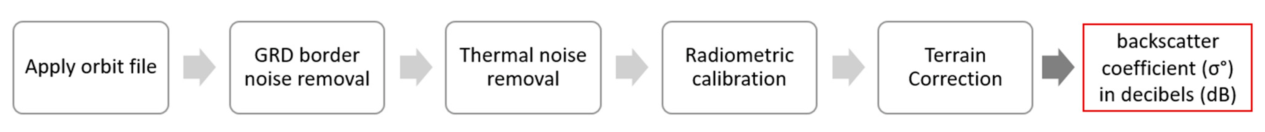
Compared to the optical data, SAR data is less used in agricultural areas. Nevertheless, lately, with the emergence of a new generation of high-resolution SAR data, in particular since the Copernicus program Sentinel-1 C-band high spatial–temporal resolution images became available, SAR data has begun to draw interest, especially for its advantage of having its own source of energy, making it nearly independent of weather conditions [8]. Thus, SAR backscattering coefficient time series data is now more frequently used for crop phenology monitoring. While optical data strongly depends on the chlorophyll content in the plants, SAR data can reveal the main changes in the canopy structure, identify significant phenological stages, and determine the main growing period with the signal that is received after interacting with the canopy of the plants. Therefore, studies of crop phenology monitoring using SAR data have increased considerably in recent years. Meroni et al. in 2020 [28] conducted a study of retrieving the crop-specific land surface phenology (LSP) of eight major European crops from Sentinel-1 SAR and Sentinel-2 optical data, where crop phenology was detected on the temporal profiles of the ratio of the backscattering coefficient VH/VV from Sentinel-1 and NDVI from Sentinel-2. They revealed that the crop phenology that was detected by Sentinel-1 and 2 can be complementary. Wali et al. in 2020 [29] introduced rice phenology monitoring in the Miyazaki prefecture of Japan by using Sentinel-1 dual polarization (VV and VH) time series data, and attempted to clarify the relationship between rice growth parameters and the backscattering coefficient using the combination of two linear-regression lines. Canisius et al. in 2018 [30] exploited SAR polarimetric parameters that were derived from fully polarimetric RADARSAT-2 SAR time series data to predict the growth pattern and phenological stages of canola and spring wheat in the Nipissing agricultural district of Northern Ontario, Canada. Mandal et al. in 2020 [31] proposed a dual-pol radar vegetation index (DpRVI) from Sentinel-1 difference data (VV-VH) to characterize the vegetation growth of three crop types (canola, soybean, and wheat) from sowing to full canopy development, with the accumulation of the Plant Area Index (PAI) and biomass.

The feasibility and effectiveness of winter crop type mapping and phenology monitoring with optical or SAR satellite data has been proven by many studies in agricultural field, however, some limitations remain. For example, the potential of a vegetation index other than NDVI and EVI has rarely been explored, and the studies have never been performed in a coastal area with fragmented and small-scale fields. More importantly, almost all the research perform and evaluate a single classification approach or method, instead of comparing different approaches and methods for crop type mapping.

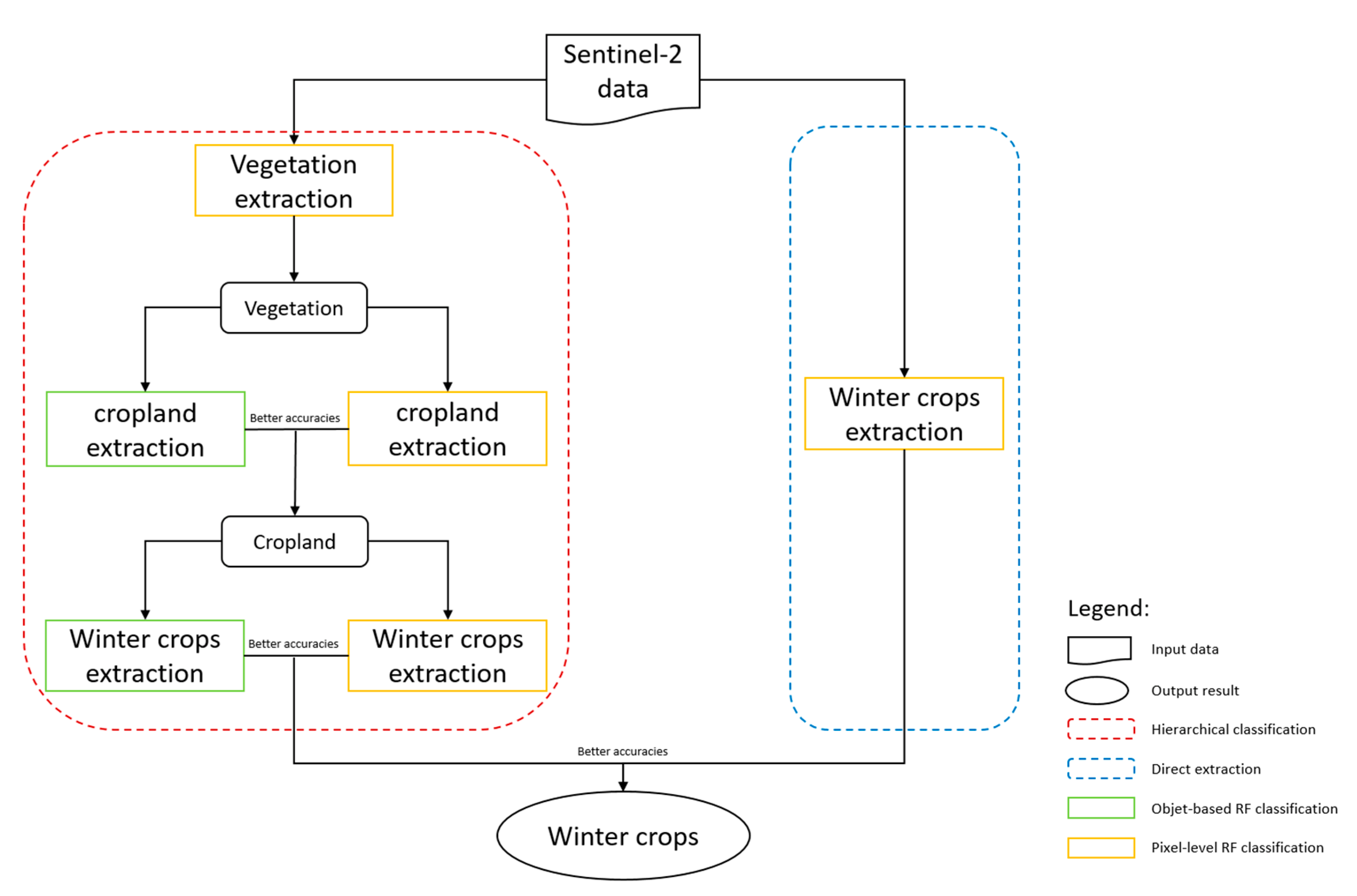
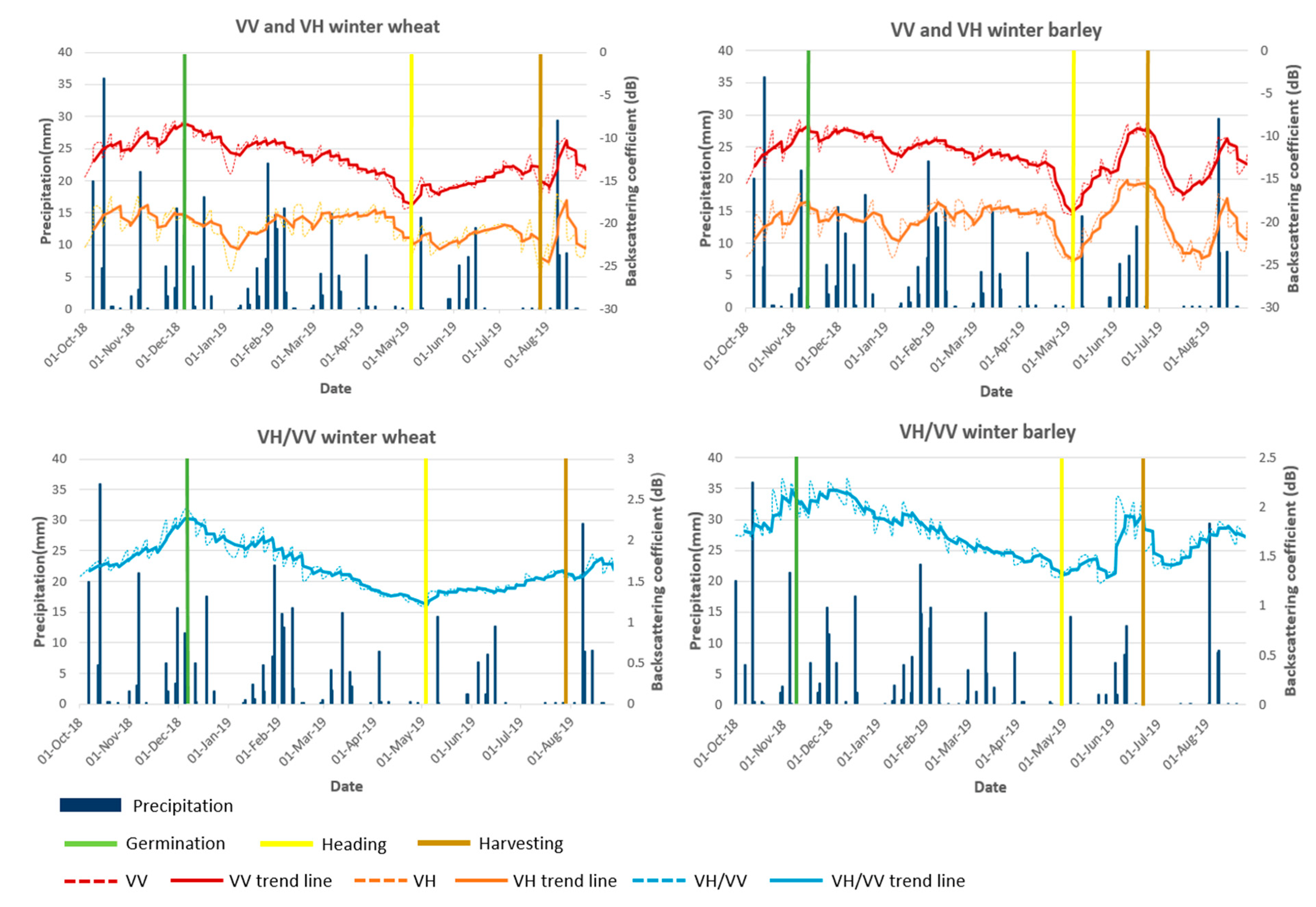
In this study, we introduce a methodology to map two winter crop types (winter wheat and winter barley) with Sentinel-2 optical data that was acquired during the growing season of the winter crops. Two different classification approaches (hierarchical classification and classical direct extraction) were performed using RF-supervised classification algorithms, and two classification methods (PBC and OBC) were operated and evaluated within the hierarchical classification framework. With the classification results of the winter crops, we are able to monitor their phenology with Sentinel-1 C-band SAR backscatter time series and precipitation data in order to understand their temporal behavior from sowing to harvesting, identify the three main phenological stages (germination, heading, and ripening, including harvesting), and study how crop phenology responds to weather conditions.

The main objectives of this study are listed as follows:

• Study the feasibility of mapping winter crops with Sentinel-2 10 m spatial resolution data in a fragmented area that is dominated by small-size fields;
• Perform hierarchical classification and classical direct extraction and evaluate the performance of both classification approaches;
• Perform PBC and OBC and compare the performance in each level of the hierarchical classification structure;
• Study the correlation between crop phenology and Sentinel-1 C-band SAR backscatter time series data and identify three phenological stages and the main growth period of the winter crops.

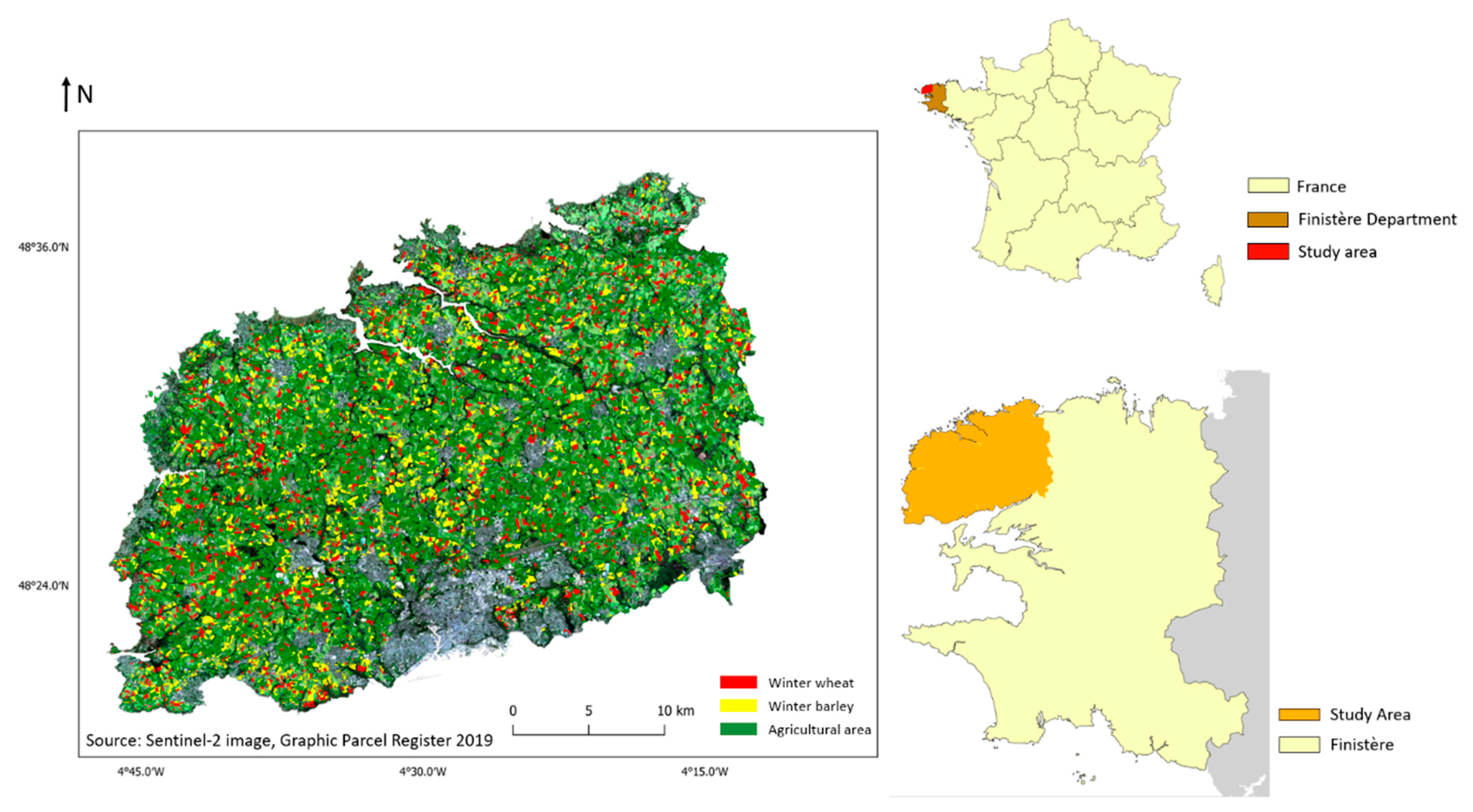
2. Study Area

The study area is located on the west coast of France in the north of the Finistère department and the region of Brittany (Figure 1).

The study area covers a land surface of 1034.41 km², and extends between the latitudes of 48°19′39″N and 48°40′41″N, and the longitudes of 4°12′50″W and 4°47′13″W. According to French National Institute of Geographic and Forest Information (IGN), the northern part of Finistère is mostly dominated by plains, and the elevation of the area ranges between 0 m and 100 m [32]. The study area is mostly occupied by cropland, temporal or permanent grasslands, small area of forests and shrubs, urban agglomeration in the south, and a wetland area in the north [33]. Climatically, the north of Finistère is classified as type Cfb (temperate oceanic climate), according to the Köppen climate classification, and it is characterized by warm winters and cool summers. On average, the northern region of Finistère receives 941 mm of total precipitation per year, with the annual average temperature being 12.1 °C (7.7 °C and 16.8 °C are the monthly average temperatures for the coldest and warmest months, respectively), and therefore the warm temperate climate with frequent rainfall provides very favorable conditions for agriculture activities.

With such climate and topography conditions, agriculture is an important economic sector in the study area, and a considerable number of locals work in an agricultural or related sector in the department. There are 384,408 hectares of useful agricultural area in the department, so 57% of the department’s surface is devoted to agricultural use [34]. One of main agricultural productions are crops, including corn, winter wheat, and winter barley, and vegetables [35].

Hence, it is important to develop a methodology to map one or several specific crop types and monitor their growth stages by using free access, high quality satellite images for crop production management. The north of the Finistère department was chosen as our first study area because of its favorable natural conditions, highly active agricultural activities, and its proximity, which facilitate the field research and interaction with farmers.

3. Data

The study was executed in the Finistère department in France during 2019, using open-access high-quality satellite data from the Sentinel platform. It is worth noting that the latest version of the graphic parcel register was published in 2019 by the French National Institute of Geographic and Forest Information, and this information was relevant to our study.

Due to the annual high-intensity precipitation there is frequent heavy cloud cover in the region, therefore, operable optical satellite images are very rare in the study area. Nevertheless, a Sentinel-2 optical satellite image was acquired in the spring, which is the growing season of the winter crops. In order to create a cloud-free time series of the study, the phenological phrases of winter crops from the SAR data were applied to the phenology monitoring process.

3.1. Sentinel-2 Optical Data

Sentinel-2 is an satellite imaging mission that is implemented by the European Commission (EC) and the European Space Agency (ESA) as a part of the Copernicus program [36]. The two identical satellites (Sentinel-2A and Sentinel-2B) provide continually open-access, multispectral, wide swath (290 km), high spatial resolution (four bands at 10 m, six bands at 20 m, and three bands at 60 m), and high revisit frequency (five days with combined satellites) image data [36]. Due to frequent heavy cloud cover in the area, only one cloud-free level 2A atmospheric effect-corrected Sentinel-2 image from 20 April 2019 was acquired from the Theia platform (catalog.theia-land.fr) [37] (

Table 1. Sentinel-2 image used in the study.

Date	Satellite	Platform	Processing Level	Tiles
20 April 2019	Sentinel-2	2B	Level 2A	T30UUU

). Ten spectral bands (

Table 2. Sentinel-2 spectral bands used in the study.

Sentinel-2 Bands	Spatial Resolution (m)	Wavelength Range (nm)
Band 2-Blue	10	458–523
Band 3-Green	10	543–578
Band 4-Red	10	650–680
Band 5-Vegetation red edge	20	698–713
Band 6-Vegetation red edge	20	733–748
Band 7-Vegetation red edge	20	773–793
Band 8-Near Infrared	10	785–899
Band 8A-Vegetation red edge	20	855–875
Band 11-Short-Wave Infrared	20	1565–1655
Band 12-Short-Wave Infrared	20	2100–2280

) were extracted for further processing and analysis.

3.2. Sentinel-1 SAR Data

The Sentinel-1 C-band SAR (Synthetic-aperture radar) is one of the ESA missions under the Copernicus program [38]. Sentinel-1 possesses two polar-orbiting satellites (Sentinel-1A and Sentinel-1B) sharing the same orbital plane, which are able to operate day and night using their own energy source in order to perform high spatial resolution (10 m), wide coverage, high repeat cycle (generally five days with two satellites), C-band SAR imaging in all weather conditions [38].

In this study, interferometric Wide Swath mode level-1 GRD (Ground Range Detected) Sentinel-1 data with an incidence angle ranging from 30 to 46 were acquired to create the time series of the growing period of the winter crops (winter wheat and winter barley) in 2019, from 1 October 2018 to 1 September 2019. Both polarizations (VV + VH) were used, but only the descending orbit was retained for the processing. In total, 109 Sentinel-1 C-band SAR images with descending orbit were acquired for this study.

3.3. Auxiliary Data

RPG (Graphic Parcel Register) was applied as the ground truth data in our study, used for creating training data and test data. RPG 2019 is the latest version of the very precise, geo-referenced agricultural land database that covers the entire France territory (except Mayotte) that was published by IGN. The databases show the precise crop types (e.g., wheat, corn, vegetables, sunflower) or temporary and permanent grasslands in that are in the recorded agricultural lands in each year [39].

4. Methods

The methodology of this paper is detailed in two parts, which relate to the two research subjects: mapping winter crop types using Sentinel-2 data, and monitoring crop phenology with Sentinel-1 backscatter time series. The data were processed in QGIS with Orfeo Toolbox, eCognition 10.0, and GEE (Google Earth Engine).

4.1. Winter Crop Types Mapping

A flow chart of the proposed global methodology is displayed below (Figure 2)

4.1.1. Image Preprocessing

After the study area selection and satellite image acquisition, the boundary of the northern region of Finistère area was applied in order to extract our area of interest by subsetting the raw images for the purpose of reducing the image size and shortening the processing time.

In remote sensing fields, vegetation indices (VI) are the qualitative and quantitative evaluation of vegetation covers and their growth dynamics, using different combinations of spectral measurements. The results of the indices are different due to the different chemical and morphological characteristics of the surfaces of the organs or leaves of the plants [40], however the spectral responses are also affected by other factors, such as environmental effects, soil reflectance and its components, shadows, and atmospheric and topographic effects [41].

For this reason, over a hundred VIs have been developed and enhanced for various applications over the past three decades in order to enhance spectral responses, increase sensitivity for identifying vegetated areas, distinguish different vegetation types, evaluate the vegetation density, and provide data on the health of the vegetation [42], and also to minimize the effects of other factors that are described above [41]. In this study, six VIs are used with the aim of mapping winter crop types using Sentinel-2 data.

• The Normalized Difference Vegetation Index (NDVI), proposed in 1973 by [43], is the most known and widely used index in research related to vegetation monitoring. NDVI is the normalized difference between the visible red and near-infrared spectral reflectance of vegetation, as follows:

$$NDVI=\frac{NIR-RED}{NIR+RED}$$

(1)

Even though the index is often affected by atmospheric conditions and soil reflectance and its components, it remains a highly used index in agriculture-related fields to measure the rate of vegetation cover and evaluate the health of the crops.

• The Normalized Difference Water Index (NDWI), proposed by Gao in 1996 [44], is a vegetation index that is used to highlight the changes in the liquid water content of vegetation canopies with weak atmospheric aerosol scattering effects, while remaining independent of the soil background [44]. The index is the normalized ratio between visible red and short-wave infrared spectral bands, and the expression of this is displayed below:

$$NDWI=\frac{NIR-SWIR}{NIR+SWIR}$$

(2)

With its high sensitively to water stress, NDWI is frequently used for the agricultural monitoring of drought and irrigation management. As well, some studies reveal the possibility of distinguishing crop types, especially winter crops, with NDWI [20,45,46,47].

• The Green Normalized Difference Water Index (GNDVI) was proposed in 1996 by Gitelson et al. [48], as NDVI; it is the index for evaluating the photosynthetic activity of the vegetation, except that the visible red band is replaced by the green band, ranging from 0.54 to 0.57 microns, and the expression of it is as follows:

$$GNDVI=\frac{NIR-Green}{NIR+Green}$$

(3)

Besides NDVI, the “Green” NDVI is more sensitive for assessing the chlorophyll concentration at the canopy level and it enables a precise estimation of the pigment concentration [48].

• The Enhanced Vegetation Index (EVI), developed by the MODIS Land Discipline Group [49], is aimed at optimizing the vegetation signal and correcting the imprecision of NDVI with improved sensitivity in high biomass regions by appending several additional spectral bands [50], and it is calculated by the following equation:

$$EVI=\frac{G\ast \left(NIR-Red\right)}{\left(NIR+C1\ast Red-C2\ast Blue+L\right)}$$

(4)

EVI is able to reduce the atmospheric conditions and canopy background noise with high sensitivity in densely vegetated areas and it is more responsive to canopy structural variations as compared to NDVI [50].

• The Soil-Adjusted Vegetation Index (SAVI), was proposed by Huete in 1988 [51] as an attempt to improve NDVI, which is frequently affected by the soil background conditions. Therefore, the index aims at minimizing the influence of soil brightness and eliminating the need for the additional calibration for different soils by using a soil-brightness correction factor [51]. It has an adjustment factor (L) in its calculation:

$$SAVI=\frac{\left(NIR-Red\right)}{\left(NIR+Red+L\right)}\left(1+L\right)$$

(5)

SAVI was found to be helpful in separating different crop types, especially spring crops from winter ones [52].

• The Modified Soil Adjusted Vegetation Index (MSAVI) was developed by [53] in 1994 as an improved version of SAVI, with the constant soil adjustment factor L being replaced. It is proven to increase the dynamic range of the vegetation signal while further minimizing the soil backgrounds spatial and temporal variations, therefore resulting a greater vegetation sensitivity:

$$MSAVI=\frac{\left(2\ast NIR+1-\sqrt{{\left(2\ast NIR+1\right)}^2-8\ast \left(NIR-RED\right)}\right)}{2}$$

(6)

Studies have proven that MSAVI can be used in the agriculture field [54,55], and even more in winter crop monitoring [56].

After calculating the vegetation indices, an image stack with the ten original spectral bands and all of the indices was created for further image processing.

4.1.2. Image Processing

In this study, for the better extraction of winter wheat and winter barley in the study area from the satellite image, supervised image processing using different approaches was performed in order to make comparisons and attempt to reach the most adapted classification in this study (Figure 3).

Compared to the direct extraction of winter crops with pixel-based RF algorithms, hierarchical classification methods are effectuated in three progressive levels, each with different objectives. The objectives from the first level of the hierarchy to the last one are extracting vegetation (including croplands) from raw images, extracting croplands from vegetated areas (trees, shrubs, and grassland), and finally, obtaining exclusively winter wheat and winter barley from all crop types detected in previous stages, respectively. Finally, the results of the two classification approaches were evaluated with accuracy indices, in order to distinguish which one had better agreement with the ground truth data.

In addition, inside the hierarchical classification structure, except for during the first step, separating vegetation and non-vegetation exclusively used the pixel-based RF algorithm and this reached a very close agreement with ground truth data. Each step has been performed using the two methods, pixel-based and object-based RF classification, in order to determine the result with better accuracies for further processing and analysis.

Pixel-Based Classification (PBC)

The traditional PBC is the most used method in remote sensing, especially for land use classification; therefore, this method was also widely employed in this study. The PBC was done on the pixel level, which is the smallest unit in an image, where only the spectral information of each single pixel was used. During the classification, each pixel was assigned predefined classes by using a model that was well trained with training data and a classification algorithm. In this paper, PBC is performed in both classification approaches.

Object-Based Classification (OBC)

OBC starts with an additional processing step before classification, which involves the segmentation of an image into numerous, non-overlapping, homogeneous objects [23], hence, the OBC was done on the object level instead of the pixel level. At the same time, aside from the simple spectral information, the texture, color, form, and size of the objects are taken into account. Later the individual object that was generated by the segmentation algorithm was used for classification.

A Multiresolution Segmentation (MRS) algorithm was applied as the first step of the object-based image analysis (OBIA) in the current study. This relatively complex and user-dependent algorithm has proven to be one of the most successful image segmentation algorithms in the OBIA area [57]. At the beginning of the process, each pixel is considered as a segment; afterwards, pairs of adjacent image objects are merged to form larger segments [58]. The three main parameters of the algorithm: scale, shape, and compactness, can be adjusted by users. The scale parameter is able to define the maximum standard deviation of the heterogeneity in order to control the amount of spectral variation within objects and the size of their results [57,59]. Thereafter, there are also two homogeneity criteria, the shape criterion that defines the weight between the shape and the spectral information of the objects, and the compactness criterion which represents the compactness of the objects during segmentation [60].

In this study, several combinations of parameters were used, and the optimal ones were found on a trial-and-error basis. The scale, compactness, and shape parameters were assigned as follows: 15, 0.5, and 0.3, respectively, for cropland extraction, and 20, 0.5, and 0.1, respectively, for winter crops extraction.

Supervised RF Classification

Supervised RF classification was performed on the Sentinel-2 data. It is the most common procedure for the quantitative analysis of remote sensing imagery [61], and it involves the use of training data for machine-learning classification. The training data were selected with reference data, knowledge, and experience provided by the user, and the selected samples were considered representative of each class.

Training data and test data in our research were selected in this step, using the RPG 2019 map. For the purpose of comparing different methods of classification, training data that were selected for PBC and OBC were as similar as possible, such as using the same area and very approximate surfaces, in order to improve the global comparability of the two methods.

RF classification has been one of the most known and widely used classification algorithms, especially in the land cover classification field, over the past two decades. This powerful machine learning classifier has numerous key advantages, such as a low sensitivity to noise or overtraining, the ability to handle high-dimensional data, its high classification accuracy and non-parametric-nature, and its capacity to determine variable importance [19].

RF is also one of the ensemble learning algorithms that builds numerous classifiers that have been proven to improve classification accuracy considerably. For classification, RF forms an ensemble method using a tree-like classifier, where each tree in the forest contributes a single vote for the most popular class, and the majority of the vote determines the final prediction of the RF model [62].

The training and classification of the RF module were applied using the Orfeo toolbox with two user-defined parameters that were set on a trial-and-error basis: the number of decision trees grown in the forest and the maximum tree depth, which is the length of each tree in the forest. The two parameters that were used in this study were defined as 100 and 25, respectively.

4.1.3. Image Post Processing

After the classification, the accuracy assessment was performed with test data in order to evaluate the classification’s degree of agreement with the reality and therefore assess the reliability of the classified results. In this study, in order to evaluate the classification quality and compare it amongst the different classification methods, five well-known and highly promoted accuracy indices were calculated for each classification method and each class. Among them, overall accuracy (OA) and kappa were employed for the global accuracy assessment, otherwise, precision, recall, and F-score were computed to assess the classification results of each class.

The OA is one of the traditional measures of classification accuracy that is derived from the confusion matrix [63]. It indicates the probability that an individual pixel will be correctly classified by a classifier [64], hence, it is computed by dividing the number of correctly classified pixels by the total number of pixels in the confusion matrix. The popular kappa coefficient was first applied in the remote sensing community to express the classification accuracy in the early 1980s [65], and it is considered to be the assessment of the inter-classifier agreement and the accuracy of two classifiers; it usually gives a statistically more sophisticated measure of interclass agreement, also it gives a better interclass discrimination than OA does [66].

Among the per-class accuracy assessments, precision and recall were computed from the confusion matrix as well. Precision is also called the positive predictive value, which is related to the rate of correct positive predictions among the total predictions that are classified as positive, and the recall or sensibility represents the rate of the actual positive individual pixels that are correctly detected by the classifier. Furthermore, the F-score was generated from the precision and recall; it provides a single harmonic mean of the model’s precision and recall.

In the hierarchical classification process, test data that were used for evaluating the classification of each step were generated as random points from the image that were used to perform classification, which is the result of the previous steps. Afterwards, the random points were labelled manually with the Graphic Parcel Register map as ground truth. However, with the aim of evaluating the performance of the proposed hierarchical classification approach by comparing with traditional direct extraction, a completely new test dataset was produced from the original Sentinel-2 image that was not classified.

4.2. Crops Phenology Monitoring

This second part of the study was performed, based on the mapped winter crops from the previous step. Due to limited climate conditions in the study area, winter crop phenology monitoring was performed with Sentinel-1 C-band SAR data using the Google Earth Engine (GEE) platform. GEE is an open-source, cloud computing platform with a fast, high-performance computation and visualization system and a large data catalog which hosts a large repository of publicly available geospatial datasets, including a variety of satellite imaging systems [67]. The platform is designed for global-scale geospatial big data storage, processing, and analyzing [68]. The utility of GEE has been examined in different fields, for vegetation mapping and monitoring, land cover change mapping, and agriculture applications [68].

The platform proposes a complete data process chain from a single or a collection of analysis-ready images to library functions or user-defined algorithms that are applied to achieve results generation and visualizing. One of its main advantages is allowing long- term monitoring using a user-defined period with free access to preprocessed time series data. Hence, in this study, the backscatter coefficient (σ°) in decibels (dB) of both polarizations (VV and VH) and their ratios of a Sentinel-1 image time series during a complete growing period of winter crops (from October to September) on a few chosen croplands was automatically generated in a line chart on the GEE platform. In order to study the scattering behavior of our target croplands, each image was preprocessed, and the backscatter coefficient was converted to dB by GEE using the Sentinel-1 Toolbox (Figure 4) A flow chart of the Sentinel-1 image time series process in GEE is displayed as follow (Figure 4):

The first step in applying the orbit file aims at updating the orbit metadata with a restituted orbit file, then Ground Range Detected (GRD) border noise removal attempts were performed to remove the low intensity noise and invalid data on the scene edges. Afterward, a thermal noise removal function aims to remove the additive noise in sub-swaths to reduce the discontinuities between sub-swaths for scenes in different acquisition modes. Thereafter, radiometric calibration is applied to compute the backscatter intensity, and subsequently, a terrain correction, also called an orthorectification, was performed to convert the data from ground range geometry to σ° [69]. Lastly, dB was calculated from σ° with the equation dB = 10 × log10σ°. A series of line charts in dB were plotted for each polarization and ratio of each winter crop.

5. Results

5.1. Winter Crop Types Classification Methods Comparison

The classification results of the different approaches and methods of the winter wheat and winter barley and their accuracy analysis are presented in this part. Firstly, the results of PBC and OBC of each step in the hierarchical classification are demonstrated and evaluated through accuracy assessments, the more accurate results were retained for further processing and comparison with classical direct extractions. Then the final results of the hierarchical classification and classical direct extraction are displayed and compared with accuracy assessments as well.

5.1.1. PBC versus OBC

Vegetation Extraction

For vegetation extraction (including cropland), only PBC was performed since it achieved a great accuracy, approximately close to 1. From Figure 5 we see that the distribution of vegetation and cropland is coherent in the study area, apart from some urban environments, which are marked by intense non-vegetation pixels, in particular these areas are in the south and the northeast of the study area. According to

Table 3. Accuracy assessment of PBC vegetation (including cropland) extraction.

	Precision	Recall	F-Score
Vegetation	0.992	0.997	0.995
Non-vegetation	0.994	0.984	0.989
Kappa:	0.984
Overall accuracy (OA):	0.993

, both global and interclass accuracy indices are very close to 1, this indicates a high probability of a correct classification of each individual pixel, and a great overall agreement level with the ground truth. Besides a good performance and good training of the PBC method, the distinction between the vegetated area and non-vegetation is very significant, and therefore, it is easy to classify.

Croplands Extraction

Subsequently, based on the vegetated area that was extracted from the previous step, we aimed to distinguish and preserve only the croplands from all arboreal vegetation, shrub, and grasslands, including pasture. In this step, OBC and PBC were both performed and evaluated. Figure 6 demonstrates that the results of the two methods are almost identical, although more individual pixels were classified as cropland in PBC considering that PBC was operated on pixel-level.

Pursuant to

Table 4. Accuracy assessment of OBC croplands extraction.

	Precision	Recall	F-Score
Vegetation	0.786	0.746	0.765
Cropland	0.912	0.905	0.908
Others	0.700	0.875	0.778
Kappa:	0.716
Overall accuracy (OA):	0.861

and

Table 5. Accuracy assessment of PBC croplands extraction.

	Precision	Recall	F-Score
Vegetation	0.769	0.678	0.721
Cropland	0.879	0.932	0.905
Others	0.929	0.813	0.867
Kappa:	0.692
Overall accuracy (OA):	0.857

, even though the global accuracy indices of the results of OBC are slightly better than PBC with a difference of 0.024 in kappa and 0.004 in OA, the indices of the two results are still comparable. The tables below show that a large proportion of pixels are correctly predicted, in general, and that the level of agreement with the ground truth data is somewhat lower, but it is still acceptable. Furthermore, for the interclass accuracy evaluation, cropland generally has the highest precision, recall, and F-score results, which are all around 0.90. The models were well trained to make a good prediction of the cropland class, especially for the OBC model, and most of the individual pixels belonging to the cropland class were correctly detected. This can be explained by the OBC taking into account the geometry, form, and texture elements, which are the key elements that are used to distinguish the croplands from other vegetation. The classification of the vegetation has a slightly lower accuracy of approximately 0.2 in comparison with croplands because of the mix of different kinds of vegetation and the uncertain form of the vegetated area, though OBC remains more precise when it is compared to PBC. Finally, the classes of the other pixels in our study area, which were mainly some isolated pixels that were left from the previous step due to some errors, were better classified with PBC since the non-vegetated area has highly different spectral behavior as compared to that of vegetation. Considering the better accuracy assessments of OBC, its classification result was preserved to perform the next step of classification.

Winter Crops Extraction

In this final step, two winter crop types were extracted, based on the results of the previous step, and the classification result of the cropland extraction was achieved by using OBC. The results of the two classification methods (Figure 7) are very close to identical in this level, wherein the differences between the two maps can hardly be noticed.

With the lack of a possibility to visually compare the two methods, they were evaluated and compared by using accuracy assessments (

Table 6. Accuracy assessment of OBC winter crops extraction.

	Precision	Recall	F-Score
Winter wheat	0.998	0.978	0.988
Winter barley	0.833	0.871	0.852
Other crops	0.870	0.848	0.859
Kappa:	0.848
Overall accuracy (OA):	0.899

and

Table 7. Accuracy assessment of PBC winter crops extraction.

	Precision	Recall	F-Score
Winter wheat	0.994	0.976	0.985
Winter barley	0.876	0.913	0.894
Other crops	0.917	0.895	0.906
Kappa:	0.892
Overall accuracy (OA):	0.928

). In regard to the global accuracy indices, all classes were stated as accurate when using the two methods, which signifies a good performance by both methods with a high accuracy and a strong level of agreement for the classification. Beyond that, it is worth noticing that PBC shows a better potential with about 0.03 higher value in the OA and 0.04 in kappa, moreover, PBC basically achieves a better accuracy indicator of three classes in comparison with that of the OBC. The results illustrate that the difference in spectral behavior was exploited to distinguish winter crops from other crops, since all the croplands share similar geometry, form, and texture characteristics. Nonetheless, among the different crop types that were presented in our area of study, winter wheat has the most distinctive spectral signature, thus it was found to be the class with the best accuracy indices in both results, with very strong reliability in terms of prediction and a high rate of precisely identifying winter wheat. In contrast, the classification of winter barley and other crops are somewhat less accurate with approximately 0.1–0.5, and the advantage of PBC is more significant, with higher accuracy indicators of around 0.04, which might be caused by the confusion of winter barley and other crops due to the similarity of their spectral behavior. In addition, the difference between these two classes were better detected by PBC with spectral information.

5.1.2. Hierarchical Classification versus Classical Direct Extraction

The results of the hierarchical classification, which is the classification approach that was proposed in this study, and the classical direct extraction for the winter crops mapping are presented in Figure 8. Generally, winter wheat and winter barley were well detected and extracted from the Sentinel-2 image; the results of two classification approaches are globally identical, with particular reference to the homogeneous distribution of the winter crops over the area of interest. Nevertheless, the classical direct extraction approach identified more winter croplands, especially winter barley, and the winter croplands that were detected are much more fragmented; many small pixels were classified as croplands. This could be explained by the fact that winter crops are directly extracted from the preprocessed image; in addition, there might be some confusion between winter barley, grasslands, and some different crops considering the resemblance of their spectral behavior.

To make a better comparison, the accuracy assessments of the two approaches are displayed in

Table 8. Accuracy assessment of hierarchical classification.

	Precision	Recall	F-Score
Winter wheat	0.991	0.904	0.946
Winter barley	0.886	0.900	0.893
Others	0.929	0.959	0.944
Kappa:	0.888
Overall accuracy (OA):	0.932

and

Table 9. Accuracy assessment of classical direct extraction.

	Precision	Recall	F-Score
Winter wheat	0.959	0.928	0.943
Winter barley	0.683	0.960	0.799
Others	0.955	0.797	0.869
Kappa:	0.789
Overall accuracy (OA):	0.866

. According to the tables, both classification results are very satisfactory as mostly all of the accuracy indicators range from 0.8 to 1, specifically, with the hierarchical classification, almost all indices are superior to 0.9. This suggests a good performance and training of the models and also a strong agreement with ground truth of all classification approaches in the study. Still, it is worth noticing that the hierarchical classification shows a better potential for specific crop type mapping as compared to the classical direct extraction (approximately 0.1 higher in kappa and 0.07 in OA). Additionally, nearly every class achieved a higher accuracy in hierarchical classification, which indicates that the model is solid, and it is able to make a good prediction. Among the three classes, winter wheat is the most correctly classified class in both of the classification approaches, the indicators that range from 0.90 to 0.99 and with an F-score that is highly similar. Hierarchical classification reaches a better precision index, that means that the model is more exact, yet classical direction extraction achieved a finer recall, which means that the model returned more relevant results, and it can correctly and efficiently identify winter wheat. In addition, winter barley and the other classes were evaluated and less accurately classified, especially with the classical direct extraction approach. According to Table 8, the winter barley class obtained a high recall (0.960) and a relatively lower precision (0.683), which suggests a high false-positive rate; many individuals that were predicted as winter barley that the model returned were found misclassified when they were compared to the test data. On the contrary, the other class received a high precision index (0.955) and a comparatively low recall (0.797), and these indicators demonstrate that the pixels were correctly detected and labelled despite there being fewer results returned by the model. The comparably low accuracy of the two classes and the imbalance between the precision and recall indices might be explained by: (1) the similarity of the spectral behavior between winter barley and other crops and even grassland in the case of the classical direct extraction approach. (2) Since two winter crops are extracted directly from the Sentinel-2 image, the other class included not only non-vegetated urban areas, but also vegetation and other croplands which occupy a large area of our study site. Therefore, an imbalance between classes was caused, thus, more training datasets of the other class were acquired in consideration of its weak intraclass correlation.

5.2. Crops Phenology Monitoring

The Sentinel-1 temporal backscattering coefficient profiles of diverse land cover types at VV and VH dual-polarizations from the study area during the growing season of the winter crops (from 1 October 2018 to 1 September 2019) are shown in Figure 9; the temporal profiles of the mean σvv and σvh values of urban, vegetation (including other crops), water, bare soil, winter wheat, and winter barley land cover are displayed. As shown in Figure 9, besides the profiles of the water area, which fluctuate significantly due to the weather conditions, the temporal profiles of the vegetation, urban, and bare soil are much more stable than the profiles of winter crops are, which have a significant fluctuation according to their different growth stages. Especially in the σvh profile, the vegetation, urban, and bare soil profiles are generally close to their mean value, regardless of the season. Nonetheless, the variation of the backscattering coefficients of the two winter crops are clearly evident, for example, a peak is seen in early December, followed by a minimum value in early summer and a maximum value in midsummer. Thus, the results indicate that it is feasible to distinguish winter crops from other types of land cover, particularly vegetation and other crops, and furthermore, we are able to identify and study the main phenological stages from germination to ripening (harvesting) by using Sentinel-1 temporal profiles.

Based on prior knowledge and field research with local farmers, winter wheat and winter barley are both cereal crop types that are planted from October to November. Generally, winter barley is sowed earlier than winter wheat in the Finistère department. Germination, which is the first growth stage of the crops, takes place three to four weeks after sowing, hence, this is in early December for winter wheat and in mid-November for winter barley. The crops remain in their vegetative stage during winter, and stem elongation begins in spring, and it lasts until the plants reach their maximum height, usually in early summer. Lastly, ripening, the final growth stage, and harvesting occur in summer (early summer for winter barley and mid-summer for winter wheat).

In Figure 10, both the raw signal and smoothed trend line of the temporal backscattering coefficient profiles of VV, VH, and the VH/VV ratio for the 2018–2019 growing season are displayed. Looking at the charts, it is shown that large variations occur before the germination due to the interaction between the bare soil and vegetation that is caused by stem-ground double scattering [6,70], while previous research suggests that the fluctuation in the backscattering profiles is mostly induced by changes in soil water content and roughness [6]. Pursuant to previous research, germination as the first stage of emergence of the plant can be recognized as the first maximum value of the profiles before they begin decreasing [25], therefore the germination stage is observed at around 1 December for winter wheat, and in early November for winter barley. Moreover, for winter wheat, this phase is best observed with VV and the VH/VV polarizations as they represent the first peak of the curves; however, the peak is better illustrated at VV and VH polarizations for winter barley. Afterwards the overwintering stage occurs, and the crops remain in their vegetative stage during winter (generally around 1 January); a gentle decreasing and a slight flattening can be observed in the VV polarization curves during this stage for both the crops. Furthermore, a fluctuation of the VV and VH curves of the two crops at around 1 January 2019 is driven by a short pause of rainfall, as the signals are highly affected by the soil water content. The stem elongation stage starts in spring, where the vertical development of the stems and leaves of the plants cause soil scattering attenuation, represented as a continuous and steadily decreasing line, until they reach the heading stage, where the plants achieve their maximum height. After a long decreasing phase, σ° reaches the minimum value of the temporal profiles at the heading stage at around 1 May 2019 for both winter crops, and this stage can be better observed in σvv and σvh/vv for winter wheat phenology, and in σvh and σvh for winter barley. However, the sharp decrease in σvv and σvh at the heading stage, specifically in the profiles of the winter barley might be the result of the relative lack of rainfall that occurred after early April. After heading, the inflorescence emergence, anthesis, grain development, and dough development stages occur. As seen on the graphs the curves start to increase during the flowering and grain development stages. These stages are illustrated by a sharp increase in the winter barley, regardless of the polarization, while by contrast the σvv and σvh/vv of the winter wheat shows a smooth increase. At last, the ripening stage, which is the maturation stage, occurs and the crops are ready to be harvested. This phase is shown as the last peak of the profiles during the growing season, followed by a sharp decrease which is caused by the absence of volume and multiple scattering after the harvesting [25]. As the results show, harvesting, which took place around 1 August 2019, is better demonstrated by σvv and σvh for winter wheat, while the harvesting stage was in late June for winter barley, and it is clearly shown by all polarizations, particularly in VV and VH.

The best polarization for each phenological stage (germination, heading, and ripening (harvesting)) are detailed as follows in

Table 10. The best polarization observed for each phenological stage of winter wheat in the study.

Stage	Polarization	Date	Determination
Germination	VH/VV, VV	Early December	First peak of the temporal series
Heading	VV, VH/VV	Early May	The minimum value after emergence
Ripening (Harvesting)	VV, VH	Around 1 August	Last maximum of the profiles, following by a sharp decrease

and

Table 11. The best polarization observed for each phenological stage of winter barley in the study.

Stage	Polarization	Date	Determination
Germination	VV, VH	Early November	First maximum of the temporal series
Heading	VV, VH	Around 1 May	The minimum after emergence
Ripening (Harvesting)	VV, VH, VH/VV	Around 1 July	Last maximum of the profiles, following by a sharp decrease

. The phenology monitoring of the winter wheat highly relies on VV polarization, while the VH/VV ratio is also very helpful in identifying the germination and heading stages. Otherwise, the VH polarization was used to detect the ripening stage and the harvesting event.

Meanwhile, the phenology monitoring of the winter barley depends more on VV and VH polarizations, which are able to easily identify the three phenological statuses. In addition, VH/VV polarization is also effective for detecting the ripening and the harvesting stages.

6. Discussion

6.1. Hierarchical Classification for Winter Crops Mapping

In this study, two different classification approaches using Random Forest machine learning methods were performed on a Sentinel-2 high spatial resolution satellite image that was acquired in April 2019, which is the growing season of the winter crops, in order to detect and map winter wheat and winter barley in a fragmented area that was occupied by different land categories. One of the main objectives of this paper was to successfully extract winter crops data with the hierarchical classification that was proposed in this study, which allows an efficient winter crop type mapping for a study area with a complex landscape, and to easily distinguish winter crops from other land cover types, especially arboreal vegetation, shrubs, grassland, and other crop types. The results of the hierarchical classification were evaluated with different accuracy indicators (global or interclass) and were finally compared with the traditional direct extraction approach.

Both classification approaches achieved a good accuracy level despite the complex occupation and small cropland size in the region, with an overall accuracy of 0.866 and 0.932 and a kappa index of 0.789 and 0.888 for classical direct extraction and hierarchical classification, respectively. Even though the classical extraction method worked well for winter crop mapping, the accuracy assessment indicates that the hierarchical classification is clearly more accurate and better suited to our study by turning a complex multi-class classification problem into a series of smaller classifications. According to the results that are presented in Figure 8 and the accuracy indicators that are displayed in Table 8 and Table 9, apart from the global accuracy indicators, the hierarchical classification has proven to be reliable, with outstanding performance in the classification of both winter crops classes, particularly the winter wheat.

The hierarchical classification approach is widely used in many different fields, such as for categorization problems [71], biological predictions [72,73], and music genre classification [74,75], meanwhile the concept of solving a complete classification problem step-by-step using agglomerative algorithms plays also an important role in image classification and its efficacy is well known and it is recognized by previous studies [76,77,78,79]. In this study, we proposed a hierarchical classification framework that was constituted by three smaller classifiers for extracting winter crop data, and we have clearly demonstrated the superiority of the hierarchical framework over the classical extraction method.

Additionally, both classifications in this study were performed with supervised RF machine learning methods and highly accurate results were acquired, regardless of the approach or the method. Therefore, RF has proven to be a feasible, well-suited classification algorithm for precisely mapping specific winter crop types from a small-sized field in a complex area.

6.2. Comparison of PBC and OBC

In this work, PBC and OBC were implemented in the two steps of the classification process within the hierarchical classification structure (croplands extraction from all vegetated area, and winter croplands extraction from all croplands). In addition, the two classification models were trained by a similar dataset, and then evaluated using the same test data. The two classification methods are widely known and used, and they are always compared in different fields. OBC provides a method to the satellite image classification, and numerous studies in the remote sensing field it is demonstrated that OBC usually achieves a better classification with different data and in different landscapes over PBC by bringing complementary information other than the spectral signal and turning classification units from pixels to image objects [80,81,82,83]. Whiteside et al. in 2011 [23] indicated that OBC has a better potential for extracting land cover information in a spatially heterogeneous land cover area, while Weih and Riggan in 2010 [24] proposed that OBC produced more homogeneous classes, as the classes that were produced by PBC are more fragmented. Furthermore, many studies have also pointed out that OBC regularly outperforms PBC for crop type mapping and they noted that it has a more efficient calculation time [84,85,86]. However, OBC is limited by segmentation errors, such as over-segmentation and under-segmentation, which bring negative impacts to the classification; consequently, low segmentation accuracy leads to low classification accuracy [79,86,87]. Furthermore, some studies have also revealed that the difference in accuracy values between the two methods decreases or even disappears when the same classification algorithms are applied, or the spatial resolution of the image is increased [88,89,90].

In this work, the results illustrate that each method has its advantage in the classification process. OBC slightly outperformed PBC in cropland extraction as the complementary texture, geometry, and shape information are helpful for cropland detecting. On the other hand, PBC reaches a higher accuracy in winter crops extraction, since all croplands have a similar shape, but winter crops can be easily distinguished from other crops with direct spectral information. Additionally, the statistical difference between the results of PBC and OBC is not particularly significant. In conclusion, small differences that are induced by several factors between the two methods can be noticed, yet both methods are equally useful for our classification.

6.3. Potential of Sentinel-1 Data in Crops Phenology Monitoring

Optical satellite data are well developed and have traditionally been used for different crop phenology monitoring by using vegetation indices time series [91,92,93], with NDVI being the most used vegetation index for crop phenology mapping [26,94,95]. However, Sakamoto et al. in 2005 [96] proposed rice phenology detection with time-series EVI data with fewer errors between the estimated phenological dates and the statistical data. Dong et al. in 2020 [10] have exploited the potentialities of a newly developed vegetation index, the Normalized Difference Phenology Index (NDPI), to provide more robust vegetation information and to reduce the adverse impacts of soil and snow cover for winter wheat mapping. In recent years, with the emergence of the new generation of high spatial and temporal resolution SAR data, a particular interest in radar data for crop phenology monitoring was found, especially for its “all weather” capacity, which leads directly to an increased role of SAR data in the field [97,98,99]. This study proved that Sentinel-1 C-band SAR-polarized backscatter time series data has great potential to monitor winter crop phenology in a coastal area that is marked by frequent precipitation, and some important considerations of the behavior of different polarizations in regard to different phenological stages are worth discussing.

Firstly, despite the σ° of both polarizations and their ratios being relatively similar, the curves of the VH and VV polarizations are sharper when they are compared to those of the ratio, due to the fact that the ratio is less sensitive to varying conditions like moisture and incidence angle variations. This can be explained by such effects having certain impacts in both polarizations, where the impacts would be reduced in the ratio [1]. As seen in Figure 10, the curves of the ratio VH/VV of winter wheat and winter barley are smoother in comparison with those of the single polarization and they are less impacted by continuous rainfalls or drought due to absence of precipitation.

Secondly, the timing of the phenological stages or growing periods of the crops based on the field knowledge are in agreement with the observations of the results. Based on prior knowledge, the sowing takes place between October and November, and winter barley is usually planted earlier than winter wheat is, and the germination occurs 3–4 weeks after sowing. This period can be confirmed by noting the large variations of the curves in the beginning which are induced by the interaction between the bare soil and the vegetation that is caused by the stem-ground double scattering [6], afterwards the germination is represented by the first peak of the curves, and this is especially well demonstrated in the polarization ratio for winter wheat and in the single polarizations for winter barley. After the overwintering period, the stem elongation, which begins in spring, can be recognized on the curves as a decreasing period that is caused by the attenuation of the signal when the vegetation cover occurs. Thereafter, the heading stage, where the crops attain their maximum height, occurs in early summer. This stage was confirmed with a minimum value on the curves at around 1 May, which can be well observed in the polarization ratio for winter wheat and in single polarization for winter barley. After heading, the volume backscattering was increased due to the increase of the plant biomass [1], and the winter barley is harvested in early summer, and the winter wheat is harvested in midsummer. This is illustrated by the curves in all polarizations decreasing as expected with large variations post-harvesting, depending on the soil conditions.

This leads to the conclusion that it is feasible to map crop phenology with high accuracy by using SAR data, which is highly sensitive to the phenology of agriculture crops. In addition, unlike many methods which exclusively use the single polarization or the ratio [31,100,101], our study shows that the combination of both is able to provide a better observation of agriculture phenology. Further studies can investigate the feasibility and performance of combining SAR and optical data for crop phenology monitoring.

6.4. Limitations and Perspectives

Some limitations were revealed during the process of result analyzing. Despite the fact that the hierarchical classification approach acquired a better accuracy (0.099 in kappa and 0.066 in OA), this classification approach required more complicated processing steps and was more costly when one is comparing it to the direct extraction, for a slight enhancement in the results. Moreover, the confusion between winter barley and grassland was nonnegligible. For increasing classification accuracy, extra data such as SAR or Sentinel-2 time series data can be applied. Additionally, even though the three main phenological statuses were successfully extracted from Sentinel-1 backscatter time series, more field research and expert knowledge is required for identifying some others important phenological stages (e.g., tillering, flowering, soft dough and hard dough).

7. Conclusions

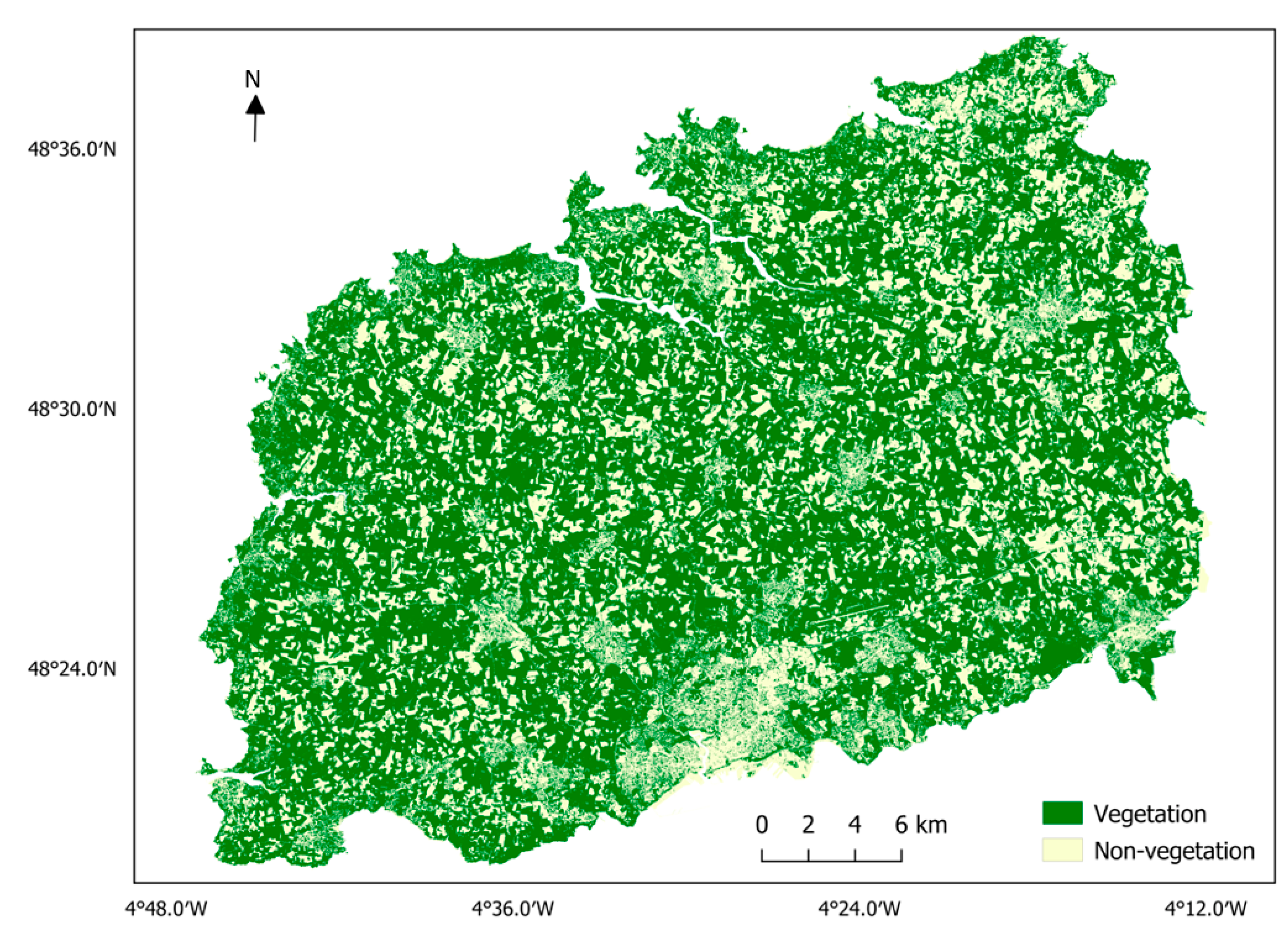
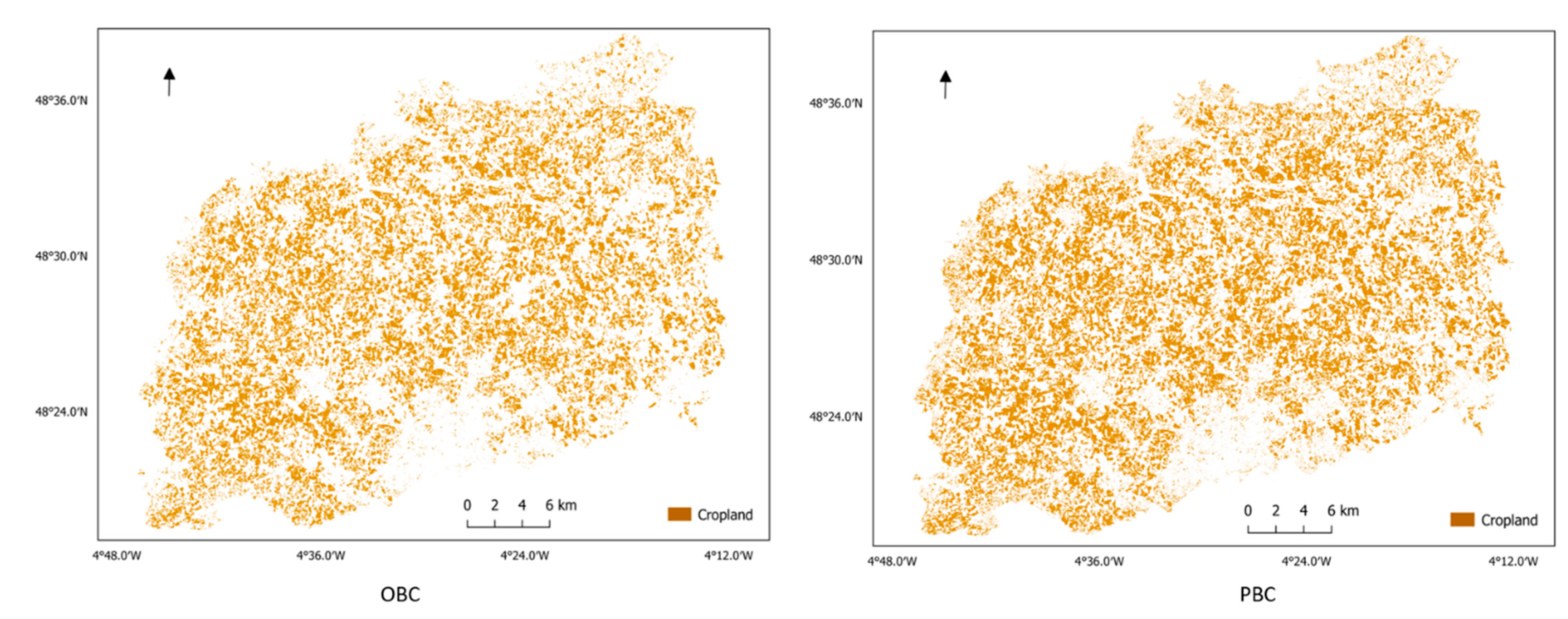
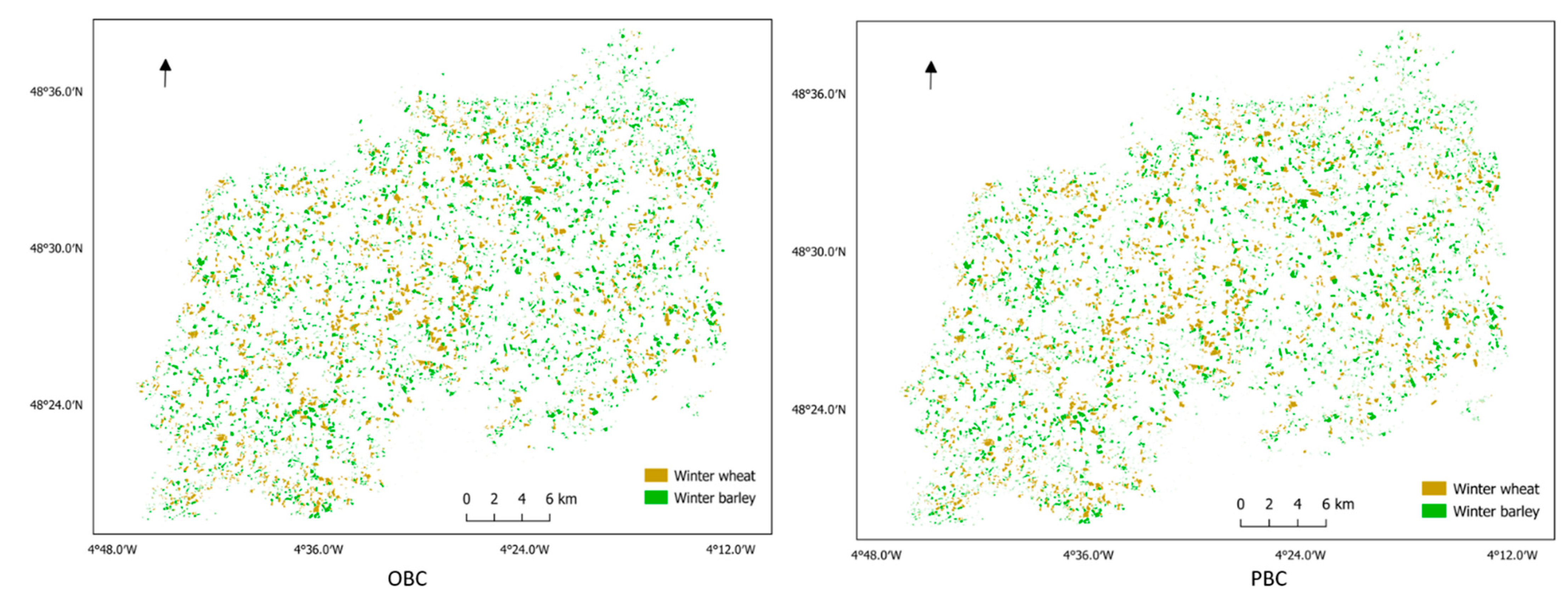
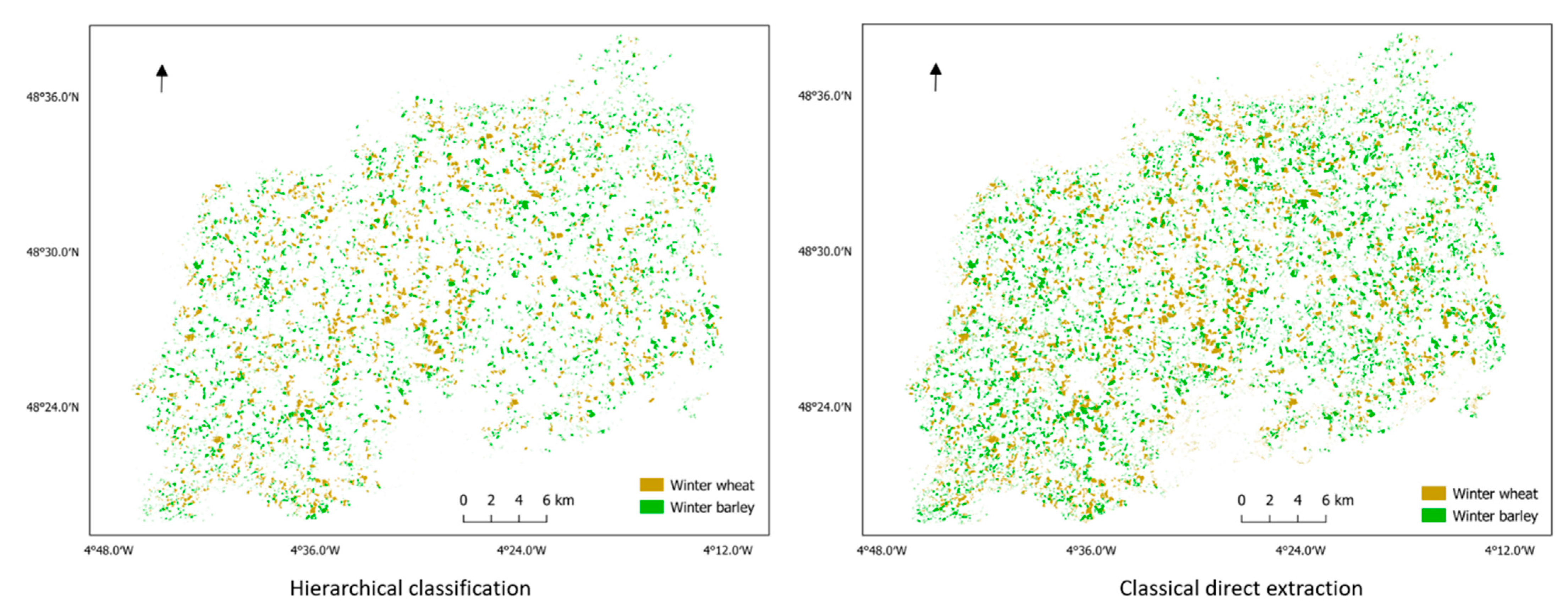
Three issues surrounding winter crops have been studied and discussed in this paper. Firstly, two types of winter crops (winter wheat and winter barley) were mapped by using a Sentinel-2 high-resolution image, and two different classification approaches were performed. Both the hierarchical classification, which turns a complex classification problem into a series of smaller classifications, and the classical direct extraction, which extracts the winter crops directly from the original satellite image, were carried out. The hierarchical classification was composed of three smaller classifications: vegetation extraction from the original image, cropland extraction from the vegetation, and finally the winter crop extraction from other crops. Additionally, PBC and OBC were both performed in the last two steps and evaluated in order to keep the most accurate classification for further processing and analysis. Subsequently, crop phenology monitoring was performed, based on the results of the previous step by using Sentinel-1 C-band SAR time series data, and the three important phenological stages (germination, heading, and ripening (harvesting)) and the main growing periods were identified as well.

To respond to the objectives of the study and as the contribution of this paper, our results showed that winter crops in a fragmented landscape with heterogeneous land cover were successfully detected with high accuracy by using a Sentinel-2 image and the classification approaches that have been proposed. In particular, the hierarchical classification framework significantly improved the classification accuracy (0.1 and 0.06 increase in the kappa and OA, respectively, against classical direct extraction), moreover the classification of winter barley is also enhanced by reducing the confusion between winter barley and grassland with the hierarchical classification framework (0.094 increase in the F-score). Within the hierarchical classification, each classification method has its advantage; OBC slightly outperformed PBC in cropland extraction, yet PBC achieved higher accuracy in winter crops mapping. Although some small differences can be noticed, however there is no significant statistical divergence between the two classification methods.

The results also lead to the conclusion that Sentinel-1 C-band SAR-polarized backscatter time series has great potential to monitor winter agriculture phenology in a coastal area with frequent rainfall. Three phenological stages and main growing periods could be easily identified from the time series in a single polarization or from the ratio, and furthermore the timing of the stages and the growing periods of the crops that are observed in the results highly conform to the field knowledge.

Although very satisfactory results were acquired in this study, some recommendations can be made for further studies, such as applying Sentinel-2 time series or SAR data for crop mapping in order to increase the classification accuracy, and in particular to reduce the confusion between winter barley and grasslands or other crop types. Exploring the potential of the combination of SAR and optical data for identifying more phenological stages and growth periods from the time series is advocated by us.

References

1. Schlund, M.; Erasmi, S. Sentinel-1 Time Series Data for Monitoring the Phenology of Winter Wheat. Remote Sens. Environ. 2020, 246, 111814. [Google Scholar] [CrossRef]
2. Yin, H.; Prishchepov, A.V.; Kuemmerle, T.; Bleyhl, B.; Buchner, J.; Radeloff, V.C. Mapping Agricultural Land Abandonment from Spatial and Temporal Segmentation of Landsat Time Series. Remote Sens. Environ. 2018, 210, 12–24. [Google Scholar] [CrossRef]
3. Song, X.-P.; Potapov, P.V.; Krylov, A.; King, L.; Di Bella, C.M.; Hudson, A.; Khan, A.; Adusei, B.; Stehman, S.V.; Hansen, M.C. National-Scale Soybean Mapping and Area Estimation in the United States Using Medium Resolution Satellite Imagery and Field Survey. Remote Sens. Environ. 2017, 190, 383–395. [Google Scholar] [CrossRef]
4. Sun, C.; Bian, Y.; Zhou, T.; Pan, J. Using of Multi-Source and Multi-Temporal Remote Sensing Data Improves Crop-Type Mapping in the Subtropical Agriculture Region. Sensors 2019, 19, 2401. [Google Scholar] [CrossRef]
5. Birrell, S.J.; Sudduth, K.A.; Borgelt, S.C. Comparison of Sensors and Techniques for Crop Yield Mapping. Comput. Electron. Agric. 1996, 14, 215–233. [Google Scholar] [CrossRef]
6. Song, Y.; Wang, J. Mapping Winter Wheat Planting Area and Monitoring Its Phenology Using Sentinel-1 Backscatter Time Series. Remote Sens. 2019, 11, 449. [Google Scholar] [CrossRef]
7. Arvor, D.; Jonathan, M.; Meirelles, M.S.P.; Dubreuil, V.; Durieux, L. Classification of MODIS EVI Time Series for Crop Mapping in the State of Mato Grosso, Brazil. Int. J. Remote Sens. 2011, 32, 7847–7871. [Google Scholar] [CrossRef]
8. Forkuor, G.; Conrad, C.; Thiel, M.; Ullmann, T.; Zoungrana, E. Integration of Optical and Synthetic Aperture Radar Imagery for Improving Crop Mapping in Northwestern Benin, West Africa. Remote Sens. 2014, 6, 6472–6499. [Google Scholar] [CrossRef]
9. Xie, G.; Niculescu, S. Remote Sensing Mapping and Monitoring of Land Cover/Land Use (LCLU) Changes in the Crozon Peninsula (Brittany, France) from 2007 to 2018 by Machine Learning Algorithms (Support Vector Machine, Random Forest, and Convolutional Neural Network) and by Post-Classification Comparison (PCC). Remote Sens. 2021, 13, 3899. [Google Scholar] [CrossRef]
10. Dong, Q.; Chen, X.; Chen, J.; Zhang, C.; Liu, L.; Cao, X.; Zang, Y.; Zhu, X.; Cui, X. Mapping Winter Wheat in North China Using Sentinel 2A/B Data: A Method Based on Phenology-Time Weighted Dynamic Time Warping. Remote Sens. 2020, 12, 1274. [Google Scholar] [CrossRef] [Green Version]
11. Zhou, T.; Pan, J.; Zhang, P.; Wei, S.; Han, T. Mapping Winter Wheat with Multi-Temporal SAR and Optical Images in an Urban Agricultural Region. Sensors 2017, 17, 1210. [Google Scholar] [CrossRef] [PubMed]
12. Wardlow, B.D.; Egbert, S.L. Large-Area Crop Mapping Using Time-Series MODIS 250 m NDVI Data: An Assessment for the U.S. Central Great Plains. Remote Sens. Environ. 2008, 112, 1096–1116. [Google Scholar] [CrossRef]
13. Jiang, Y.; Lu, Z.; Li, S.; Lei, Y.; Chu, Q.; Yin, X.; Chen, F. Large-Scale and High-Resolution Crop Mapping in China Using Sentinel-2 Satellite Imagery. Agriculture 2020, 10, 433. [Google Scholar] [CrossRef]
14. Del Frate, F.; Ferrazzoli, P.; Guerriero, L.; Strozzi, T.; Wegmuller, U.; Cookmartin, G.; Quegan, S. Wheat Cycle Monitoring Using Radar Data and a Neural Network Trained by a Model. IEEE Trans. Geosci. Remote Sens. 2004, 42, 35–44. [Google Scholar] [CrossRef]
15. Ibrahim, E.S.; Rufin, P.; Nill, L.; Kamali, B.; Nendel, C.; Hostert, P. Mapping Crop Types and Cropping Systems in Nigeria with Sentinel-2 Imagery. Remote Sens. 2021, 13, 3523. [Google Scholar] [CrossRef]
16. Ok, A.O.; Akar, O.; Gungor, O. Evaluation of Random Forest Method for Agricultural Crop Classification. Eur. J. Remote Sens. 2012, 45, 421–432. [Google Scholar] [CrossRef]
17. Tatsumi, K.; Yamashiki, Y.; Canales Torres, M.A.; Taipe, C.L.R. Crop Classification of Upland Fields Using Random Forest of Time-Series Landsat 7 ETM+ Data. Comput. Electron. Agric. 2015, 115, 171–179. [Google Scholar] [CrossRef]
18. Son, N.-T.; Chen, C.-F.; Chen, C.-R.; Minh, V.-Q. Assessment of Sentinel-1A Data for Rice Crop Classification Using Random Forests and Support Vector Machines. Geocarto Int. 2018, 33, 587–601. [Google Scholar] [CrossRef]
19. Rodriguez-Galiano, V.F.; Ghimire, B.; Rogan, J.; Chica-Olmo, M.; Rigol-Sanchez, J.P. An Assessment of the Effectiveness of a Random Forest Classifier for Land-Cover Classification. ISPRS J. Photogramm. Remote Sens. 2012, 67, 93–104. [Google Scholar] [CrossRef]
20. Hao, P.; Zhan, Y.; Wang, L.; Niu, Z.; Shakir, M. Feature Selection of Time Series MODIS Data for Early Crop Classification Using Random Forest: A Case Study in Kansas, USA. Remote Sens. 2015, 7, 5347–5369. [Google Scholar] [CrossRef] [Green Version]
21. Li, H.; Zhang, C.; Zhang, S.; Atkinson, P.M. Crop Classification from Full-Year Fully-Polarimetric L-Band UAVSAR Time-Series Using the Random Forest Algorithm. Int. J. Appl. Earth Obs. Geoinf. 2020, 87, 102032. [Google Scholar] [CrossRef]
22. Saini, R.; Ghosh, S.K. Crop classification on single date sentinel-2 imagery using random forest and suppor vector machine. Int. Arch. Photogramm. Remote Sens. Spatial Inf. Sci. 2018, XLII-5, 683–688. [Google Scholar] [CrossRef]
23. Whiteside, T.G.; Boggs, G.S.; Maier, S.W. Comparing Object-Based and Pixel-Based Classifications for Mapping Savannas. Int. J. Appl. Earth Obs. Geoinf. 2011, 13, 884–893. [Google Scholar] [CrossRef]
24. Weih, R.; Riggan, N. Object-Based Classification vs. Pixel-Based Classification: Comparitive Importance of Multi-Resolution Imagery. Int. Arch. Photogramm. Remote Sens. Spat. Inf. Sci. ISPRS Arch. 2010, 38, C7. [Google Scholar]
25. Nasrallah, A.; Baghdadi, N.; El Hajj, M.; Darwish, T.; Belhouchette, H.; Faour, G.; Darwich, S.; Mhawej, M. Sentinel-1 Data for Winter Wheat Phenology Monitoring and Mapping. Remote Sens. 2019, 11, 2228. [Google Scholar] [CrossRef]
26. Pan, Z.; Huang, J.; Zhou, Q.; Wang, L.; Cheng, Y.; Zhang, H.; Blackburn, G.A.; Yan, J.; Liu, J. Mapping Crop Phenology Using NDVI Time-Series Derived from HJ-1 A/B Data. Int. J. Appl. Earth Obs. Geoinf. 2015, 34, 188–197. [Google Scholar] [CrossRef]
27. Gan, L.; Cao, X.; Chen, X.; Dong, Q.; Cui, X.; Chen, J. Comparison of MODIS-Based Vegetation Indices and Methods for Winter Wheat Green-up Date Detection in Huanghuai Region of China. Agric. For. Meteorol. 2020, 288–289, 108019. [Google Scholar] [CrossRef]
28. Meroni, M.; d’Andrimont, R.; Vrieling, A.; Fasbender, D.; Lemoine, G.; Rembold, F.; Seguini, L.; Verhegghen, A. Comparing Land Surface Phenology of Major European Crops as Derived from SAR and Multispectral Data of Sentinel-1 and -2. Remote Sens. Environ. 2021, 253, 112232. [Google Scholar] [CrossRef]
29. Wali, E.; Tasumi, M.; Moriyama, M. Combination of Linear Regression Lines to Understand the Response of Sentinel-1 Dual Polarization SAR Data with Crop Phenology—Case Study in Miyazaki, Japan. Remote Sens. 2020, 12, 189. [Google Scholar] [CrossRef]
30. Canisius, F.; Shang, J.; Liu, J.; Huang, X.; Ma, B.; Jiao, X.; Geng, X.; Kovacs, J.M.; Walters, D. Tracking Crop Phenological Development Using Multi-Temporal Polarimetric Radarsat-2 Data. Remote Sens. Environ. 2018, 210, 508–518. [Google Scholar] [CrossRef]
31. Mandal, D.; Kumar, V.; Ratha, D.; Dey, S.; Bhattacharya, A.; Lopez-Sanchez, J.M.; McNairn, H.; Rao, Y.S. Dual Polarimetric Radar Vegetation Index for Crop Growth Monitoring Using Sentinel-1 SAR Data. Remote Sens. Environ. 2020, 247, 111954. [Google Scholar] [CrossRef]
32. Géoportail. Available online: https://www.geoportail.gouv.fr/ (accessed on 21 August 2022).
33. Rouault, S. Observer L’occupation des Sols Pour Guider les Politiques D’aménagement (MOS). Available online: https://www.adeupa-brest.fr/nos-publications/observer-loccupation-des-sols-pour-guider-les-politiques-damenagement-mos-0 (accessed on 21 August 2022).
34. Agence d’Urbanisme Brest Bretagne|ADEUPa Brest. Available online: https://adeupa-brest.fr/ (accessed on 21 August 2022).
35. Chambres d’Agriculture de Bretagne. Available online: http://www.chambres-agriculture-bretagne.fr/synagri/accueilRegion (accessed on 22 August 2022).
36. Sentinel-2—Missions—Sentinel Online—Sentinel Online. Available online: https://sentinel.esa.int/web/sentinel/missions/sentinel-2 (accessed on 18 August 2022).
37. Sentinel-1—Missions—Sentinel Online—Sentinel Online. Available online: https://sentinels.copernicus.eu/web/sentinel/missions/sentinel-1 (accessed on 18 August 2022).
38. Registre Parcellaire Graphique (RPG). Available online: https://artificialisation.developpement-durable.gouv.fr/bases-donnees/registre-parcellaire-graphique (accessed on 18 August 2022).
39. Xue, J.; Su, B. Significant Remote Sensing Vegetation Indices: A Review of Developments and Applications. J. Sens. 2017, 2017, 1–17. [Google Scholar] [CrossRef]
40. Bannari, A.; Morin, D.; Bonn, F.; Huete, A.R. A Review of Vegetation Indices. Remote Sens. Rev. 1995, 13, 95–120. [Google Scholar] [CrossRef]
41. Campbell, J.B.; Wynne, R.H. Introduction to Remote Sensing, 5th ed.; Guilford Press: New York, NY, USA, 2011; ISBN 978-1-60918-177-2. [Google Scholar]
42. Rouse, J.W.; Haas, R.H.; Scheel, J.A.; Deering, D.W. Monitoring Vegetation Systems in the Great Plains with ERTS. In Proceedings of the 3rd Earth Resource Technology Satellite (ERTS) Symposium, Washington, DC, USA, 10–14 December 1973; Volume 1, pp. 48–62. [Google Scholar]
43. Gao, B. NDWI—A Normalized Difference Water Index for Remote Sensing of Vegetation Liquid Water from Space. Remote Sens. Environ. 1996, 58, 257–266. [Google Scholar] [CrossRef]
44. Mulianga, B.; Bégué, A.; Clouvel, P.; Todoroff, P. Mapping Cropping Practices of a Sugarcane-Based Cropping System in Kenya Using Remote Sensing. Remote Sens. 2015, 7, 14428–14444. [Google Scholar] [CrossRef]
45. Valero, S.; Arnaud, L.; Planells, M.; Ceschia, E. Synergy of Sentinel-1 and Sentinel-2 Imagery for Early Seasonal Agricultural Crop Mapping. Remote Sens. 2021, 13, 4891. [Google Scholar] [CrossRef]
46. Yin, L.; You, N.; Zhang, G.; Huang, J.; Dong, J. Optimizing Feature Selection of Individual Crop Types for Improved Crop Mapping. Remote Sens. 2020, 12, 162. [Google Scholar] [CrossRef]
47. Gitelson, A.A.; Kaufman, Y.J.; Merzlyak, M.N. Use of a Green Channel in Remote Sensing of Global Vegetation from EOS-MODIS. Remote Sens. Environ. 1996, 58, 289–298. [Google Scholar] [CrossRef]
48. Matsushita, B.; Yang, W.; Chen, J.; Onda, Y.; Qiu, G. Sensitivity of the Enhanced Vegetation Index (EVI) and Normalized Difference Vegetation Index (NDVI) to Topographic Effects: A Case Study in High-Density Cypress Forest. Sensors 2007, 7, 2636–2651. [Google Scholar] [CrossRef]
49. Huete, A.; Didan, K.; Miura, T.; Rodriguez, E.P.; Gao, X.; Ferreira, L.G. Overview of the Radiometric and Biophysical Performance of the MODIS Vegetation Indices. Remote Sens. Environ. 2002, 83, 195–213. [Google Scholar] [CrossRef]
50. Huete, A.R. A Soil-Adjusted Vegetation Index (SAVI). Remote Sens. Environ. 1988, 25, 295–309. [Google Scholar] [CrossRef]
51. Palchoudhuri, Y.; Valcarce-Diñeiro, R.; King, P.; Sanabria-Soto, M. Classification of Multi-Temporal Spectral Indices for Crop Type Mapping: A Case Study in Coalville, UK. J. Agric. Sci. 2018, 156, 24–36. [Google Scholar] [CrossRef]
52. Qi, J.; Chehbouni, A.; Huete, A.R.; Kerr, Y.H.; Sorooshian, S. A Modified Soil Adjusted Vegetation Index. Remote Sens. Environ. 1994, 48, 119–126. [Google Scholar] [CrossRef]
53. Samasse, K.; Hanan, N.P.; Anchang, J.Y.; Diallo, Y. A High-Resolution Cropland Map for the West African Sahel Based on High-Density Training Data, Google Earth Engine, and Locally Optimized Machine Learning. Remote Sens. 2020, 12, 1436. [Google Scholar] [CrossRef]
54. Wyawahare, M.; Kulkarni, P.; Kulkarni, A.; Lad, A.; Majji, J.; Mehta, A. Agricultural Field Analysis Using Satellite Surface Reflectance Data and Machine Learning Technique. In International Conference on Advances in Computing and Data Sciences; Singh, M., Gupta, P.K., Tyagi, V., Flusser, J., Ören, T., Valentino, G., Eds.; Springer: Singapore, 2020; pp. 439–448. [Google Scholar]
55. Li, Z.; Chen, Z. Remote Sensing Indicators for Crop Growth Monitoring at Different Scales. In Proceedings of the 2011 IEEE International Geoscience and Remote Sensing Symposium, Vancouver, BC, Canada, 24–29 July 2011; pp. 4062–4065. [Google Scholar]
56. Witharana, C.; Civco, D.L. Optimizing Multi-Resolution Segmentation Scale Using Empirical Methods: Exploring the Sensitivity of the Supervised Discrepancy Measure Euclidean Distance 2 (ED2). ISPRS J. Photogramm. Remote Sens. 2014, 87, 108–121. [Google Scholar] [CrossRef]
57. Darwish, A.; Leukert, K.; Reinhardt, W. Image Segmentation for the Purpose of Object-Based Classification. In Proceedings of the 2003 IEEE International Geoscience and Remote Sensing Symposium, Toulouse, France, 21–25 July 2003; Volume 3, pp. 2039–2041. [Google Scholar]
58. Benz, U.C.; Hofmann, P.; Willhauck, G.; Lingenfelder, I.; Heynen, M. Multi-Resolution, Object-Oriented Fuzzy Analysis of Remote Sensing Data for GIS-Ready Information. ISPRS J. Photogramm. Remote Sens. 2004, 58, 239–258. [Google Scholar] [CrossRef]
59. ECognition Suite Documentation. Available online: https://docs.ecognition.com/v9.5.0/Page%20collection/eCognition%20Suite%20Documentation.htm?tocpath=Documentation%20eCognition%20Suite%7C_____0 (accessed on 14 April 2021).
60. Richards, J.A.; Jia, X. Supervised Classification Techniques. In Remote Sensing Digital Image Analysis: An Introduction; Richards, J.A., Jia, X., Eds.; Springer: Berlin/Heidelberg, Germany, 1999; pp. 181–222. ISBN 978-3-662-03978-6. [Google Scholar]
61. Gislason, P.O.; Benediktsson, J.A.; Sveinsson, J.R. Random Forests for Land Cover Classification. Pattern Recognit. Lett. 2006, 27, 294–300. [Google Scholar] [CrossRef]
62. Foody, G.M. Status of Land Cover Classification Accuracy Assessment. Remote Sens. Environ. 2002, 80, 185–201. [Google Scholar] [CrossRef]
63. Alberg, A.J.; Park, J.W.; Hager, B.W.; Brock, M.V.; Diener-West, M. The Use of “Overall Accuracy” to Evaluate the Validity of Screening or Diagnostic Tests. J. Gen. Intern. Med. 2004, 19, 460–465. [Google Scholar] [CrossRef]
64. Foody, G.M. Explaining the Unsuitability of the Kappa Coefficient in the Assessment and Comparison of the Accuracy of Thematic Maps Obtained by Image Classification. Remote Sens. Environ. 2020, 239, 111630. [Google Scholar] [CrossRef]
65. Fitzgerald, R.W.; Lees, B.G. Assessing the Classification Accuracy of Multisource Remote Sensing Data. Remote Sens. Environ. 1994, 47, 362–368. [Google Scholar] [CrossRef]
66. Gorelick, N.; Hancher, M.; Dixon, M.; Ilyushchenko, S.; Thau, D.; Moore, R. Google Earth Engine: Planetary-Scale Geospatial Analysis for Everyone. Remote Sens. Environ. 2017, 202, 18–27. [Google Scholar] [CrossRef]
67. Mutanga, O.; Kumar, L. Google Earth Engine Applications. Remote Sens. 2019, 11, 591. [Google Scholar] [CrossRef]
68. Sentinel-1 Algorithms|Google Earth Engine. Available online: https://developers.google.com/earth-engine/guides/sentinel1 (accessed on 4 July 2022).
69. Picard, G.; Le Toan, T.; Mattia, F. Understanding C-Band Radar Backscatter from Wheat Canopy Using a Multiple-Scattering Coherent Model. IEEE Trans. Geosci. Remote Sens. 2003, 41, 1583–1591. [Google Scholar] [CrossRef]
70. Koller, D.; Sahami, M. Hierarchically Classifying Documents Using Very Few Words. In Proceedings of the 14th International Conference on Machine Learning (ICML), San Francisco, CA, USA, 28 June–1 July 2001; Volume 223. [Google Scholar]
71. Costa, E.P.; Lorena, A.C.; Carvalho, A.C.P.L.F.; Freitas, A.A. A Review of Performance Evaluation Measures for Hierarchical Classifiers. In Evaluation Methods for Machine Learning II: Papers from the AAAI-2007 Workshop, AAAI Technical Report WS-07-05; Drummond, C., Elazmeh, W., Japkowicz, N., Macskassy, S.A., Eds.; AAAI Press: Palo Alto, CA, USA, 2007; pp. 1–6. ISBN 978-1-57735-332-4. [Google Scholar]
72. Costa, E.P.; Lorena, A.C.; Carvalho, A.C.P.L.F.; Freitas, A.A.; Holden, N. Comparing Several Approaches for Hierarchical Classification of Proteins with Decision Trees. In Proceedings of the Advances in Bioinformatics and Computational Biology, Angra dos Reis, Brazil, 29–31 August 2007; Sagot, M.-F., Walter, M.E.M.T., Eds.; Springer: Berlin/Heidelberg, Germany, 2007; pp. 126–137. [Google Scholar]
73. Silla, C.N.; Freitas, A.A. A Survey of Hierarchical Classification across Different Application Domains. Data Min. Knowl. Disc. 2011, 22, 31–72. [Google Scholar] [CrossRef]
74. Burred, J.J.; Lerch, A. A Hierarchical Approach to Automatic Musical Genre Classification. In Proceedings of the 6th international Conference on Digital Audio Effects, London, UK, 8–11 September 2003; pp. 8–11. [Google Scholar]
75. Guo, Y.; Liu, Y.; Bakker, E.M.; Guo, Y.; Lew, M.S. CNN-RNN: A Large-Scale Hierarchical Image Classification Framework. Multimed Tools Appl. 2018, 77, 10251–10271. [Google Scholar] [CrossRef]
76. Fan, J.; Gao, Y.; Luo, H. Hierarchical Classification for Automatic Image Annotation. In Proceedings of the 30th Annual International ACM SIGIR Conference on Research and Development in Information Retrieval, Amsterdam, The Netherlands, 23–27 July 2007; Association for Computing Machinery: New York, NY, USA, 2007; pp. 111–118. [Google Scholar]
77. Uca Avci, Z.D.; Karaman, M.; Ozelkan, E.; Kumral, M.; Budakoglu, M. OBIA Based Hierarchical Image Classification for Industrial Lake Water. Sci. Total Environ. 2014, 487, 565–573. [Google Scholar] [CrossRef]
78. Gerylo, G.; Hall, R.J.; Franklin, S.E.; Roberts, A.; Milton, E.J. Hierarchical Image Classification and Extraction of Forest Species Composition and Crown Closure from Airborne Multispectral Images. Can. J. Remote Sens. 1998, 24, 219–232. [Google Scholar] [CrossRef]
79. Liu, D.; Xia, F. Assessing Object-Based Classification: Advantages and Limitations. Remote Sens. Lett. 2010, 1, 187–194. [Google Scholar] [CrossRef]
80. Estoque, R.C.; Murayama, Y.; Akiyama, C.M. Pixel-Based and Object-Based Classifications Using High- and Medium-Spatial-Resolution Imageries in the Urban and Suburban Landscapes. Geocarto Int. 2015, 30, 1113–1129. [Google Scholar] [CrossRef]
81. Fu, B.; Wang, Y.; Campbell, A.; Li, Y.; Zhang, B.; Yin, S.; Xing, Z.; Jin, X. Comparison of Object-Based and Pixel-Based Random Forest Algorithm for Wetland Vegetation Mapping Using High Spatial Resolution GF-1 and SAR Data. Ecol. Indic. 2017, 73, 105–117. [Google Scholar] [CrossRef]
82. Blaschke, T. Object Based Image Analysis for Remote Sensing. ISPRS J. Photogramm. Remote Sens. 2010, 65, 2–16. [Google Scholar] [CrossRef]
83. Castillejo-González, I.L.; López-Granados, F.; García-Ferrer, A.; Peña-Barragán, J.M.; Jurado-Expósito, M.; de la Orden, M.S.; González-Audicana, M. Object- and Pixel-Based Analysis for Mapping Crops and Their Agro-Environmental Associated Measures Using QuickBird Imagery. Comput. Electron. Agric. 2009, 68, 207–215. [Google Scholar] [CrossRef]
84. Belgiu, M.; Csillik, O. Sentinel-2 Cropland Mapping Using Pixel-Based and Object-Based Time-Weighted Dynamic Time Warping Analysis. Remote Sens. Environ. 2018, 204, 509–523. [Google Scholar] [CrossRef]
85. Devadas, R.; Denham, R.J.; Pringle, M. Support vector machine classification of object-based data for crop mapping, using multi-temporal landsat imagery. Int. Arch. Photogramm. Remote Sens. Spat. Inf. Sci. 2012, XXXIX-B7, 185–190. [Google Scholar] [CrossRef]
86. Möller, M.; Lymburner, L.; Volk, M. The Comparison Index: A Tool for Assessing the Accuracy of Image Segmentation. Int. J. Appl. Earth Obs. Geoinf. 2007, 9, 311–321. [Google Scholar] [CrossRef]
87. Kampouraki, M.; Wood, G.A.; Brewer, T.R. Opportunities and Limitations of Object Based Image Analysis for Detecting Urban Impervious and Vegetated Surfaces Using True-Colour Aerial Photography. In Object-Based Image Analysis: Spatial Concepts for Knowledge-Driven Remote Sensing Applications; Lecture Notes in Geoinformation and Cartography; Blaschke, T., Lang, S., Hay, G.J., Eds.; Springer: Berlin/Heidelberg, Germany, 2008; pp. 555–569. ISBN 978-3-540-77058-9. [Google Scholar]
88. Duro, D.C.; Franklin, S.E.; Dubé, M.G. A Comparison of Pixel-Based and Object-Based Image Analysis with Selected Machine Learning Algorithms for the Classification of Agricultural Landscapes Using SPOT-5 HRG Imagery. Remote Sens. Environ. 2012, 118, 259–272. [Google Scholar] [CrossRef]
89. Gao, Y.; Mas, J. A Comparison of the Performance of Pixel Based and Object Based Classifications over Images with Various Spatial Resolutions. Online J. Earth Sci. 2008, 2, 27–35. [Google Scholar]
90. Berhane, T.M.; Lane, C.R.; Wu, Q.; Anenkhonov, O.A.; Chepinoga, V.V.; Autrey, B.C.; Liu, H. Comparing Pixel- and Object-Based Approaches in Effectively Classifying Wetland-Dominated Landscapes. Remote Sens. 2018, 10, 46. [Google Scholar] [CrossRef]
91. Bolton, D.K.; Friedl, M.A. Forecasting Crop Yield Using Remotely Sensed Vegetation Indices and Crop Phenology Metrics. Agric. For. Meteorol. 2013, 173, 74–84. [Google Scholar] [CrossRef]
92. Gao, F.; Zhang, X. Mapping Crop Phenology in Near Real-Time Using Satellite Remote Sensing: Challenges and Opportunities. J. Remote Sens. 2021, 2021, 1–14. [Google Scholar] [CrossRef]
93. Boschetti, M.; Stroppiana, D.; Brivio, P.A.; Bocchi, S. Multi-Year Monitoring of Rice Crop Phenology through Time Series Analysis of MODIS Images. Int. J. Remote Sens. 2009, 30, 4643–4662. [Google Scholar] [CrossRef]
94. De Castro, A.I.; Six, J.; Plant, R.E.; Peña, J.M. Mapping Crop Calendar Events and Phenology-Related Metrics at the Parcel Level by Object-Based Image Analysis (OBIA) of MODIS-NDVI Time-Series: A Case Study in Central California. Remote Sens. 2018, 10, 1745. [Google Scholar] [CrossRef]
95. De Bernardis, C.; Vicente-Guijalba, F.; Martinez-Marin, T.; Lopez-Sanchez, J.M. Contribution to Real-Time Estimation of Crop Phenological States in a Dynamical Framework Based on NDVI Time Series: Data Fusion with SAR and Temperature. IEEE J. Sel. Top. Appl. Earth Obs. Remote Sens. 2016, 9, 3512–3523. [Google Scholar] [CrossRef]
96. Sakamoto, T.; Yokozawa, M.; Toritani, H.; Shibayama, M.; Ishitsuka, N.; Ohno, H. A Crop Phenology Detection Method Using Time-Series MODIS Data. Remote Sens. Environ. 2005, 96, 366–374. [Google Scholar] [CrossRef]
97. Bargiel, D. A New Method for Crop Classification Combining Time Series of Radar Images and Crop Phenology Information. Remote Sens. Environ. 2017, 198, 369–383. [Google Scholar] [CrossRef]
98. Steele-Dunne, S.C.; McNairn, H.; Monsivais-Huertero, A.; Judge, J.; Liu, P.-W.; Papathanassiou, K. Radar Remote Sensing of Agricultural Canopies: A Review. IEEE J. Sel. Top. Appl. Earth Obs. Remote Sens. 2017, 10, 2249–2273. [Google Scholar] [CrossRef]
99. McNairn, H.; Shang, J. A Review of Multitemporal Synthetic Aperture Radar (SAR) for Crop Monitoring. In Multitemporal Remote Sensing: Methods and Applications; Ban, Y., Ed.; Remote Sensing and Digital Image Processing; Springer International Publishing: Cham, Switzerland, 2016; pp. 317–340. ISBN 978-3-319-47037-5. [Google Scholar]
100. Son, N.-T.; Chen, C.-F.; Chen, C.-R.; Toscano, P.; Cheng, Y.-S.; Guo, H.-Y.; Syu, C.-H. A Phenological Object-Based Approach for Rice Crop Classification Using Time-Series Sentinel-1 Synthetic Aperture Radar (SAR) Data in Taiwan. Int. J. Remote Sens. 2021, 42, 2722–2739. [Google Scholar] [CrossRef]
101. Van de Voorde, T.; Vlaeminck, J.; Canters, F. Comparing Different Approaches for Mapping Urban Vegetation Cover from Landsat ETM+ Data: A Case Study on Brussels. Sensors 2008, 8, 3880–3902. [Google Scholar] [CrossRef] [Green Version]
Figure 1. Location of study area, the north of the Finistère department, Brittany, France, as per the RGB band combination of a Sentinel-2 satellite image on 20 April 2019 and the distribution of agricultural land in 2019.
Remotesensing 14 04437 g001
Figure 2. Hierarchical classification methodology used in the study for crop mapping.
Remotesensing 14 04437 g002
Figure 3. Proposed detail image processing methodology chart.
Remotesensing 14 04437 g003
Figure 4. Sentinel-1 image process in the GEE platform.
Remotesensing 14 04437 g004
Figure 5. Level 1: PBC vegetation (including cropland) extraction results.
Remotesensing 14 04437 g005
Figure 6. Level 2: PBC and OBC croplands extraction results.
Remotesensing 14 04437 g006
Figure 7. Level 3: PBC and OBC winter crops extraction results.
Remotesensing 14 04437 g007
Figure 8. Classification results with hierarchical classification and classical direct extraction.
Remotesensing 14 04437 g008
Figure 9. Sentinel-1 temporal backscattering coefficient profiles of different land covers (vegetation, water, urban area, bare soil, winter wheat, and winter barley) in the study area at VV and VH polarizations from 1 October 2018 to 1 September 2019.
Remotesensing 14 04437 g009
Figure 10. Winter wheat and winter barley Sentinel-1 temporal backscattering coefficient profiles at VV, VH, and VH/VV polarizations of the northern part of the Finistère region for the 2018–2019 growing season, with the daily precipitation data and three main phenological stages, which are presented by a vertical line as well.
Remotesensing 14 04437 g010