Forest Height Mapping Using Feature Selection and Machine Learning by Integrating Multi-Source Satellite Data in Baoding City, North China

Abstract

Accurate estimation of forest height is crucial for the estimation of forest aboveground biomass and monitoring of forest resources. Remote sensing technology makes it achievable to produce high-resolution forest height maps in large geographical areas. In this study, we produced a 25 m spatial resolution wall-to-wall forest height map in Baoding city, north China. We evaluated the effects of three factors on forest height estimation utilizing four types of remote sensing data (Sentinel-1, Sentinel-2, ALOS PALSAR-2, and SRTM DEM) with the National Forest Resources Continuous Inventory (NFCI) data, three feature selection methods (stepwise regression analysis (SR), recursive feature elimination (RFE), and Boruta), and six machine learning algorithms (k-nearest neighbor (k-NN), support vector machine regression (SVR), random forest (RF), gradient boosting decision tree (GBDT), extreme gradient boosting (XGBoost), and categorical boosting (CatBoost)). ANOVA was adopted to quantify the effects of three factors, including data source, feature selection method, and modeling algorithm, on forest height estimation. The results showed that all three factors had a significant influence. The combination of multiple sensor data improved the estimation accuracy. Boruta’s overall performance was better than SR and RFE, and XGBoost outperformed the other five machine learning algorithms. The variables selected based on Boruta, including Sentinel-1, Sentinel-2, and topography metrics, combined with the XGBoost algorithm, provided the optimal model (R² = 0.67, RMSE = 2.2 m). Then, we applied the best model to create the forest height map. There were several discrepancies between the generated forest height map and the existing map product, and the values with large differences between the two maps were mostly distributed in the steep areas with high slope values. Overall, we proposed a methodological framework for quantifying the importance of data source, feature selection method, and machine learning algorithm in forest height estimation, and it was proved to be effective in estimating forest height by using freely accessible multi-source data, advanced feature selection method, and machine learning algorithm.

1. Introduction

Forest is an important part of terrestrial ecosystems and plays a vital role in maintaining the global ecological balance, promoting global biological evolution and community succession [1,2,3]. As an important part of the structure parameters of the forest, forest height is not only an essential indicator for the quantitative estimation of forest biomass and terrestrial carbon circulation but also important auxiliary information for evaluating forest resources and establishing earth system models [4,5]. Traditional forest height estimation mainly depends on the means of manual field surveys. Although the ground survey method has high accuracy, it is timing and force-consuming, and it is difficult to achieve large-range and long-span forest height estimation and dynamic change monitoring [6]. The increasingly developed remote sensing technology has the advantages of multi-time phase, multi-scale, multi-sensor, and rapid macro monitoring. It has become an important way to estimate forest height by constructing empirical models combining remote sensing data and ground-measured data [7].

At present, the most recent advancement in remote sensing technology advocates producing forest height maps of large geographical areas with high resolution. Multispectral data [8,9,10], Light Detection and Ranging (LiDAR) [11,12,13,14], Synthetic Aperture Radar (SAR) [15,16], and other remote sensing data [17] were widely applied. LiDAR data are often regarded as the best remote sensing data source for forest structure parameters due to its direct ability to detect forest vertical structures; however, terrestrial laser scanning (TLS) and airborne laser scanning (ALS) are typically limited by high application costs [18], and it is difficult to generate wall-to-wall forest height maps in large areas due to the sparse measurements in the space of satellite LiDAR [19] Compared to lidar data, optical data are more susceptible to the influence of weather conditions and has issues such as limited sensitivity and low saturation in dense vegetation areas, SAR data are susceptible to terrain and speckle noise, and there is a problem of backscatter signal saturation in high vegetation coverage areas as well as optical data. Nevertheless, the backscattering coefficient of SAR and the rich spectral information of the optical data can also reflect the information about the structure and function of the forest [20,21]. Most importantly, optical data and SAR data can be obtained frequently, continuously, and at a low cost from various spaceborne platforms. In the past few years, numerous studies have shown that spectral reflectance, vegetation index, and spatial texture information extracted from Sentinel-2 images, backscattering coefficients, indices, and texture features calculated from Sentinel-1 C-band, ALOS-2 PALSAR-2 L-band images, and topographic metrics were effective in estimating forest canopy height and other forest parameters [22,23,24,25,26].

As mentioned above, there are many potential feature variables when estimating forest height using multi-source remote sensing data. High-dimensional feature variables will increase the computational load, data noise, and interference, and the problem of complex collinearity between variables will cause the redundancy of variables, which will affect the efficiency and accuracy of modeling [27,28]; therefore, the correct and efficient feature selection phase is an essential step for forest height estimation. However, because of the diverse characteristics of the sensor data and the complex biophysical environment in the forestry areas, the different feature selection methods correspond to different data structures and features, what effect of feature selection method on forest height estimation, and how to determine the best feature selection method is still poorly understood [27]. Stepwise regression analysis is the most commonly used variable selection approach in forest parameter investigations and related studies have reported positive outcomes [29,30,31]. In addition, the Boruta and recursive feature elimination are both well-established wrapper methods, which have been widely applied in the study of forestry research in recent years [32,33,34,35]. Several studies have been conducted to examine the impact of different feature selection strategies in predicting forest characteristics [36,37]. Nevertheless, to our knowledge, there is rarely research conducted to examine the impact of feature selection methods for different remote sensing data sources when estimating forest height.

Another key factor of forest height estimation is the regression algorithm. Currently, regression models used to estimate forest height can be divided into two categories: parametric and non-parametric algorithms. In the parametric model, there are quantitative mathematical expressions between the independent and dependent variables, which are intuitive and simple to understand. Multiple linear regression, stepwise regression, and partial least squares regression are common parametric models; however, the parameter model needs to meet the premise that the relationships between dependent and independent variables have clear model structures, while the relationship between forest height and remote sensing factors is typically quite complex, which limits the application of parametric models [27]. Compared with parametric algorithms, non-parametric algorithms based on data mining, machine learning, and other mathematical theory and methods, through the way of data-driven achieving complex nonlinear relationship prediction, are widely used in forest height estimation, including k-nearest neighbor (k-NN), support vector machine regression (SVR) and random forest (RF) [38,39,40,41,42]. Moreover, some decision-tree-based ensemble algorithms, such as gradient boosting decision tree (GBDT), extreme gradient boosting (XGBoost), and categorical boosting (CatBoost), have performed well in the estimation of forest aboveground biomass [43,44]; however, these algorithms are rarely employed to estimate forest height, and their efficacy has yet to be evaluated.

In summary, to address the gaps mentioned above, we proposed a methodological framework for forest height estimation and mapping using multi-source remote sensing data (Sentinel-2, Sentinel-1, ALOS PALSAR-2, SRTM DEM), three feature selection methods (SR, RFE, Boruta) and six machine learning algorithms (k-NN, SVR, RF, GBDT, XGBoost, and CatBoost) in Baoding city, north China. The purposes of this study are as follows:

(1) To examine the influence of feature selection methods of different remote sensing data sources on forest height estimation, and to explore the optimal feature selection method;

(2) To evaluate the performance of machine learning algorithms based on different feature selection methods in forest tree height estimation;

(3) To generate a forest height distribution map of 25 m spatial resolution in Baoding city, and to analyze the important factors in forest height estimation.

2. Materials and Methods

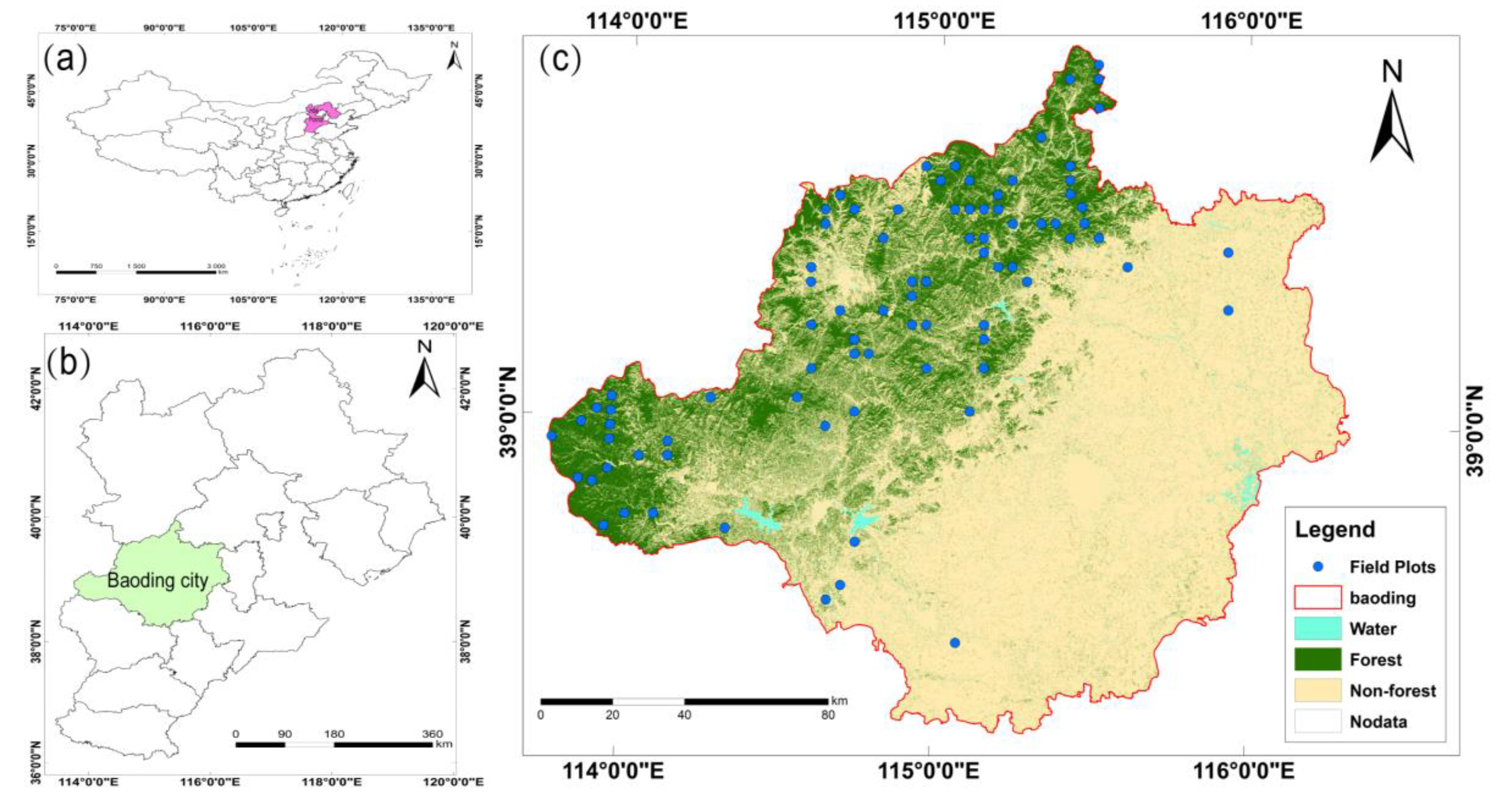
2.1. Study Area

The study area is located in Baoding city in the Midwest of Hebei province, China (38°14–39°57′N, 113°45–116°19′E), covering an area of about 2,211,200 hectares (Figure 1). It is situated near the eastern foot of the northern Taihang Mountains and on the western part of the Jizhong plain. The terrain is inclined from northwest to Southeast. The landforms in the west are mountainous, which are composed of mountains and hills; the landforms in the east region belonging to the North China Plain are flat. Baoding is in the warm temperate continental monsoon climate zone, with an annual average temperature of 12.7 °C and 2511 h of sunshine per year, accounting for 56% of total sunshine hours. The annual frost-free period is about 165–210 days. The period from June to August each year is a period of intensive precipitation, and the average annual precipitation duration is 68 days with an average precipitation of 489.9 mm. The forestry area of Baoding is nearly 590,000 hectares, accounting for approximately 28% of the administrative area of the city, and the forest stock of the whole city reaches 13.7 million cubic meters. Forest types mainly include coniferous forest, broadleaf forest, and mixed conifer-broad-leaf forest. Among them, coniferous trees are mainly Chinese pine (Pinus tabulaeformis) and oriental arborvitae (Platycladus orientalis); Broadleaf trees mainly include populus tremula (Populus davidana), Mongolian oak (Quercus mongolica), white birch (Betula platydiana), and acacia (Robinia pseudoacacia).

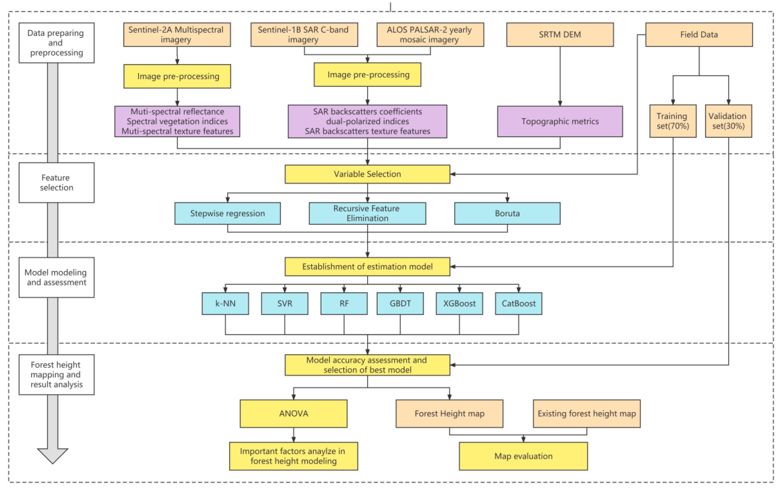
2.2. Methodological Framework of This Study

In this study, we proposed a methodological framework utilizing different feature selection methods and machine learning algorithms to establish forest height estimation models based on multi-source satellite data in the forest regions of Baoding city, north China. Our methodological framework consists of four primary components (Figure 2): (1) data preparation and preprocessing, (2) feature variables selection, (3) model building and assessment, and (4) forest height mapping and important factors analysis.

2.3. Data Source and Preprocessing

2.3.1. Field Data Collection

The field data utilized in this study is the ninth National Forest Resources Continuous Inventory (NFCI) data of Hebei Province. The field survey was conducted in November 2016. The sample plots were systematically arranged at an interval of 4 km × 4 km along a vertical and horizontal coordinate system. The sample plot was a square plot with a side length of 25.82 m, and each sample plot area was about 0.067 ha.

Each tree with a diameter at breast height (DBH) higher than 5 cm had its DBH, tree height, and crown height measured, as well as the land use, dominant tree species, tree species composition, average DBH, and average tree height were recorded. There were 1210 sample plots in Baoding city, and 128 sample plots were finally collected after removing the sample plots of non-forest land and inadequate information. The average tree height of the forest sample plot ranged from 3.00 m to 24.50 m, and the average, median, and standard deviation (std) were 8.57 m, 7.30 m, and 3.89 m, respectively. Among the 128 sample plots, 91 sample plots (70%) were randomly selected for training, and the remaining 37 sample plots (30%) were used as the validation data set for the machine learning model (

Table 1. The statistics of forest height in training, testing, and total sample datasets.

Dataset	Sample Size	Min (m)	Max (m)	Mean (m)	Median (m)	Std (m)
Training	91	3.00	24.50	8.57	7.50	3.92
Validation	37	3.20	18.40	8.58	7.20	3.87
Total	128	3.00	24.50	8.57	7.30	3.89

).

2.3.2. Sentinel-2 Multispectral Imagery and Preprocessing

The multispectral images used in this study were Sentinel-2 satellite images from the European Space Agency (ESA). The multispectral imager instrument carried by the Sentinel-2 satellite has the advantages of high spatial resolution, excellent multispectral imaging capacity, wide wing, and short revisit cycle, which can be used to monitor the distribution and health of forests. The Sentinel-2 satellite image incorporates 13 bands, with spatial resolutions of 10 m for bands 2–4 and 8 (blue: 490 nm, green: 560 nm, red: 665 nm, and NIR: 842 nm), 20 m for bands 5–7, 8A, 11, and 12 ((red edge 1: 705 nm, red edge 2: 740 nm, red edge 3: 783 nm, narrow NIR: 865 nm, SWIR1: 1610 nm, and SWIR2: 2190 nm), and 60 m for the other three bands (coastal aerosol: 443 nm, water vapor: 940 nm, and SWIR cirrus: 1375 nm). The bands with spatial resolutions of 10 m and 20 m were employed in this study.

In order to match the time of sample plot data collection, we downloaded seven Sentinel-2 Level-1C images covering the study area with less than 10% cloud from the United States Geological Service’s Earth Explorer (USGS) (https://earthexplorer.usgs.gov/ (accessed on 24 March 2022)) which were obtained in the growing season in August 2016. Since the Sentinel-2 Level-1C image is the top atmospheric reflectance image, we used the atmospheric correction processor (version 2.5.5, European Space Agency, Paris, France) of Sentinel Application Platform (SNAP) software (version 8.0, ESA, Paris, France) to acquire the Level-2A products, the bottom-of-atmosphere-corrected reflectance images. To match the field plot sizes, we resampled the preprocessed Sentinel-2 images to 25 m pixel sizes. Then, mosaicking and clipping were completed to cover the study area.

2.3.3. Synthetic Aperture Radar (SAR) Data and Preprocessing

We used synthetic aperture radar data from two different data sources, including the Sentinel-1 C-band imagery and ALOS-2 PALSAR-2 yearly mosaic imagery.

Sentinel-1 is composed of two polar-orbiting satellites, and the revisit period of a single satellite is 12 days. A total of 10 sentinel-1 ground range detected (GRD) images with good quality from October 2016 were obtained from the Google earth engine (GEE) cloud computing platform. We acquired the dual-polarization (VV and VH) images in Interferometric Wide swath (IW) mode with an ascending orbital pass. These images in GEE were already processed by the ESA Sentinel-1 toolbox, including thermal noise removal, radiometric correction, terrain correction, and conversion of the backscattering coefficient to decibels [45]. Here, we further processed them according to the framework proposed by Mullissa et al. in 2021 [46], including border noise correction, refined Lee filter for speckle filtering, and radiometric terrain normalization.

Due to the fact that PALSAR- 2 images in Baoding city were not free, the L-band SAR imagery had not been applied for this study; however, the Japan Aerospace Exploration Agency (JAXA) provides the 25 m spatial resolution ALOS/PALSAR yearly mosaic, which is produced by mosaicking SAR images measured by PALSAR-2 available each year [47]. We obtained the mosaic data in the year 2016 from GEE in this study. This SAR imagery was already ortho-rectificatied by using the 90 m SRTM Digital Elevation Model. The data were stored as 16-bit digital numbers (DN), which were converted to gamma naught values (γ₀) in decibel unit (dB) using the following equation: γ₀ = 10log₁₀(DN²) − 83.0 dB. All of the SAR images were resampled to the same pixel sizes to ensure consistency with other data.

2.3.4. Topographic and Ancillary Data

The digital elevation model (DEM) reflects the abundant terrain information of the mountain region and provides great assistance to forest height estimation [23]. In this study, we used the Shuttle Radar Topography Mission (SRTM) V3 product, which was provided by NASA JPL at a resolution of approximately 30 m. Furthermore, we applied the FROM-GLC 2017 (Finer Resolution Observation and Monitoring of Global Land Cover at30-m resolution, 2017v1) product to define the forest regions of the study area [48].

2.4. Feature Variable Extraction

Based on the remote sensing data sources mentioned above, a total of 153 feature variables were extracted in this study (

Table 2. Summary of the metrics extracted from multi-source data used in this study.

Source		Feature Variables	Description
Sentinel-2 multispectral data	Multispectral bands (10)	b2	Blue, 490 nm
		b3	Green, 560 nm
		b4	Red, 665 nm
		b5	Red edge, 705 nm
		b6	Red edge, 749 nm
		b7	Red edge, 783 nm
		b8	Near-infrared, 842 nm
		b8a	Near-infrared, 865 nm
		b11	Short-wave infrared, 1610 nm
		b12	Short-wave infrared, 2190 nm
	Vegetation indices (20)	SAVI	Soil adjusted vegetation index, 1.5 × (B8−B4)/(B8 + B4 + 0.5)
		NDVI	Normalized difference vegetation index, (B8 − B4)/(B8 + B4)
		MSAVI2	Second modified soil adjusted vegetation index, 0.5 × [2 × (B8 + 1) − sqrt[(2 × B8 + 1) × (2 × B8 + 1) – 8 × (B8 − B4)]]
		RVI	Ratio vegetation index, B8/B4
		PVI	Perpendicular vegetation index, sin(a) × B8 − cos(a) × B4(a = 45°)
		IPVI	Infrared percentage vegetation index, B8/(B8 + B4)
		WDVI	Weighted difference vegetation index, B8 − 0.5 × B4
		TNDVI	Transformed normalized difference vegetation index, sqrt[(B8 − B4)/(B8 + B4) + 0.5]
		GNDVI	Green normalized difference vegetation index, (B8 − B3)/(B8 + B3)
		CI	Color index, (B4 − B3)/(B4 + B3)
		ARVI	Atmospherically resistant vegetation index, (B8 – 2 × B4 + B2)/(B8 + 2 × B4 − B2)
		MCARI	Modified chlorophyll absorption ratio index, [(B5 − B4) − 0.2 × B5 − B3)] × (B5 − B4)
		MTCI	Meris terrestrial chlorophyll index, (B6 − B5)/(B5 − B4)
		EVI	Enhanced vegetation index, 2.5 × [(B8 − B4)/(B8 + 6 × B4 − 7.5 × B2 + 1)]
		EVI2	Enhanced vegetation index2, 2.5 × [(B8 − B4)/(B8 + 2.4 × B4 + 1)]
		NDVIre1	Normalized Difference Vegetation Index red-edge1,(B8 − B5)/(B8 + B5)
		NDVIre2	Normalized Difference Vegetation Index red-edge1, (B8cB6)/(B8 + B6)
		mNDVI	Modified normalized difference vegetation index, (B8 − B4)/(B8 + B4 − 2 × B2)
		mNDVIre	Modified red edge normalized difference vegetation index, (B8 − B5)/(B8 + B5 − 2 × B2)
		NDII	normalized difference infrared index, (B8 − B11)/(B8 + B11)
		SAVI	Soil adjusted vegetation index, 1.5 × (B8 − B4/(B8 + B4 + 0.5)
		NDVI	Normalized difference vegetation index, (B8 − B4)/(B8 + B4)
		MSAVI2	Second modified soil adjusted vegetation index, 0.5 × [2 × (B8 + 1) − sqrt[(2 × B8 + 1) × (2 × B8 + 1) − 8 × (B8 − B4)]]
		RVI	Ratio vegetation index, B8/B4
		PVI	Perpendicular vegetation index, sin(a) × B8 − cos(a) × B4, (a = 45°)
		IPVI	Infrared percentage vegetation index, B8/(B8 + B4)
	Texture (80)	b2/b3/b4/b5/b6/b7/b8/b8a/b11/b12_con	Contrast
		b2/b3/b4/b5/b6/b7/b8/b8a/b11/b12_corr	Correlation
		b2/b3/b4/b5/b6/b7/b8/b8a/b11/b12_dis	Dissimilarity
		b2/b3/b4/b5/b6/b7/b8/b8a/b11/b12_ent	Entropy
		b2/b3/b4/b5/b6/b7/b8/b8a/b11/b12_hom	Homogeneity
		b2/b3/b4/b5/b6/b7/b8/b8a/b11/b12_mean	Mean
		b2/b3/b4/b5/b6/b7/b8/b8a/b11/b12_sm	Angular second moment
		b2/b3/b4/b5/b6/b7/b8/b8a/b11/b12_var	Variance
Sentinel-1 and PALSAR-2 mosaic	Polarization (8)	VV	Vertical transmit-vertical channel backscattering coefficients, dB
		VH	Vertical transmit-horizontal channel backscattering coefficients, dB
		HH	Horizontal transmit- horizontal channel backscattering coefficients, dB
		HV	Horizontal transmit-vertical channel backscattering coefficients, dB
		V/H	VV/VH
		s1npdi	(VV − VH)/(VV + VH)
		H/V	HH/HV
		p2npdi	(HH − HV)/(HH + HV)
	Texture (32)	VV/VH/HH/HV_con	Contrast
		VV/VH/HH/HV_corr	Correlation
		VV/VH/HH/HV_dis	Dissimilarity
		VV/VH/HH/HV_ent	Entropy
		VV/VH/HH/HV_hom	Homogeneity
		VV/VH/HH/HV_mean	Mean
		VV/VH/HH/HV_sm	Angular second moment
		VV/VH/HH/HV_var	Variance
SRTM DEM	(3)	elevation	elevation
		slope	slope
		aspect	aspect

). For Sentinel-2 data, we extracted 10 multispectral variables from the average surface reflectance of 10 multispectral bands with spatial resolutions of 10 m and 20 m. Then, 20 vegetation indices derived from Sentinel-2 data, which were widely used in previous forest studies, were calculated [49,50,51]. Moreover, the texture features of 10 multispectral bands, including mean, variance, homogeneity, contrast, dissimilarity, entropy, second moment, and correlation, were calculated by using the gray level co-occurrence matrix (GLCM) with a 3 × 3 window. Finally, a total of 110 feature variables derived from Sentinel-2 data were obtained. As to SAR data, we extracted VH and VV backscattering coefficients from Sentinel-1 imagery and HH and HV backscattering coefficients from ALOS PALSAR-2 yearly mosaic, respectively. After that, the ratio and normalized polarized difference of VH, VV, and HV, HH were calculated as candidate variables, respectively. GLCM was also used to compute the texture features of VH, VV, HH, and HV backscattering coefficients by using a 3 × 3 window. Finally, 40 SAR feature variables were obtained. In addition, we extracted elevation, slope, and aspect from the DEM image as terrain factors. To analyze the impact of different data sources on forest height estimation, five combination scenarios were designed in this study (

Table 3. Different scenarios of feature variable combinations for forest height modeling.

Scenario ID	Variable Combination	Short Name
1	Sentinel-2	s2
2	Sentinel-2, SRTM DEM	s2to
3	Senitnel-1, Sentinel-2, PALSAR-2 mosaic	s1s2p2
4	Sentinel-1, PALSAR-2 mosaic, SRTM DEM	s1p2to
5	Sentinel-1, Sentinel-2, PALSAR-2 mosaic, SRTM DEM	s1s2p2to

).

2.5. Feature Variable Selection

In this study, we employed stepwise regression analysis, recursive feature elimination, and Boruta methods to select and analyze feature variables from five combination scenarios, with all field measurements serving as a reference.

2.5.1. Stepwise Regression Analysis

In the past few decades, stepwise regression analysis (SR) has been widely used for feature selection for forest parameters estimation studies [22,52,53,54]. The basic principle of stepwise regression is to successively add the most contributing predictor variables in order. After adding each new variable, all variables that no longer improve the model fit were removed. The program will stop running until no variables are selected or dropped [31]. In our research, we screened the best subset of variables by iterative both-direction stepwise regression based on the Akaike information criterion (AIC) and ensured the p-values of all the selected variables were significant (p < 0.05) [55]. This procedure was performed in R 4.2.0 using the “MASS” package [56].

2.5.2. Recursive Feature Elimination

Recursive feature elimination (RFE) is a wrapper-based feature-ranking algorithm for determining the best feature subset [57]. It is essentially a process that repeatedly builds a model until an optimal subset of features is selected. Based on the screening results, the features with the smallest coefficients are deleted first, and the procedure is repeated in the remaining set of features until all features are traversed by the algorithm [58]. During the process of selection, the root mean square error and standard deviation error of 10-fold cross-validation were used to determine the feature variable subset. Although many feature selection methods fusing RFE and other algorithms were proposed, previous research emphasized that RFE combined with random forest could provide unbiased and stable results and improve accuracy [59]; therefore, we used the “rfe()” function of the “caret” package in R 4.2.0 to realize the procedure with the method “Repeatedcv”, repeat “10”, and the function “random forests (rfFuncs)”.

2.5.3. Boruta

The Boruta algorithm is a wrapper built around the random forest classification algorithm implemented in the R package “randomForest”. Its core idea is to construct shadow features by shuffling the original real features and aggregate the original features and shadow features as the feature matrix for training, and then, with the feature importance score of shadow features as a reference, the feature set related to the dependent variable is selected from the original real features. The Boruta algorithm consists of the following steps: First, to create the shadow attributes by shuffling the values of the original object feature and splice the shuffled features with the original real features to form a new feature matrix. Next, use the new feature matrix as input and run the random forest classifier and compute the Z scores of the real feature and shadow feature. Thirdly, to find the maximum Z score among shadow attributes (MZSA), features that were significantly greater than MZSA were labeled as “important”, significantly smaller than MSZA as “unimportant”, and were permanently removed from the feature set. Lastly, to repeat the process until all the features were classified as “important" or "unimportant”. This procedure was performed in R 4.2.0 using the Boruta packages [60].

2.6. Machine Learning Algorithms

In this study, we employed k-nearest neighbor (k-NN), support vector machine regression (SVR), random forest (RF), gradient boosting decision tree (GBDT), extreme gradient boosting (XGBoost), and categorical boosting (CatBoost) machine learning algorithms to model with the training data serving as the input.

2.6.1. K-Nearest Neighbor

The k-nearest neighbor (k-NN) algorithm is a simple and efficient non-parametric method, which can effectively avoid the collinearity problem of the independent variables. It applies to remote sensing data parameter estimation with non-normal distribution and unknown density function and is widely used in forestry investigations around the world [61,62]. The core idea of this algorithm is to take a point in the feature space as the reference object, record the attribute values of the k nearest sample points from the point, and calculate the average value of its inverse distance weight to get the predicted value of this object.

2.6.2. Support Vector Machine Regression

The support vector machine algorithm was proposed based on the VC dimension theory and the structural risk minimization principle [63]. It was initially applied for classification in forest applications, and recently also showed reliable advantages in forest parameter retrieving [64,65]. The basic idea of SVR is to map the features of training data to a high-dimensional feature space by defining a kernel function and finding an optimal hyperplane of linear regression in this feature space to fit the eigenvalues. In the case of limited sample information and high dimensions of feature variables, it can minimize the sampling error and has good generalization ability.

2.6.3. Random Forest

Random forest (RF) is a modified ensemble machine learning algorithm based on decision trees proposed in 2001 [66]. Numerous studies have demonstrated that RF can accurately estimate forest metrics [22,67,68,69]. RF constructs a series of regression trees, each of which is generated by randomly repeated sampling bootstrap training samples that can be put back, which makes some data may be used many times, while other data may not be used. Usually, 70% of the training samples are selected as the modeling samples, and the remaining 30% samples are used to evaluate the sample prediction error, which is called out-of-bag error (OOB error). At the same time, it randomly selects variables at the nodes of each tree. The procedure stops running when the trees without pruning grow to the maximum scale, and the final prediction accuracy takes the average weight of all prediction regression trees. Because of its random characteristic, this method can enhance the stability of the model, improve the prediction accuracy, and increase the robustness of the model itself to noise or overfitting phenomena to a certain extent.

2.6.4. Gradient Boosting Decision Tree

Gradient boosting decision tree (GBDT) is an integrated decision tree algorithm based on the iterative ideas of gradient boosting first proposed by Friedman [70]. It first generates a weak learner (usually a CART regression tree model), obtaining the residual of the input after training, and then trains the next learner based on the residual generated by the previous round of learners, iteratively. In the process of each iteration, each learner aims to minimize the loss function, that is, to make the loss function always reduce the residual along the descending direction of the gradient. Finally, the final prediction result is obtained by accumulating the results of all weak learners. GBDT is very robust to outliers due to the use of some robust loss functions, and in the case of relatively little tuning time, the prediction accuracy can also be relatively high. Although GBDT is very popular in the field of machine learning, it is rarely applied in the study of forest parameter estimation [43,71].

2.6.5. Extreme Gradient Boosting

Extreme gradient boosting (XGBoost) is an improved GBDT algorithm proposed by Chen et al. in the Kaggle machine learning competition [72]. Compared with GBDT, XGBoost has the following advantages: (1) Regular terms are added to the objective function to control the complexity of the model and prevent the learned model from overfitting. (2) The second-order Taylor expansion is used for the objective function, which makes the definition of the objective function more accurate and easier to find the optimal solution; (3) XGBoost builds all possible subtrees from top to bottom first and then prunes from bottom to top in reverse. In this way, it is not easy to fall into the local optimal solution. (4) XGBoost supports parallel processing. It sorts the data in advance before training and then saves it as a block structure. This structure is used repeatedly in subsequent iterations, which greatly reduces the amount of calculation. Due to the advantages of XGBoost, such as sparse data processing ability, greatly increasing algorithm speed, and reducing computational memory in large-scale data training, it has recently attracted a lot of attention. There were also some studies using XGBoost to estimate forest parameters and achieved good results [43,73,74,75].

2.6.6. Categorical Boosting

Categorical boosting (CatBoost), as the name suggests, consists of categorical and boosting, which is a novel gradient boosting algorithm implemented with oblivious trees as the base learner proposed by Dorogush et al. [76]. On the one hand, CatBoost builds fully symmetric trees. In each step, the leaves of the previous tree are split using the same conditions. The feature segmentation pair with the lowest loss was selected and used for nodes at all levels. This balanced tree structure facilitates an efficient CPU implementation and reduces the prediction time. On the other hand, CatBoost uses the concept of rank-lifting to train models on a subset of the data while computing the residuals on another subset, thus preventing target leakage and overfitting. Compared with other algorithms in the boosting family, CatBoost can automatically process discrete feature data, which is suitable for regression problems with multiple input features and regression data containing noisy samples. The model has stronger robustness and generalization performance and performs better in algorithm accuracy. Although CatBoost outperformed other machine learning algorithms in other fields [77,78], the effectiveness of this algorithm for forest height estimation remains to be confirmed.

2.6.7. Tuning the Hyperparameters for the Machine Learning Algorithms

When estimating the forest height, the hyperparameters of the machine learning algorithms can greatly affect the results of the model predictions; therefore, the hyperparameters must be optimized for each algorithm before doing any further examination or comparison using these algorithms. In this study, we utilized grid search technology to automatically perform hyperparameter tuning. Six machine algorithms were hyperparameter tuned based on the lowest model RMSE achieved by the 10-fold cross-validation techniques repeated 5 times on the training dataset. This procedure was performed in R 4.2.0 using the “caret” packages. Detailed information about the key tuning hyperparameters and corresponding tuning parameters configurations for each algorithm were presented in

Table 4. Tuning hyperparameters and corresponding configurations for each algorithm.

Algorithm	Hyperparameter	Description	Hyperparameter Configurations
k-NN	k	the number of neighbors considered.	(1–10) at intervals of 1
SVR	C	the cost of constraints violation	(1–10) at intervals of 1
	gamma	the parameter needed for all kernels except linear	(0–0.2) at intervals of 0.01
RF	mtry	the number of predictor variables randomly sampled at each split	(1–10) at intervals of 1
	ntree	the number of trees	(100–1000) at intervals of 100
GBDT	ntree	the number of trees	(100–1000) at intervals of 100
	maxdepth	the depth of the tree	(1–10) at intervals of 1
	shrinkage	the learning rate	(0.01–0.1) at intervals of 0.01
	min terminal node	the minimum samples required in a terminal node.	(1–10) at intervals of 1
XGBoost	max_depth	the depth of the tree	(1–10) at intervals of 1
	eta	the learning rate	(0.01–0.1) at intervals of 0.01
	gamma	minimum loss reduction of the tree	(0–1) at intervals of 0.1
	colsample_bytree	the number of predictor variables supplied to a tree	(0–1) at intervals of 0.1
	min_child_weight	minimum number of instances	(1–10) at intervals of 1
	subsample	the number of observations supplied to a tree	(0–1) at intervals of 0.1
CatBoost	depth	the depth of the tree
	learning_rate	the learning rate	(0.01–0.1) at intervals of 0.01
	l2_leaf_reg	the coefficient at the L2 regularization term of the cost function	(1–10) at intervals of 1
	rsm	the percentage of features to use at each split selection	(0–1) at intervals of 0.1

.

2.7. Model Evaluation

In our research, we randomly divided the plot data into two sets: training dataset (70%) and validation dataset (30%). The training set was used to train and develop the models, while the validation set did not participate in the model-building process and was instead used to evaluate model performance. The best model was developed based on the training set after hyperparameter tuning, and model performance metrics were produced based on the validation set. The determination coefficient (${\mathrm{R}}^2$, Equation (1)), root mean square error (RMSE, Equation (2)), and relative root mean square error (rRMSE, Equation (3)) were employed to evaluate the performance of different models. The higher the ${\mathrm{R}}^2$ is, the lower the RMSE and rRMSE are, which means that the higher the prediction accuracy is, the better the estimation result is.

$${\mathrm{R}}^2=1-\frac{{{\displaystyle \sum }}_{\mathrm{i}=1}^{\mathrm{n}}{\left({\mathrm{y}}_{\mathrm{i}}-{\hat{\mathrm{y}}}_{\mathrm{i}}\right)}^2}{{{\displaystyle \sum }}_{\mathrm{i}=1}^{\mathrm{n}}{\left({\mathrm{y}}_{\mathrm{i}}-\overline{\mathrm{y}}\right)}^2}$$

(1)

$$\mathrm{RMSE}=\sqrt{\frac{{{\displaystyle \sum }}_{\mathrm{i}=1}^{\mathrm{n}}{\left({\mathrm{y}}_{\mathrm{i}}-{\hat{\mathrm{y}}}_{\mathrm{i}}\right)}^2}{\mathrm{n}}}$$

(2)

$$\mathrm{rRMSE}=\frac{\mathrm{RMSE}}{\overline{\mathrm{y}}}\times 100\%$$

(3)

where n is the total number of sample plots, ${\hat{\mathrm{y}}}_{\mathrm{i}}$ is the predicted value, ${\mathrm{y}}_{\mathrm{i}}$ is the field measurement value and $\overline{\mathrm{y}}$ is the mean of the field measurement value.

2.8. ANOVA Analysis

To assess the impact of different impact factors, including data sources, feature selection methods, and modeling algorithms on forest height estimation, we applied the analysis of variance (ANOVA) to quantify the impact of each factor and to identify critical factors in forest height estimation. This procedure was performed in R 4.2.0.

2.9. Forest Height Mapping and Product Evaluation

First, the forest/non-forest mask generated from the FROM-GLC 2017 product was used to obtain the forest distribution map of the study area. Then, the optimal model was used for the wall-to-wall mapping of the forest height in Baoding city in 2016. After that, the forest height map derived from this study was compared with the existing global forest canopy height map product (RMSE = 6.6 m, ${\mathrm{R}}^2$ = 0.62), which was generated by integrating GEDI and Landsat data by Potapov et al. [40].

3. Results

3.1. Feature Variable Selected for Forest Height Modeling

In five different scenarios, three feature variable selection methods, stepwise regression analysis, recursive feature elimination, and Boruta were compared for forest height modeling. The results of feature variable selection for different scenarios and different methods are shown in

Table 5. Five scenarios of feature variable selection result for forest height modeling.

Scenario Name	Feature Selection Method	Number of Selected Variables	Name of Selected Variables
s2	Stepwise regression analysis	9	b11, NDVIre2, b2_hom, b3_ent, b3_var, b4_ent, b4_var, b5_hom, b11_mean;
	Recursive feature elimination	10	b2, b4, b5, CI, b2_con, b2_corr, b2_hom, b2_dis, b4_ent, b4_sm;
	Boruta	16	b2, b3, b4, b5, CI, b2_con, b2_corr, b2_dis, b2_hom, b3_mean, b4_dis, b4_ent, b4_hom, b4_mean, b4_sm, b12_mean;
s2to	Stepwise regression analysis	14	b3, NDVIre2, b2_corr, b2_sm, b3_mean, b4_ent, b4_sm, b5_mean, b8_dis, b8_var, b11_var, b12_corr, b12_var, elevation;
	Recursive feature elimination	10	b2, b5, CI, b2_con, b2_corr, b2_dis, b2_hom, b4_ent, elevation, slope;
	Boruta	18	b2, b4, b5, CI, NDVI, b2_con, b2_corr, b2_dis, b2_hom, b3_mean, b4_ent, b4_hom, b4_mean, b4_sm, b4_var, b5_ent, elevation, slope;
s1s2p2	Stepwise regression analysis	8	NDVIre2, b2_hom, b4_ent, b5_sm, VV_dis, HH_con, HH_mean, HV_var;
	Recursive feature elimination	12	b2, b4, b5, b2_corr, CI, b2_con, b2_dis, b2_hom, b4_ent, VH_con, VH_dis, VH_hom;
	Boruta	21	b2, b4, b5, ARVI, CI, NDVI, b2_con, b2_corr, b2_dis, b2_hom, b2_mean, b2_sm, b3_mean, b4_ent, b4_hom, b4_sm, b4_var, b5_mean, VH_con, VH_dis, VH_hom;
s1p2to	Stepwise regression analysis	6	HH_mean, HV_con, HV_ent, HV_sm, HV_var, elevation;
	Recursive feature elimination	3	HH_con, elevation, slope;
	Boruta	3	VV_var, elevation, slope;
s1s2p2to	Stepwise regression analysis	15	NDVIre2, b2_corr, b3_ent, b3_var, b4_ent, b8_var, b11_var, b12_corr, b12_sm, VH_sm, HH_mean, HH_sm, HV_con, HV_var, slope;
	Recursive feature elimination	14	b2, b4, b5, CI, b2_con, b2_corr, b2_dis, b2_hom, b4_ent, VH_con, VH_dis, VH_hom, elevation, slope;
	Boruta	23	b2, b3, b4, b5, ARVI, CI, NDVI, NDVIre1, RVI, TNDVI, b2_con, b2_corr, b2_dis, b2_hom, b4_ent, b4_hom, b4_sm, b4_var, b5_mean, b12_mean, VH_con, elevation, slope.

. We could see that in each different scenario, the selected feature variables based on different methods were unique. For example, in the “s1s2p2” scenario, the feature variables of stepwise regression selected were mainly the texture features of Sentinel-2 and PALSAR-2, whereas the main features chosen by RFE and Boruta included spectral band reflectance, vegetation index, and texture features of Sentinel-2 and Sentinel-1. In the “s1p2to” scenario, the SAR feature variable screened by Boruta was derived from Sentinel-1. However, this situation was just the opposite when screening variables based on SR and RFE, the selected SAR variables were from PALSAR-2, and the number of selected variables from PALSAR-2 acquired by SR and RFE was quite different.

Furthermore, it should be noted that in the scenarios containing terrain factors, almost the feature selection methods chose elevation and slope. In the scenarios which contained variables derived from Sentinel-2, these variables, including b2_ hom, b4_ ent, and CI were selected frequently. In the scenarios with radar-derived variables, the selected variables were different based on different methods. SR was more inclined to choose the feature variables derived from PALSAR-2, Boruta was more inclined to choose Sentinel-1, while RFE depended on specific data scenarios, and in most cases, it is preferred to choose Sentinel-1.

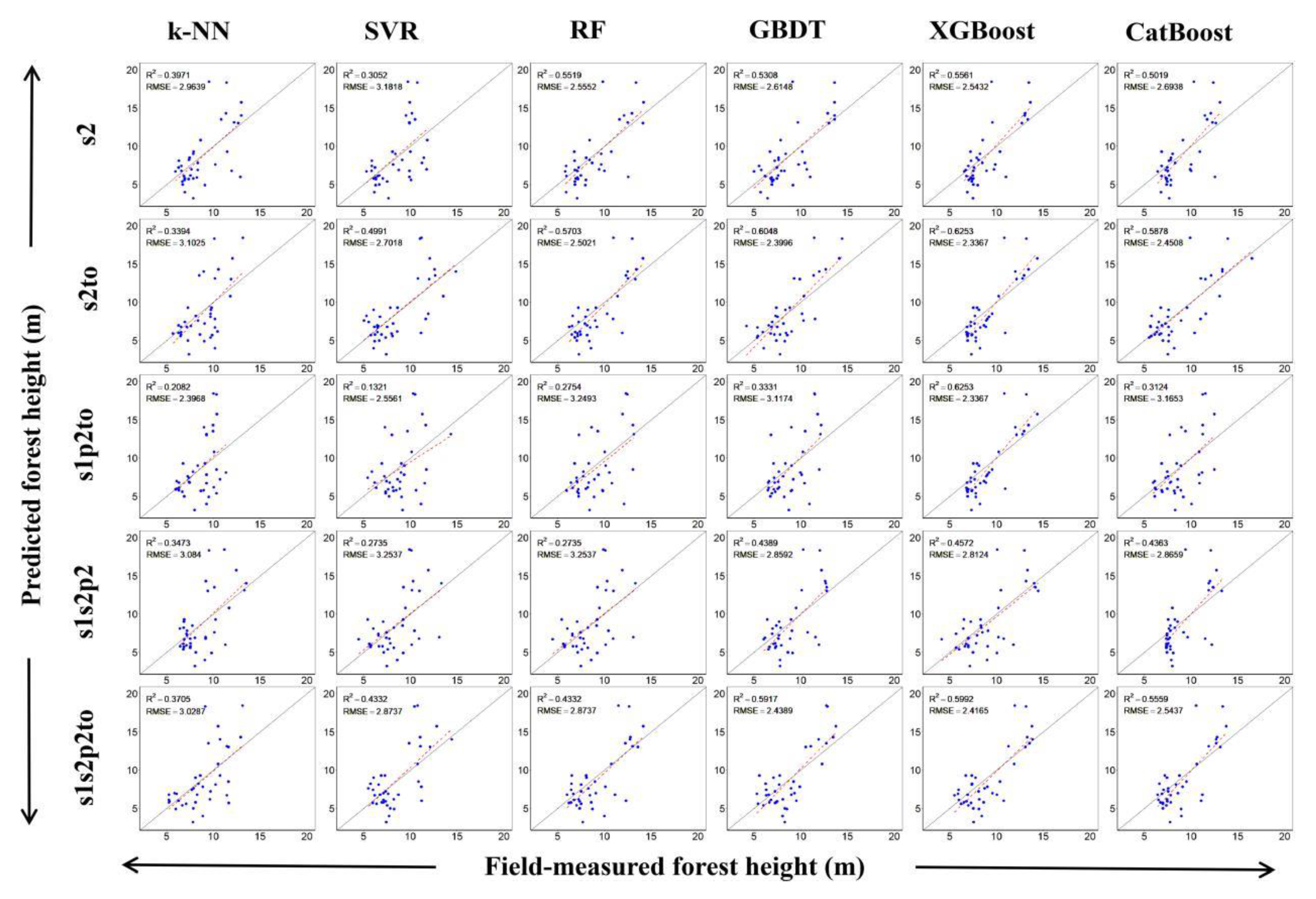
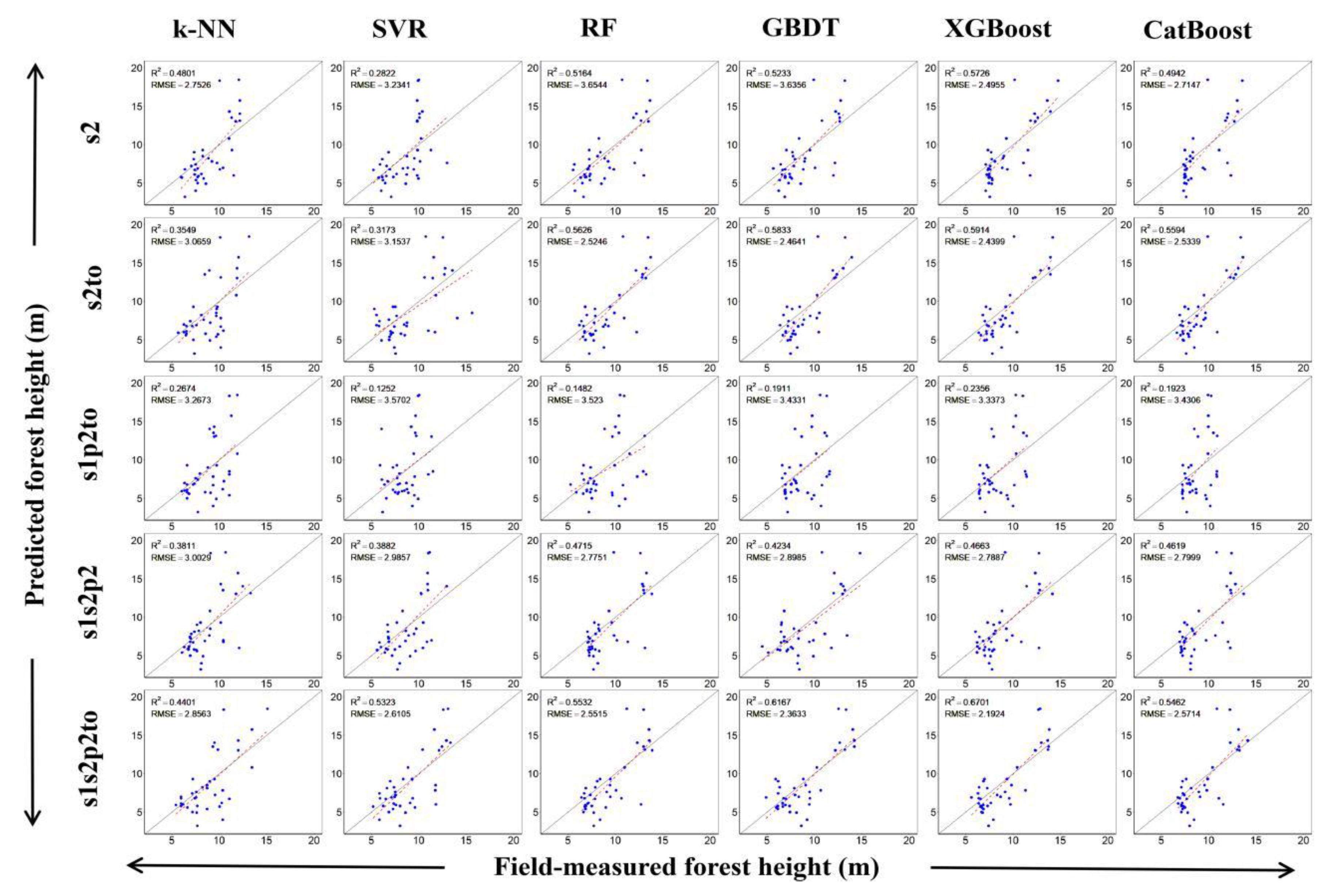
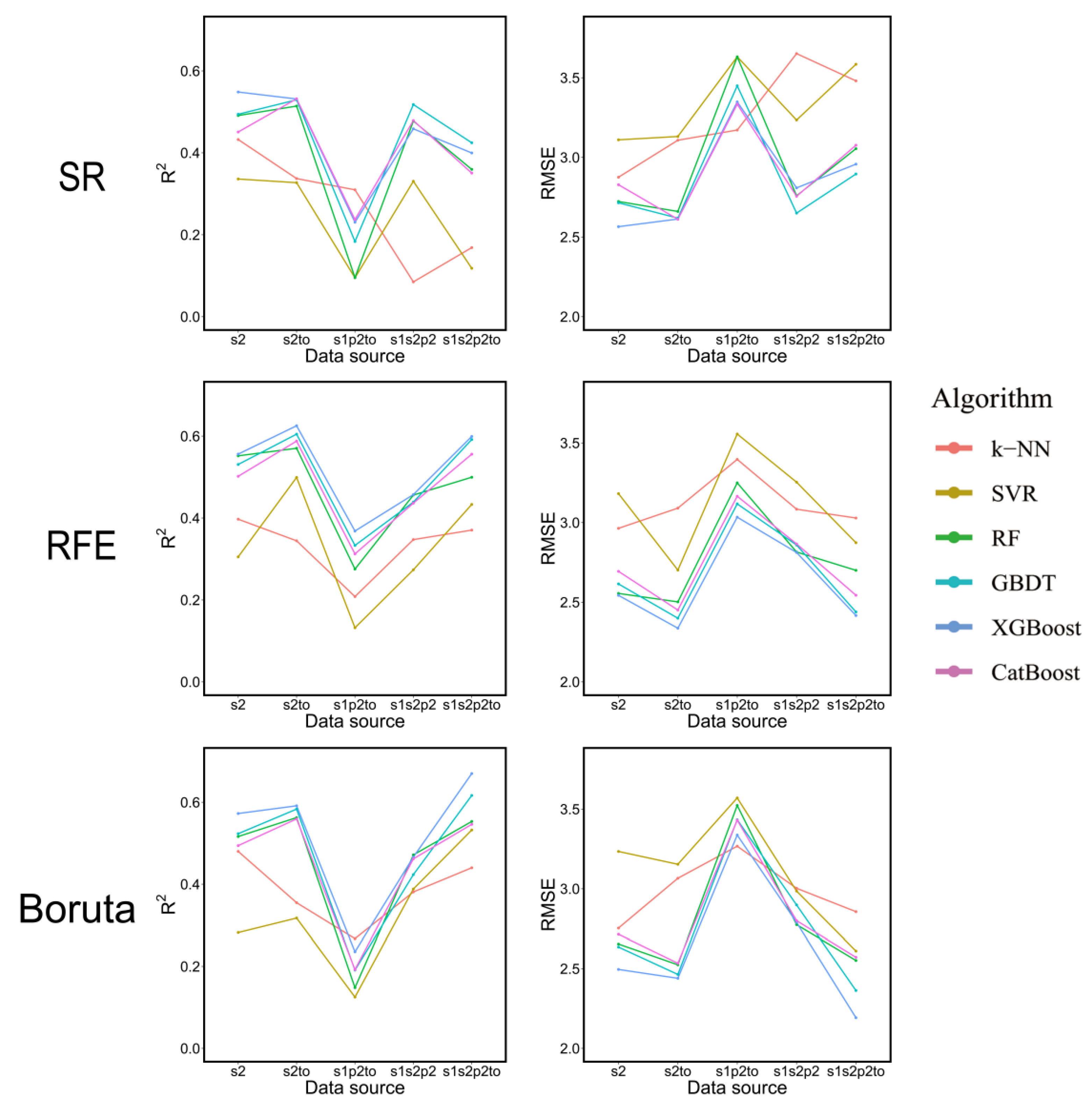
3.2. Forest Height Modeling Results

We applied three statistical metrics (${\mathrm{R}}^2$, RMSE, rRMSE) to evaluate the height models built from different variable scenarios by using the reserved 30% field plot data (

Table 6. Performance of forest height estimation models in the validation datasets.

Data Scenario	Regression Method	Feature Selection Method
		SR			RFE			Boruta
		R2	RMSE (m)	rRMSE (%)	R2	RMSE (m)	rRMSE (%)	R2	RMSE (m)	rRMSE (%)
s2	k-NN	0.43	2.9	33.53	0.40	3.0	34.56	0.48	2.8	32.11
s2	SVR	0.33	3.1	36.27	0.31	3.2	37.10	0.28	3.2	37.71
s2	RF	0.49	2.7	31.75	0.55	2.6	29.80	0.52	2.7	30.95
s2	GBDT	0.49	2.7	31.66	0.53	2.6	30.49	0.52	2.6	30.73
s2	XgBoost	0.55	2.6	29.91	0.56	2.5	29.66	0.57	2.5	29.10
s2	CatBoost	0.45	2.8	32.98	0.50	2.7	31.41	0.49	2.7	31.66
s1s2p2	k-NN	0.08	3.7	42.58	0.35	3.1	35.96	0.38	3.0	35.02
s1s2p2	SVR	0.33	3.2	37.72	0.27	3.3	37.94	0.39	3.0	34.82
s1s2p2	RF	0.48	2.8	32.17	0.46	2.8	32.83	0.47	2.8	32.36
s1s2p2	GBDT	0.52	2.7	30.90	0.44	2.9	33.34	0.42	2.9	33.80
s1s2p2	XgBoost	0.46	2.8	32.75	0.46	2.8	32.80	0.47	2.8	32.52
s1s2p2	CatBoost	0.48	2.8	32.14	0.44	2.9	33.42	0.46	2.8	32.65
s2to	k-NN	0.34	3.1	36.24	0.34	3.1	36.18	0.35	3.1	35.75
s2to	SVR	0.33	3.1	36.51	0.50	2.7	31.51	0.32	3.2	36.77
s2to	RF	0.51	2.7	31.02	0.57	2.5	29.18	0.56	2.5	29.44
s2to	GBDT	0.53	2.6	30.54	0.60	2.4	27.98	0.58	2.5	28.73
s2to	XgBoost	0.53	2.6	30.47	0.63	2.3	27.25	0.59	2.4	28.45
s2to	CatBoost	0.53	2.6	30.45	0.59	2.5	28.58	0.56	2.5	29.55
s1p2to	k-NN	0.31	3.2	36.98	0.21	3.4	39.61	0.27	3.3	38.10
s1p2to	SVR	0.09	3.6	42.35	0.13	3.6	41.47	0.13	3.6	41.63
s1p2to	RF	0.10	3.6	42.34	0.28	3.2	37.89	0.15	3.5	41.08
s1p2to	GBDT	0.18	3.5	40.22	0.33	3.1	36.35	0.19	3.4	40.03
s1p2to	XgBoost	0.23	3.3	39.05	0.37	3.0	35.38	0.24	3.3	38.92
s1p2to	CatBoost	0.24	3.3	38.88	0.31	3.2	36.91	0.19	3.4	40.00
s1s2p2to	k-NN	0.17	3.5	40.59	0.37	3.0	35.32	0.44	2.9	33.31
s1s2p2to	SVR	0.12	3.6	41.80	0.43	2.9	33.51	0.53	2.6	30.44
s1s2p2to	RF	0.36	3.1	35.62	0.50	2.7	31.49	0.55	2.6	29.75
s1s2p2to	GBDT	0.42	2.9	33.77	0.59	2.4	28.44	0.62	2.4	27.56
s1s2p2to	XgBoost	0.40	3.0	34.49	0.60	2.4	28.18	0.67	2.2	25.57
s1s2p2to	CatBoost	0.35	3.1	35.87	0.56	2.5	29.66	0.55	2.6	29.98

).

For five different data scenarios, the optimal models of five data scenarios were from different feature selection methods. In the scenario “s2” and “s1s2p2to”, the models based on Boruta and XGBoost provided the best performance. In the scenario “s2to” and “s1p2to”, the models based RFE and XGBoost outperformed others. In the scenario “s1s2p2”, the model based on SR and GBDT was the best. Furthermore, we found that the difference in the performance between the scenario “s2”, “s1s2p2”, “s2to”, “s1s2p2to” was not very obvious, while the scenarios combining optical and topography variables such as the “s2to” and “s1s2p2to” scenario further improved modeling accuracy overall. Compared with the other four scenarios, the scenario “s1s2p2”, which contained radar and topography feature variables, provided much poorer modeling results.

Interestingly, on the basis of optical variables modeling alone, adding radar-derived variables marginally lowered the modeling accuracy of forest height, while adding topography variables improved the modeling accuracy in most situations. For instance, when combining Boruta and RF for modeling, ${\mathrm{R}}^2$ increased by 8.95% and RMSE decreased by 4.89% after adding topography variables, while ${\mathrm{R}}^2$ decreased by 8.69% and RMSE increased by 4.55% after adding radar variables. When topography variables and radar variables were both added to the optical variables dataset, the modeling results were connected to the technique of feature selection. While selecting feature variables based on SR, the modeling accuracy exhibited an apparent downward trend, regardless of the algorithm utilized; however, the modeling effect was improved when RFE and Boruta were used to screen feature variables, with ${\mathrm{R}}^2$ increased from 0.31–0.56 to 0.37–0.60 based on RFE, ${\mathrm{R}}^2$ increased from 0.28–0.57 to 0.44–0.67 based on Boruta.

Figure 3 shows the broken-line graph based on three different feature selection methods, five different data combinations, and six modeling methods (${\mathrm{R}}^2$ on the left and RMSE on the right). For the three different feature selection methods, the modeling performance of Boruta-based and RFE-based approaches was superior to SR. The ${\mathrm{R}}^2$ and RMSE of SR-based ranged from 0.08 to 0.55, 2.6 to 3.7, respectively, while RFE-based ${\mathrm{R}}^2$ varied from 0.13 to 0.63, RMSE from 2.3 to 3.6, with Boruta-based ${\mathrm{R}}^2$ varying from 0.13 to 0.67, RMSE from 2.2 to 3.6.

For six different modeling methods, it could be seen that when the data source and the method of feature variables selection were consistent, the tree-based ensemble algorithms were always superior to k-NN (with ${\mathrm{R}}^2$ varying from 0.08 to 0.48, RMSE varying from 2.8 to 3.7) and SVR (with ${\mathrm{R}}^2$ varying from 0.09 to 0.53, RMSE varying from 2.6 to 3.6). Among the four ensemble machine learning algorithms, RF (with ${\mathrm{R}}^2$ varying from 0.10 to 0.57, RMSE varying from 2.5 to 3.6), GBDT (with ${\mathrm{R}}^2$ varying from 0.18 to 0.62, RMSE varying from 2.4 to 3.4), XGBoost (with ${\mathrm{R}}^2$ varying from 0.23 to 0.67, RMSE varying from 2.2 to 3.3) and CatBoost (with ${\mathrm{R}}^2$ varying from 0.19 to 0.59, RMSE varying from 2.5 to 3.4), XGBoost’s overall performance was slightly better than the other three. Moreover, in all of the 90 established models, the XGBoost algorithm based on the Boruta feature selection technique in the “s1s2p2to” scenario achieved the best modeling effect (${\mathrm{R}}^2$ = 0.67, RMSE = 2.2 m).

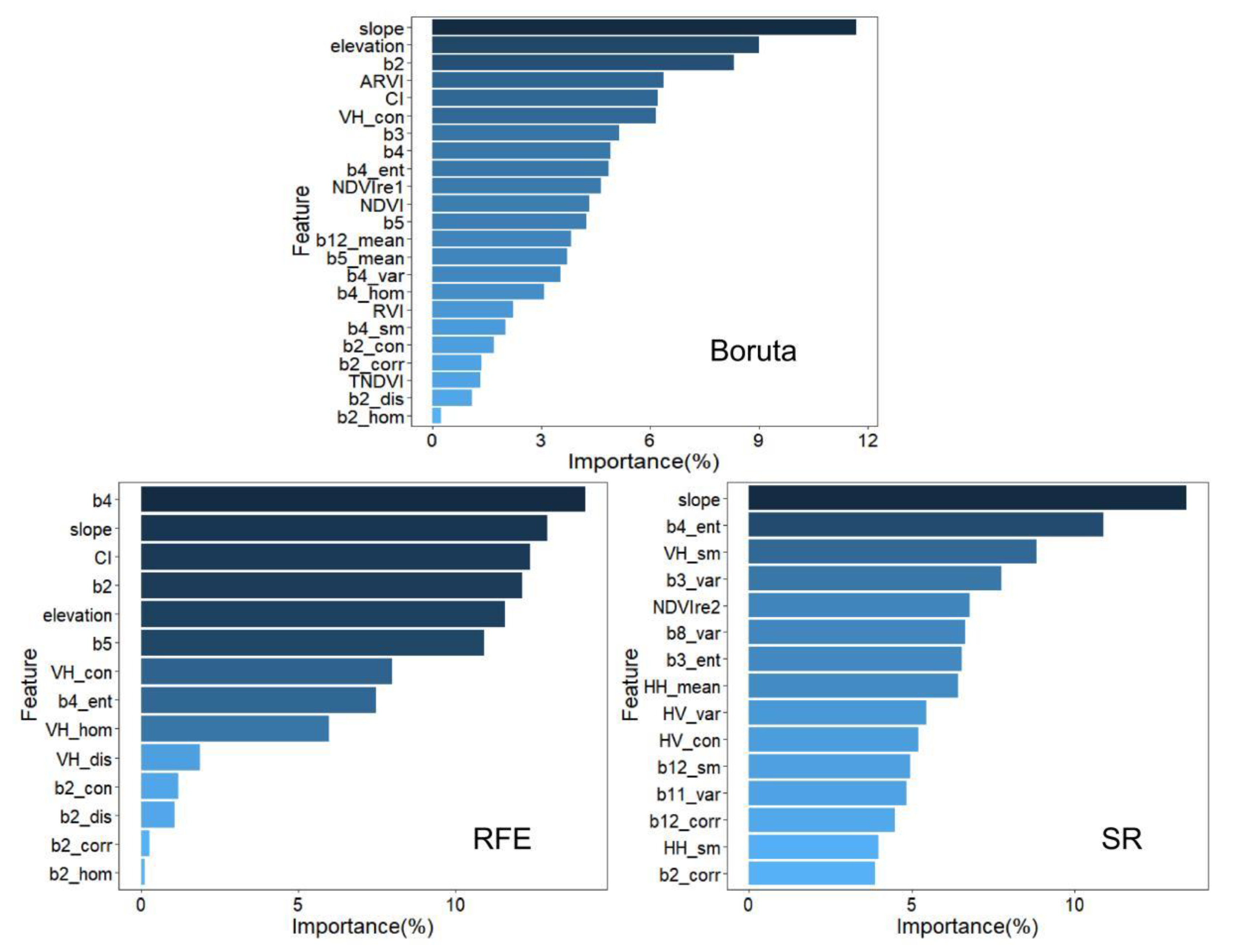
3.3. Variable Importance Analysis

In order to further understand the importance of feature variables in the modeling process, we ranked the importance of “s1s2p2to” scenarios containing all types of feature variables based on the importance ranking method of XGBoost. Figure 4 displays the importance ranking of feature variables based on three distinct feature selection methods.

According to the feature selection method of Boruta and RFE, the terrain-related factors slope and elevation, vegetation index “CI” and band reflectance “b2” and “b4” had relatively high importance, accounting for approximately 40% and 60% of all the selected variables, respectively. Although there were many optical texture feature variables selected, the importance of a single feature was inferior to other features. In addition, although the radar variables selected by these two methods were very few, their significance cannot be completely ignored. Compared with Boruta and RFE, the variables selected by SR were quite different, band reflectance was not chosen, but the optical texture features and the variables derived from PALSAR-2 not considered by Boruta and RFE were taken into account. Thus, it could be seen that different feature selection methods chose different feature variables, and the importance of variables also varies according to different techniques. When using Boruta and RFE, optical variables and terrain variables were more crucial, while the importance of radar variables increased based on SR compared with Boruta and RFE.

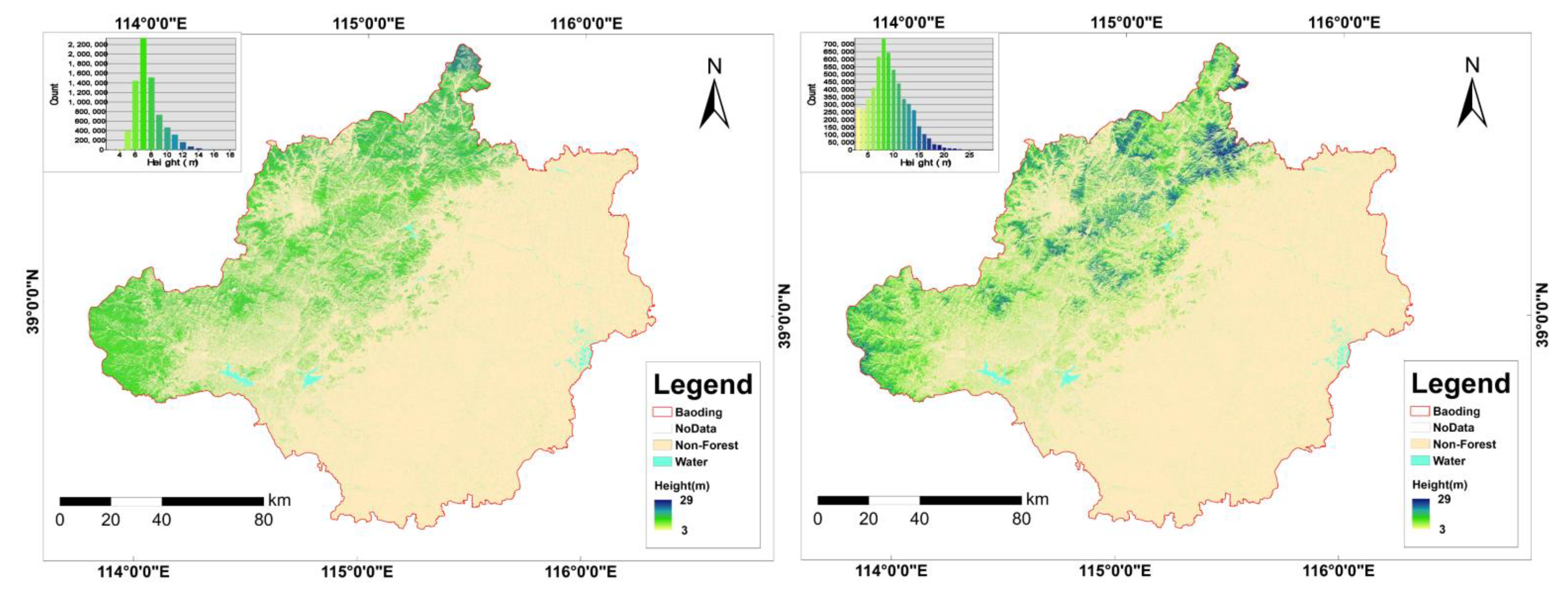
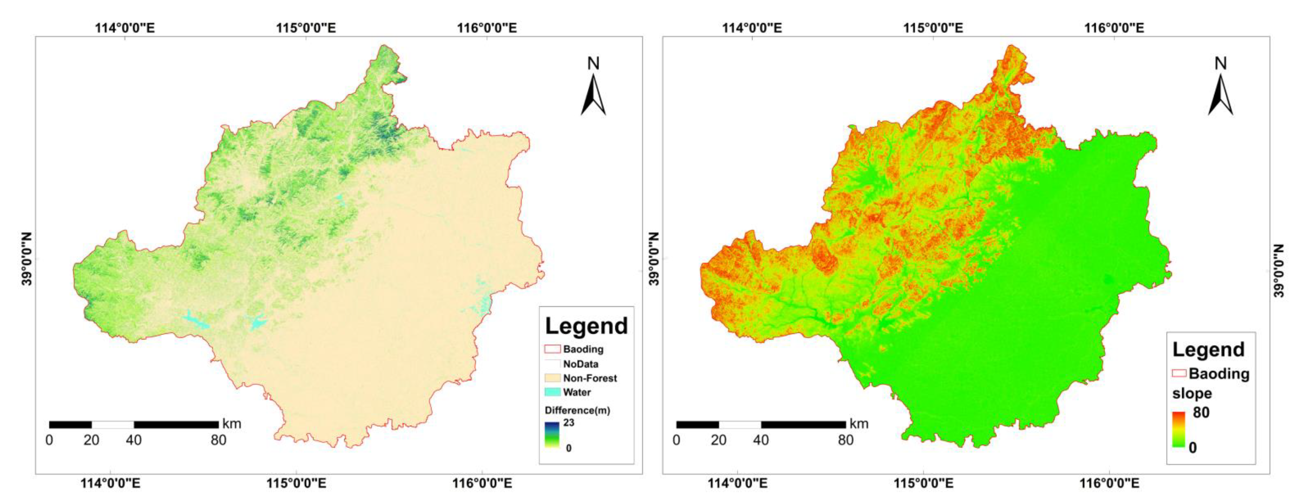
3.4. Forest Height Mapping and Comparison to Existing Product

Based on the modeling results, we combined the feature variables of the scenario “s1s2p2to” selected by Boruta and XGBoost algorithm to produce the forest height wall-to-wall map over Baoding city. According to our forest height map, the value of the forest height in Baoding city was 7.64 ± 1.70 m and ranged from 2.97 m to 17.91 m. We compared our results with the previously released product published by Potapov et al. [40], hereinafter called the “Pota”. According to “Pota”, the forest height in Baoding city was 9.15 ± 3.62 m and ranged from 3.00 m to 29.00 m (

Table 7. Comparison of estimated forest heights over Baoding city.

Product	Nominal Year	Data Source	Nominal Resolution	Algorithm	Forest Height (m)
					Min.	Max.	Mean.	Std.
Map of Potapov	2019	Landsat, GEDI, SRTM	30 m	Regression tree	3.00	29.00	9.15	3.62
Map of this study	2016	Sentinel-1, Sentinel-2, SRTM	25 m	XGBoost	2.97	17.91	7.64	1.70

). Despite the minimum value of the two forest height products being almost identical, the average and maximum values of the “Pota” were much higher than in this study. Moreover, there were notable discrepancies in the distribution of forest height from the two maps of forest height in Baoding city (Figure 5). First, the tree height values of this study were primarily concentrated in the range of 6–8 m, with a normal distribution trend on both sides, whereas the tree height values of “Pota” were mainly distributed in the range of 7–10 m. Second, the higher values of forest height in this study were mainly distributed in the mountainous areas in the north of Baoding city, while according to “Pota”, tall trees were dispersed in both north and west of Baoding. In order to explore the factors that caused the difference between the two maps, we generated a map of forest height differences between these two maps in Baoding city (Figure 6); the average value of the forest height difference was 3.25 m and ranged from 0 to 23.00 m. We found that large differences existed in the mountainous areas in the northern and midwest areas of Baoding city. From the slope distribution map (Figure 6), it could be seen that the areas with big differences were mountainous areas with large slopes and steep terrain. Further counting the difference values above the average difference value in the distribution of different slope levels, we found that the high difference values were primarily distributed in the areas with a slope above 15°, accounting for more than 80% of the total number of high difference values (Figure 7).

4. Discussion

4.1. Performance of Multi-Source Satellite Metrics for Forest Height Estimation

Our study used multi-source satellite data to estimate the forest height of Baoding City. First of all, from the different scenarios of various variable combinations, the variable combination of optical sensor and radar sensor was not always superior to a single optical sensor, which was consistent with the previous research findings when Li et al. applied Landsat 8 and Sentinel-1A data to estimate forest aboveground biomass [75]; however, at the same time, our study results also demonstrated that the performance of the combination of optical, radar, and terrain variables was slightly better than that of a single sensor. Secondly, according to the variables selected by three different feature selection methods and the importance ranking results, optical variables had higher potential than radar variables in estimating forest height, which was supported by Huang et al. [22]. Previous studies have shown that the variables derived from Sentinel-1 and PALSAR-2 were valuable and common predictors for forest height estimation [79,80]; however, in this study, their role was auxiliary, and the accuracy improvement of forest height estimation was not obvious. There were two potential causes to explain this phenomenon. The first was because the C-band SAR has limited penetration of the forest, and is vulnerable to topographic factors in mountainous areas. The second was that the used PALSAR-2 data did not contain the real image at the time of field data collection, but the mosaic image in 2016. The inconsistency between the ground data and the image may result in being not very inaccurate. Furthermore, terrain factors such as elevation were discovered to present good performance in estimating forest height, which was compatible with the earlier research conducted by Xi et al. [81]. Because SRTM employed an InSAR instrument, the vegetation contribution is not totally separated from the ground elevation, so the elevation may include part of the vegetation height information.

4.2. Performance of Different Feature Variable Selection Methods

We explored three different techniques to select feature variables. Table 5 showed that there were certain disparities in quantity and selected variables for different methods. In particular, the variables screened by SR were quite different from those selected by the other two methods. This might be related to the fundamentals of the three approaches. SR is based on AIC information statistics to delete or add variables accomplished by selecting the smallest AIC information statistics. It is worth noting that since the AIC tended to select more parameters than required when using small or medium samples, we mitigated the limitations of the method by removing certain non-essential variables by making the p-value of all selected variables significant (p < 0.05) [55]. RFE and Boruta are methods around the core idea of random forest, so the selected variables had a certain degree of similarity.

Table 8. Average running time and statistical of ${\mathrm{R}}^2$, RMSE, and rRMSE for different variable selection methods.

Method	$${\mathbf{R}}^2$$				RMSE				rRMSE				Average Running Time (s)
	Min.	Max.	Mean.	Std.	Min.	Max.	Mean.	Std.	Min.	Max.	Mean.	Std.
SR	0.08	0.55	0.36	0.15	2.6	3.7	3.0	0.4	29.91	42.58	35.38	4.09	3.68
RFE	0.13	0.63	0.44	0.13	2.2	3.6	2.8	0.3	25.57	41.46	33.13	3.81	3343.77
Boruta	0.13	0.67	0.43	0.15	2.3	3.6	2.9	0.4	27.25	41.63	33.28	4.36	17.75

summarizes statistical data for different variable selection methods. From the mean values shown in the table, the effect of RFE and Boruta was significantly better than SR and the average value of RFE was slightly better than Boruta; however, the calculation time of executing RFE algorithm in “caret” package was much longer than that of Boruta, while its average accuracy improvement was very limited, and the optimal modeling result was also based on Boruta; therefore, from the perspective of modeling accuracy and time efficiency, we considered that Boruta was the best feature selection method in this study. Agjee et al. [82] came to the same conclusion when they compared RFE and Boruta to identify multitemporal hyperspectral data to detect the efficacy of the biocontrol agent.

4.3. Performance of Different Machine Learning Algorithms

Among six machine learning algorithms, four tree-based ensemble algorithms provided better forest height estimation accuracy than the other algorithms, and XGBoost was superior to the other three ensemble algorithms. This result was similar to the research conducted by Arjasakusuma et al. [83] when comparing MARS, SVR extra trees (ET), and extreme gradient boosting (XGB) with trees (XGbtree and XGBdart) and linear (XGBlin) classifiers for modeling forest height from the combination of LiDAR and hyperspectral data. Comparable conclusions were drawn in the studies of forest aboveground biomass estimation. Pham et al. [43] combined genetic algorithm (GA) and XGBoost to achieve optimal mangrove AGB estimation than the other four ML algorithms (RF, SRM, GBRT, and CatBoost); Li et al. [74] combined China’s national forest inventory, Landsat-8 data, and LR, RF, and XGBoost algorithms to establish AGB models and found that the XGBoost model significantly improved the estimation accuracy and reduced the problem of overestimation and underestimation to a certain extent.

The reasons why the XGBoost model performed well included two aspects. First, XGBoost is a flexible algorithm that can correct residual errors to generate a new tree based on the previous trees. Second, the XGBoost model is an advanced gradient boosting system, which improves the processing of regularization learning objectives and avoids overfitting; however, it is worth noting that all the machine learning algorithms cannot entirely address the problem of overestimation and underestimation of forest height. In the present study, XGBoost achieved the optimal solution, but its potential in the face of various geographical situations requires further investigation.

4.4. Important Factors Analyze in Forest Height Estimation

Numerous factors can influence the accuracy of forest height estimation. In the present study, we employed ANOVA analysis to evaluate the impact of data source, feature selection method, regression algorithm, and their interaction on forest height estimation. To better illustrate how each factor explained the total variance, we calculated the ratio of the sum of squares of each factor to the total sum of squares (η2). According to the ANOVA results (

Table 9. ANOVA results of the ${\mathrm{R}}^2$, RMSE, and rRMSE for three different factors.

Factor	Df	R2			RMSE			rRMSE
		SumSq	η2	Pr (>F)	SumSq	η2	Pr (>F)	SumSq	η2	Pr (>F)
Data source	4	0.90	0.47	<2.2 × 10−16 ***	5.30	0.46	2.571 × 10−07 ***	720.87	0.46	2.571 × 10−07 ***
Feature selection method	2	0.11	0.06	2.147 × 10−06 ***	0.70	0.06	<2.2 × 10−16 ***	95.02	0.06	<2.2 × 10−16 ***
Regression algorithm	5	0.45	0.24	1.345 × 10−12 ***	2.86	0.25	4.992 × 10−14 ***	389.54	0.25	4.992 × 10−14 ***
Data source Feature selection method	8	0.16	0.08	1.412 × 10−05 ***	1.00	0.09	1.860 × 10−06 ***	136.25	0.09	1.860 × 10−06 ***
Data source Regression algorithm	20	0.14	0.07	0.01107 *	0.85	0.07	0.003017 **	115.79	0.07	0.003017 **
Feature selection method Regression algorithm	10	0.02	0.01	0.84356	0.09	0.01	0.826854	11.96	0.01	0.826854
Residuals	40	0.12			0.62			83.68

Signif. Codes: ‘***’: 0; ‘**’: 0.001; ‘*’: 0.01.

), the data source was the most influential factor, accounting for 47% of the total variance of ${\mathrm{R}}^2$, 46% of RMSE and 46% of rRMSE. Then regression algorithm explained 24% of the total variance of ${\mathrm{R}}^2$, 25% of RMSE and 25% of rRMSE. The influence of the feature selection method and the interaction between the three factors was relatively low, altogether accounting for approximate 20% of the total variance in ${\mathrm{R}}^2$, RMSE, and rRMSE. However, it is worth mentioning that the feature selection method, the interaction between data source and feature selection method, and the interaction between data source and regression algorithm also had a significant effect on the results of ${\mathrm{R}}^2$, RMSE, and rRMSE, so these three factors, including data source, feature selection, and regression algorithm could not be disregarded. In a word, it is necessary to take these three factors into account in the estimation of forest height.

4.5. Map Product Comparison

Previous studies had shown that complex terrain increased uncertainty in forest height estimation and the accuracy of forest height estimates decreased with increasing slope values [84,85]. In rugged mountainous areas, the radar’s backscatter coefficients and optical spectral reflectance information were susceptible to terrain, and the GEDI used in Potapov’s study, whose signals were also skewed by the intricate topographical conditions within its footprint. The combination of these effects led to the large difference in values between Potapov’s map and our map, mainly in the areas with high slope values. Furthermore, the result of our research showed an obvious underestimation of the high forest height value. We explained this phenomenon by concentrating on two reasons. The first reason was that optical data mainly captured forest spectral information, with the SAR data of C/L-Band limited ability to penetrate forest canopy, causing their signals to appear saturated. Secondly, due to the small quantity values at the high altitude of our field plots, the high values will be underestimated in the process of machine learning modeling. Potapov reported oversampling of tall trees in their overall reference data set resulted in high values that could be overestimated to some extent. This conclusion was also verified in our study that the average and maximum tree height values in “Pota” were greater than field data.

4.6. Recent Related Works Comparison

Compared with two recent studies which used both optical and radar variables for forest tree height estimation, the similarity was that all three studies estimated forest height by constructing an empirical model between forest height and multi-source remote sensing information [22,23]. The difference was that Liu et al. [23] constructed a simple logarithmic regression to estimate forest height based on the relationship between forest height and the backscattering coefficients derived from Sentinel-1 data and the fraction of vegetation cover derived from Sentinel-2 data with the results ${\mathrm{R}}^2$ = 0.53414 and RMSE = 2.9156 m, while Huang et al. [22] and our study both extracted considerable feature variables and employed different feature selection methods and regression algorithms to estimate forest height. Huang et al. systematically evaluated the performance of different remote sensing metrics, feature selection methods, and regression algorithms by dividing the extracted feature variables into ten scenarios and using two types of variable selection methods and three types of regression models; the best estimation was achieved by RF models with ${\mathrm{R}}^2$ ranged from 0.47 to 0.52, RMSE ranged from 3.8 to 5.3 m, whereas in our study, we utilized four types of remote sensing data, three feature selection methods, and six machine learning algorithms and applied the ANOVA to quantify the importance of these factors on forest height estimation; the variables selected based on Boruta including Sentinel-1, Sentinel-2, and topography metrics, combined with the XGBoost algorithm provided the optimal model (${\mathrm{R}}^2$ = 0.67, RMSE = 2.2 m).

4.7. Limitations and Prospects

In this study, we found that all the models had the problem of high-value underestimation. From the scatter plot (Figure A1, Figure A2 and Figure A3), we could see intuitively the predicted value was below the center line when the tree height exceeded 15 m which meant that despite using multi-sensor datasets to decrease estimation error, the model still underestimated at higher tree heights. In light of this issue, we proposed the following potential improvement directions. (1) Optical sensor such as Sentinel-2 used in this study has some issues, such as poor sensitivity and easy saturation to dense vegetation information, and SAR data, such as Sentinel-1 and PALSAR-2, are susceptible to topography and other factors, and the backscattering information has the problem of signal saturation. As a result, lidar data with direct detection capabilities of forest vertical structures can be combined with optical and SAR data in future studies to increase the accuracy of regional forest height estimation. (2) Previous studies showed modeling based on different forest types and tree height levels can lessen the model’s dependence on training samples and improve the modeling effect [81,86]. Due to a lack of sample plot data, we were unable to address forest types or tree height levels to undertake to model respectively. In the future, with sufficient plot data gathered, these strategies can be applied to minimize the uncertainty in the modeling process. (3) Since most machine learning models are black-box models, they are difficult to reflect the mechanism and process between forest parameters and remote sensing information, and the interpretability for reality is weak. The improvement of the generalizability and accuracy of forest parameter estimation by simply constructing empirical models is limited. Physical geography, bioclimatic and cultural conditions are proved to be crucial for the estimation of forest parameters [67,84]; therefore, in subsequent studies, zoning and stratification strategies or coupling remote sensing data and forest physiological process models should be emphasized to estimate forest height and other parameters.

5. Conclusions

In this study, we produced a 25 m spatial resolution wall-to-wall map of the forest height in Baoding, north China and assessed the impacts of three aspects on forest height estimation utilizing Sentinel-1, Sentinel-2, PALSAR 2 mosaic, SRTM DEM, and the NFCI data, three feature selection methods (SR, RFE, and Boruta), and six machine learning algorithms (k-NN, SVM, RF, GBDT, XGBoost, and CatBoost). The results of ANOVA analysis demonstrated that data source, feature selection method, and machine learning algorithm significantly influenced the results of forest height estimation. The accuracy with optical data alone was slightly lower than the combined data of multiple sensors, and multi-source data could improve the estimation accuracy to a certain extent. Optical and topographic indicators were proved to be more effective than that radar indicators. The subset of features screened by RFE and Boruta varied greatly from SR, and the models exhibited from the variables screened based on RFE and Boruta had better performance compared with SR. Moreover, XGBoost outperformed the other five machine learning algorithms. Ultimately, we obtained the optimal model (${\mathrm{R}}^2$ = 0.67, RMSE = 2.2 m) based on the combination of Sentinel-1, Sentinel-2, and topography data using Boruta and XGBoost algorithms. The generated forest height map differed from the existing map product, and the regions with large differences between the two maps were mostly distributed in the steep areas with high slope values. Overall, our findings provided a solution for the subsequent forest height mapping at larger scales (national or global) with high precision.

References

1. Achard, F.; Eva, H.; Stibig, H.; Mayaux, P.; Gallego, J.; Richards, T.; Malingreau, J. Determination of Deforestation Rates of the World’s Humid Tropical Forests. Science 2002, 297, 999–1002. [Google Scholar] [CrossRef] [PubMed]
2. Dong, J.; Kaufmann, R.; Myneni, R.; Tucker, C.; Kauppi, P.; Liski, J.; Buermann, W.; Alexeyev, V.; Hughes, M. Remote sensing estimates of boreal and temperate forest woody biomass: Carbon pools, sources, and sinks. Remote Sens. Environ. 2003, 84, 393–410. [Google Scholar] [CrossRef]
3. Huang, H.; Liu, C.; Wang, X.; Zhou, X.; Gong, P. Integration of multi-resource remotely sensed data and allometric models for forest aboveground biomass estimation in China. Remote Sens. Environ. 2019, 221, 225–234. [Google Scholar] [CrossRef]
4. Hurtt, G.; Zhao, M.; Sahajpal, R.; Armstrong, A.; Birdsey, R.; Campbell, E.; Dolan, K.; Dubayah, R.; Fisk, J.; Flanagan, S.; et al. Beyond MRV: High-resolution forest carbon modeling for climate mitigation planning over Maryland, USA. Environ. Res. Lett. 2019, 14, 045013. [Google Scholar] [CrossRef]
5. Herold, M.; Carter, S.; Avitabile, V.; Espejo, A.; Jonckheere, I.; Lucas, R.; McRoberts, R.; Næsset, E.; Nightingale, J.; Petersen, R.; et al. The Role and Need for Space-Based Forest Biomass-Related Measurements in Environmental Management and Policy. Surv. Geophys. 2019, 40, 757–778. [Google Scholar] [CrossRef]
6. Duncanson, L.; Armston, J.; Disney, M.; Avitabile, V.; Barbier, N.; Calders, K.; Carter, S.; Chave, J.; Herold, M.; Crowther, T.; et al. The Importance of Consistent Global Forest Aboveground Biomass Product Validation. Surv. Geophys. 2019, 40, 979–999. [Google Scholar] [CrossRef]
7. Wulder, M.; White, J.; Nelson, R.; Næsset, E.; Ørka, H.; Coops, N.; Hilker, T.; Bater, C.; Gobakken, T. Lidar sampling for large-area forest characterization: A review. Remote Sens. Environ. 2012, 121, 196–209. [Google Scholar] [CrossRef]
8. Hansen, M.; Potapov, P.; Goetz, S.; Turubanova, S.; Tyukavina, A.; Krylov, A.; Kommareddy, A.; Egorov, A. Mapping tree height distributions in Sub-Saharan Africa using Landsat 7 and 8 data. Remote Sens. Environ. 2016, 185, 221–232. [Google Scholar] [CrossRef]
9. Wolter, P.; Townsend, P.; Sturtevant, B. Estimation of forest structural parameters using 5 and 10 meter SPOT-5 satellite data. Remote Sens. Environ. 2009, 113, 2019–2036. [Google Scholar] [CrossRef]
10. Potapov, P.; Tyukavina, A.; Turubanova, S.; Talero, Y.; Hernandez-Serna, A.; Hansen, M.; Saah, D.; Tenneson, K.; Poortinga, A.; Aekakkararungroj, A.; et al. Annual continuous fields of woody vegetation structure in the Lower Mekong region from 2000–2017 Landsat time-series. Remote Sens. Environ. 2019, 232, 111278. [Google Scholar] [CrossRef]
11. Simard, M.; Pinto, N.; Fisher, J.; Baccini, A. Mapping forest canopy height globally with spaceborne lidar. J. Geophys. Res. 2011, 116, 4021. [Google Scholar] [CrossRef]
12. Liang, X.; Kankare, V.; Hyyppä, J.; Wang, Y.; Kukko, A.; Haggrén, H.; Yu, X.; Kaartinen, H.; Jaakkola, A.; Guan, F.; et al. Terrestrial laser scanning in forest inventories. ISPRS J. Photogramm. Remote Sens. 2016, 115, 63–77. [Google Scholar] [CrossRef]
13. Alexander, C.; Korstjens, A.; Hill, R. Influence of micro-topography and crown characteristics on tree height estimations in tropical forests based on LiDAR canopy height models. Int. J. Appl. Earth Obs. Geoinf. 2018, 65, 105–113. [Google Scholar] [CrossRef]
14. Almeida, D.; Broadbent, E.; Zambrano, A.; Wilkinson, B.; Ferreira, M.; Chazdon, R.; Meli, P.; Gorgens, E.; Silva, C.; Stark, S.; et al. Monitoring the structure of forest restoration plantations with a drone-lidar system. Int. J. Appl. Earth Obs. Geoinf. 2019, 79, 192–198. [Google Scholar] [CrossRef]
15. Zhang, Z.; Ni, W.; Sun, G.; Huang, W.; Ranson, K.J.; Cook, B.D.; Guo, Z. Biomass retrieval from L-band Polarimetric UAVSAR Backscatter and prism stereo imagery. Remote Sens. Environ. 2017, 194, 331–346. [Google Scholar] [CrossRef]
16. Qi, W.; Lee, S.-K.; Hancock, S.; Luthcke, S.; Tang, H.; Armston, J.; Dubayah, R. Improved Forest height estimation by fusion of simulated GEDI LIDAR data and TanDEM-X Insar Data. Remote Sens. Environ. 2019, 221, 621–634. [Google Scholar] [CrossRef]
17. Li, C.; Song, J.; Wang, J. New approach to calculating tree height at the regional scale. For. Ecosyst. 2021, 8, 24. [Google Scholar] [CrossRef]
18. Popescu, S.C. Estimating biomass of individual pine trees using airborne lidar. Biomass Bioenergy 2007, 31, 646–655. [Google Scholar] [CrossRef]
19. Lang, N.; Schindler, K.; Wegner, J.D. Country-wide high-resolution vegetation height mapping with sentinel-2. Remote Sens. Environ. 2019, 233, 111347. [Google Scholar] [CrossRef]
20. Neumann, M.; Ferro-Famil, L.; Reigber, A. Estimation of Forest Structure, Ground, and Canopy Layer Characteristics from Multibaseline Polarimetric Interferometric SAR Data. IEEE Trans. Geosci. Remote Sens. 2010, 48, 1086–1104. [Google Scholar] [CrossRef] [Green Version]
21. López-Serrano, P.M.; López-Sánchez, C.A.; Álvarez-González, J.G.; García-Gutiérrez, J. A Comparison of Machine Learning Techniques Applied to Landsat-5 TM Spectral Data for Biomass Estimation. Can. J. Remote Sens. 2016, 42, 690–705. [Google Scholar] [CrossRef]
22. Huang, W.; Min, W.; Ding, J.; Liu, Y.; Hu, Y.; Ni, W.; Shen, H. Forest height mapping using inventory and multi-source satellite data over Hunan Province in southern China. For. Ecosyst. 2022, 9, 100006. [Google Scholar] [CrossRef]
23. Liu, Y.; Gong, W.; Xing, Y.; Hu, X.; Gong, J. Estimation of the forest stand mean height and aboveground biomass in northeast China using SAR Sentinel-1B, multispectral sentinel-2a, and DEM imagery. ISPRS J. Photogramm. Remote Sens. 2019, 151, 277–289. [Google Scholar] [CrossRef]
24. Amini, J.; Sumantyo, J.T.S. Employing a Method on SAR and Optical Images for Forest Biomass Estimation. IEEE Trans. Geosci. Remote Sens. 2009, 47, 4020–4026. [Google Scholar] [CrossRef]
25. Forkuor, G.; Benewinde Zoungrana, J.-B.; Dimobe, K.; Ouattara, B.; Vadrevu, K.P.; Tondoh, J.E. Above-ground biomass mapping in West African dryland forest using Sentinel-1 and 2 datasets—A case study. Remote Sens. Environ. 2020, 236, e111496. [Google Scholar] [CrossRef]
26. Li, H.; Kato, T.; Hayashi, M.; Wu, L. Estimation of forest aboveground biomass of two major conifers in Ibaraki Prefecture, Japan, from palsar-2 and sentinel-2 data. Remote Sens. 2022, 14, 468. [Google Scholar] [CrossRef]
27. Lu, D.; Chen, Q.; Wang, G.; Li, G.; Moran, E. A survey of remote sensing-basedd aboveground biomass estimation methods in forest ecosystems. Int. J. Digit. Earth. 2016, 9, 63–105. [Google Scholar] [CrossRef]
28. Li, X.; Lin, H.; Long, J.; Xu, X. Mapping the growing stem volume of the coniferous plantations in north China using multispectral data from integrated GF-2 and sentinel-2 images and an optimized feature variable selection method. Remote Sens. 2021, 13, 2740. [Google Scholar] [CrossRef]
29. Li, G.; Xie, Z.; Jiang, X.; Lu, D.; Chen, E. Integration of ZiYuan-3 Multispectral and Stereo Data for Modeling Aboveground Biomass of Larch Plantations in North China. Remote Sens. 2019, 11, 2328. [Google Scholar] [CrossRef]
30. Zhao, P.; Lu, D.; Wang, G.; Liu, L.; Li, D.; Zhu, J.; Yu, S. Forest aboveground biomass estimation in Zhejiang Province using the integration of Landsat TM and ALOS PALSAR data. Int. J. Appl. Earth Obs. 2016, 53, 1–15. [Google Scholar] [CrossRef]
31. Wang, X.; Liu, C.; Lv, G.; Xu, J.; Cui, G. Integrating multi-source remote sensing to assess forest aboveground biomass in the Khingan mountains of north-eastern China using machine-learning algorithms. Remote Sens. 2022, 14, 1039. [Google Scholar] [CrossRef]
32. Purohit, S.; Aggarwal, S.P.; Patel, N.R. Estimation of forest aboveground biomass using combination of Landsat 8 and sentinel-1a data with random forest regression algorithm in Himalayan foothills. Trop. Ecol. 2021, 62, 288–300. [Google Scholar] [CrossRef]
33. Peng, X.; Zhao, A.; Chen, Y.; Chen, Q.; Liu, H.; Wang, J.; Li, H. Comparison of modeling algorithms for Forest Canopy Structures based on UAV-LIDAR: A case study in tropical China. Forests 2020, 11, 1324. [Google Scholar] [CrossRef]
34. Zhao, Q.; Yu, S.; Zhao, F.; Tian, L.; Zhao, Z. Comparison of machine learning algorithms for Forest parameter estimations and application for Forest Quality Assessments. For. Ecol. Manag. 2019, 434, 224–234. [Google Scholar] [CrossRef]
35. Chen, M.; Qiu, X.; Zeng, W.; Peng, D. Combining sample plot stratification and machine learning algorithms to improve forest aboveground carbon density estimation in northeast China using Airborne Lidar Data. Remote Sens. 2022, 14, 1477. [Google Scholar] [CrossRef]
36. Yu, G.; Lu, Z.; Lai, Y. Comparative Study on Variable Selection Approaches in Establishment of Remote Sens. Model for Forest Biomass Estimation. Remote Sens. 2019, 11, 1437. [Google Scholar] [CrossRef]
37. Luo, M.; Wang, Y.; Xie, Y.; Zhou, L.; Qiao, J.; Qiu, S.; Sun, Y. Combination of feature selection and CatBoost for prediction: The first application to the estimation of aboveground biomass. Forests 2021, 12, 216. [Google Scholar] [CrossRef]
38. Ahmed, O.S.; Franklin, S.E.; Wulder, M.A.; White, J.C. Extending airborne lidar-derived estimates of forest canopy cover and height over large areas using KNN with Landsat Time Series Data. IEEE J. Sel. Top. Appl. Earth Obs. Remote Sens. 2016, 9, 3489–3496. [Google Scholar] [CrossRef]
39. Özçelik, R.; Diamantopoulou, M.J.; Crecente-Campo, F.; Eler, U. Estimating crimean juniper tree height using nonlinear regression and artificial neural network models. For. Ecol. Manag. 2013, 306, 52–60. [Google Scholar] [CrossRef]
40. Potapov, P.; Li, X.; Hernandez-Serna, A.; Tyukavina, A.; Hansen, M.C.; Kommareddy, A.; Pickens, A.; Turubanova, S.; Tang, H.; Silva, C.E.; et al. Mapping global forest canopy height through integration of Gedi and Landsat Data. Remote Sens. Environ. 2021, 253, 112165. [Google Scholar] [CrossRef]
41. Wang, M.; Sun, R.; Xiao, Z. Estimation of forest canopy height and aboveground biomass from Spaceborne Lidar and landsat imageries in Maryland. Remote Sens. 2018, 10, 344. [Google Scholar] [CrossRef]
42. Wang, Y.; Li, G.; Ding, J.; Guo, Z.; Tang, S.; Wang, C.; Huang, Q.; Liu, R.; Chen, J.M. A combined glas and Modis estimation of the global distribution of mean forest canopy height. Remote Sens. Environ. 2016, 174, 24–43. [Google Scholar] [CrossRef]
43. Pham, T.D.; Yokoya, N.; Xia, J.; Ha, N.T.; Le, N.N.; Nguyen, T.T.T.; Dao, T.H.; Vu, T.T.P.; Pham, T.D.; Takeuchi, W. Comparison of Machine Learning Methods for Estimating Mangrove Above-Ground Biomass Using Multiple Source Remote Sens. Data in the Red River Delta Biosphere Reserve, Vietnam. Remote Sens. 2020, 12, 1334. [Google Scholar] [CrossRef]
44. Zhang, Y.; Ma, J.; Liang, S.; Li, X.; Liu, J. A stacking ensemble algorithm for improving the biases of forest aboveground biomass estimations from multiple remotely sensed datasets. GIsci. Remote Sens. 2022, 59, 234–249. [Google Scholar] [CrossRef]
45. Gorelick, N.; Hancher, M.; Dixon, M.; Ilyushchenko, S.; Thau, D.; Moore, R. Google Earth Engine: Planetary-scale geospatial analysis for everyone. Remote Sens. Environ. 2017, 202, 18–27. [Google Scholar] [CrossRef]
46. Mullissa, A.; Vollrath, A.; Odongo-Braun, C.; Slagter, B.; Balling, J.; Gou, Y.; Gorelick, N.; Reiche, J. Sentinel-1 SAR Backscatter Analysis Ready Data Preparation in Google Earth Engine. Remote Sens. 2021, 13, 1954. [Google Scholar] [CrossRef]
47. The Japan Aerospace Exploration Agency(JAXA). Global 25m Resolution PALSAR-2/PALSAR Mosaic and Forest/Non-Forest Map (FNF) Dataset Description; JAXA: Tsukuba, Japan, 2019. [Google Scholar]
48. Gong, P.; Liu, H.; Zhang, M.; Li, C.; Wang, J.; Huang, H.; Clinton, N.; Ji, L.; Li, W.; Bai, Y.; et al. Stable classification with limited sample: Transferring a 30-M resolution sample set collected in 2015 to mapping 10-M resolution global land cover in 2017. Sci. Bull. 2019, 64, 370–373. [Google Scholar] [CrossRef]
49. Hu, Y.; Xu, X.; Wu, F.; Sun, Z.; Xia, H.; Meng, Q.; Huang, W.; Zhou, H.; Gao, J.; Li, W.; et al. Estimating Forest Stock Volume in Hunan Province, China, by integrating in situ plot data, sentinel-2 images, and linear and machine learning regression models. Remote Sens. 2020, 12, 186. [Google Scholar] [CrossRef]
50. Frampton, W.J.; Dash, J.; Watmough, G.; Milton, E.J. Evaluating the capabilities of Sentinel-2 for quantitative estimation of biophysical variables in vegetation. ISPRS J. Photogramm. Remote Sens. 2013, 82, 83–92. [Google Scholar] [CrossRef]
51. Vaglio Laurin, G.; Pirotti, F.; Callegari, M.; Chen, Q.; Cuozzo, G.; Lingua, E.; Notarnicola, C.; Papale, D. Potential of ALOS2 and NDVI to Estimate Forest Above-Ground Biomass, and Comparison with Lidar-Derived Estimates. Remote Sens. 2017, 9, 18. [Google Scholar] [CrossRef] [Green Version]
52. Zhang, Y.; Liang, S.; Sun, G. Forest biomass mapping of northeastern China using GLAS and MODIS data. IEEE J. Sel. Top. Appl. Earth Obs. Remote Sens. 2014, 7, 140–152. [Google Scholar] [CrossRef]
53. Chi, H.; Sun, G.; Huang, J.; Guo, Z.; Ni, W.; Fu, A. National forest aboveground biomass mapping from ICESat/GLAS data and MODIS imagery in China. Remote Sens. 2015, 7, 5534–5564. [Google Scholar] [CrossRef]
54. Whittingham, M.J.; Stephens, P.A.; Bradbury, R.B.; Freckleton, R.P. Why do we still use stepwise modelling in ecology and behaviour? J. Anim. Ecol. 2006, 75, 1182–1189. [Google Scholar] [CrossRef]
55. Adame-Campos, R.L.; Ghilardi, A.; Gao, Y.; Paneque-Gálvez, J.; Mas, J. Variables Selection for Aboveground Biomass Estimations Using Satellite Data: A Comparison between Relative Importance Approach and Stepwise Akaike’s Information Criterion. ISPRS Int. J. Geo-Inf. 2019, 8, 245. [Google Scholar] [CrossRef]
56. Venables, W.N.; Ripley, B.D.; Venables, W.N. Modern Applied Statistics with S; Springer: New York, NY, USA, 2002. [Google Scholar]
57. Pullanagari, R.; Kereszturi, G.; Yule, I. Integrating airborne hyperspectral, topographic, and soil data for estimating pasture quality using recursive feature elimination with random forest regression. Remote Sens. 2018, 10, 1117. [Google Scholar] [CrossRef]
58. Zhou, Q.; Zhou, H.; Zhou, Q.; Yang, F.; Luo, L. Structure damage detection based on random forest recursive feature elimination. Mech. Syst. Signal Process. 2014, 46, 82–90. [Google Scholar] [CrossRef]
59. Granitto, P.M.; Furlanello, C.; Biasioli, F.; Gasperi, F. Recursive feature elimination with random forest for ptr-ms analysis of agroindustrial products. Chemom. Intell. Lab. Syst. 2006, 83, 83–90. [Google Scholar] [CrossRef]
60. Kursa, M.B.; Rudnicki, W.R. Feature Selection with the Boruta Package. J. Stat. Softw. 2010, 36, 1–13. [Google Scholar] [CrossRef]
61. Chirici, G.; Barbati, A.; Corona, P.; Marchetti, M.; Travaglini, D.; Maselli, F.; Bertini, R. Non-parametric and parametric methods using satellite images for estimating growing stock volume in Alpine and mediterranean forest ecosystems. Remote Sens. Environ. 2008, 112, 2686–2700. [Google Scholar] [CrossRef]
62. Chirici, G.; Mura, M.; McInerney, D.; Py, N.; Tomppo, E.O.; Waser, L.T.; Travaglini, D.; McRoberts, R.E. A meta-analysis and review of the literature on the K-nearest neighbors technique for forestry applications that use remotely sensed data. Remote Sens. Environ. 2016, 176, 282–294. [Google Scholar] [CrossRef]
63. Mountrakis, G.; Im, J.; Ogole, C. Support Vector Machines in remote sensing: A Review. ISPRS J. Photogramm. Remote Sens. 2011, 66, 247–259. [Google Scholar] [CrossRef]
64. Vafaei, S.; Soosani, J.; Adeli, K.; Fadaei, H.; Naghavi, H.; Pham, T.; Tien Bui, D. Improving accuracy estimation of forest aboveground biomass based on incorporation of Alos-2 palsar-2 and sentinel-2a imagery and Machine Learning: A case study of the hyrcanian forest area (Iran). Remote Sens. 2018, 10, 172. [Google Scholar] [CrossRef]
65. Deb, D.; Deb, S.; Chakraborty, D.; Singh, J.P.; Singh, A.K.; Dutta, P.; Choudhury, A. Aboveground biomass estimation of an agro-pastoral ecology in semi-arid Bundelkhand region of India from Landsat Data: A comparison of support vector machine and traditional regression models. Geocarto. Int. 2020, 37, 1043–1058. [Google Scholar] [CrossRef]
66. Breiman, L. Random Forests. Mach. Learn. 2001, 45, 5–32. [Google Scholar] [CrossRef]
67. Su, Y.; Guo, Q.; Xue, B.; Hu, T.; Alvarez, O.; Tao, S.; Fang, J. Spatial distribution of forest aboveground biomass in China: Estimation through combination of spaceborne lidar, optical imagery, and forest inventory data. Remote Sens. Environ. 2016, 173, 187–199. [Google Scholar] [CrossRef]
68. Zhang, Y.; Ma, J.; Liang, S.; Li, X.; Li, M. An evaluation of eight machine learning regression algorithms for forest aboveground biomass estimation from multiple satellite data products. Remote Sens. 2020, 12, 4015. [Google Scholar] [CrossRef]
69. Chen, L.; Wang, Y.; Ren, C.; Zhang, B.; Wang, Z. Optimal Combination of Predictors and Algorithms for Forest Above-Ground Biomass Mapping from Sentinel and SRTM Data. Remote Sens. 2019, 11, 414. [Google Scholar] [CrossRef]
70. Friedman, J. Greedy function approximation: A gradient boosting machine. Ann. Stat. 2001, 29, 1189–1232. [Google Scholar] [CrossRef]
71. Yang, L.; Liang, S.; Zhang, Y. A New Method for Generating a Global Forest Aboveground Biomass Map From Multiple High-Level Satellite Products and Ancillary Information. IEEE J. Sel. Top. Appl. Earth Obs. Remote Sens. 2020, 13, 2587–2597. [Google Scholar] [CrossRef]
72. Chen, T.; Guestrin, C. Xgboost: A scalable tree boosting system. In Proceedings of the 22nd ACM SIGKDD International Conference on Knowledge Discovery and Data Mining, San Francisco, CA, USA, 13–17 August 2016; pp. 785–794. [Google Scholar]
73. Yu, J.-W.; Yoon, Y.-W.; Baek, W.-K.; Jung, H.-S. Forest vertical structure mapping using two-seasonal optic images and LIDAR DSM acquired from UAV platform through Random Forest, XGBoost, and support vector machine approaches. Remote Sens. 2021, 13, 4282. [Google Scholar] [CrossRef]
74. Li, Y.; Li, C.; Li, M.; Liu, Z. Influence of Variable Selection and Forest Type on Forest Aboveground Biomass Estimation Using Machine Learning Algorithms. Forests 2019, 10, 1073. [Google Scholar] [CrossRef]
75. Li, Y.; Li, M.; Li, C.; Liu, Z. Forest aboveground biomass estimation using Landsat 8 and sentinel-1a data with machine learning algorithms. Sci. Rep. 2020, 10, 9952. [Google Scholar] [CrossRef] [PubMed]
76. Dorogush, A.V.; Ershov, V.; Gulin, A. CatBoost: Gradient boosting with categorical features support. arXiv 2018, arXiv:1810.11363. [Google Scholar]
77. Sun, H.; He, J.; Chen, Y.; Zhao, B. Space-Time Sea Surface PCO2 Estimation in the North Atlantic Based on CatBoost. Remote Sens. 2021, 13, 2805. [Google Scholar] [CrossRef]
78. Ahirwal, J.; Nath, A.; Brahma, B.; Deb, S.; Sahoo, U.K.; Nath, A.J. Patterns and Driving Factors of Biomass Carbon and Soil Organic Carbon Stock in the Indian Himalayan Region. Sci. Total Environ. 2021, 770, 145292. [Google Scholar] [CrossRef]
79. Li, W.; Niu, Z.; Shang, R.; Qin, Y.; Wang, L.; Chen, H. High-resolution mapping of forest canopy height using machine learning by coupling icesat-2 lidar with sentinel-1, sentinel-2 and landsat-8 data. J. Appl. Earth Obs. Geoinf. 2020, 92, 102163. [Google Scholar] [CrossRef]
80. Huang, H.; Liu, C.; Wang, X. Constructing a finer-resolution forest height in China using icesat/glas, landsat and Alos Palsar data and height patterns of natural forests and plantations. Remote Sens. 2019, 11, 1740. [Google Scholar] [CrossRef]
81. Xi, Z.; Xu, H.; Xing, Y.; Gong, W.; Chen, G.; Yang, S. Forest canopy height mapping by synergizing icesat-2, sentinel-1, sentinel-2 and topographic information based on machine learning methods. Remote Sens. 2022, 14, 364. [Google Scholar] [CrossRef]
82. Agjee, N.H.; Ismail, R.; Mutanga, O. Identifying relevant hyperspectral bands using Boruta: A temporal analysis of water hyacinth biocontrol. J. Appl. Remote Sens. 2016, 10, 042002. [Google Scholar] [CrossRef]
83. Arjasakusuma, S.; Swahyu Kusuma, S.; Phinn, S. Evaluating variable selection and machine learning algorithms for Estimating Forest Heights by combining Lidar and Hyperspectral Data. ISPRS Int. J. Geo-Inf. 2020, 9, 507. [Google Scholar] [CrossRef]
84. Fayad, I.; Baghdadi, N.; Alcarde Alvares, C.; Stape, J.L.; Bailly, J.S.; Scolforo, H.F.; Cegatta, I.R.; Zribi, M.; Le Maire, G. Terrain Slope effect on forest height and wood volume estimation from Gedi Data. Remote Sens. 2021, 13, 2136. [Google Scholar] [CrossRef]
85. Xing, Y.; de Gier, A.; Zhang, J.; Wang, L. An Improved Method for Estimating Forest Canopy Height Using ICESat-GLAS Full Waveform Data over Sloping Terrain: A Case Study in Changbai Mountains, China. Int. J. Appl. Earth Obs. Geoinf. 2010, 12, 385–392. [Google Scholar] [CrossRef]
86. Pourshamsi, M.; Xia, J.; Yokoya, N.; Garcia, M.; Lavalle, M.; Pottier, E.; Balzter, H. Tropical Forest Canopy Height Estimation from combined polarimetric SAR and Lidar using machine-learning. ISPRS J. Photogramm. Remote Sens. 2021, 172, 79–94. [Google Scholar] [CrossRef]
Figure 1. Overview of the study site. (a) Location of the Hebei province in China; (b) location of the Baoding city in Hebei province; (c) general land cover classes (forest, non-forest, and water) and distribution of field plots in Baoding city.
Remotesensing 14 04434 g001
Figure 2. Flowchart of the proposed methodology for estimating forest height in Baoding city using three feature selection methods and six machine learning algorithms based on multi-source remote sensing data.
Remotesensing 14 04434 g002
Figure 3. The broken-line graph of R2 and RMSE based on three different feature selection methods and five different data combinations based on six modeling methods (R2 on the left and RMSE on the right).
Remotesensing 14 04434 g003
Figure 4. Variable importance ranking of XGBoost models for three feature selection methods (Boruta, RFE, and SR).
Remotesensing 14 04434 g004
Figure 5. Map of forest height in Baoding city. Map of this study on the left; Potapov’s map on the right. The inserted panels show the histogram of forest height value.
Remotesensing 14 04434 g005
Figure 6. Map of difference between Potapov’s map and map of this study in Baoding city, on the left. Map of slope in Baoding city, on the right.
Remotesensing 14 04434 g006
Figure 7. The percentage of the number of difference values higher than the average difference value at five slope levels (level 1: 0° < slope ≤ 5°, level 2: 5° < slope ≤ 15°, level 3: 15° < slope ≤ 25°, level 4: 0° < slope ≤ 35°, level 5: slope > 35°).
Remotesensing 14 04434 g007