Article

Crop Monitoring Using Sentinel-2 and UAV Multispectral Imagery: A Comparison Case Study in Northeastern Germany

by
Minhui Li
1,2,*,
Redmond R. Shamshiri
1,2,
Cornelia Weltzien
1,2 and
Michael Schirrmann
2
1
Technische Universität Berlin, Chair of Agromechatronics, Straße des 17. Juni 144, 10623 Berlin, Germany
2
Leibniz Institute for Agricultural Engineering and Bioeconomy (ATB), Max-Eyth-Allee 100, 14469 Potsdam, Germany
*
Author to whom correspondence should be addressed.
Remote Sens. 2022, 14(17), 4426; https://doi.org/10.3390/rs14174426
Submission received: 29 July 2022 / Revised: 22 August 2022 / Accepted: 1 September 2022 / Published: 5 September 2022
(This article belongs to the Special Issue UAV Imagery for Precision Agriculture)

Abstract

:
Monitoring within-field crop variability at fine spatial and temporal resolution can assist farmers in making reliable decisions during their agricultural management; however, it traditionally involves a labor-intensive and time-consuming pointwise manual process. To the best of our knowledge, few studies conducted a comparison of Sentinel-2 with UAV data for crop monitoring in the context of precision agriculture. Therefore, prospects of crop monitoring for characterizing biophysical plant parameters and leaf nitrogen of wheat and barley crops were evaluated from a more practical viewpoint closer to agricultural routines. Multispectral UAV and Sentinel-2 imagery was collected over three dates in the season and compared with reference data collected at 20 sample points for plant leaf nitrogen (N), maximum plant height, mean plant height, leaf area index (LAI), and fresh biomass. Higher correlations of UAV data to the agronomic parameters were found on average than with Sentinel-2 data with a percentage increase of 6.3% for wheat and 22.2% for barley. In this regard, VIs calculated from spectral bands in the visible part performed worse for Sentinel-2 than for the UAV data. In addition, large-scale patterns, formed by the influence of an old riverbed on plant growth, were recognizable even in the Sentinel-2 imagery despite its much lower spatial resolution. Interestingly, also smaller features, such as the tramlines from controlled traffic farming (CTF), had an influence on the Sentinel-2 data and showed a systematic pattern that affected even semivariogram calculation. In conclusion, Sentinel-2 imagery is able to capture the same large-scale pattern as can be derived from the higher detailed UAV imagery; however, it is at the same time influenced by management-driven features such as tramlines, which cannot be accurately georeferenced. In consequence, agronomic parameters were better correlated with UAV than with Sentinel-2 data. Crop growers as well as data providers from remote sensing services may take advantage of this knowledge and we recommend the use of UAV data as it gives additional information about management-driven features. For future perspective, we would advise fusing UAV with Sentinel-2 imagery taken early in the season as it can integrate the effect of agricultural management in the subsequent absence of high spatial resolution data to help improve crop monitoring for the farmer and to reduce costs.

Graphical Abstract

1. Introduction

Monitoring crop growth-related biochemical and biophysical traits with the high spatial and temporal resolution it is essential for precision farming to include information about crop stresses, nutrient status, and yield prediction for site-specific management [1,2]. Accordingly, crop fields are divided into management zones or blocks to receive optimized inputs instead of being treated homogeneously, depending on the within-field spatial variation of crop status and/or edaphic factors [3,4]. For monitoring the current status within the management zones, traditional field periodic surveying and sampling for the acquisition of the necessary crop traits along with lab-based analysis are conducted [5,6]. However, they are laborious and time-consuming, and are thus not feasible for large-scale monitoring with sufficient spatial resolution [7,8]. In this context, remote and proximal sensing technologies are being used as a capable tool for mapping agronomical parameters, such as crop height [9], leaf area index (LAI) [10], nitrogen [11], or above ground biomass [12].
Sensor-based field monitoring has been hugely improved by research and technical developments over the last decade [13,14]. Small-unmanned aerial vehicles (UAVs) were optimized to fit the needs as a suitable and powerful monitoring platform for precision agriculture. With UAVs, the spatial resolution is not limited anymore in the scope of precision agricultural applications when assessing crop growth and vigor. Even individual plants can be identified and distinguished in UAV images, as the UAV platform allows images to be captured at different heights, providing flexibility in adjusting flight elevation and resulting image resolution. In addition, the UAV platform can be individually equipped with RGB, multispectral or thermal cameras that are already matched to the specifications of the small aerial platform. This allows monitoring reflectance and remittance of plants in different parts of the electromagnetic spectrum suitable for detecting changes in the crops due to plant growth, stresses, or diseases. Typically, UAV monitoring of crop fields is done with five- or six-band multispectral cameras, and many studies reported benefits for identifying and mapping early water stress [15], nitrogen concentration [16], crop diseases [17], or yield prediction [18]. For example, by using a 5-band multispectral camera (Red Edge, MicaSense, Inc., Seattle, WA, USA), Walsh et al. [19] found strong correlations between red-edge-based vegetation indices in UAV imagery with nitrogen concentration in wheat crops.
However, UAV remote sensing requires technical understanding and skill in conducting flight campaigns [20,21]. Since the user must perform every step of the UAV application themselves, including flight planning and implementation, image acquisition, structure-from-motion photogrammetry, and data storage, additional time and effort must be factored into the consideration. Of course, this can be accomplished by commercial service providers that offer specific UAV remote sensing products for precision agriculture, but that would increase the costs for the farmer. In contrast, many satellite remote sensing products are free of charge and easy to access, nowadays. One example is the Sentinel-2 imagery from the Copernicus project [22], launched in 2015, offering multispectral data with an ideal positioning of the spectral bands for crop monitoring [23,24,25]. Compared to UAV imagery, Sentinel-2 data has better spatial coverage, higher temporal resolution, and easier access to the data. However, UAV imagery competes in spatial resolution and user-defined campaign execution. For example, it is possible to select specific time windows for image acquisition with UAVs, whereas Sentinel-2 imagery is only acquired at a fixed date and time, which depends on the revisit times of the satellite systems and can be interfered by cloud coverage over an extended period of time.
The precision agriculture approach that is commonly used by many farmers in Northeastern Germany is controlled traffic farming (CTF) [26]. In this approach, all traffic, e.g., for fertilization or crop protection, and thus all machinery loads of the management activities are confined to the least possible area of permanent tramlines in the field. The tramlines are normally parallel to each other because this is the most efficient way of achieving CTF. At the tramline locations, however, the soils are strongly exposed, which influences the reflectance recorded at the remote sensing sensors.
The optical remote sensing via both methods plays an important role in monitoring the health of growing plants by retrieving reflectance spectra [18,27,28], but it remains difficult to accurately describe the quality of the two approaches from only UAV or satellite imagery because of the relationship between the spatial distribution of crop variability and remote sensing resolution. It is generally recognized that selecting one platform over the other is always a tradeoff, based on the end user’s purpose of monitoring spatial variability as well as the cost and human resources available [29]. It is the purpose of this study to highlight the advantages of each platform in a comparative way for estimating agronomic parameters for precision agriculture. Although some studies have compared the information obtained from Sentinel-2 and UAV imagery for precision grape planting [29,30] and precision onion planting [31], few studies have conducted a comparison using Sentinel-2 and UAV platform data for crop monitoring of wheat and barley in the context of precision agriculture. More specifically, UAV and Sentinel-2 data have never been compared with a focus on management-driven features commonly observed in CTF, which we highlight in this study with geostatistical and transect analysis. We hypothesized that not only the UAV imagery but also the Sentinel-2 imagery can be influenced by the spatiotemporal distribution of the canopy structure and non-canopy-related features.
The overall objective of this study was therefore to evaluate the prospects of crop monitoring using UAV and/or Sentinel-2 imagery for characterizing biophysical plant parameters and leaf nitrogen of wheat and barley crops from a more practical viewpoint closer to agricultural routines. The sub-objectives are (i) to investigate differences between UAV and Sentinel-2 imagery with regard to the spatiotemporal distribution of the canopy structure and non-canopy-related features and (ii) to evaluate the statistical relationship between the VIs values from both techniques with reference data for crop canopy height, LAI, fresh biomass, and leaf nitrogen. For this study, data from two fields were collected between booting and maturity from three UAV flight campaigns carried out over a flight area of 12 ha, as well as associated Sentinel-2 imagery retrieved from similar dates.

2. Materials and Methods

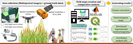
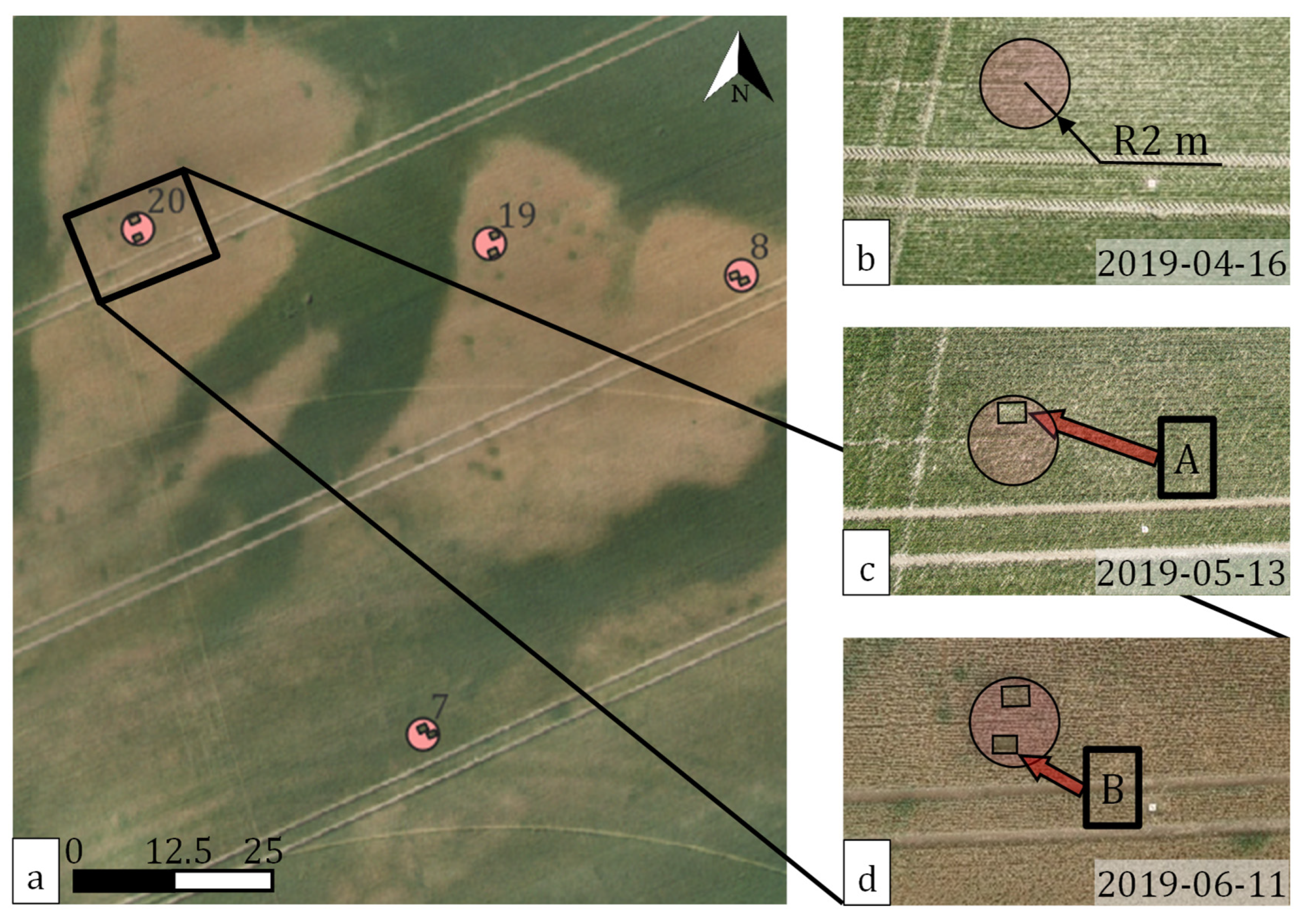
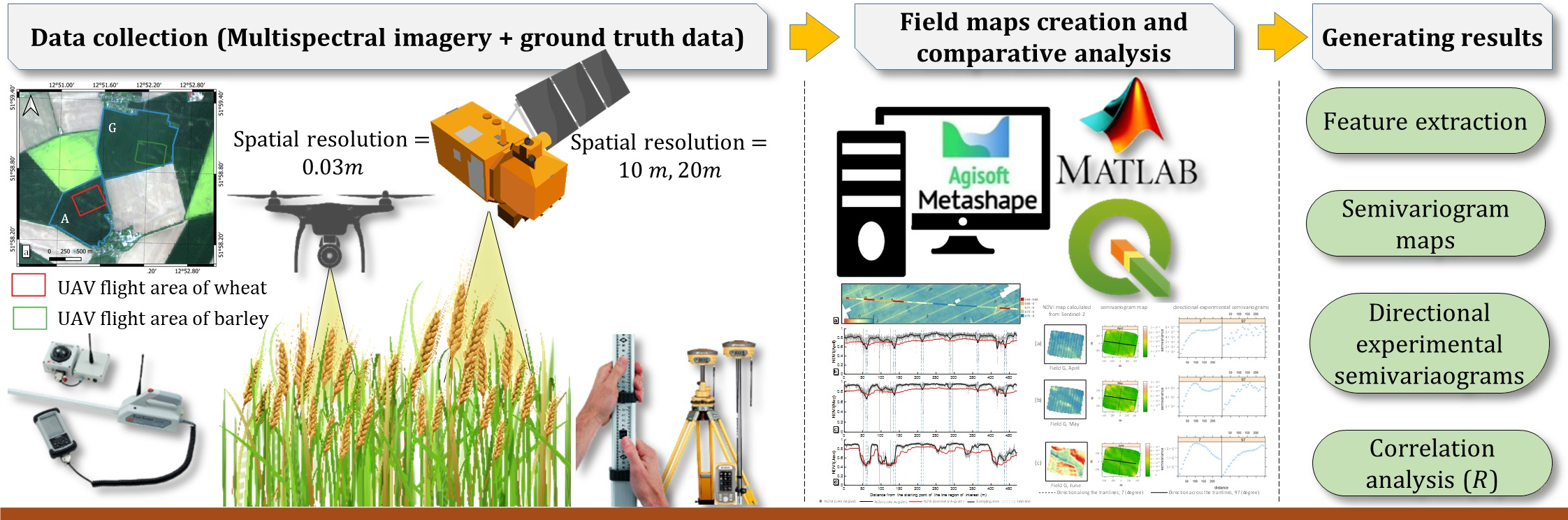
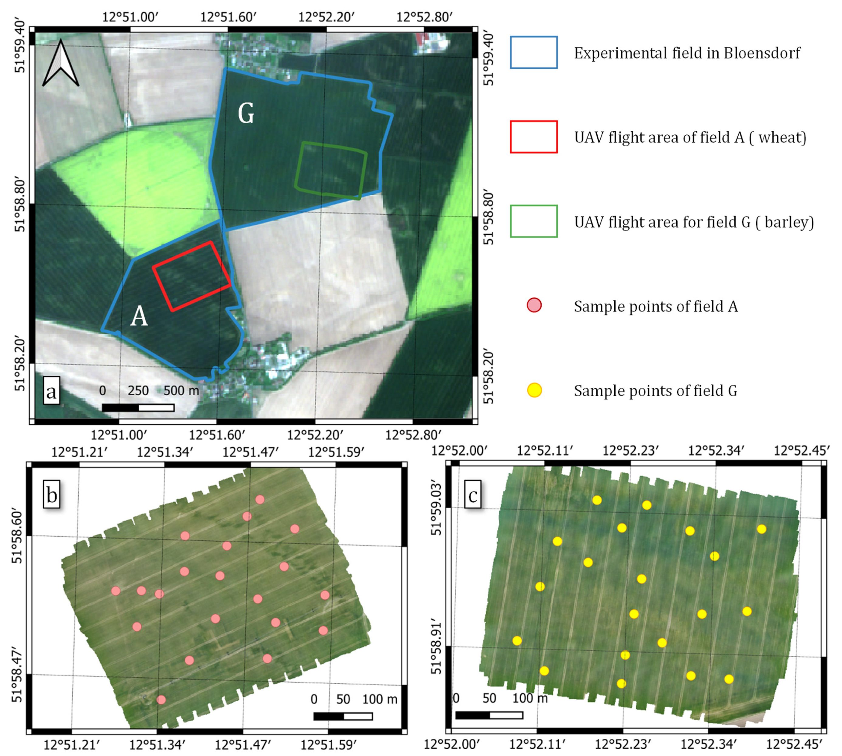
2.1. Study Site and Experimental Field Layout

The study was conducted within two crop fields located near Bloensdorf, Brandenburg, Germany (Lat: 51°58′43.8″N Lon: 12°51′36.1″E) between April and August of 2019 (Figure 1a). The crop types of the experimental sites were wheat and barley, which were labeled as fields A and G, subsequently. The fields were characterized by gentle rolling hills with differences in elevation between 164 and 176 m in field A and 149 and 159 m in field G. The soil development was influenced by late glacial to early Holocene sediments [32]. The soil texture varies between sandy, silty loam, and weak loamy sand. In each field, a rectangle area of 300 m × 400 m was chosen as experimental sites to conduct the comparison between Sentinel-2 and UAV data.

2.2. Reference Data

The experimental sites for field A and field G are shown in Figure 1b,c. Within these areas, 20 sample points for reference measurements were located for each field with respect to the crop variability observed in the previous historical satellite imagery and with respect to an even-distributed spatial coverage. Furthermore, the sample points were also selected with at least a 2 m distance from the tractor lane. At each sample point, the ground area for sampling was spanned by a 2-m-circle in diameters, and plant maximum height, plant mean height, LAI, leaf nitrogen, and fresh biomass (FBM) were determined within its boundaries. Measurements of plant maximum height were recorded by the visible maximum height using a folding yardstick at the location where the fresh biomass was cut. LAI was measured within the sample areas using SunScan Canopy Analysis System type SS1 (Delta-T Devices, Cambridge, UK). The LAI measurement was taken as an average of 10 individual measurements with the probe repositioned each time within the sample area. Leaf nitrogen was measured as an average of 10 individual recordings with the N-pen sensor (Photon Systems Instruments, Drasov, Czech Republic). The handheld device measures the absorption of transmitted light through the plant leaf at green and red wavelengths (595 and 760 nm) due to photosynthesis and characterizes the leaf nitrogen content. For fresh biomass measurement, all wheat and barley plants within the sample area were cut directly above the ground using a handheld electric grass shear within an area of 5 rows by 1 m (approx. 0.75 m2). Cut plants were recorded as fresh biomass by weighing them immediately in the field. Prior to the calculation of VIs, the cut areas for biomass were subtracted from the buffers of sample areas for both UAV and Sentinel-2 imagery according to the actual locations (Section 2.4). Sample points were located using a differential GNSS HiPer Pro system (Topcon Positioning Systems, Inc., Livermore, CA, USA), having a relative horizontal and vertical accuracy of 3 mm and 5 mm. Wheat and barley plant were classified according to the BBCH growth stage code [33] (Section 2.3). The descriptive statistics of the field-measured plant variables used in this paper were summarized in Supplementary Materials Tables S1 and S2.

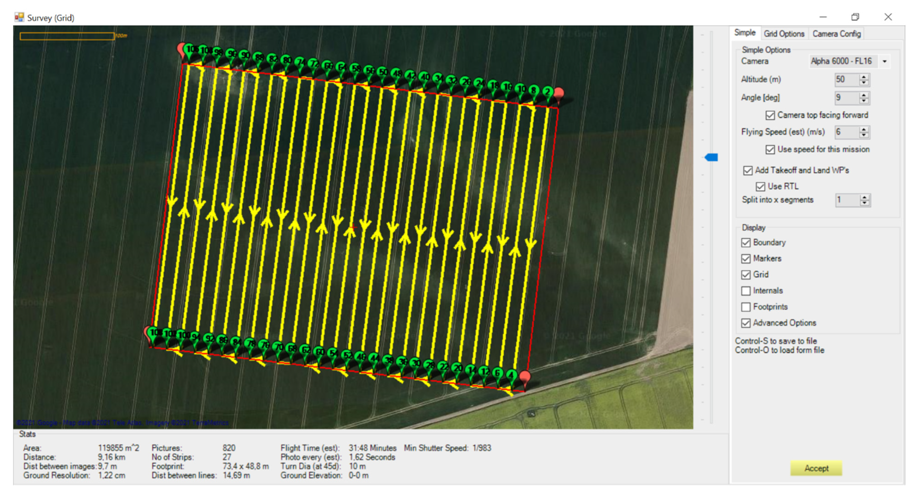
2.3. Remote Sensing Data Acquisition

A multi-rotor UAV model HP-X4-E1200 (HEXAPILOTS, Dresden, Germany) was equipped with a 2-axis gimbal and assembled with a MicaSense RedEdge-M multispectral camera together as the UAV camera platform shown in Figure 2. This platform was used to acquire multispectral images on three different dates during the growing season in fields A and G (Section 2.3) [34]. The multi-spectral camera was a fixed lens system, which provided a field-of-view equivalent to a 5.4 mm focal length (47.2° horizontal, 35.4° vertical field of view). The camera was mounted on the gimbal to provide a nadir view (θ = 0°). During the image acquisition, the camera configuration mode was set to auto-capture mode, which allowed one image capture per second including all spectral bands. Images were recorded with a forward and side overlap of 80% to meet the requirement for structure from motion photogrammetry. As an example, the actual flight route of the UAV for the barley field is shown in Figure 3. The camera technical specification used is listed in Table 1.
The details of the three UAV flight campaigns are summarized in Table 2. Each flight task was labeled as Ai or Gi, where i is the index of the flight task performed on a specific date. The growth stages, BBCH scale, the number of images collected during each flight, wind conditions, satellite imagery acquisition date, and ground measurement dates are also given in Table 2. A total of 11,178 multi-spectral images were collected from all flight tasks at different wind speeds under clear sky conditions over three different growth stages. The back-and-forth flight lines had a distance to each other of 14.69 m to cover the flight area. The UAV was programmed to fly with a ground speed of approximately 6 ms-1 at 50 m height. It resulted in a ground sampling distance (GSD) of approximately 3 cm for the multispectral images. One flight task was composed of five sub-flight tasks due to the battery endurance, and the flight plan was therefore split into five separate flight routes. The flight duration to complete image acquisition for each flight task was approximately between 77 min and 101 min. Ten panels were laid out along a regular grid within the flight areas along the tractor lanes with good visibility from above before the flight campaigns as ground control points (GCPs) and were located by differential GNSS.
Sentinel-2 imagery was acquired on 9 April 2019, 12 May 2019, 11 June, and 13 June 2019 chosen as closely as possible to the dates of UAV flights and ground truth data collection. As shown in Table 1, Sentinel-2 data has 13 bands ranging from 10 to 60-m resolution. The blue (B2), green (B3), red (B4), and near infrared (B8) channels have a 10-m resolution. To match the spectra of the Sentinel-2 with those of the RedEdge camera, the band B2-B4, B5, and B8 were used for analysis in this study.
Sentinel-2 images were first carried out with the atmospheric correction and geo-rectification known as Level-2A collections. These ortho-images were downloaded with the open-source software Quantum GIS 3.22.5 (QGIS) [35] plugin “Semi-Automatic-Classification” [36] with a selected bandset and clipped by a field vector file.
Orthorectification and mosaicking of UAV imagery collections for the different flight campaigns were carried out using the Agisoft Metashape software (Agisoft LLC, St. Petersburg, Russia). Along with the SfM-based photogrammetric workflow embedded in Metashape, high-density point clouds were created. Then, the orthomosaic images were generated from the point cloud-based digital elevation models (DEMs). The GCPs and the MicaSense Calibrated Reflectance Panel (CRP) for the RedEdge camera were used within the processing workflow of the software to generate UAV multispectral orthomosaics with precise scale and position registered to the ETRS 89 UTM Zone 33N coordinate system. Sentinel-2 images were co-registered and georeferenced to the UAV orthomosaic through selected landmark points taken from field and road intersections within the GIS to achieve a consistent multi-temporal data set.

2.4. Data Statistical Analysis

To visualize the spatial variability in the field, seven VIs with five VNIR bands of UAV and Sentinel-2 were chosen for crop monitoring from the literature (Table 3). As the RedEdge band, Sentinel-2 band 5 was chosen for calculating the RedEdge-based VIs.
The extraction of the VI values of the sample areas from both the UAV and Sentinel-2 images was conducted by using a buffer zone generated in QGIS (Figure 4). For each sample, a portion of the above-ground biomass (AGB) is extracted around the center of the sampling area described in Section 2.2. The AGB collection area in the sampling area will affect the subsequent analysis if it is not taken into account and removed. In this case, the buffer zones used in May (Figure 4c) and June (Figure 4a,d) were subtracted by the collection zones for AGB in April and/or May. In the subsequent analysis, the buffer zone was applied to the satellite and UAV images to maintain the consistency of the feature extraction. The different buffer zones of June can be seen in Figure 4a. Finally, the averaged value of the pixel values within the buffer zone was used for calculating the VI values.
We assumed that the management activities have a direct influence on the spatial data because in CTF all management activities are conducted in one direction. To evaluate if directional features are present due to management activities in the spatial data of the NDVI maps, we employed geostatistical analysis tools and investigate this in the context of directional experimental semivariograms and semivariogram maps. They were used to describe the presence, expansion, and compounding of the spatial structure in one or more directions. The directional semivariograms were calculated along and orthogonal to the tramline direction with an angular interval of 10 degrees. Semivariogram values were calculated after removing the first-order trends with OLS regression.
To get a closer look at the differences between UAV and Sentinel-2 imagery, a transect line was created for each field in this study. Each line was located to pass through 3 to 4 sample points to include reference data information. The lines further pass multiple tramlines in the field. We extracted the original NDVI pixel values of the UAV and Sentinel-2 images and applied a moving average filter on the values of UAV and Sentinel-2 to compare them at different growth stages.
Pearson correlation [43] coefficients were calculated for the different VIs in relation to the biophysical reference data at the sample points for the UAV and Sentinel-2 imagery. The r of the Pearson correlation coefficient is calculated.

3. Results

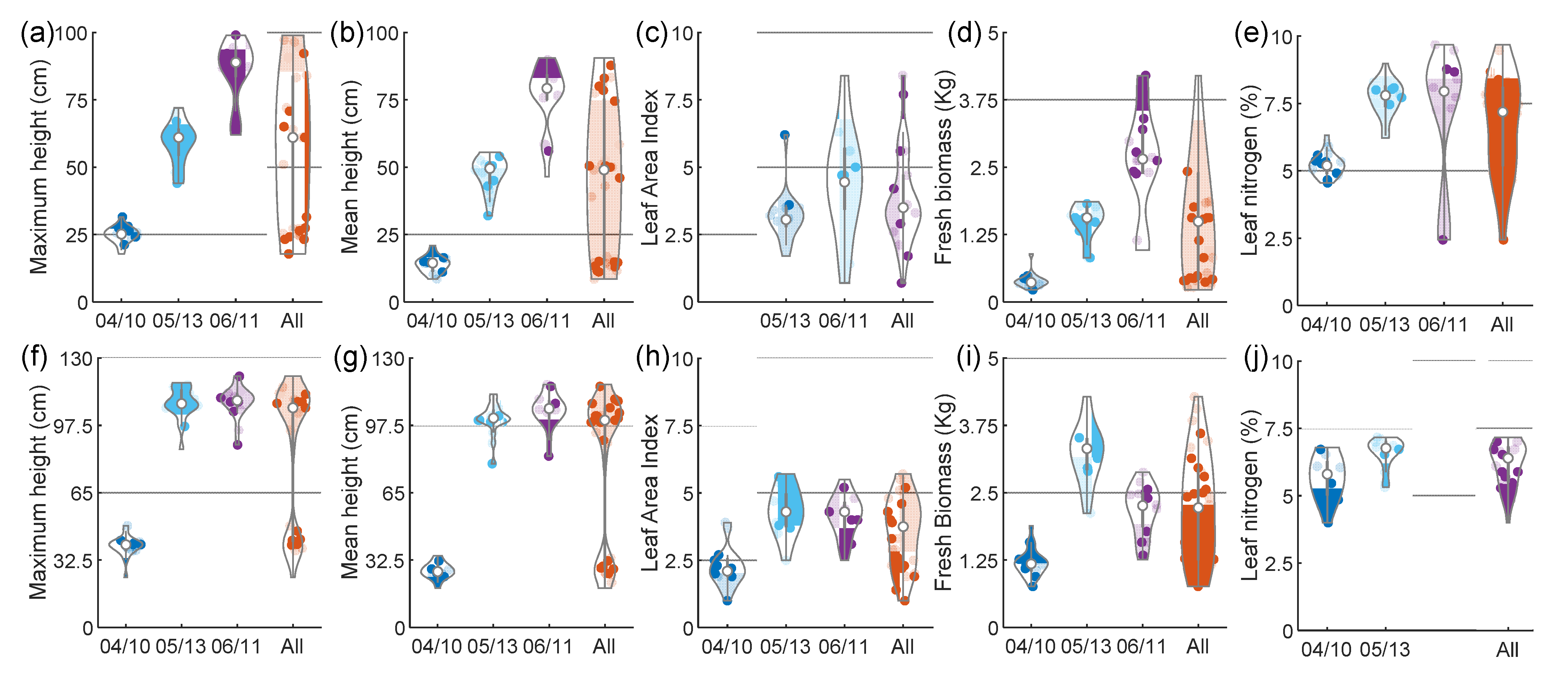
3.1. Distribution of Plant Biophysical and Biochemical Parameters

The distributions of the UAV and Sentinel-2 derived VIs were displayed as violin plots in Figure 5 with data for each growth stage or pooled over the entire season. Three phases of growth stages were observed in both fields during the measurement period. The wheat crop of field A went through tillering (BBCH 23), stem elongation (BBCH 32–33), and fruit development (BBCH 73–77), and the barley crop of field G went through stem elongation (BBCH 31), flowering (BBCH 61–65) and ripening (BBCH 85–89) on the measurement dates in April, May, and June, respectively. Thus, there was a slight difference in crop development between field A and field G, in which the wheat crop grew slower and was harvested later than the barley crop.
Crop height measurements (maximum height and mean height) of wheat were highly variable with a strong increase from growth stage to growth stage (Figure 5a,b), whereas, for barley, the crop height measurements did not show much change or variability from May to June anymore, mainly due to the fact that barley had already flowered in May (Figure 5f,g). In addition, the ears of barley develop long awns, which are not present in wheat. By the time the barley flowered, the ears had already begun to twist downward, while the wheat ears had remained straight until senescence, curling only partially. This difference also affected the expression of the parameter LAI and fresh biomass in both fields. LAI for wheat ranged considerably within each growth stage, especially in June, while the range interval was much greater and in a higher value range than for barley (Figure 5d,i). Fresh biomass of wheat increased between each growth stage and demonstrated the widest value ranges in June, while fresh biomass of barley was highest with the widest value range in May. Due to the differences in crop development, the barley crop was already in the ripening growth stage and senescence was greatly affecting parts of the field compared to wheat, which was still in the fruit development with less senescence. The difference in LAI may also relate to the difference in the growth habitus, where the wheat crop develops a more compact canopy than barley. Leaf N were gradually increased and then started to decrease for both wheat and barley due to the gradual ripening of crop (Figure 5e,j). This is shown by the height of wheat, which appeared to decline slightly. Both varieties have similar growth patterns [44], while wheat and barley are distinguished by their different plant ears. Other differences may be due to a number of factors, including variations in the respective growth stages, soil conditions, and water availability. In general, wheat had a higher leaf density in the canopy than barley.

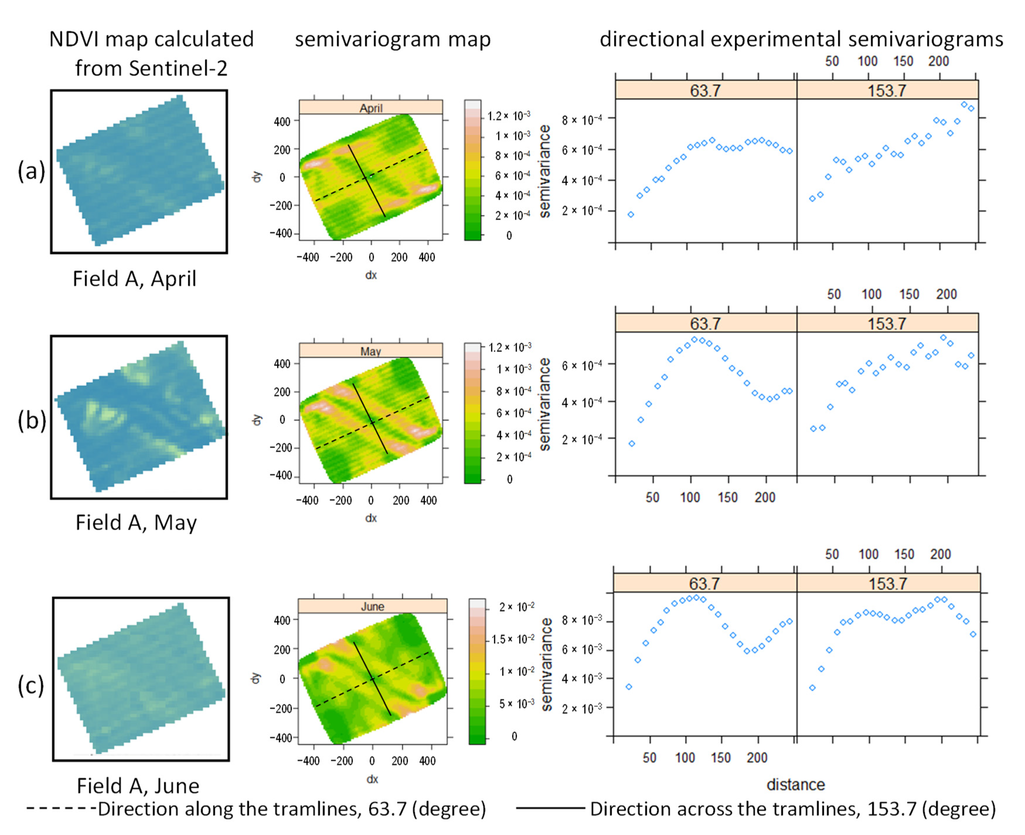
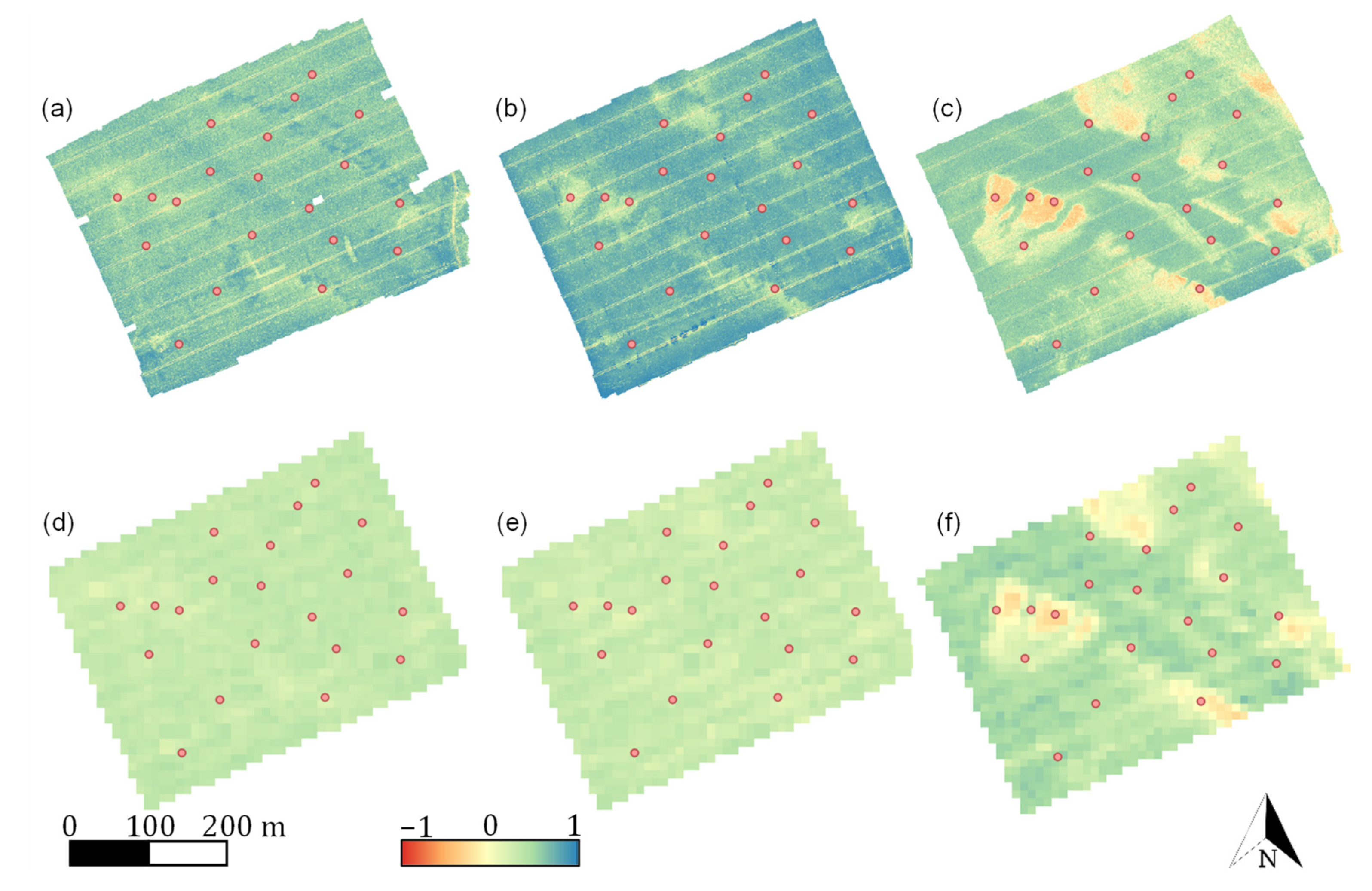
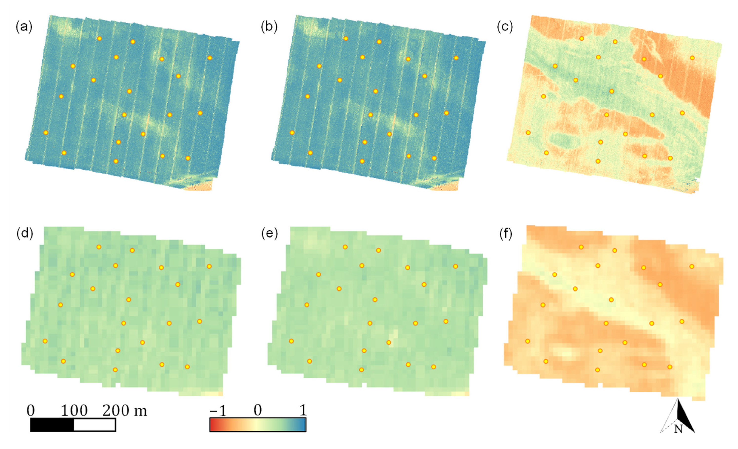
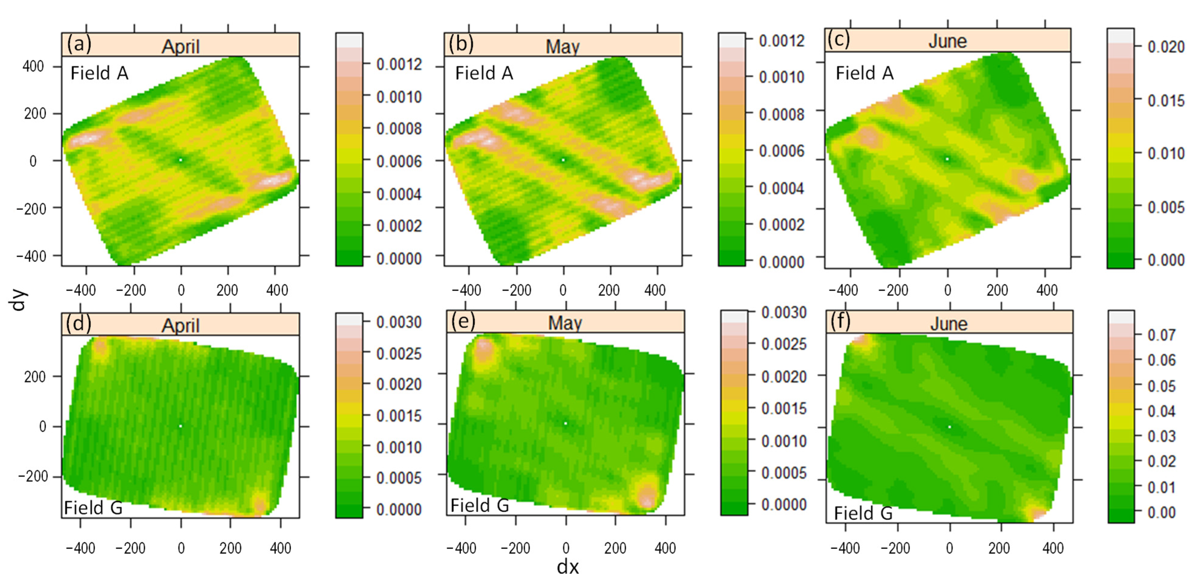
3.2. Spatial Structure and Variability in the UAV and Sentinel-2 Imagery

The vegetative spatial variability of the study sites (A and G) in terms of the Modified Green Red Vegetation Index (MGRVI) maps are presented in Figure 6 and Figure 7 for the UAV and Sentinel-2 imagery of April, May, and June. From a visual inspection of the MGRVI maps (Figure 6 and Figure 7), both UAV and Sentinel-2 follow the same trend over time for each field as reported for example by Nonni et al. [45]. The spatial variation of both fields is strongly characterized by the effects of a former riverbed. In both fields, small, low-growth zones on either side of the old riverbed were caused by gentle slopes and soils with weaker loamy sand that favored water loss through rapid drainage and increased surface water runoff. Within the riverbed, plant growth was better because the soil contained more silt, which improved the water availability for the plants. This soil and the geomorphologic difference were particularly evident in June, where senescence was most pronounced at sites with lower supply (Figure 6c). Outside the river influenced part on the plateaus, plant growth was better than on the slopes but did not reach the optimum as in the riverbed area. In the case of field A, a few exceptions of low-growth areas were located on the plateau. These were caused by insufficient coverage of the irrigation system.
Clearly, the advantage of the UAV imagery over the Sentinel-2 imagery is that even fine spatial details of the canopy structure can be observed in the maps for field-scale assessment (Figure 6 and Figure 7). Yet, despite the lack of details caused by the worse spatial resolution, Sentinel-2 still provides a similar spatial pattern of plant growth for each date comparable to the UAV imagery. Statistically, the MGRVI values derived from Sentinel-2 data were lower than those from the UAV data.
One concern for the study was whether the linear distributed patterns in the Sentinel-2 imagery are associated with management activities. The fields were managed over the season by controlled traffic farming (CTF), which leaves cross-field tramlines. The UAV imagery has a spatial resolution, which was capable of outlining these tramline trajectories accurately in the fields. Interestingly, linear patterns aligned to the tramline direction were also visible in the Sentinel-2 imagery. Thus, it seems that controlled traffic farming in the fields also induces a systematic variation in the Sentinel-2 crop field images. To address this issue from a geostatistics perspective, semivariogram maps and directional experimental semivariograms were generated based on the calculated NDVI from Sentinel-2 images. In Figure 8, the semivariogram maps were shown for the three dates and field A and G, respectively.
The semivariogram maps visualize the spatial dissimilarity in terms of the semivariances along the integrated directions and spatial scales of the fields. Even though the satellite maps have a different distribution of VIs among different growth stages, it is possible to see some similarities in the distribution of tramlines within the crop fields as shown for example clearer visibility for the pattern in the early stage within the semivariogram maps. For April and May, maximum semivariances were approx. 0.0012 and 0.0030 for fields A and G, respectively, which was a magnitude lower than for June when semivariances of 0.020 and 0.07 were reached. For April and May, a strong anisotropy with linear morphological features was present along the tramline direction. They showed a periodicity along the direction of minimum spatial correlation. Furthermore, in both fields, the semivariogram maps had a strong natural pattern superimposing the periodic pattern, which was caused by the soil-induced variability observed in the crop canopies as seen in the MGRVI maps above. In June, the periodic pattern disappeared and the natural pattern became more apparent in the semivariogram maps as crops outgrew the tramlines.
In Figure 9, directional experimental semivariograms are shown calculated with a small angle interval (10°) in the direction of the tramlines and orthogonal to the tramlines for Sentinel-2 NDVI. Basically, the same spatial structure within distances up to 100 m can be seen for the semivariograms from April to June. This structure is strongly governed by the old river-basin pattern and its effects on plant growth. With longer distances semivariances became after a strong rise lower showing a so-called hole effect in the semivariogram, which was markedly stronger expressed for May and June. A hole effect develops in the semivariogram when within larger distances suddenly the points in a spatial field become again more similar due to a repetitive pattern. The similarity of the VI values within longer distances increases due to the effect of the opposite slopes on the crop growth. Another feature can be seen in the directional semivariogram, which was caused by the tramlines. Due to the small bandwidth of the search area in which the semivariances were calculated, the directional semivariograms are generally prone to sudden changes in the spatial pattern of the field. While little fluctuation for the semivariograms calculated along the tramline direction was present, the semivariograms across the tramline direction showed strong fluctuations from lag to lag for April and May. Also, there is a higher semivariance at short distances indicating a possible higher nugget effect for the variogram. This can be explained by the repetitive pattern created by the tramlines in the spatial field because when pixel point pairs of the Sentinel-2 VI images fall within two separated tramlines they bear a subtle higher similarity to each other than for outside point pair comparisons. Thus, the semivariances become slightly lower for those lags, which generates a gentle fluctuation in the directional semivariogram across the tramlines. For June, the fluctuation does not exist anymore because the tramlines were barely existing in the images due to the stronger wheat growth. The same aspects can also be observed for Field G in Figure 10. Again, a hole effect with stronger expression in May and June was generated in the semivariograms due to the natural background effect of the river bed. In addition, semivariograms calculated across the tramline direction had fluctuating semivariances from lag to lag in April and May, with an even greater extent than in Field A.

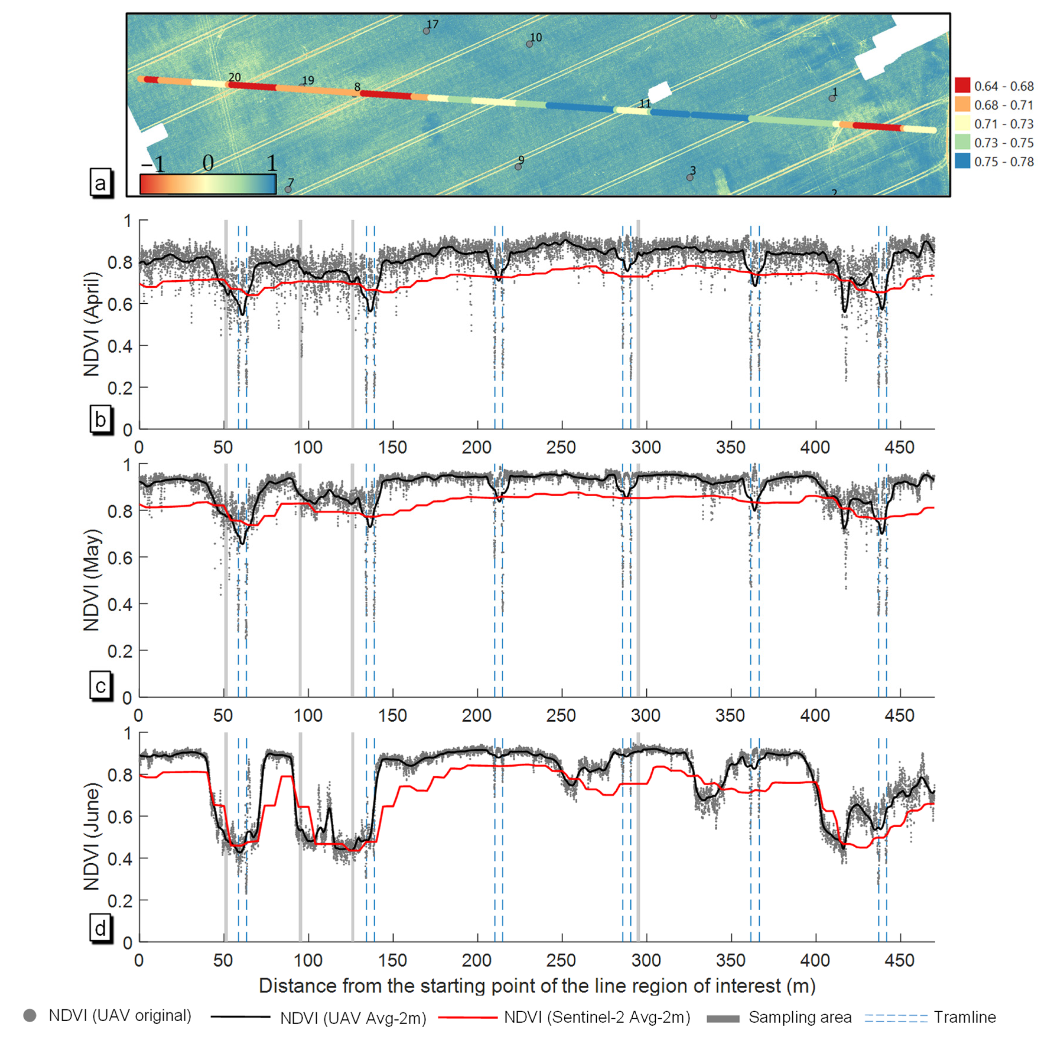
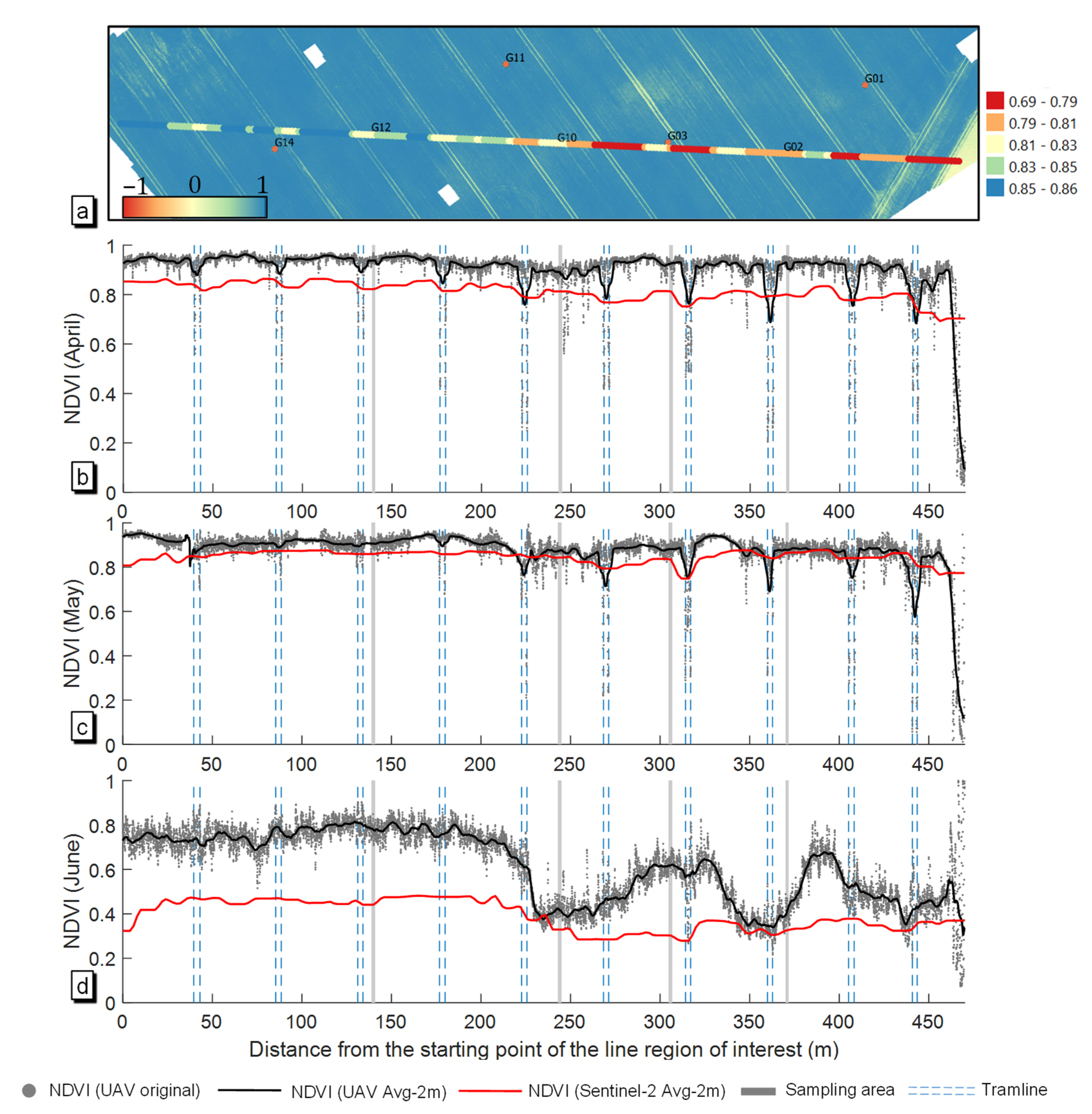
3.3. Comparison of UAV and Sentinel-2 Data along Transect Lines

In Figure 11 and Figure 12, UAV and Sentinel-2 images were compared directly using a transect line representation. In these diagrams, NDVI values were shown along the transect as moving averages extracted from the UAV and Sentinel-2 images and as raw data taken from the UAV in original resolution. The transect line in field A was chosen to cross six tramline pairs and four sampling areas (8, 11, 19, and 20) (Figure 11a). As can be seen from the original UAV NDVI values along the transect line, the data distribution is influenced by the canopy coverage captured during different growth stages. In April, the NDVI values were on average at 0.80, whereas they increased in May to 0.90, and decreased in June to 0.77. This is due to the canopy closure in May as well as stronger absorption of light in the canopy by photosynthesis (peak NDVI). In June, the maximum values were still the same as in May, but strong declines occurred in areas where plants were already in senescence. Furthermore, NDVI values in April showed a larger fluctuation range in a relatively short distance and were more dispersed (Figure 11b), while the data in May and June showed a smaller fluctuation range and presents less variability around the mean value (Figure 11c,d). In April, the variation among the NDVI values around the moving average line was on average 0.056, and for May and June 0.031 and 0.027, respectively. During the tillering growth stage, the canopy was not fully covering the crop area as corroborated by the lower measured LAI values, so that the captured imagery still was influenced by bare soil surface reflection. The strongest decreases in NDVI values were seen at the tramline locations where the soil was strongly exposed. This was also observed to a lesser extent in May. The effect of the tramlines was even stronger in the 2 m down sampled UAV data. Here, the decline started near the tramline pairs, reached a minimum in the middle of the tramline pairs, and then raised back up until it returned to the center of the original value range. This shows that the spacing of tramlines and the diameter of the buffer strongly affects the moving average values of NDVI from UAV imagery, which needs to be taken into account when down sampling the imagery. The original resolution of the UAV images was even high enough that older tramlines from the previous year and seeding errors could be recognized in the NDVI values after rechecking with field observations. In June, the tramlines were nearly overgrown, and the influences of bare soil reflectance due to management activities were strongly reduced. Only small decreases in the NDVI values were observed at the tramline locations along the transect line. In comparison to the NDVI of the UAV images, the NDVI of the Sentinel-2 images had a much smoother outline along the transect line due to the lower spatial resolution of the sensor. It followed on average the UAV transect line but was represented by lower values. In April, even the tramlines had an influence on the distribution of the Sentinel-2 NDVI data, and small decreases in NDVI were recognized at the tramline locations.
The transect line in field G was located through 10 tramline pairs and four sampling areas (2, 3, 10, 12) (Figure 12a). In April, the NDVI values from UAV taken from the original resolution were on average at 0.90, whereas they maintained a similar level of 0.87 in May and dropped sharply to 0.62 in June. This is due to the canopy closure that has been reached in May as well as the strong absorption of light in the canopy by photosynthesis during flowering (peak NDVI). In June, NDVI maximum declined due to the stronger maturity across the field and the greatest decline occurred in areas where plants were already in senescence. Furthermore, NDVI values in April were more concentrated and showed the smallest fluctuation range (Figure 12b). The fluctuation range in May increased slightly (Figure 12c), while the data in June showed the largest fluctuation range (Figure 12d). In April and May, the variation among the NDVI values around the moving average line was on average 0.031 and 0.034, and for June 0.040, respectively. This might be because during the stem elongation and flowering stages, the canopy was fully covering the crop areas as corroborated by the small deviation from the measured LAI values, so that the ortho-image generated by the UAV captured images contains fewer soil components, and the captured imagery was mostly influenced by light absorption in the canopy. Strong declines of NDVI values occurred at the tramline locations where the soil was strongly exposed to the sensors (Figure 12c,d), which was observed to a lesser extent than in the wheat field. In June, the tramlines were nearly overgrown in the field, and only little influences of bare soil reflectance were observed due to management activities in field G. It needs to be pointed out that the bent barley spikes in June have influenced the variation of NDVI after rechecking with field observations so that the distribution of NDVI pixels gradually dispersed (Figure 12d). In comparison to the NDVI of the UAV images, the NDVI of the Sentinel-2 images also shows a smoother outline representing lower values due to the spatial resolution of the sensor. In April and May, the Sentinel-2 NDVI was also influenced by the tramlines, which caused small decreases of the NDVI values. This indicates that when using Sentinel-2 data as a kind of source data for precision agriculture, the NDVI values are still affected by the agricultural management within the field, and it cannot be eliminated by averaging. Some researchers suggested to reduce the effect of the borders of the field [30]. We suggest that in order to obtain the true value in the crop field through Sentinel-2, it is also necessary to be 10 m away from the tramlines in order to avoid the sentinel-2 data being a mixed pixel of soil and plants within the field.

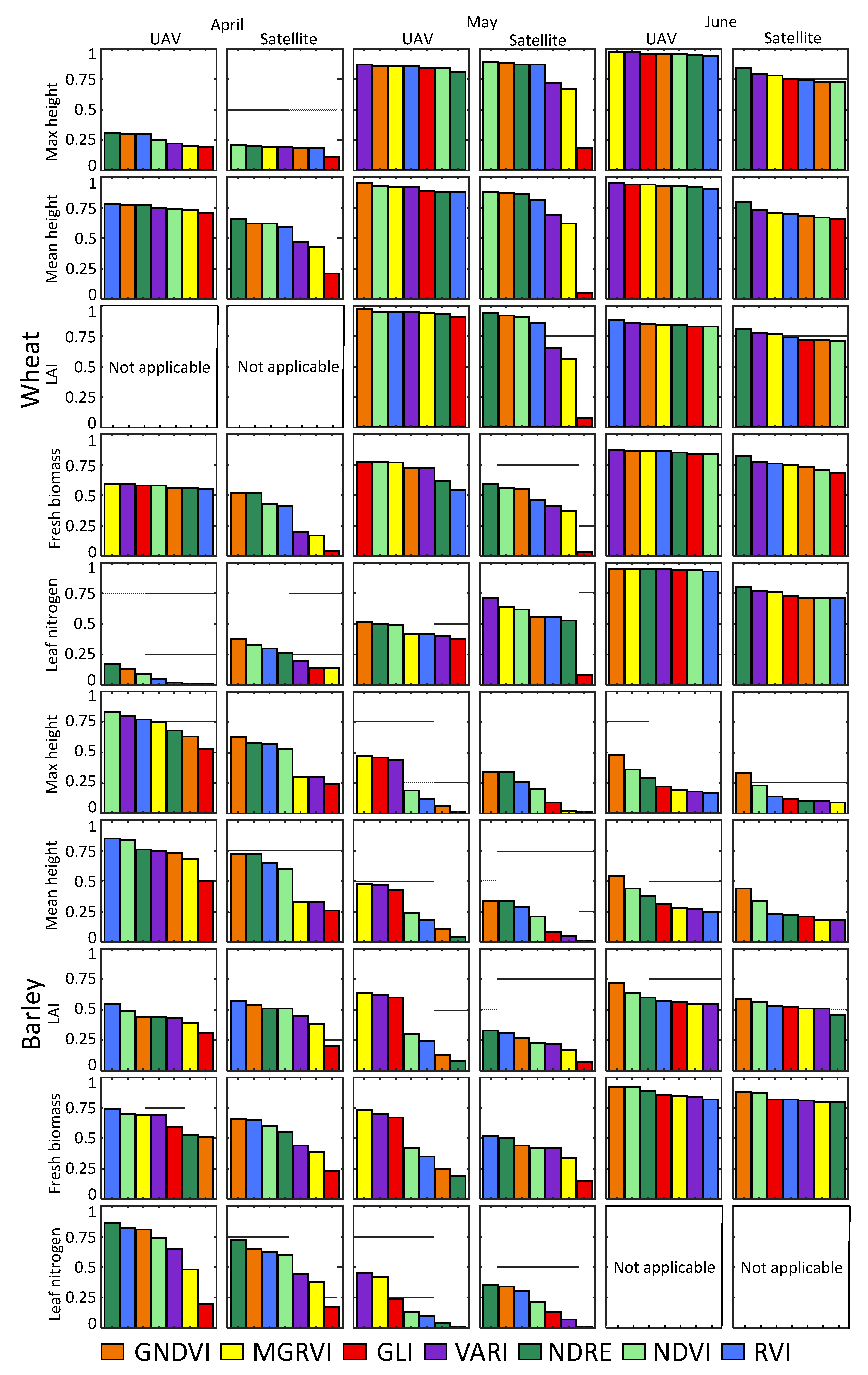
3.4. Correlation of UAV and Sentinel-2 VIs with Agronomic Parameters

In Figure 13, different VIs extracted from the UAV, and Sentinel-2 images were compared with the reference data collected at the sample points with Pearson correlation coefficients. For wheat in field A, no significant correlations were found for both UAV and Sentinel-2 data for maximum plant height and leaf nitrogen in April, whereas for fresh biomass and mean height average correlations were reached with slightly better correlations for UAV. With increasing growth stage, correlation with the reference data increased and was significant in April and May, with the strongest gradual increase for leaf nitrogen. The highest correlation was reached in June for all parameters, except for LAI, which was slightly worse than the correlations found in May. Generally, correlations for Sentinel-2 were slightly worse. In addition, they had a stronger variation among different VI types than compared with the UAV data in April and May. Specifically, GLI, MGRVI, and VARI had the lowest correlation with the reference data in April and May. All three VIs were calculated from bands in the VIS part of the spectrum. In contrast, for UAV, those bands were very well correlated with the reference data in most cases. It seems that the NIR bands are important for Sentinel-2 for relating the data to the agronomic parameters. UAV has its benefits from higher spatial resolution, such as more detailed information from the sensors and accurate positions for the sample areas, which compensate for the drawback of the calculation from the VIS part of the spectrum. Interestingly, however, this was not true for the correlations with leaf nitrogen in May. Here, the VARI from Sentinel-2 performed best, even better than the corresponding VIs calculated from the UAV data.
For barley in field G, higher correlations were obtained in April than compared with the correlation obtained in field G in wheat, probably due to the fact that the plants already have been further in growth within stem elongation. The lowest correlation was found for LAI in April, whereas the other agronomic parameters correlated at the same average level with UAV or Sentinel-2. In May, correlation decreased for most agronomic parameters, except for the correlation of LAI and fresh biomass with UAV data, which slightly improved. In June, the highest correlation in total was found for LAI and fresh biomass, whereas for crop height, the correlations were not significant and due to the effect of senescence, leaf nitrogen was not measurable on the ground. Similarly, UAV data was marginally better related to the agronomic parameters than Sentinel-2 data. The highest difference between UAV and Sentinel-2 was found in May. Here, GLI, MGRVI, and VARI calculated from UAV data correlated exceptionally, well especially for fresh biomass and LAI. In contrast, for Sentinel-2, GLI, MGRVI, and VARI were again the VIs with the worst correlations to the agronomic parameters in April and May. The detailed numbers of the correlation coefficients for plant parameters calculated in this paper were summarized in Supplementary Materials Table S3–S10.

4. Discussion

Crop growers need timely spatial information on the variability of agronomic crop parameters throughout the season so they can make the right management decisions to reduce costs and environmental impact. UAV and Sentinel-2 provide information for the agronomic parameter in crop fields with the VIs, and they are important tools for precision agriculture.
To meet the requirements of modern precision agriculture, especially in the area of crop production, for more detailed information as well as a balanced cost/performance ratio, a comparative study based on Sentinel-2 and UAV delivers interesting new data. The experiments conducted within this framework used the original spatial resolution of Sentinel-2 and UAV imagery. Multispectral data from the Sentinel-2 and UAV-based camera system was used to characterize the agronomic parameters of the crop and were later compared directly using a transect-line representation.
Results are based on data from wheat and barley during the growth season. Two 12 ha fields, including data from flight campaigns of three dates in the season, and the corresponding Sentinel-2 data, were used as a comparative study. The comparison of crop agronomic parameters obtained from the UAV and Sentinel-2 with reference ground truth data showed that the UAV images are suitable for finer observation of crop growth from the canopy structure and non-canopy structure.
The fields were managed over the season by CTF, which leaves permanent cross-field tramlines. Comparing UAV and satellite data in this study, a relatively large error in the Sentinel-2 data was found close to the tramlines. The strongest decreases in pixel values were seen at the tramline locations where the soil was strongly exposed. Also, there was observed reduction to a lesser extent in the Sentinel-2 data. The effect of tramlines influenced not only UAV data but also Sentinel-2 data. Prior research has not found the linear-distributed patterns associated with management activities and that it has a systematic influence on the Sentinel-2 imagery. It would be interesting if the inaccuracy caused by management-driven features in crop fields could be solved if open-source or inexpensive satellite data with 2 m resolution or less were readily available for the farmer, such as Planet or Worldwide-2 imagery.
Some limitations in the study arise from the fact that the Sentinel-2 and the UAV images were acquired with a time lag of one to seven days because the flight campaign for the UAV data acquisition was planned according to the actual weather situation. This time difference cannot be compensated for and may lead to some uncertainty.

5. Conclusions

Sentinel-2 and multispectral UAV imagery were comparatively analyzed to characterize biophysical plant parameters and leaf nitrogen of wheat and barley crops from a practical perspective close to agricultural routines. The target beneficiary audience for this study is crop growers using precision agriculture approaches and data providers of remote sensing services. The investigation and statistical analysis of UAV and Sentinel-2 for two field areas regarding the spatial variability observed within the fields over three months led to the following remarks:
  • In general, they both follow the same large-scale pattern when the differences in the pattern were well expressed, e.g., the effect of the large river-bed on plant growth over the season was recognizable with UAV and with Sentinel-2 imagery.
  • Management-related features can have an influence on the Sentinel-2 imagery in specific cases. The slim tramlines of CTF often used in German agriculture, have a systematic influence on the Sentinel-2 images. This was observed in the spatial pattern as well as in the semivariograms calculated from the Sentinel-2 images in this study. However, Sentinel-2 does not have enough spatial accuracy to accurately delineate the tramline positions.
  • UAV data slightly outperforms Sentinel-2 data in their relationship to agronomic parameters, but rarely does the UAV correlation greatly exceed that over Sentinel-2 data. There was, however, a strong variation in the correlation among different VIs when Sentinel-2 was used to calculate them, and our study suggests that VIs solely built from VIS bands should not be considered for relating to agronomic parameters, at least not for the biophysical parameters LAI, biomass, and crop height. In contrast, the correlation of VIs from UAV data was not affected and strongly varied by different VIs.
In conclusion, we would recommend the use of UAV data to meet the requirements for more detailed information in modern precision agriculture. The choice of the most appropriate technology or combination strategy depends on the aim of the collection, as they have different spatial analyses, requirements, labor, and time cost. We would advise that fusing UAV with Sentinel-2 imagery taken early in the season may help improve crop monitoring and to reduce costs as it can integrate the effect of agricultural management in the subsequent absence of high spatial resolution data. Future research should explore how to make better use of both technologies to reduce management costs and improve agricultural management efficiency.

Supplementary Materials

The following supporting information can be downloaded at: https://www.mdpi.com/article/10.3390/rs14174426/s1, Table S1: Summary statistics of the plant trait variables measured at 20 sample points in field A; Table S2: Summary statistics of the plant trait variables measured at 20 sample points in field G; Table S3: Absolute correlation results of plant maximum height and mean height in field A; Table S4: Absolute correlation results of plant maximum height and mean height in field G; Table S5: Absolute correlation results of LAI in field A; Table S6: Absolute correlation results of LAI in field G; Table S7: Absolute correlation results of fresh biomass in field A; Table S8: Absolute correlation results of fresh biomass in field G; Table S9: Absolute correlation results of leaf nitrogen in field A; Table S10. Absolute correlation results of leaf nitrogen in field G.

Author Contributions

Conceptualization, M.L. and M.S.; methodology, M.L. and M.S.; software, M.L. and M.S.; validation, M.L., M.S. and R.R.S.; formal analysis, M.L. and M.S.; investigation, C.W.; resources, C.W.; data curation, M.L.; writing—original draft preparation, M.L. and M.S.; writing—review and editing, M.L., M.S. and R.R.S.; visualization, M.L.; supervision, C.W. and M.S.; project administration, C.W.; funding acquisition, C.W. and M.L. All authors have read and agreed to the published version of the manuscript.

Funding

This research received no external funding.

Data Availability Statement

Data is contained within the article.

Acknowledgments

The authors would like to acknowledge the support from the China Scholarship Council (CSC), the Leibniz Institute for Agricultural Engineering and Bioeconomy (ATB), and Technische Universität Berlin (TU Berlin). A sincere thank you goes to Katharina Harfenmeister from (GFZ) who helped us with the communication with farmer and provided valuable insights into this study. The fieldworks and data collection support from Antje Giebel, Franziska Gleiniger, and Marc Zimne are duly acknowledged.

Conflicts of Interest

The authors declare no conflict of interest.

References

  1. Sudduth, K.A.; Hummel, J.W.; Birrell, S.J. Sensors for Site-Specific Management. In The State of Site Specific Management for Agriculture; American Society of Agronomy: Madison, WI, USA, 1997; pp. 183–210. [Google Scholar]
  2. Gebbers, R.; Adamchuk, V.I. Precision Agriculture and Food Security. Science 2010, 327, 828–831. [Google Scholar] [CrossRef]
  3. Jones, J.W.; Antle, J.M.; Basso, B.; Boote, K.J.; Conant, R.T.; Foster, I.; Godfray, H.C.J.; Herrero, M.; Howitt, R.E.; Janssen, S.; et al. Brief History of Agricultural Systems Modeling. Agric. Syst. 2017, 155, 240–254. [Google Scholar] [CrossRef]
  4. Diacono, M.; Rubino, P.; Montemurro, F. Precision Nitrogen Management of Wheat. A Review. Agron. Sustain. Dev. 2013, 33, 219–241. [Google Scholar] [CrossRef]
  5. FAO. Sampling Methods for Agricultural Surveys; FAO: Rome, Italy, 1989. [Google Scholar]
  6. Bosecker, R.R. Sampling Methods in Agriculture; National Agricultural Statistics Service, US Department of Agriculture: Washington, DC, USA, 1988. [Google Scholar]
  7. Ziliani, M.G.; Parkes, S.D.; Hoteit, I.; McCabe, M.F. Intra-Season Crop Height Variability at Commercial Farm Scales Using a Fixed-Wing UAV. Remote Sens. 2018, 10, 2007. [Google Scholar] [CrossRef]
  8. Comba, L.; Biglia, A.; Ricauda Aimonino, D.; Tortia, C.; Mania, E.; Guidoni, S.; Gay, P. Leaf Area Index Evaluation in Vineyards Using 3D Point Clouds from UAV Imagery. Precis. Agric. 2020, 21, 881–896. [Google Scholar] [CrossRef]
  9. Ten Harkel, J.; Bartholomeus, H.; Kooistra, L. Biomass and Crop Height Estimation of Different Crops Using UAV-Based LiDAR. Remote Sens. 2020, 12, 17. [Google Scholar] [CrossRef]
  10. Campos-Taberner, M.; García-Haro, F.J.; Busetto, L.; Ranghetti, L.; Martínez, B.; Gilabert, M.A.; Camps-Valls, G.; Camacho, F.; Boschetti, M. A Critical Comparison of Remote Sensing Leaf Area Index Estimates over Rice-Cultivated Areas: From Sentinel-2 and Landsat-7/8 to MODIS, GEOV1 and EUMETSAT Polar System. Remote Sens. 2018, 10, 763. [Google Scholar] [CrossRef]
  11. Berger, K.; Verrelst, J.; Féret, J.-B.; Wang, Z.; Wocher, M.; Strathmann, M.; Danner, M.; Mauser, W.; Hank, T. Crop Nitrogen Monitoring: Recent Progress and Principal Developments in the Context of Imaging Spectroscopy Missions. Remote Sens. Environ. 2020, 242, 111758. [Google Scholar] [CrossRef]
  12. Poley, L.G.; McDermid, G.J. A Systematic Review of the Factors Influencing the Estimation of Vegetation Aboveground Biomass Using Unmanned Aerial Systems. Remote Sens. 2020, 12, 1052. [Google Scholar] [CrossRef]
  13. Zecha, C.W.; Link, J.; Claupein, W. Mobile Sensor Platforms: Categorisation and Research Applications in Precision Farming. J. Sens. Sens. Syst. 2013, 2, 51–72. [Google Scholar] [CrossRef] [Green Version]
  14. Bogue, R. Sensors Key to Advances in Precision Agriculture. Sens. Rev. 2017, 37, 1–6. [Google Scholar] [CrossRef]
  15. Zhang, L.; Zhang, H.; Niu, Y.; Han, W. Mapping Maize Water Stress Based on UAV Multispectral Remote Sensing. Remote Sens. 2019, 11, 605. [Google Scholar] [CrossRef]
  16. Shendryk, Y.; Sofonia, J.; Garrard, R.; Rist, Y.; Skocaj, D.; Thorburn, P. Fine-Scale Prediction of Biomass and Leaf Nitrogen Content in Sugarcane Using UAV LiDAR and Multispectral Imaging. Int. J. Appl. Earth Obs. Geoinf. 2020, 92, 102177. [Google Scholar] [CrossRef]
  17. Neupane, K.; Baysal-Gurel, F. Automatic Identification and Monitoring of Plant Diseases Using Unmanned Aerial Vehicles: A Review. Remote Sens. 2021, 13, 3841. [Google Scholar] [CrossRef]
  18. Hassan, M.A.; Yang, M.; Rasheed, A.; Yang, G.; Reynolds, M.; Xia, X.; Xiao, Y.; He, Z. A Rapid Monitoring of NDVI across the Wheat Growth Cycle for Grain Yield Prediction Using a Multi-Spectral UAV Platform. Plant Sci. 2019, 282, 95–103. [Google Scholar] [CrossRef]
  19. Walsh, O.S.; Shafian, S.; Marshall, J.M.; Jackson, C.; McClintick-Chess, J.R.; Blanscet, S.M.; Swoboda, K.; Thompson, C.; Belmont, K.M.; Walsh, W.L. Assessment of UAV Based Vegetation Indices for Nitrogen Concentration Estimation in Spring Wheat. Adv. Remote Sens. 2018, 7, 71–90. [Google Scholar] [CrossRef]
  20. Rose, J.C.; Kicherer, A.; Wieland, M.; Klingbeil, L.; Töpfer, R.; Kuhlmann, H. Towards Automated Large-Scale 3D Phenotyping of Vineyards under Field Conditions. Sensors 2016, 16, 2136. [Google Scholar] [CrossRef]
  21. Piragnolo, M.; Lusiani, G.; Pirotti, F. Comparison of Vegetation Indices from RPAS and Sentinel-2 Imagery for Detecting Permanent Pastures. Int. Arch. Photogramm. Remote Sens. Spat. Inf. Sci. 2018, 42, 1381–1387. [Google Scholar] [CrossRef]
  22. Gascon, F.; Cadau, E.; Colin, O.; Hoersch, B.; Isola, C.; Fernández, B.L.; Martimort, P. Copernicus Sentinel-2 Mission: Products, Algorithms and Cal/Val. In Proceedings of the Earth Observing Systems XIX, San Diego, CA, USA, 17–21 August 2014; SPIE: Bellingham, WA, USA, 2014; Volume 9218, pp. 455–463. [Google Scholar]
  23. Drusch, M.; Del Bello, U.; Carlier, S.; Colin, O.; Fernandez, V.; Gascon, F.; Hoersch, B.; Isola, C.; Laberinti, P.; Martimort, P. Sentinel-2: ESA’s Optical High-Resolution Mission for GMES Operational Services. Remote Sens. Environ. 2012, 120, 25–36. [Google Scholar] [CrossRef]
  24. Delloye, C.; Weiss, M.; Defourny, P. Retrieval of the Canopy Chlorophyll Content from Sentinel-2 Spectral Bands to Estimate Nitrogen Uptake in Intensive Winter Wheat Cropping Systems. Remote Sens. Environ. 2018, 216, 245–261. [Google Scholar] [CrossRef]
  25. Revill, A.; Florence, A.; MacArthur, A.; Hoad, S.P.; Rees, R.M.; Williams, M. The Value of Sentinel-2 Spectral Bands for the Assessment of Winter Wheat Growth and Development. Remote Sens. 2019, 11, 2050. [Google Scholar] [CrossRef]
  26. Chamen, T. Controlled Traffic Farming—From Worldwide Research to Adoption in Europe and Its Future Prospects. Acta Technol. Agric. 2015, 18, 64–73. [Google Scholar] [CrossRef]
  27. Su, J.; Liu, C.; Coombes, M.; Hu, X.; Wang, C.; Xu, X.; Li, Q.; Guo, L.; Chen, W.-H. Wheat Yellow Rust Monitoring by Learning from Multispectral UAV Aerial Imagery. Comput. Electron. Agric. 2018, 155, 157–166. [Google Scholar] [CrossRef]
  28. Cohrs, C.W.; Cook, R.L.; Gray, J.M.; Albaugh, T.J. Sentinel-2 Leaf Area Index Estimation for Pine Plantations in the Southeastern United States. Remote Sens. 2020, 12, 1406. [Google Scholar] [CrossRef]
  29. Di Gennaro, S.F.; Dainelli, R.; Palliotti, A.; Toscano, P.; Matese, A. Sentinel-2 Validation for Spatial Variability Assessment in Overhead Trellis System Viticulture Versus UAV and Agronomic Data. Remote Sens. 2019, 11, 2573. [Google Scholar] [CrossRef]
  30. Sozzi, M.; Kayad, A.; Marinello, F.; Taylor, J.; Tisseyre, B. Comparing Vineyard Imagery Acquired from Sentinel-2 and Unmanned Aerial Vehicle (UAV) Platform. Oeno One 2020, 54, 189–197. [Google Scholar] [CrossRef]
  31. Messina, G.; Peña, J.M.; Vizzari, M.; Modica, G. A Comparison of UAV and Satellites Multispectral Imagery in Monitoring Onion Crop. An Application in the ‘Cipolla Rossa Di Tropea’ (Italy). Remote Sens. 2020, 12, 3424. [Google Scholar] [CrossRef]
  32. Nicolay, A. Untersuchungen zur (Prä-)Historischen Relief-, Boden- und Landschaftsentwicklung im Südlichen Brandenburg (Niederlausitz). Ph.D. Thesis, BTU Cottbus, Senftenberg, Germany, 2017. [Google Scholar]
  33. Meier, U. Growth Stages of Mono- and Dicotyledonous Plants: BBCH Monograph; Blackwell Wissenschafts-Verlag: Berlin, Germany; Boston, MA, USA, 1997; ISBN 3826331524/9783826331527. [Google Scholar]
  34. Li, M.; Shamshiri, R.R.; Schirrmann, M.; Weltzien, C.; Shafian, S.; Laursen, M.S. UAV Oblique Imagery with an Adaptive Micro-Terrain Model for Estimation of Leaf Area Index and Height of Maize Canopy from 3D Point Clouds. Remote Sens. 2022, 14, 585. [Google Scholar] [CrossRef]
  35. QGIS Development Team. QGIS Geographic Information System; QGIS Association: Gossau, Switzerland, 2015. [Google Scholar]
  36. Congedo, L. Semi-Automatic Classification Plugin, version 6.0.1.1; ResearchGate: Berlin, Germany, 2016. [Google Scholar] [CrossRef]
  37. Louhaichi, M.; Borman, M.M.; Johnson, D.E. Spatially Located Platform and Aerial Photography for Documentation of Grazing Impacts on Wheat. Geocarto Int. 2001, 16, 65–70. [Google Scholar] [CrossRef]
  38. Gitelson, A.A.; Merzlyak, M.N. Remote Estimation of Chlorophyll Content in Higher Plant Leaves. Int. J. Remote Sens. 1997, 18, 2691–2697. [Google Scholar] [CrossRef]
  39. Bendig, J.; Yu, K.; Aasen, H.; Bolten, A.; Bennertz, S.; Broscheit, J.; Gnyp, M.L.; Bareth, G. Combining UAV-Based Plant Height from Crop Surface Models, Visible, and near Infrared Vegetation Indices for Biomass Monitoring in Barley. Int. J. Appl. Earth Obs. Geoinf. 2015, 39, 79–87. [Google Scholar] [CrossRef]
  40. Rouse, J.W., Jr.; Haas, R.H.; Schell, J.A.; Deering, D.W. Monitoring Vegetation Systems in the Great Plains with Erts. In NASA Special Publication; NASA: Washington, DC, USA, 1974; Volume 351, p. 309. [Google Scholar]
  41. Huete, A.; Didan, K.; Miura, T.; Rodriguez, E.P.; Gao, X.; Ferreira, L.G. Overview of the Radiometric and Biophysical Performance of the MODIS Vegetation Indices. Remote Sens. Environ. 2002, 83, 195–213. [Google Scholar] [CrossRef]
  42. Gitelson, A.A. Wide Dynamic Range Vegetation Index for Remote Quantification of Biophysical Characteristics of Vegetation. J. Plant Physiol. 2004, 161, 165–173. [Google Scholar] [CrossRef]
  43. Benesty, J.; Chen, J.; Huang, Y.; Cohen, I. Pearson Correlation Coefficient. In Noise Reduction in Speech Processing; Springer: Berlin/Heidelberg, Germany, 2009; pp. 1–4. [Google Scholar]
  44. Harfenmeister, K.; Spengler, D. Analyzing Temporal and Spatial Characteristics of Crop Parameters Using Sentinel-1 Backscatter Data. Remote Sens. 2019, 11, 1569. [Google Scholar] [CrossRef]
  45. Nonni, F.; Malacarne, D.; Pappalardo, S.E.; Codato, D.; Meggio, F.; De Marchi, M. Sentinel-2 Data Analysis and Comparison with UAV Multispectral Images for Precision Viticulture. GI Forum 2018, 1, 105–116. [Google Scholar] [CrossRef]
Figure 1. The layout of the study site and the distributions of the flight areas. The (a) study site was marked as blue line. The UAV flight area for field A was marked as red line (b). The UAV flight area for field G was marked as green line (c). The sampling locations of canopy height, LAI, leaf nitrogen were marked as pink dots (field A) and yellow dots (field G). The main soil type is eolian sediments and glacial sediments, and the soil texture varies between sandy, silty loam, and weak loamy sand.
Remotesensing 14 04426 g001
Figure 2. UAV-based imagery acquisition.
Remotesensing 14 04426 g002
Figure 3. The actual flight route of UAV for the barley field.
Remotesensing 14 04426 g003
Figure 4. Illustration of buffer zones used in this study. The June’s buffer zone was marked in pink (a,d). The April buffer consists of a circle with a radius of 2 m (b). Central points are located by GNSS. Because each ground measurement involves sampling of biomass, the (c) May and (d) June buffers need to remove the subtracted biomass area according to the actual location. The squares represent the cut biomass in April and May, which are marked as A and B, respectively.
Remotesensing 14 04426 g004
Figure 5. Comparison of measured parameters from wheat and barley crop. Upper row refers to field A and wheat crop (ae), bottom row refers to field G and barley crop (fj). The violin plot demonstrates the maximum, minimum, median (white point), first, and third quartile (start and end of line) values of the plant parameters, and the width of each violin element represents the frequency of the plant parameters.
Remotesensing 14 04426 g005
Figure 6. Modified green red vegetation index (MGRVI) of the study area A for wheat. UAV imagery was acquired on (a) 16 April 2019, (b) 13 May 2019, and (c) 11 June 2019. Sentinel-2 imagery was acquired on (d) 9 April 2019, (e) 12 May 2019, and (f) 13 June 2019. The points indicate the locations for reference sampling.
Remotesensing 14 04426 g006
Figure 7. Modified green red vegetation index (MGRVI) of the study area G for barley. UAV imagery was acquired on (a) 16 April 2019, (b) 13 May 2019, and (c) 13 June 2019. Sentinel-2 imagery was acquired: on (d) 9 April 2019, (e) 12 May 2019, and (f) 13 June 2019. The points indicate the locations for reference sampling.
Remotesensing 14 04426 g007
Figure 8. Semivariogram maps of NDVI maps calculated based on raw Sentinel-2 data at different growth stages from field A and wheat crop (ac), field G and barley crop (df) in: (a) April 2019, (b) May 2019, and (c) June 2019 of field A, (d) April 2019, (e) May 2019, and (f) June 2019 of field G.
Remotesensing 14 04426 g008
Figure 9. Relationship between the semivariogram map and experimental semivariograms calculated along and across the tramline direction for (a) April, (b) May, and (c) June for field A. From left to right, it shows the NDVI image, the semivariogram map calculated from Sentinel-2 NDVI and profiles of directional experimental semivariograms along and across the tramlines. The dashed and continuous line in the semivariogram maps indicate the direction of the along and across tramline directional semivariograms.
Remotesensing 14 04426 g009
Figure 10. Relationship between the semivariogram map and directional experimental semivariograms calculated along and across the tramline direction for (a) April, (b) May, and (c) June for field A. From left to right, it shows the NDVI image, the semivariogram map calculated from Sentinel-2 NDVI and profiles of directional experimental semivariograms along and across the tramlines. The dashed and continuous line in the semivariogram maps indicate the direction of the along and across tramline directional semivariograms.
Remotesensing 14 04426 g010
Figure 11. Comparison of NDVI values between UAV imagery and Sentinel-2 data based on moving averages (2 m buffer size) extracted along a 470 m transect line within field A. (a) Transect line showing the Sentinel-2 averages superimposing the UAV image from April. In the diagrams (bd), the moving average values from the UAV (black lines) and the Sentinel-2 image (red lines) are superimposing the NDVI values from UAV imagery in original resolution (grey dots) from April, May to June.
Remotesensing 14 04426 g011
Figure 12. Comparison of NDVI values between UAV imagery and Sentinel-2 data based on moving averages (2 m buffer size) extracted along a 470 m transect line within field G. (a) Transect line showing the Sentinel-2 averages superimposing the UAV image from April. In the diagrams (bd), the moving average values from the UAV (black lines) and the Sentinel-2 image (red lines) are superimposing the NDVI values from UAV imagery in original resolution (grey dots) from April, May to June.
Remotesensing 14 04426 g012
Figure 13. Bar plots showing the correlation coefficient magnitude (Pearson) between the agronomic parameter and the VI values categorized for crop type and month.
Remotesensing 14 04426 g013
Table 1. Summary of UAV multispectral camera and flight campaign technical specification and Sentinel-2 image parameters.
PlatformParametersTechnical Specifications
UAV + RedEdge-MFlight plant parameters80% forward/side overlap, flight speed of 6 ms−1, flight altitude 50 m
Camera setupGlobal shutter, auto-capture mode, 1 image/s, nadir view
Bands and central wavelength (nm)Blue (475), Green (560), Red (668), Red Edge (717), NIR (840)
Ground resolution3 cm
Sentinel-2Bands and central wavelength (nm)B1(443), B2 (490), B3 (560), B4 (665) and B8 (842), B5 (705), B6 (740), B7 (783), B8a (865), B9(945), B10(1375), B11 (1610) and B12 (2190)
Spatial resolutionB2-B4, B8: 10 m; B5-B7, B8a, B11-B12: 20 m; B1, B9-B10: 60 m
Table 2. Dates of flight campaigns, satellite acquisition and reference sampling in combination with plant growth and wind conditions.
Flight DateFlight TaskGrowth StageBBCH ScaleNo. of
Collected
Images
Wind Speed
Range (ms−1) 1
Satellite Imagery Acquisition DateGround
Measurements
2019-04-16A1Tillering231707[3.4, 4.5]2019-04-092019-04-10
G1Stem elongation311693[3.9, 5.1]
2019-05-13A2Stem elongation32–332014[3.8, 4.3]2019-05-122019-05-14
G2Flowering61–652280[3.6, 5.6]
2019-06-11A3Development of fruit73–771739[2.9, 5.2]2019-06-132019-06-13
G3Ripening85–891745[1.5, 3.5]2019-06-14
1 Langenlipsdorf weather station 17 km.
Table 3. Descriptions of vegetation indices used for LAI, nitrogen, and fresh biomass estimation in this study.
FeaturesFormulationsReferences
Green leaf index (GLI)(2G − R − B)/(2G + R + B)Louhaichi et al. (2001) [37]
Green normalized difference vegetation index (GNDVI)(NIR − G)/(NIR + G)Gitelson, Merzlyak (1997) [38]
Modified green red vegetation index (MGRVI)(G2 − R2)/(G2 + R2)Bendig, et al. (2015) [39]
Normalized difference red edge index (NDRE)(NIR − RedEdge)/(NIR + RedEdge)Gitelson, Merzlyak (1997) [38]
Normalized difference vegetation index (NDVI)(NIR − R)/(NIR + R)Rouse et al. (1974) [40]
Ratio vegetation index (RVI)NIR/RedHuete et al. (2002) [41]
Visible atmospherically-resistant index (VARI)(G − R)/(G + R − B)Gitelson (2004) [42]
Publisher’s Note: MDPI stays neutral with regard to jurisdictional claims in published maps and institutional affiliations.

