
Retrieval of Live Fuel Moisture Content Based on Multi-Source Remote Sensing Data and Ensemble Deep Learning Model

 ,
,  ,
,
Abstract
:
1. Introduction
- (1)
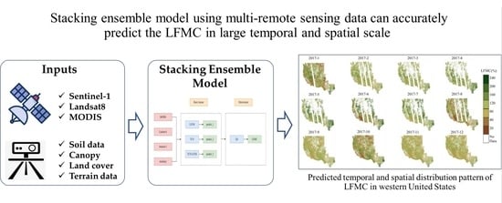
- We explore the advantages of LFMC retrieval utilizing multi-source remote sensing data obtained from combing MODIS, Landsat-8, Sentinel-1 and auxiliary data such as canopy height and land cover as data sources, which can provide more comprehensive data and avoid the limitations of single-source remote sensing data.
- (2)
- We propose a LFMC retrieval model integrating the LSTM and TCN, which exploits the long-time memory capability of LSTM and the superior feature extraction capability of TCN, and finally performs better than LSTM and the TCN alone.
- (3)
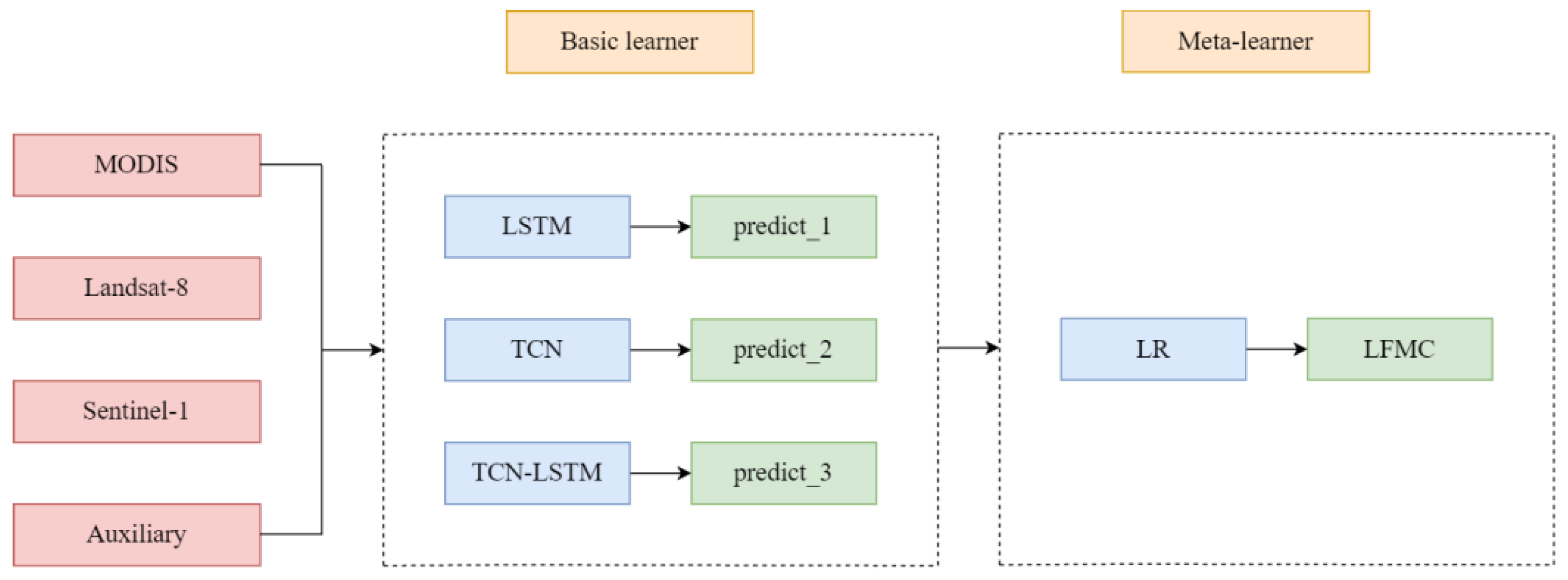
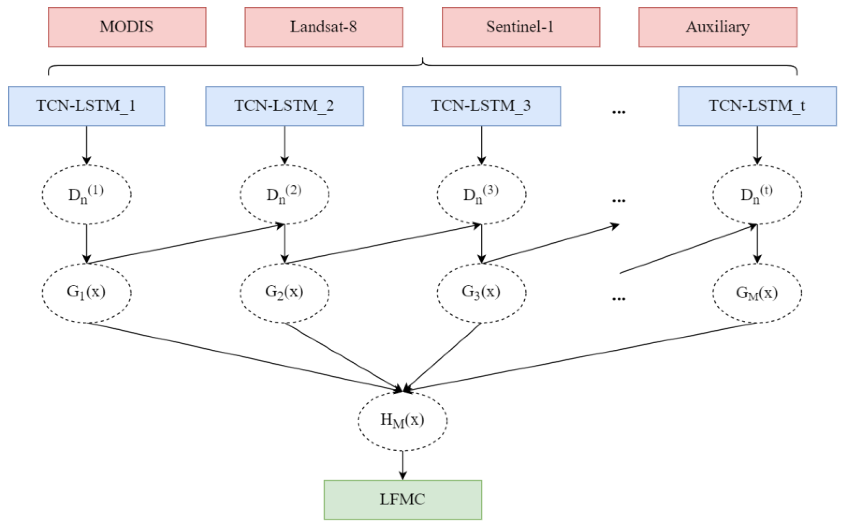
- Based on LSTM, TCN and TCN-LSTM models, two ensemble models (the stacking and Adaboost ensemble models) are designed, and the advantages of stacking ensemble model are confirmed by comparative experiments.
2. Data and Methods
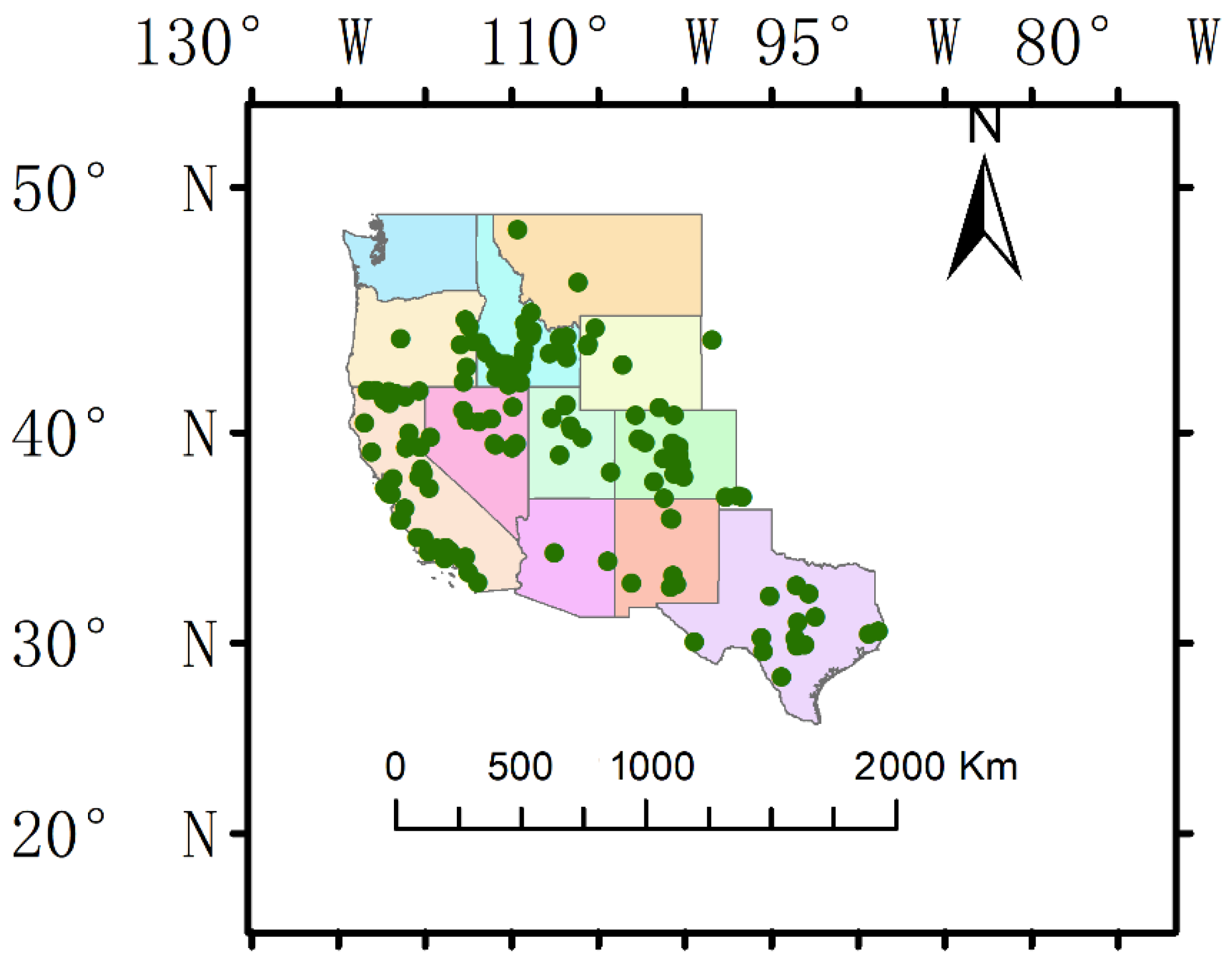
2.1. Study Area
2.2. Research Data
2.2.1. LFMC Data
2.2.2. MODIS Data
2.2.3. Landsat Data
2.2.4. Sentinel-1 Data
2.2.5. Auxiliary Data
2.3. Data Process
2.4. Dataset
2.5. LFMC Retrieval Models
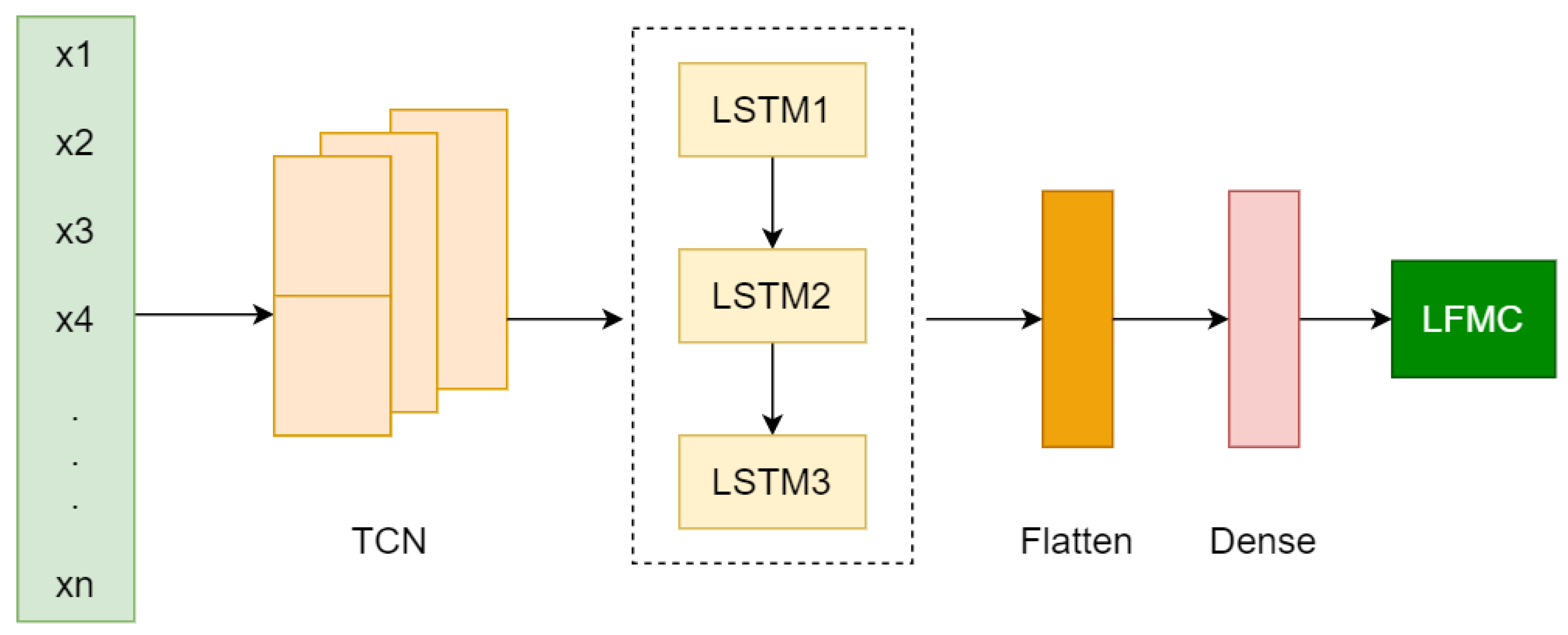
2.5.1. TCN-LSTM Model
- (1)
- Firstly, the LFMC data and selected input variables (x1, …, xn) are fed into the TCN. The features of remote sensing variables and LFMC are extracted through the causal convolution layer contained in the TCN.
- (2)
- Then, multiple LSTM layers combined with the dropout mechanism are used for prediction, which can prevent over fitting.
- (3)
- Through the flatten layer, the output matrix is compressed into one dimension to facilitate the connection of the later dense layer.
- (4)
- The nonlinear relationship is mapped to the output space through the dense layer to achieve the LFMC prediction results.
2.5.2. Stacking Ensemble Model
2.5.3. Adaboost Ensemble Model
2.5.4. Model Settings
3. Experiments and Results
3.1. Experimental Setup
3.2. Evaluating Indicator
3.3. Comparison of Different Deep Learning Models
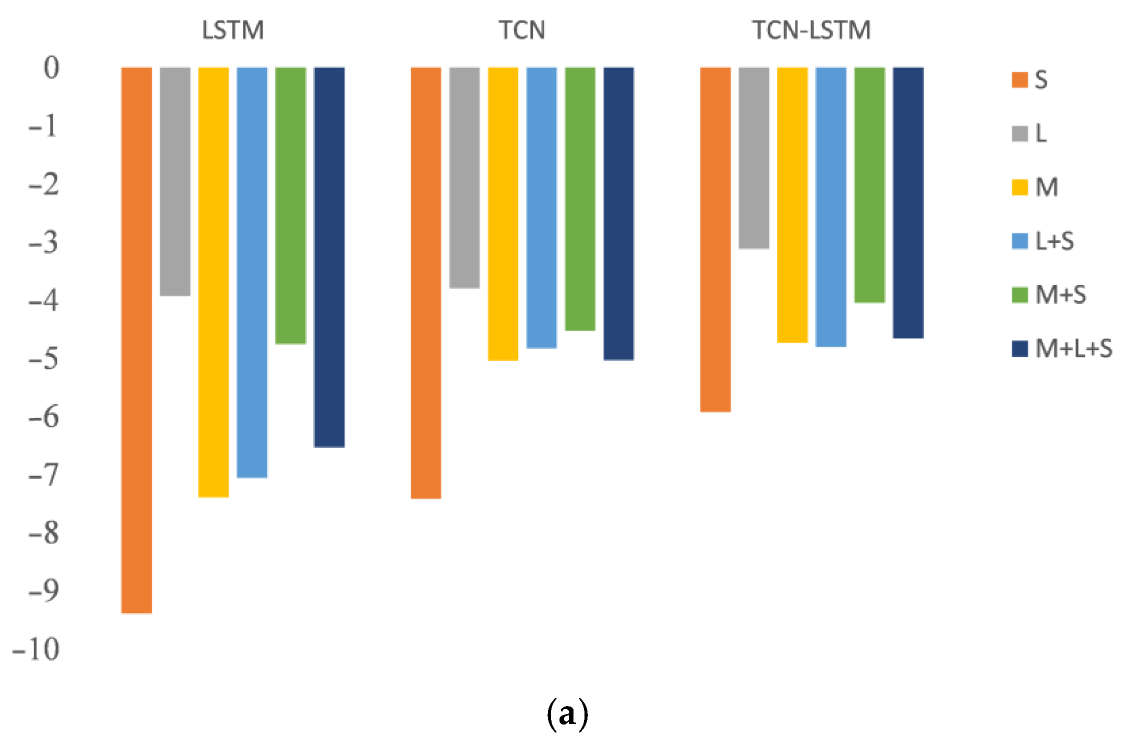
- (1)
- The bias of all the three models was negative, indicating that all the models underestimated LFMC as a whole. The TCN-LSTM model had the lowest bias among all the models on the same dataset. The bias of Sentinel-1 was the largest, and that of Landsat-8 was the lowest. Although microwave remote sensing (Sentinel-1) is more penetrating due to its high sensitivity to surface moisture, it is difficult to distinguish between vegetation and bare soil backscatter only using microwave remote sensing data, which leads to higher bias. The multi-source remote sensing data fuse the microwave remote sensing and optical remote sensing together, which can be essentially seen as the integration of the microwave backscattering characteristics and optical characteristic. Therefore, the retrieval performances of multi-source remote sensing data were higher than those of the single-source remote sensing data.
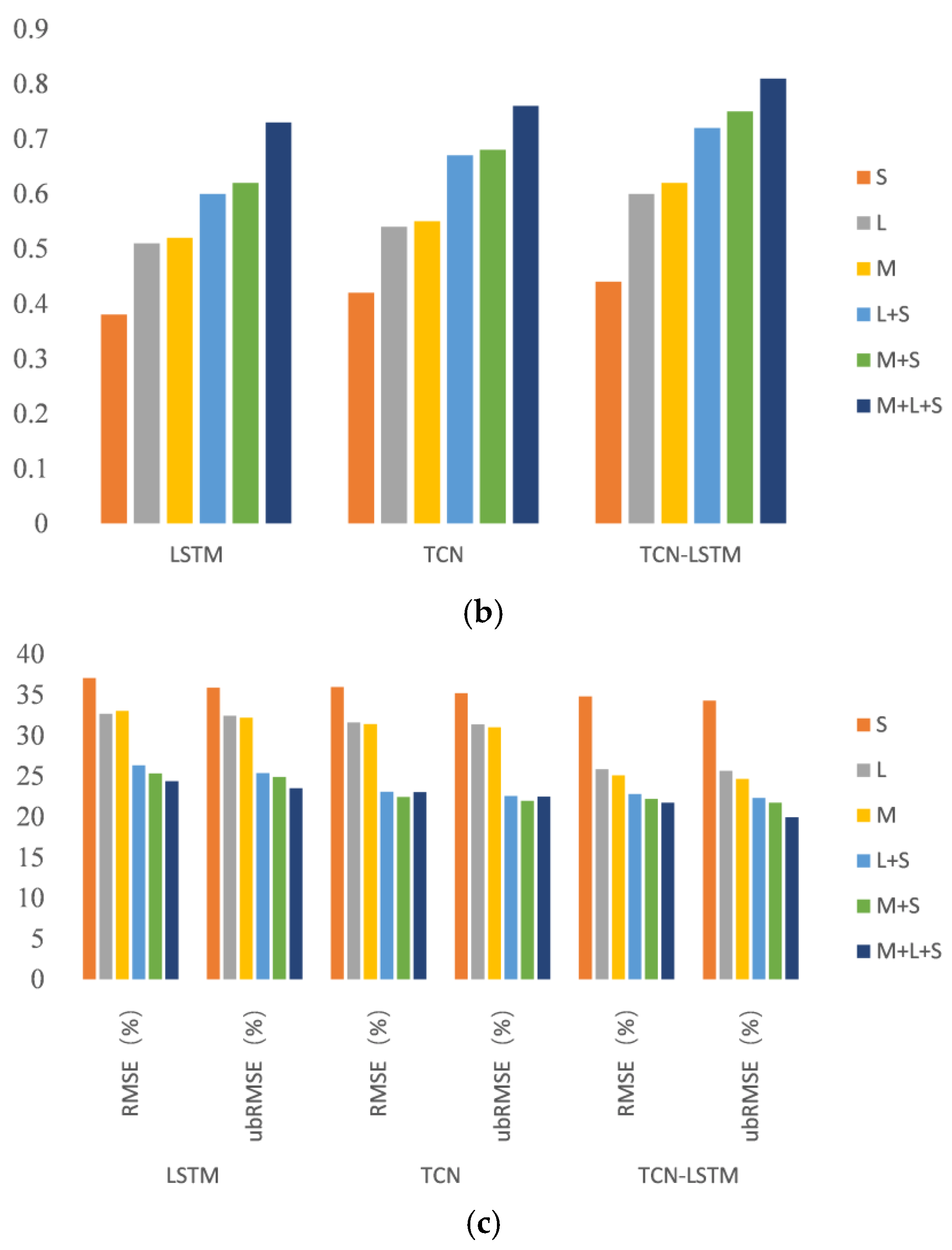
- (2)
- The , RMSE and ubRMSE of the TCN-LSTM model were also better than those of the LSTM and TCN models. The retrieval accuracy of the TCN-LSTM model with all three kinds of remote sensing data was the highest at = 0.81, RMSE = 21.73 and ubRMSE = 19.93, which means that TCN-LSTM can incorporate the advantages of LSTM and the TCN and effectively extract the features of multi-source remote sensing.
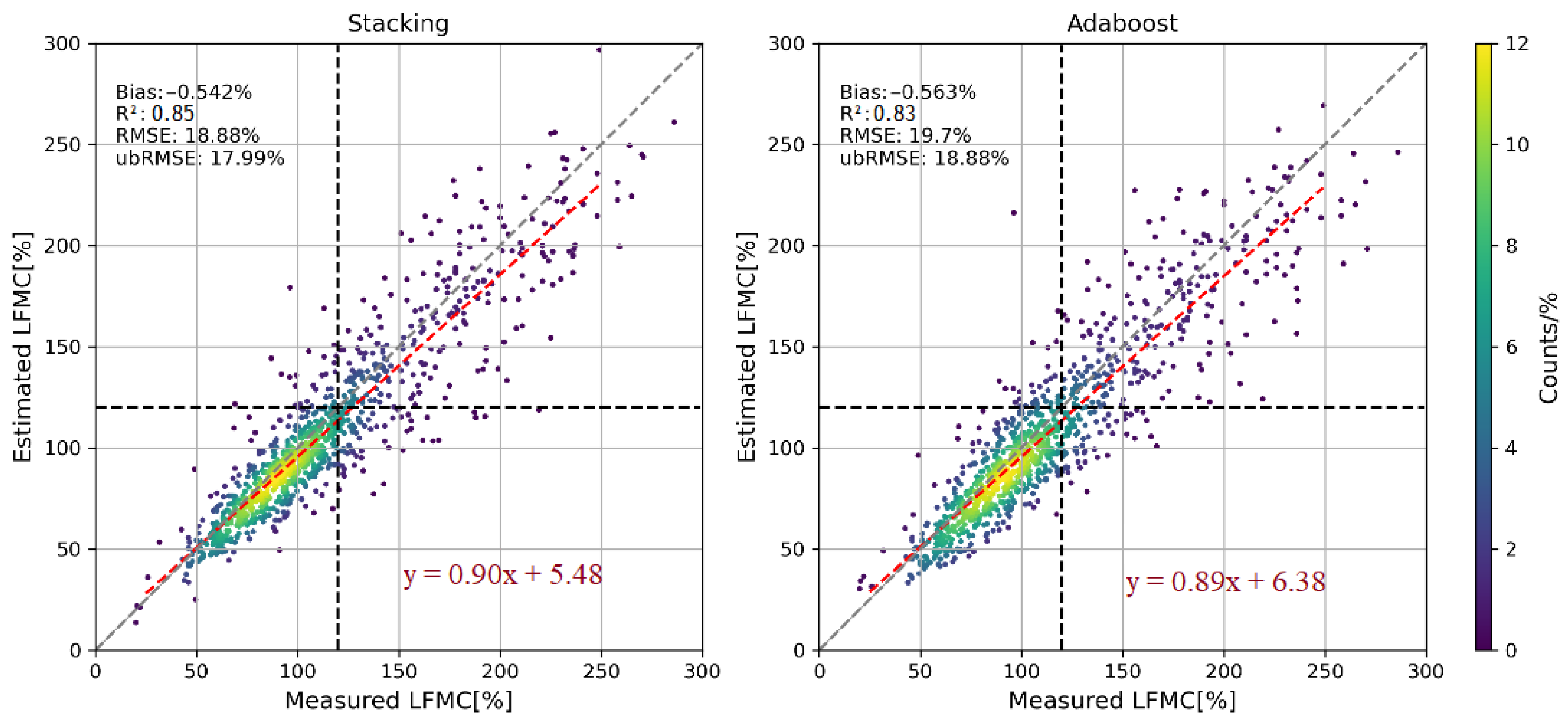
3.4. Comparison of Different Ensemble Learning Models
4. Discussion
4.1. Explanation of Estimated LFMC Value
4.2. Advantages of Multi-Source Remote Sensing Data and Ensemble Learning
4.3. Limitations of the Proposed Method with Processed Data
5. Conclusions
Author Contributions
Funding
Data Availability Statement
Acknowledgments
Conflicts of Interest
References
- Cunill Camprubí, À.; González-Moreno, P.; Resco de Dios, V. Live fuel moisture content mapping in the Mediterranean Basin using random forests and combining MODIS spectral and thermal data. Remote Sens. 2022, 14, 3162. [Google Scholar] [CrossRef]
- Chuvieco, E.; Gonzalez, I.; Verdu, F.; Aguado, I.; Yebra, M. Prediction of fire occurrence from live fuel moisture content measurements in a Mediterranean ecosystem. Int. J. Wildland Fire 2009, 18, 430–441. [Google Scholar] [CrossRef]
- Nolan, R.H.; Boer, M.M.; de Dios, V.R.; Caccamo, G.; Bradstock, R.A. Large-scale, dynamic transformations in fuel moisture drive wildfire activity across southeastern Australia. Geophys. Res. Lett. 2016, 43, 4229–4238. [Google Scholar] [CrossRef]
- Chuvieco, E.; Aguado, I.; Jurdao, S.; Pettinari, M.L.; Yebra, M.; Salas, J.; Hantson, S.; de la Riva, J.; Ibarra, P.; Rodrigues, M.; et al. Integrating geospatial information into fire risk assessment. Int. J. Wildland Fire 2014, 23, 606–619. [Google Scholar] [CrossRef]
- Sibanda, M.; Onisimo, M.; Dube, T.; Mabhaudhi, T. Quantitative assessment of grassland foliar moisture parameters as an inference on rangeland condition in the mesic rangelands of southern Africa. Int. J. Remote Sens. 2021, 42, 1474–1491. [Google Scholar] [CrossRef]
- Yebra, M.; Dennison, P.E.; Chuvieco, E.; Riaño, D.; Zylstra, P.; Hunt, E.R., Jr.; Danson, F.M.; Qi, Y.; Jurdao, S. A global review of remote sensing of live fuel moisture content for fire danger assessment: Moving towards operational products. Remote Sens. Environ. 2013, 136, 455–468. [Google Scholar] [CrossRef]
- Garcia, M.; Chuvieco, E.; Nieto, H.; Aguado, I. Combining AVHRR and meteorological data for estimating live fuel moisture content. Remote Sens. Environ. 2008, 112, 3618–3627. [Google Scholar] [CrossRef]
- García, M.; Riaño, D.; Yebra, M.; Salas, J.; Cardil, A.; Monedero, S.; Ramirez, J.; Martín, M.P.; Vilar, L.; Gajardo, J.; et al. A live fuel moisture content product from Landsat TM satellite time series for implementation in fire behavior models. Remote Sens. 2020, 12, 1714. [Google Scholar] [CrossRef]
- Myoung, B.; Kim, S.H.; Nghiem, S.V.; Jia, S.; Whitney, K.; Kafatos, M.C. Estimating live fuel moisture from MODIS satellite data for wildfire danger assessment in Southern California USA. Remote Sens. 2018, 10, 87. [Google Scholar] [CrossRef]
- Maffei, C.; Menenti, M. A MODIS-based perpendicular moisture index to retrieve leaf moisture content of forest canopies. Int. J. Remote Sens. 2014, 35, 1829–1845. [Google Scholar] [CrossRef]
- Quan, X.; He, B.; Yebra, M.; Yin, C.; Liao, Z.; Li, X. Retrieval of forest fuel moisture content using a coupled radiative transfer model. Environ. Model. Softw. 2017, 95, 290–302. [Google Scholar] [CrossRef]
- Yebra, M.; Van Dijk, A.; Leuning, R.; Huete, A.; Guerschman, J.P. Evaluation of optical remote sensing to estimate actual evapotranspiration and canopy conductance. Remote Sens. Environ. 2013, 129, 250–261. [Google Scholar] [CrossRef]
- Song, C.H. Optical remote sensing of forest leaf area index and biomass. Prog. Phys. Geogr. -Earth Environ. 2013, 37, 98–113. [Google Scholar] [CrossRef]
- Quan, X.; He, B.; Li, X.; Liao, Z. Retrieval of Grassland live fuel moisture content by parameterizing radiative transfer model with interval estimated LAI. IEEE J. Sel. Top. Appl. Earth Obs. Remote Sens. 2016, 9, 910–920. [Google Scholar] [CrossRef]
- Xiao, Z.; Song, J.; Yang, H.; Sun, R.; Li, J. A 250 m resolution global leaf area index product derived from MODIS surface reflectance data. Int. J. Remote Sens. 2022, 43, 1409–1429. [Google Scholar] [CrossRef]
- Al-Moustafa, T.; Armitage, R.P.; Danson, F.M. Mapping fuel moisture content in upland vegetation using airborne hyperspectral imagery. Remote Sens. Environ. 2012, 127, 74–83. [Google Scholar] [CrossRef]
- Houborg, R.; Anderson, M.; Daughtry, C. Utility of an image-based canopy reflectance modeling tool for remote estimation of LAI and leaf chlorophyll content at the field scale. Remote Sens. Environ. 2009, 113, 259–274. [Google Scholar] [CrossRef]
- Fan, L.; Wigneron, J.P.; Xiao, Q.; Al-Yaari, A.; Wen, J.; Martin-StPaul, N.; Dupuy, J.-L.; Pimont, F.; Al Bitar, A.; Fernandez-Moran, R.; et al. Evaluation of microwave remote sensing for monitoring live fuel moisture content in the Mediterranean region. Remote Sens. Environ. 2018, 205, 210–223. [Google Scholar] [CrossRef]
- Rao, K.; Williams, A.P.; Flefil, J.F.; Konings, A.G. SAR-enhanced mapping of live fuel moisture content. Remote Sens. Environ. 2020, 245, 111797. [Google Scholar] [CrossRef]
- Wang, L.; Quan, X.W.; He, B.B.; Yebra, M.; Xing, M.; Liu, X. Assessment of the dual polarimetric Sentinel-1A data for forest fuel moisture content estimation. Remote Sens. 2019, 11, 1568. [Google Scholar] [CrossRef] [Green Version]
- Bai, X.; He, B.; Li, X.; Zeng, J.; Wang, X.; Wang, Z.; Zeng, Y.; Su, Z. First assessment of Sentinel-1A data for surface soil moisture estimations using a coupled water cloud model and advanced integral equation model over the Tibetan Plateau. Remote Sens. 2017, 9, 714. [Google Scholar] [CrossRef]
- Bai, X.; He, B. Potential of Dubois model for soil moisture retrieval in prairie areas using SAR and optical data. Int. J. Remote Sens. 2015, 36, 5737–5753. [Google Scholar] [CrossRef]
- Jiao, W.; Wang, L.; McCabe, M.F. Multi-sensor remote sensing for drought characterization: Current status, opportunities and a roadmap for the future. Remote Sens. Environ. 2021, 256, 112313. [Google Scholar] [CrossRef]
- Reichstein, M.; Camps-Valls, G.; Stevens, B.; Jung, M.; Denzler, J.; Carvalhais, N.; Prabhat. Deep learning and process understanding for data-driven Earth system science. Nature 2019, 566, 195–204. [Google Scholar] [CrossRef]
- Yuan, Q.Q.; Shen, H.F.; Li, T.W.; Li, Z.; Li, S.; Jiang, Y.; Xu, H.; Tan, W.; Yang, Q.; Wang, J.; et al. Deep learning in environmental remote sensing: Achievements and challenges. Remote Sens. Environ. 2020, 241, 111716. [Google Scholar] [CrossRef]
- Zhu, L.; Webb, G.I.; Yebra, M.; Scortechini, G.; Miller, L.; Petitjean, F. Live fuel moisture content estimation from MODIS: A deep learning approach. ISPRS J. Photogramm. Remote Sens. 2021, 179, 81–91. [Google Scholar] [CrossRef]
- United States Forest Sevices. National Fuel Moisture Database; United States Forest Services: Washington, DC, USA, 2010.
- Nietupski, T.C.; Kennedy, R.E.; Temesgen, H.; Kerns, B.K. Spatiotemporal image fusion in Google Earth Engine for annual estimates of land surface phenology in a heterogenous landscape. Int. J. Appl. Earth Obs. Geoinf. 2021, 99, 102323. [Google Scholar] [CrossRef]
- Faiz, M.A.; Liu, D.; Tahir, A.A.; Li, H.; Fu, Q.; Adnan, M.; Zhang, L.; Naz, F. Comprehensive evaluation of 0.25° precipitation datasets combined with MOD10A2 snow cover data in the ice-dominated river basins of Pakistan. Atmos. Res. 2020, 231, 104653. [Google Scholar] [CrossRef]
- Vermote, E.; Justice, C.; Claverie, M.; Franch, B. Preliminary analysis of the performance of the Landsat 8/OLI land surface reflectance product. Remote Sens. Environ. 2016, 185, 46–56. [Google Scholar] [CrossRef]
- Roberts, D.A.; Dennison, P.E.; Peterson, S.; Sweeney, S.; Rechel, J. Evaluation of airborne visible/infrared imaging spectrometer (AVIRIS) and moderate resolution imaging spectrometer (MODIS) measures of live fuel moisture and fuel condition in a shrubland ecosystem in southern California. J. Geophys. Res. -Biogeosci. 2006, 111, 1–16. [Google Scholar] [CrossRef] [Green Version]
- Colombo, R.; Merom, M.; Marchesi, A.; Busetto, L.; Rossini, M.; Giardino, C.; Panigada, C. Estimation of leaf and canopy water content in poplar plantations by means of hyperspectral indices and inverse modeling. Remote Sens. Environ. 2008, 112, 1820–1834. [Google Scholar] [CrossRef]
- Chuvieco, E.; Aguado, I.; Dimitrakopoulos, A.P. Conversion of fuel moisture content values to ignition potential for integrated fire danger assessment. Can. J. For. Res. 2004, 34, 2284–2293. [Google Scholar] [CrossRef]
- Badgley, G.; Field, C.B.; Berry, J.A. Canopy near-infrared reflectance and terrestrial photosynthesis. Sci. Adv. 2017, 3, e1602244. [Google Scholar] [CrossRef]
- Torres, R.; Snoeij, P.; Geudtner, D.; Bibby, D.; Davidson, M.; Attema, E.; Potin, P.; Rommen, B.; Floury, N.; Brown, M.; et al. GMES Sentinel-1 mission. Remote Sens. Environ. 2012, 120, 9–24. [Google Scholar] [CrossRef]
- Keane, R.E. Fuel concepts. In Wildland Fuel Fundamentals and Applications; Springer: Cham, Switzerland, 2015; pp. 175–184. [Google Scholar]
- Brocca, L.; Crow, W.T.; Ciabatta, L.; Massari, C.; de Rosnay, P.; Enenkel, M.; Hahn, S.; Amarnath, G.; Camici, S.; Tarpanelli, A.; et al. A review of the applications of ASCAT soil moisture products. IEEE J. Sel. Top. Appl. Earth Obs. Remote Sens. 2017, 10, 2285–2306. [Google Scholar] [CrossRef]
- Datta, S.; Das, P.; Dutta, D.; Giri, R.K. Estimation of surface moisture content using Sentinel-1 C-band SAR data through machine learning models. J. Indian Soc. Remote Sens. 2020, 49, 887–896. [Google Scholar] [CrossRef]
- Liu, S.; Wei, Y.; Post, W.M.; Cook, R.B.; Schaefer, K.; Thornton, M.M. NACP MsTMIP: Unified North American Soil Map; ORNL Distributed Active Archive Center: Oak Ridge, TN, USA; p. 2014.
- Simard, M.; Pinto, N.; Fisher, J.B.; Baccini, A. Mapping forest canopy height globally with spaceborne lidar. J. Geophys. Res. -Biogeosci. 2011, 116, G04021. [Google Scholar] [CrossRef]
- Arino, O.; Ramos, J.; Kalogirou, V.; Bontemps, S.; Defourny, P.; Van Bogaert, E. Global Land Cover Map for 2009 (GlobCover 2009); European Space Agency (ESA): Paris, France; Université catholique de Louvain (UCL), PANGAEA: Ottignies-Louvain-la-Neuve, Belgium. [CrossRef]
- USGS-NED. National Elevation Dataset; US Geological Survey: Lafayette, LA, USA, 2004.
- Pelletier, C.; Webb, G.I.; Petitjean, F. Temporal convolutional neural network for the classification of satellite image time series. Remote Sens. 2019, 11, 523. [Google Scholar] [CrossRef]
- Jia, S.; Kim, S.H.; Nghiem, S.V.; Kafatos, M. Estimating live fuel moisture using SMAP L-band radiometer soil moisture for Southern California, USA. Remote Sens. 2019, 11, 1575. [Google Scholar] [CrossRef] [Green Version]
- Yebra, M.; Quan, X.; Riano, D.; Larraondo, P.R.; van Dijk, A.I.J.M.; Cary, G.J. A fuel moisture content and flammability monitoring methodology for continental Australia based on optical remote sensing. Remote Sens. Environ. Interdiscip. J. 2018, 212, 260–272. [Google Scholar] [CrossRef]
- Pimont, F.; Ruffault, J.; Martin-StPaul, N.K.; Dupuy, J.-L. Why is the effect of live fuel moisture content on fire rate of spread underestimated in field experiments in shrublands? Int. J. Wildland Fire 2019, 28, 127–137. [Google Scholar] [CrossRef]
- Yebra, M.; Scortechini, G.; Badi, A.; Beget, M.E.; Boer, M.M.; Bradstock, R.; Chuvieco, E.; Danson, F.M.; Dennison, P.; de Dios, V.R.; et al. Globe-LFMC, a global plant water status database for vegetation ecophysiology and wildfire applications. Sci. Data 2019, 6, e155. [Google Scholar] [CrossRef] [PubMed]
- Jurdao, S.; Chuvieco, E.; Arevalillo, J.M. Modelling fire ignition probability from satellite estimates of live fuel moisture content. Fire Ecol. 2012, 8, 77–97. [Google Scholar] [CrossRef]

| MODIS | Landsat-8 | Sentinel-1 | Auxiliary Variables |
|---|---|---|---|
| Band1 | red | Silt content | |
| Band2 | green | Sand content | |
| Band3 | blue | Clay content | |
| Band4 | NIR | Canopy height (m) | |
| Band5 | SWIR | Land cover | |
| Band6 | NDWI | Altitude (m) | |
| Band7 | NDVI | Slope (°) | |
| NIRV |
| LSTM | TCN | TCN-LSTM | |||
|---|---|---|---|---|---|
| Layer | Output Shape | Layer | Output Shape | Layer | Output Shape |
| LSTM | (32,4,10) | Conv1D | (32,365,64) | Conv1D | (32,4,32) |
| LSTM | (32,4,10) | AvgPool | (32,182,64) | Conv1D | (32,4,32) |
| LSTM | (32,10) | Conv1D | (32,182,64) | MaxPool | (32,2,32) |
| Dense | (32,1) | AvgPool | (32,60,64) | Flatten | (32,64) |
| Conv1D | (32,60,64) | RepeatVector | (32,1941,64) | ||
| MaxPool | (32,15,64) | LSTM | (32,1941,10) | ||
| Flatten | (32,960) | LSTM | (32,1941,10) | ||
| Dense | (32,256) | LSTM | (32,10) | ||
| Dense | (32,1) | Dense | (32,1) | ||
| Data | Model | Bias (%) | R2 | RMSE (%) | ubRMSE (%) |
|---|---|---|---|---|---|
| S | LSTM | −9.39 | 0.38 | 37.07 | 35.86 |
| TCN | −7.42 | 0.42 | 35.97 | 35.2 | |
| TCN-LSTM | −5.93 | 0.44 | 34.81 | 34.3 | |
| L | LSTM | −3.93 | 0.51 | 32.67 | 32.43 |
| TCN | −3.8 | 0.54 | 31.58 | 31.35 | |
| TCN-LSTM | −3.12 | 0.60 | 25.83 | 25.64 | |
| M | LSTM | −7.39 | 0.52 | 33.01 | 32.17 |
| TCN | −5.04 | 0.55 | 31.39 | 30.98 | |
| TCN-LSTM | −4.74 | 0.62 | 25.11 | 24.66 | |
| L+S | LSTM | −7.06 | 0.60 | 26.32 | 25.35 |
| TCN | −4.83 | 0.67 | 23.05 | 22.54 | |
| TCN-LSTM | −4.81 | 0.72 | 22.78 | 22.31 | |
| M+S | LSTM | −4.76 | 0.62 | 25.33 | 24.88 |
| TCN | −4.53 | 0.68 | 22.43 | 21.97 | |
| TCN-LSTM | −4.05 | 0.75 | 22.21 | 21.71 | |
| M+L+S | LSTM | −6.53 | 0.73 | 24.39 | 23.5 |
| TCN | −5.03 | 0.76 | 23.03 | 22.48 | |
| TCN-LSTM | −4.66 | 0.81 | 21.73 | 19.93 |
| Method | RMSE (%) | |
|---|---|---|
| LSTM (Landsat+SAR) [19] | 0.63 | 25 |
| TempCNN-LFMC (MODIS+Auxiliary data) [20] | 0.64 | 22.74 |
| TCN-LSTM model | 0.81 | 21.73 |
| Data | Stacking | Adaboost | ||||||
|---|---|---|---|---|---|---|---|---|
| Bias (%) | RMSE (%) | ubRMSE (%) | Bias (%) | RMSE (%) | ubRMSE (%) | |||
| S | −5.75 | 0.53 | 31.87 | 31.35 | −4.59 | 0.53 | 31.62 | 31.29 |
| L | −3.35 | 0.7 | 23.26 | 23.21 | −1.65 | 0.65 | 23.6 | 23.54 |
| M | −4.55 | 0.74 | 23.82 | 23.39 | −4.16 | 0.68 | 22.53 | 22.14 |
| L+S | −1.55 | 0.81 | 19.96 | 19.95 | −2.61 | 0.76 | 22 | 21.31 |
| M+S | −1.43 | 0.81 | 19.86 | 19.81 | −2.7 | 0.8 | 20.5 | 20.32 |
| M+L+S | −0.542 | 0.85 | 18.88 | 17.99 | −0.563 | 0.83 | 19.7 | 18.8 |
Publisher’s Note: MDPI stays neutral with regard to jurisdictional claims in published maps and institutional affiliations. |
© 2022 by the authors. Licensee MDPI, Basel, Switzerland. This article is an open access article distributed under the terms and conditions of the Creative Commons Attribution (CC BY) license (https://creativecommons.org/licenses/by/4.0/).
Share and Cite
Xie, J.; Qi, T.; Hu, W.; Huang, H.; Chen, B.; Zhang, J. Retrieval of Live Fuel Moisture Content Based on Multi-Source Remote Sensing Data and Ensemble Deep Learning Model. Remote Sens. 2022, 14, 4378. https://doi.org/10.3390/rs14174378
Xie J, Qi T, Hu W, Huang H, Chen B, Zhang J. Retrieval of Live Fuel Moisture Content Based on Multi-Source Remote Sensing Data and Ensemble Deep Learning Model. Remote Sensing. 2022; 14(17):4378. https://doi.org/10.3390/rs14174378
Chicago/Turabian StyleXie, Jiangjian, Tao Qi, Wanjun Hu, Huaguo Huang, Beibei Chen, and Junguo Zhang. 2022. "Retrieval of Live Fuel Moisture Content Based on Multi-Source Remote Sensing Data and Ensemble Deep Learning Model" Remote Sensing 14, no. 17: 4378. https://doi.org/10.3390/rs14174378
APA StyleXie, J., Qi, T., Hu, W., Huang, H., Chen, B., & Zhang, J. (2022). Retrieval of Live Fuel Moisture Content Based on Multi-Source Remote Sensing Data and Ensemble Deep Learning Model. Remote Sensing, 14(17), 4378. https://doi.org/10.3390/rs14174378