Joint Flying Relay Location and Routing Optimization for 6G UAV–IoT Networks: A Graph Neural Network-Based Approach

Abstract

Unmanned aerial vehicles (UAVs) are widely used in Internet-of-Things (IoT) networks, especially in remote areas where communication infrastructure is unavailable, due to flexibility and low cost. However, the joint optimization of locations of UAVs and relay path selection can be very challenging, especially when the numbers of IoT devices and UAVs are very large. In this paper, we formulate the joint optimization of UAV locations and relay paths in UAV-relayed IoT networks as a graph problem, and propose a graph neural network (GNN)-based approach to solve it in an efficient and scalable way. In the training procedure, we design a reinforcement learning-based relay GNN (RGNN) to select the best relay path for each user. The theoretical analysis shows that the time complexity of RGNN is two orders lower than the conventional optimization method. Then, we jointly exploit location GNN (LGNN) and RGNN trained to optimize the locations of all UAVs. Both GNNs can be trained without relying on the training data, which is usually unavailable in the context of wireless networks. In inference procedure, LGNN is first used to optimize the location of UAVs, and then RGNN is used to select the best relay path based on the output of LGNN. Simulation results show that the proposed approach can achieve comparable performance to brute-force search with much lower time complexity when the network is relatively small. Remarkably, the proposed approach is highly scalable to large-scale networks and adaptable to dynamics in the environment, which can hardly be achieved using conventional methods.

1. Introduction

With the trend of seamless connection and supporting vertical services, in 6G networks, there will be a large amount of Internet-of-Things (IoT) devices deployed in diverse scenarios to carry a wide range of applications, such as data collection and emergency detection [1,2,3]. However, most IoT devices may be deployed in remote areas such as remote suburban and rural areas, even mountains and deserts. In such regions, IoT devices cannot communicate with others directly due to the long distance between them, and infrastructures like base stations (BSs) are usually missing due to high economic costs [4,5,6]. Therefore, it is necessary to deploy flexible and low-cost relays to satisfy the communication demands of IoT devices [7]. As a promising technology, unmanned aerial vehicles (UAVs) have attracted much attention from wireless communications researchers due to their flexibility and low cost. According to [8], the research on UAVs in wireless communications can be divided into three main directions, UAV-aided ubiquitous coverage, information dissemination, and relaying. It has been demonstrated that a UAV can be used to extend the coverage of wireless networks, provide services to more users [4], and enhance communication performance for remote users in wireless networks [6,9,10,11].

Nowadays, many methods have been used to optimize the performance of UAV networks, e.g., convex optimization [5], stochastic geometry [12], and learning-based strategy [4,13]. However, in sixth generation (6G) communication networks, especially in IoT networks, there are five main challenges to the application of traditional optimization technology or learning-based methods.

• High performance. In a 6G network, there will be a large amount of image and video monitoring tasks for IoT devices, and transmitting such data requires high communication rates [1]. It is usually required to jointly optimize the trajectories, relay paths, transmit powers, and so forth of the UAVs and IoT devices to maximize the communication rates. However, this joint optimization is generally not a convex problem, and it is challenging to find the optimal solution quickly [5]. In addition, traditional optimization methods such as alternating minimization (AM) algorithm usually fall into the false local optimal [14].
• High efficiency. In the 6G IoT network, the number of IoT devices can be very large, and thus the algorithm’s time complexity should be very low to deal with the large-scale optimization problem [15]. In addition, the ultra-low latency requirements of certain 6G services make the algorithm’s execution time significantly affect the quality of service (QoS), examples of which are mobile IoT services [16]. Therefore, the algorithm should be executed by the system in a very efficient way such that the QoS can be improved. Thus, exploiting traditional optimization and heuristic algorithms is challenging since they usually need a long time to generate a solution, especially when the network scale is large.
• High Robustness. As IoT devices may be moving, the algorithm should be robust to small changes in the locations of the IoT device, i.e., the optimization results can be directly inferred from the algorithm without iteration-based execution or re-training. Traditional optimization algorithms need to be executed again as long as the environment changes, resulting in extra delays when the environment is not sTable Unfortunately, using traditional neural network (NN) methods is challenging due to their low generalizability [17].
• High Scalability. In 6G networks, there will be many periodic hibernations and time-triggered switch-on IoT devices [18]. Thus, the scale of the network can be changed at different times. This requires the algorithm to be scalable to the increasing/decreasing number of users in the network. However, traditional multi-layer perception (MLP), convolutional neural networks (CNN), and recurrent neural networks (RNN), even attention-based transformer network has no such scalability [19].
• Low complexity. Usually, in UAV networks the optimization algorithm runs on the UAV’s processor. However, it is difficult for UAVs to carry high-performance computing chips due to limitations such as UAVs’ weight and energy consumption. Moreover, in 6G IoT networks, the number of users and UAVs might be very large, leading to a possible increase in the algorithm complexity [5]. Therefore, the algorithm should have low time complexity to improve the efficiency and low space complexity such that the algorithm can run on the UAV without memory overflow, even when it deals with very large IoT networks.

In recent years, an emerging neural network architecture named the graph neural network (GNN) has gained increasing attention [20]. GNNs can discover not only features of data but also relationships between them using a graph structure, which significantly improves the power to analyze data [21]. Therefore, GNN has been successfully applied in many fields, e.g., community detection [22], drug design [23], and combinatorial optimization [24]. Furthermore, the message passing mechanism in GNN is highly consistent with distributed optimization algorithms [25]. Thus, GNN-based optimization algorithms are successful in several areas of wireless communication networks, such as power allocation [19], signal detection [26], network slicing [27], and virtual network function (VNF) design [28]. Due to the message passing mechanism, GNNs do not need to process data from all users simultaneously but only from each user locally. Therefore, the number of trainable parameters in GNNs is significantly lower than in traditional neural network architectures such as MLPs and CNNs, inducing much lower computational complexity [29]. This allows GNNs to be easily deployed in UAVs with poor computational and storage capabilities. Moreover, as the message passing of GNN is structure-independent, the GNN has good scalability and can flexibly cope with network scenarios with different numbers of users and topologies.

In this paper, we focus on a general scenario in remote areas with no terrestrial communication infrastructures, where multiple IoT devices communicate with others using UAVs as relays. Inspired by the above distinctive features of GNN, we proposed a GNN-based method to jointly optimize UAV-relay location and routing in order to enable efficient simultaneous data transmissions among multiple pairs of ground IoT devices. The major contributions are summarized as follows.

(1)

We model the problem of joint relay path selection and UAV location optimization in multi-user multi-UAV networks as a graph optimization problem and solve it using a GNN-based approach. Compared with traditional optimization-based methods and non-GNN neural network-based methods, GNN models have the benefits of flexible structure, lower computation requirement, and fast convergence, making them very suitable in dynamic environments of UAV networks and UAVs with low power and computation capabilities.

(2)

We propose a two-stage GNN-based optimization framework. The problem is decoupled into optimal relay path selection and UAV position optimization, each of which is solved by an individual GNN model. Through this, the complexity of the initial problem is significantly reduced, and the learning convergence and performance are improved.

(3)

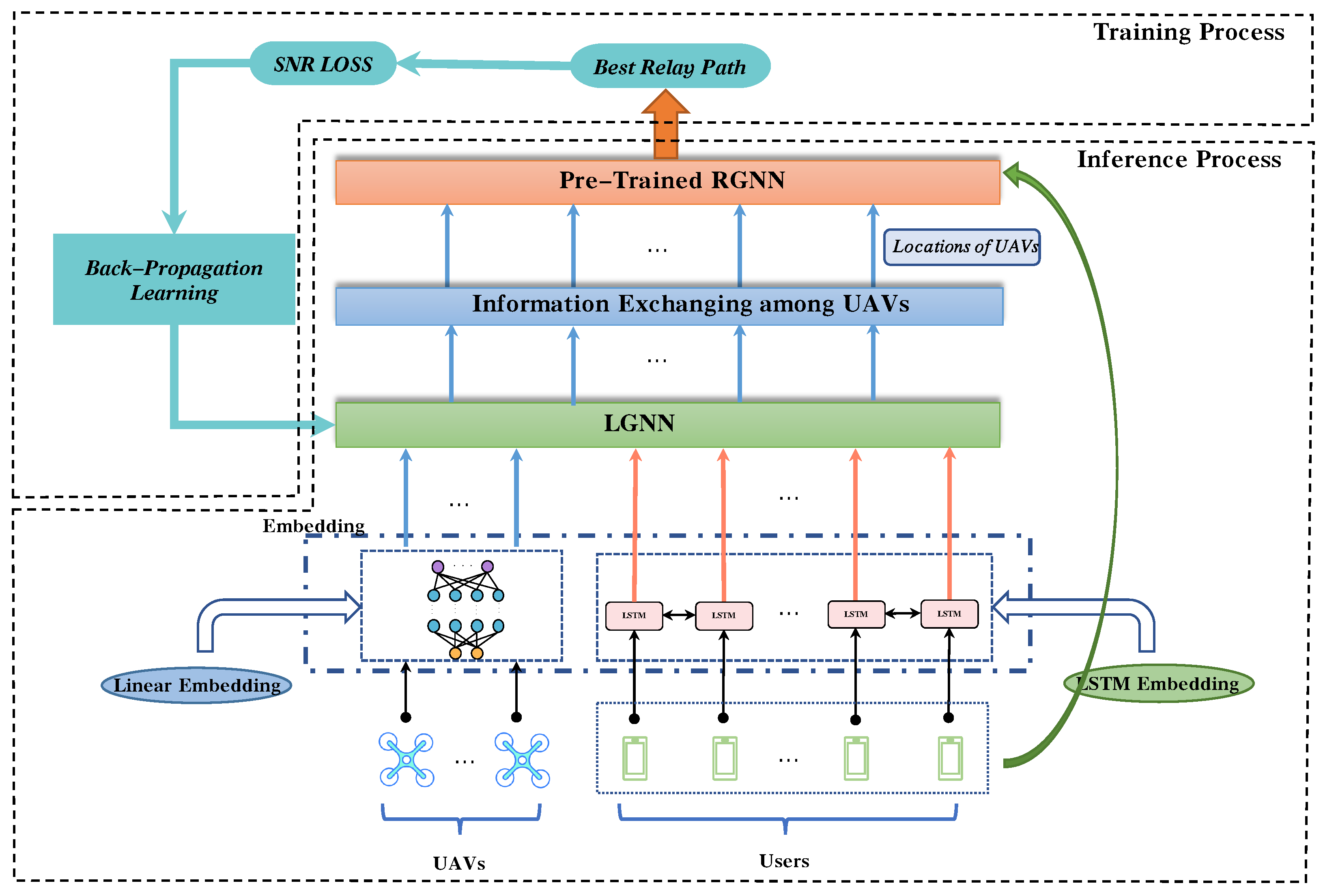
With the two-stage framework, in the training procedure, a relay GNN (RGNN) is first trained to select the best relay path, and a location GNN (LGNN) is trained to optimize the locations of UAV relays with trained RGNN to select the paths such that the loss of LGNN can be calculated. Specifically, we exploit reinforcement learning and unsupervised learning to train RGNN and LGNN, respectively, which do not require any training data or knowledge of optimal solutions. In the inference procedure, LGNN is first used to optimize the location of UAVs, and then RGNN is used to select the best relay path based on the location of UAVs optimized by LGNN.

(4)

We evaluate the performance of the proposed method through extensive simulations. The results show that the proposed method achieves comparable performance to brute-force search with much lower time complexity. Furthermore, the proposed method is also scalable to very large networks and can adapt to environmental dynamics, which is significant in UAV–IoT networks.

The remainder of the paper is organized as follows. In Section 2, we give a brief introduction to graph neural networks and long short-term memory. Section 3 describes the system model, and the joint optimization problem of the location of UAVs and relay path selection is formulated. The proposed GNN-based method is described in Section 4. Section 5 evaluates the performance of the proposed method, and Section 6 concludes the paper.

2. Related Work and Preliminary

2.1. Related Work

In recent years, many works focuse on the optimization of the communication quality in IoT networks. Some early studies optimize the location of a single or small number of UAVs [30,31]. The joint location optimization of multi-UAVs has a broader prospect in practical applications. Taking into account the timeliness, Galkin [32] uses the more traditional and efficient Kmeans clustering algorithm to plan the location of each UAV and determine the service objects of each UAV with high efficiency but sacrificing some performance. With higher optimization requirements, most studies are proposed based on convex optimization and evolution algorithms.

In the deployment of multiple UAVs, some works obtain local optimal solutions based on the local information. For example, in the research of Huang [33], the coverage maximization algorithm is used to find the local optimal solution, which only needs local information. The calculation of the algorithm is simple and can be completed in real-time. Another work from Huang [34] uses a distributed solution. An efficient sub-region partitioning method is proposed to make each UAV serve almost equal traffic demands and minimize the maximum traffic demand of the sub-regions under the constraints of the traffic demand and the shape of the sub-regions. Besides, a local search procedure to relocate the UAV using the backtracking line search algorithm is proposed in this work. Solutions based on local information are usually easier to achieve fast solutions, but usually, only locally optimal solutions can be obtained, which can be useful in some specific situations. There is more work using global information to optimize UAV locations.

Since there are many works focusing on linear programming and other convex optimization methods to solve the UAV deployment problem, the work of Cicek [35] conducts a comprehensive survey of the literature on UAV position optimization. In this work, a general optimization framework is constructed through a general mixed integer nonlinear programming (MINLP) formulation, and the specification of its components is specified. Sabzehali [36] formulates the UAV locations optimization problem as integer linear programming and proposed a low-complexity algorithm. A novelty work from Kang [37] proposes placement learning based on Gibbs-sampling-based (GSB), which gradually learns sub-optimal UAV locations by generating a series of sampling for the UAV locations that constitute a Markov chain where the transition probability determined by the maximum and minimum rates of the different configurations placed by the UAV. However, this work is difficult to adapt to dynamic IoT networks, and the convergence speed is highly dependent on the initial UAV locations. The methods based on linear programming and convex optimization usually achieve satisfactory solutions, but the time complexity is high, and they are usually difficult to adapt to dynamic IoT networks. Especially for large-scale IoT networks, it is difficult to obtain a better solution in real-time.

Since UAV location optimization problems are often modelled as non-convex problems such as mixed-integer optimization problems, which is difficult for convex optimization to obtain a better solution in real-time, heuristic algorithms, especially genetic algorithms, are also often used to optimize UAV deployment problems. Košmerl [38] proposed a method with the genetic algorithm as the core principle for complete coverage with a minimum number of UAVs for Portable Ground Station and Low Altitude Platform. Kalantari [39] proposed a heuristic algorithm based on particle swarm optimization. In this work, the number of UAVs and their 3D layouts are estimated while the coverage and capacity constraints of the system are satisfied. Otherwise, Plachy [40] investigated the performance of two joint association and localization methods based on Genetic Algorithm (GA) and Particle Swarm Optimization (PSO). The methods based on the evolution algorithm can usually achieve satisfactory results, but it is difficult to obtain a solution in a short time, especially with rapidly changing IoT communication requirements.

With the rapid development of deep learning, more and more scholars use deep learning technology to solve UAV-Assisted communication-related problems [41]. In [42] a CNN-based method is used to optimize the placement of the sensor in the sensors network, and in [43] DDQN is used to solve the task scheduling problem by RL. The actor-critic-based RL method is proposed to solve the comprehensive offloading problem in satellite-UAV-ground network [4]. However, there are relatively few related studies optimizing the location of UAVs through the deep neural network model directly. Our paper contributes a scheme of using neural networks to optimize UAV locations.

2.2. Preliminary

2.2.1. Graph Neural Networks

GNN is designed to deal with the problems associated with a graph which is of non-euclidean structure. A graph consists of a node-set and an edge set. Each node v has feature $x_v$, and node v is connected with its neighbouring nodes through edges. GNN propagates and aggregates features through edges to learn the representation of nodes. The main purpose of GNN is to study node features $x_v$ by extracting information from neighbouring nodes [44]. The most important part of the GNN structure is the message passing mechanism, including message propagation and message aggregation. The framework of GNN is described as

$$\begin{array}{cc}\hfill & m_u^v=\varphi (x_v^{l-1},x_u^{l-1})\forall u\in \mathcal{N}\left(v\right),\hfill \end{array}$$

(1)

$$\begin{array}{cc}\hfill & x_v^l=\Psi (x_v^{l-1},\rho \left(\{m_u^v:u\in \mathcal{N}\left(v\right)\}\right)).\hfill \end{array}$$

(2)

where $\mathcal{N}\left(v\right)$ is the set of neighboring nodes of node v. $x_v^{l-1}$ is the feature of node v in layer $l-1$ and $x_u^{l-1}$ represents the feature of one neighboring node u. $\varphi (·)$ represents the parametric message propagation function which determines the message passing from neighbourhood u to node v. $m_u^v$ represents the message propagated from neighboring node u to v. In Equation (2), $\rho (·)$ represents the aggregation function which aggregates all the message from neighboring nodes. The aggregation function used to be set to “Mean”, “Add” or “Max”. Function $\Psi (·)$ updates the features of node v according to feature $x_v^{l-1}$ and the message aggregated.

2.2.2. Long Short Term Memory

Long short-term memory (LSTM) is a special kind of recurrent neural network (RNN) suitable for learning long sequences. An LSTM block generally consists of a cell state, a hidden state, and three gates, i.e., forget gate, input gate, and output gate. The cell state $c_t$ serves as the memory for storing past inputs’ information. The hidden state $h_t$ is the output vector in the t-th LSTM unit and will be passed to the next LSTM unit. The forget gate $f_t$ determines how much information of cell state $c_{t-1}$ from the last unit will be passed to the current cell state $c_t$. The input gate decides the amount of information of input vector $x_t$ and hidden state $h_{t-1}$ from the last unit delivered to the current cell state $c_t$. Moreover, the output gate determines the information current cell state $c_t$ transferred to the current hidden state $h_t$, which is also used as the output vector. The forget gate, input gate and output gate are given respectively by [45].

$$\begin{array}{cc}\hfill & f_t=\sigma (W_f{x}_t+U_f{h}_{t-1}+b_f),\hfill \end{array}$$

(3)

$$\begin{array}{cc}\hfill & i_t=\sigma (W_i{x}_t+U_i{h}_{t-1}+b_i),\hfill \end{array}$$

(4)

$$\begin{array}{cc}\hfill & o_t=\sigma (W_o{x}_t+U_o{h}_{t-1}+b_o).\hfill \end{array}$$

(5)

where $W_f,W_i$, and $W_o$ are associated with input vector $x_t$ are the weights of forgetting gate, input gate, and output gate, respectively, while the weights $U_f,U_i$, and $U_o$ are associated with hidden state vector $h_{t-1}$. $b_f$, $b_i$, and $b_o$ are the bias vectors. $\sigma (·)$ is the sigmoid function that serves as the activation function. The cell state $c_t$ and hidden state $h_t$ with these gates are updated as

$$\begin{array}{cc}\hfill & c_t=f_t{c}_{t-1}+i_{t}tanh(W_c{x}_t+U_c{h}_{t-1}+b_c),\hfill \end{array}$$

(6)

$$\begin{array}{cc}\hfill & h_t=o_{t}tanh\left(c_t\right),\hfill \end{array}$$

(7)

where $W_c$ and $U_c$ are the weights, and $b_c$ is the bias. LSTM is widely used in processing long sequences, but the order of the information passing affects the representations seriously. BiLSTM [46], with information passing bidirectionally in each layer of LSTM networks, can relieve the impact of the order of information passing.

3. System Model and Problem Formulation

3.1. System Model

In this paper, we consider the scenario that there are multiple IoT devices in remote areas and need to transfer data to other IoT devices, which is very common in intelligent agriculture. The system controller or automatic machinery needs to analyze information from remote areas to determine if specific equipment, i.e. automatic welding machine, automatic pesticide spreader, automatic watering machine, needs to be activated [47,48,49,50]. However, due to the sparse geographical distribution of IoT devices and the lack of terrestrial communication infrastructure in remote areas, IoT devices are considered incapable of communicating with each other directly. Although satellites can be used to support the communication requirement between users, the cost of using satellites is too high, and the moving speed of satellites is too high to provide stable and continuous service to users in a certain area [51]. As a result, in this paper, the satellite is only used as a centralized controller to optimize the location of UAVs and relay paths, while the UAVs are used as mobile relays to assist the data transfer. In this paper, we consider K pairs of IoT senders and receivers (In this paper, we use the term user to represent an IoT device, i.e., a sender and a receiver.) and M UAVs. To simplify the problem, we consider that one IoT sender has the request to transfer data to a specific IoT receiver and vice versa. We further assume that for each UAV, it can communicate with the IoT devices and other UAVs at a distance of up to $\xi$ meters.

To generalize the relay problem, every UAV can be used as the relay node for users and UAVs within the coverage area, and the number of hops is not limited until the user receives the data, thus the minimum number of hops is 1, and the maximum number of hops is the same as the number of UAVs M. In addition, each pair of users selects the relay path respectively, and the number of hops among different pairs of users can be different. For example, in Figure 1 the sender 1 can select UAV 1 or UAV 2 as the first relay hop, as they are within the communication coverage. Then, if UAV 2 receives the data from sender 1, it can transmit the data to receiver 1 or to UAV 3 based on the quality of the link, but UAV 2 cannot transmit data to UAV 1 because this will lead to a loop in relay path. Therefore, there are a total 4 optional relay paths for sender 1, and the relay path selection method of sender 2 is same as sender 1.

Considering the high deploying costs of UAVs, its more efficient to deploy the minimal number of UAVs as long as all IoT users are covered. Thus, similar to [4,5,6] in this paper we focus on the scenario that the $K\gg M$. Obviously, when there are M UAVs in the network, which can cover a maximum network area of $M{\xi }^2\pi$. Therefore, in this paper, the network area is proportional to the maximum coverage area for M UAVs.

To elucidate the essence of the underlying problem and emphasis the influence of location of UAVs and relay path network on average communication rate, in this paper, the simple yet typical orthogonal frequency division multiplexing (OFDM) is considered. Every data link, including UAV–IoT device links and UAV–UAV links, can use a specific frequency with equal bandwidth B to transmit the data. In addition, for simplicity, the transmit powers of all users, including IoT devices and UAVs, are considered the same, denoted by P. Consider a path from a sender device to a receiver device composed of multiple hops, and apparently, the flow rate of the path is determined by the least rate among the hops. Generally, the channel model consists of the large-scale path-loss and the small-scale channel fading, however, since the small-scale channel information changes in the time-scale of millimeter second, it is impossible to design the location of UAVs according to this fast-varying channel state information. Thus, in this paper, only large-scale characteristics are considered [52,53]. Therefore, the flow rate $f_s$ of sender s can be calculated by

$$\begin{array}{cc}\hfill & f_s=\underset{i_s}{min}{r}_{i_s}=\underset{i_s}{min}B{log}_2\left(1+\frac{g_{0}P}{B{N}_0{d}_{i_s}^{\gamma }}\right),\hfill \end{array}$$

(8)

where $r_{i_s}$ is the rate of hop i for data from sender s, $d_{i_s}$ is the distance between the two nodes of hop $i_s$, $g_0$ is the path loss for unit distance, $\gamma$ is the path-loss exponent, and $N_0$ is the additive white Gaussian noise (AWGN) at the receiver. It can been seen from Equation (8) that the flow rate f is finally determined by the hop with minimal distance $d_i$. In this paper, given K pairs of senders and receivers, the UAVs locations and the paths of each pair should be jointly optimized to maximize the total system flow rate, i.e.,

$$\begin{array}{cc}\hfill & max\sum _{j=1}^K{f}_j,\hfill \end{array}$$

(9)

3.2. Problem Formulation

To formulate the problem, we use a weighted undirected graph $\mathcal{G}=(\mathcal{V},\mathcal{E})$ to represent the topology of all users and UAVs. The vertex set $\mathcal{V}$ represents the nodes in the network, including IoT devices and UAVs. The edge set $\mathcal{E}$ represents wireless links. $\mathcal{N}\left(u\right)$ is the set of all neighbour nodes of node-u. The set $\mathcal{V}$ consists sender device set ${\mathcal{V}}_s$, receiver device set ${\mathcal{V}}_r$, and UAV set ${\mathcal{V}}_u$, where $|{\mathcal{V}}_s|=|{\mathcal{V}}_r|=K,|{\mathcal{V}}_u|=M$, thus $\mathcal{V}=\left\{{\mathcal{V}}_s,{\mathcal{V}}_r,{\mathcal{V}}_u\right\}$. Define ${\mathcal{V}}_s^r$ as the set of receivers for sender user s. The feature of node i is its location ${\mathbf{d}}_i$. The link $e_{ij}\in \mathcal{E}$ if and only if $i,j\in {\mathcal{V}}_u$ or $i\in {\mathcal{V}}_s\bigcup {\mathcal{V}}_r,j\in {\mathcal{V}}_u$. The weight of link $e_{ij}$ is the transmission rate $r_{ij}$ between node i and node j.

Given the graph $\mathcal{G}$, we formulate the problem considering the following decision variables:

-

A set of binary variables $\mathcal{X}=\left\{{\mathbf{x}}_1,{\mathbf{x}}_2,\cdots ,{\mathbf{x}}_{|{\mathcal{V}}_s|}\right\}$, where ${\mathbf{x}}_s=\left\{x_s^{ij}|i,j\in \mathcal{V}\right\}$ is set of relay path for sender s, and $x_s^{ij}=1$ if node $i,j$ are used to transmit data from sender i, otherwise $x_s^{ij}=0$.

-

A set of continuous variables $\mathcal{F}=\left\{{\mathbf{f}}_1,{\mathbf{f}}_2,\cdots ,{\mathbf{f}}_{|{\mathcal{V}}_s|}\right\}$, where ${\mathbf{f}}_s=\left\{f_s^{ij}|i,j\in \mathcal{V}\right\}$ is the data flow from sender s, and $f_s^{ij}$ is the amount of traffic from node i to node j to relay data from sender s.

-

A set of continuous variables $\mathcal{D}=\left\{{\mathbf{d}}_1,{\mathbf{d}}_2,\cdots ,{\mathbf{d}}_{|{\mathcal{V}}_u|}\right\}$, where ${\mathbf{d}}_u$ is the location of UAVs u.

Therefore, the problem of maximizing the communication rate for all pairs of users can be formulated as the following network flow maximization problem.

The objective function (17) aims at maximizing the flow from all senders, which is equal to maximizing the sum rate of all pairs of users as Equation (9). Note that when the UAVs position $\mathcal{D}$ and the relay path $\mathcal{X}$ are determined, the value of each f that maximizes the objective function is necessarily equal to the lowest hop rate in the relay path. Therefore, we just need to optimize the UAVs position $\mathcal{D}$, and relay path $\mathcal{X}$. Constraint (11) shows that the flow between two nodes cannot be larger than the communication rate between them. Since the UAVs should transmit all received data to another neighbor nodes, the received flow from all neighbor ${\sum }_{i\in \mathcal{N}\left(j\right)}{x}_s^{ij}{f}_s^{ij}$ should equal to the flow transmitting to other neighbor nodes ${\sum }_{i\in \mathcal{N}\left(j\right)}{x}_s^{ji}{f}_s^{ji}=0$. Constraint (13) ensures the sender’s flow is equal to the receiving flow of its corresponding receiver. Constraints (14) and (15) ensure that the data from sender s is only transmitted to one neighboring node. Constraint (16) determines the communication rate between node i and node j, and when the distance between user and UAV or two UAVs is longer than $\xi$ the communication link between them cannot be established, thus the rate is set to be 0. As mentioned above, to simplify the problem, we assume that $\alpha$ is the same for all nodes, i.e., same transmit power. However, the proposed approach can be easily extended to general cases.

Problem 1. 

$$\begin{array}{cc}\hfill & \underset{\mathcal{X},\mathcal{D}}{max}\sum _{s\in {\mathcal{V}}_s}\sum _{u\in {\mathcal{V}}_u}{f}_s^{su}\hfill \end{array}$$

(10)

$$\begin{array}{ccc}\hfill & s.t.f_s^{ij}\le r_s^{ij}\hfill & \hfill \forall i,j\in \mathcal{V}\wedge \forall s\in {\mathcal{V}}_s\end{array}$$

(11)

$$\begin{array}{ccc}\hfill & \sum _{i\in \mathcal{N}\left(j\right)}{x}_s^{ij}{f}_s^{ij}-\sum _{i\in \mathcal{N}\left(j\right)}{x}_s^{ji}{f}_s^{ji}=0\hfill & \hfill \forall j\in {\mathcal{V}}_u\wedge \forall s\in {\mathcal{V}}_s\end{array}$$

(12)

$$\begin{array}{ccc}\hfill & \sum _{u\in {\mathcal{V}}_u}{x}_s^{su}{f}_s^{su}-\sum _{u\in {\mathcal{V}}_u}{x}_r^{ur}{f}_r^{ur}=0\hfill & \hfill r\in {\mathcal{V}}_r^s\wedge \forall s\in {\mathcal{V}}_s\end{array}$$

(13)

$$\begin{array}{ccc}\hfill & \sum _{j\in \mathcal{N}\left(i\right)}{x}_s^{ij}\le 1\hfill & \hfill \forall i\in \mathcal{V}\wedge \forall s\in {\mathcal{V}}_s\end{array}$$

(14)

$$\begin{array}{ccc}\hfill & x_s^{ij}=\left\{\begin{array}{c}1f_s^{ij}\ne 0,\hfill \\ 0otherwise.\hfill \end{array}\right.\hfill & \hfill \forall i\in \mathcal{V}\wedge j\in \mathcal{N}\left(i\right)\forall \wedge \forall s\in {\mathcal{V}}_s\end{array}$$

(15)

$$\begin{array}{ccc}\hfill & r_s^{ij}=\left\{\begin{array}{c}B{log}_2\left(1+\frac{g_{0}P}{B{N}_0{\parallel {\mathbf{d}}_i-{\mathbf{d}}_j\parallel }_2^{\gamma }}\right){\parallel {\mathbf{d}}_i-{\mathbf{d}}_j\parallel }_2\le \xi ,\hfill \\ 0otherwise.\hfill \end{array}\right.\hfill & \hfill \forall s\in {\mathcal{V}}_s\wedge \forall i,j\in \mathcal{V}\end{array}$$

(16)

4. GNN-Based Efficient and Scalable Solution

4.1. Two-Stage Training and Inference Algorithm

According to Problem 1, there are two objectives in this system, i.e., determining the locations for all UAVs and selecting a relay path for each pair of sender and receiver. Since the target is to maximize the overall system rate, the locations of UAVs should be determined based on how the relay paths are selected for all users. Therefore, we first design an algorithm for selecting an optimal relay path for all users when UAVs are in any position and then design another algorithm for determining the UAV positions. The problem of choosing the optimal relay path for each sender s can be formulated as

Problem 2. 

$$\begin{array}{cc}\hfill {\mathcal{P}}_{2s}:& \underset{\mathcal{X}}{\max }\sum _{u\in {\mathcal{V}}_u}{f}_s^{su}\hfill \end{array}$$

(17)

$$\begin{array}{ccc}\hfill & s.t.f_s^{ij}\le r_s^{ij}\hfill & \hfill \forall i,j\in \mathcal{V}\wedge \forall s\in {\mathcal{V}}_s\end{array}$$

(18)

$$\begin{array}{ccc}\hfill & \sum _{i\in \mathcal{N}\left(j\right)}{x}_s^{ij}{f}_s^{ij}-\sum _{i\in \mathcal{N}\left(j\right)}{x}_s^{ji}{f}_s^{ji}=0\hfill & \hfill \forall j\in {\mathcal{V}}_u\wedge \forall s\in {\mathcal{V}}_s\end{array}$$

(19)

$$\begin{array}{ccc}\hfill & \sum _{u\in {\mathcal{V}}_u}{x}_s^{su}{f}_s^{su}-\sum _{u\in {\mathcal{V}}_u}{x}_r^{ur}{f}_r^{ur}=0\hfill & \hfill r\in {\mathcal{V}}_r^s\wedge \forall s\in {\mathcal{V}}_s\end{array}$$

(20)

$$\begin{array}{ccc}\hfill & \sum _{j\in \mathcal{N}\left(i\right)}{x}_s^{ij}\le 1\hfill & \hfill \forall i\in \mathcal{V}\wedge \forall s\in {\mathcal{V}}_s\end{array}$$

(21)

$$\begin{array}{ccc}\hfill & x_s^{ij}=\left\{\begin{array}{c}1f_s^{ij}\ne 0,\hfill \\ 0otherwise.\hfill \end{array}\right.\hfill & \hfill \forall i\in \mathcal{V}\wedge j\in \mathcal{N}\left(i\right)\forall \wedge \forall s\in {\mathcal{V}}_s\end{array}$$

(22)

Therefore, we can use two GNNs to solve Problem 1, one to optimize the positions of all UAVs $\mathcal{D}$, and the other to select relay paths $\mathcal{X}$. Although $\mathcal{D}$ and $\mathcal{X}$ are coupled in Problem 1, the neural network can learn their relationship through gradient propagation and jointly optimize $\mathcal{D}$ and $\mathcal{X}$. Therefore, as is shown in Figure 2, we train a reinforcement learning-based relay GNN (RGNN), which is used to solve the Problem 2. Then, we use the location GNN (LGNN) to optimize the locations of all UAVs. The performance of the best relay path is used to optimize the LGNN, such that the optimization goal of the LGNN is the best performance under the current network topology. Unlike the AM algorithm, we do not need to iterate multiple times, but only need to train each model only once.The details of how to train RGNN and LGNN are shown in Algorithm 1. After training, the algorithm first uses LGNN to optimize the locations of all UAVs and RGNN to select the best relay paths for all users based on the locations of all UAVs and users, and the details of how to use RGNN and LGNN to optimize the location of UAVs and relay paths are shown in Algorithm 2.

There are four main advantages of the proposed two-stage training and inference framework. Firstly, we decompose Problem 1 into two sub-problems, and use two NN to solve each sub-problem, thus reducing the decision space for each NN, which is helpful to converge fast. Secondly, since each NN only needs to learn the features relevant to its problem, its features are more capable of extracting the valuable features pertinent to the specific sub-problem. Thus, the performance is further improved. In addition, it has been proved that decomposing the problem into multiple cascaded sub-problems and using different NNs to solve these sub-problems helps improve the robustness of the NN and the ability of the NN to handle data outside the training sample distribution [54]. Therefore, the proposed method improves the robustness of GNN. Moreover, depending on the accuracy and computational latency requirements, we can replace any GNN with an NN using arbitrary architecture, even heuristics and traditional optimization algorithms.

4.2. RGNN Based Relay Selection Method

4.2.1. Reinforcement Learning Based RGNN Training Method

The best relay path for each pair of users can be obtained by Bellman-Ford (BF) algorithm [55]. However, since the complexity of BF is $\mathcal{O}\left(\right|{\mathcal{V}}_s\left|\right|{\mathcal{V}}_u{|}^3)$, it is challenging for BF to get the best relay path when the number of users and UAVs is huge. In this paper, we propose a reinforcement learning-based GNN method, named RGNN, to obtain the best relay path for all users with low complexity. The advantage of the proposed approach on low complexity is proved later in this part. The RL framework in RGNN is described as follows.

State: Since all users cannot be used as relay nodes, the state space for each pair of sender s and receiver r is a graph ${\mathcal{G}}_s=\left({\mathcal{V}}_s^{all},{\mathcal{E}}_s\right)$, where ${\mathcal{V}}_s^{all}={\mathcal{V}}_u\bigcup \{s,r\}$, and ${\mathcal{E}}_s$ is the subset of $\mathcal{E}$ that removes edges formed by nodes not in ${\mathcal{V}}_s^{all}$. Besides, in order for the RGNN to know which nodes can be selected as next-hop relay nodes, the state space also contains the currently selected relay nodes ${\mathcal{V}}_s^{selected}$ and the nodes that can be selected ${\mathcal{V}}_s^{next}$, where ${\mathcal{V}}_s^{next}={\mathcal{V}}_s^{all}\backslash {\mathcal{V}}_s^{selected}$. Therefore, the state $S=\left\{{\mathcal{G}}_s,{\mathcal{V}}_s^{selected},{\mathcal{V}}_s^{next}\right\}$, the state in t is denoted by $s_t$. Moreover, in the initial state, ${\mathcal{V}}_s^{selected}=\left\{s\right\}$.

Action: Since the RGNN needs to select one node as next-hop, the action space $A={\mathcal{V}}_s^{next}$, and the action in t is denoted by $a_t$. The relay selection process ends when receiver r is in ${\mathcal{V}}_s^{selected}$.

Reward: Since the communication rate of a pair of users is represented by distance, the agent should select nodes to minimize the longest distance between any two nodes in a relay path.

$$\begin{array}{c}\hfill R=\underset{\forall v_t\in {\mathcal{V}}_s^{selected}}{max}\left\{-\parallel {\mathbf{d}}_{v_t}-{\mathbf{d}}_{v_{t+1}}\parallel \right\},\end{array}$$

(23)

where $v_t$ is the t-th hop relay node, the reward is negative to the maximum distance in relay path, and thus when RL maximizes the reward, the distance will be decreased.

According to Equation (23), we define the objective function of RGNN as

$$\begin{array}{c}\hfill \psi =maxR=min{E}_{s\in {\mathcal{V}}_s}\left[\underset{v_t\in {\mathcal{V}}_s^{selected}}{max}\{\parallel {\mathbf{d}}_{v_t}-{\mathbf{d}}_{v_{t+1}}\parallel \}\right].\end{array}$$

(24)

Since we use RL to select the best next-hop relay node, the RGNN cannot know how good the chosen path is until a complete pathway has been selected. This makes it impossible for RGNN to derive a derivative about the objective function directly after each output to obtain an updated gradient of the parameters. Moreover, because of the large number of relay nodes, the max operation causes Equation (24) to have many discontinuities, making it difficult to derive. Therefore, the gradient of the parameters in NN cannot be calculated directly using the chain rule of derivation. We calculate the gradient of policy for RGNN to update the parameter in RGNN. According to [56], the policy gradient of parameter $\theta$ for NN ${\mathcal{H}}_{\theta }$ to optimize the objective function $\psi$ can be described as

$$\begin{array}{c}\hfill {\nabla }_{\theta }{\mathcal{H}}_{\theta }=\psi {\nabla }_{\theta }log{\mathcal{H}}_{\theta },\end{array}$$

(25)

Therefore, the parameter ${\theta }_{RGNN}$ of RGNN can be updated as follows to minimize the maximum distance between cascaded nodes in relay link.

$$\begin{array}{c}\hfill {\theta }_{RGNN}={\theta }_{RGNN}+{\mu }_R\frac{1}{|{\mathcal{V}}_s|}\sum _{s\in {\mathcal{V}}_s}\underset{v_t\in {\mathcal{V}}_s^{selected}}{max}\{\parallel {\mathbf{d}}_{v_t}-{\mathbf{d}}_{v_{t+1}}\parallel \}\sum _{s\in {\mathcal{V}}_s}{\nabla }_{\theta }logRGN{N}_{\theta },\end{array}$$

(26)

where ${\mu }_R$ is the learning rate of RGNN.

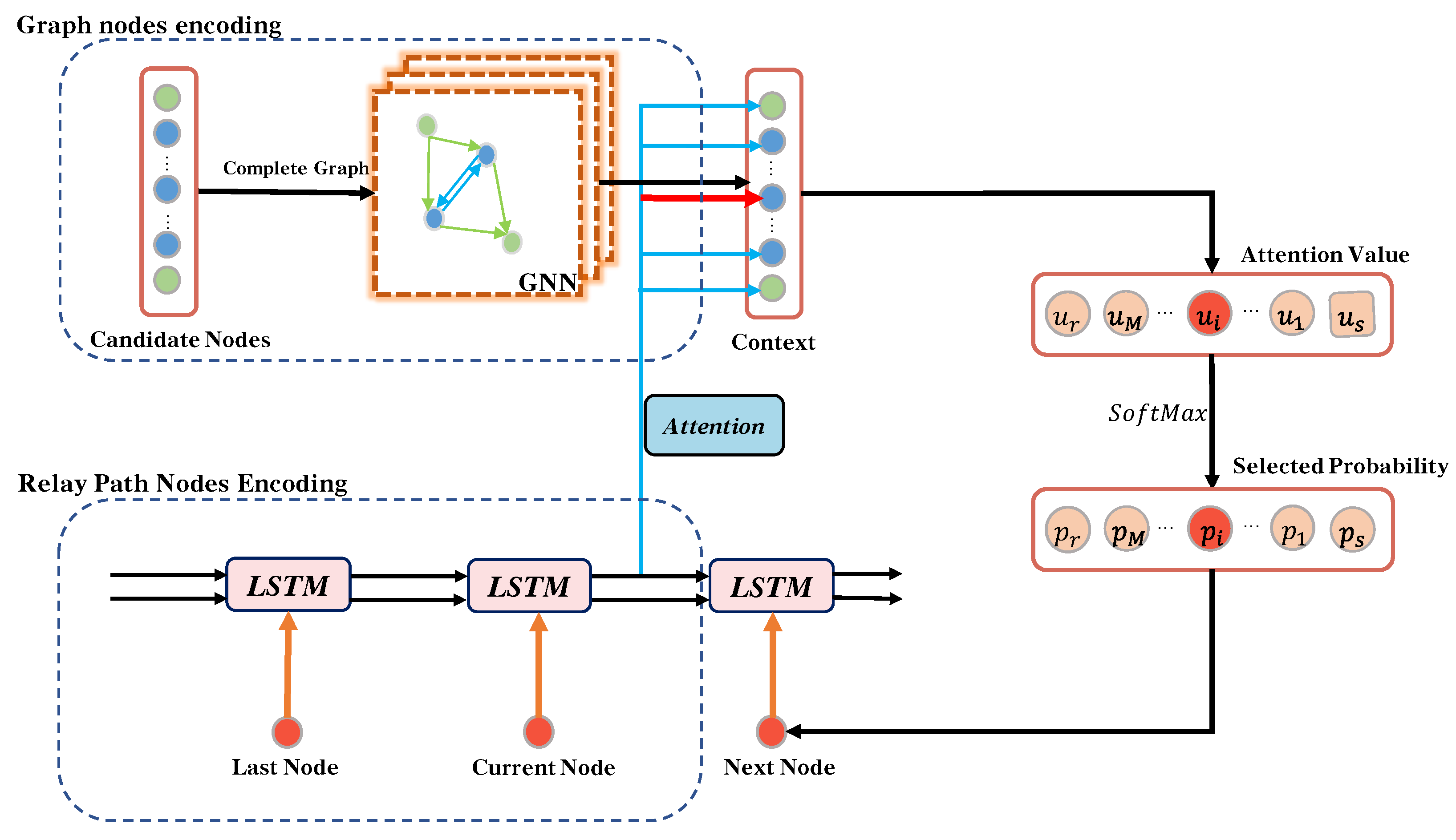
4.2.2. Structure of RGNN

Figure 3 shows the structure of RGNN. It consists of an encoder and a decoder whose details are introduced as follows. The encoder consists of graph nodes encoder to encode the feature of each graph node as a vector, and relay path encoder to encode the feature of the entire relay path as a vector. Then the attention modular is used to compute the influence for each node in graph on the communication rate of relay path, by calculating the value of dot product between relay path encoding vector and all graph node encoded vector. The node has biggest influence on relay path is chosen as the next relay hop.

Encoder: The encoder consists of two parts, i.e., a GNN to extract the features of all nodes, and an LSTM to extract the features of the selected relay path.

Firstly, we use a GNN to embed the information for the feature of each node and the influence of its neighbours on it into a one-dimensional vector [24]. The embedding process for node i in k-th layer of GNN is described as

$$\begin{array}{cc}\hfill & m_{i_r}^k={\varphi }_{\theta }\left(\frac{1}{\left|\mathcal{N}\right(i\left)\right|}{\left\{{\mathbf{x}}_{i_r}^{k-1}\right\}}_{i\in \mathcal{N}\left(i\right)\cup \left\{i\right\}}\right)\hfill \end{array}$$

(27)

$$\begin{array}{cc}\hfill & x_{i_r}^k=\gamma W_1{\mathbf{x}}_{i_r}^{k-1}+(1-\gamma )m_{i_r}^k\hfill \end{array}$$

(28)

where $W_1$ are trainable parameters, $\gamma$ is a factor, and ${\varphi }_{\theta }$ is a trainable aggregating function, and $\mathcal{N}\left(i\right)$ is the neighbor nodes set of node i, and the subscript r is used to denote that this vector is calculated by RGNN. In GNN, we use Equation (27) to process the features from neighbouring nodes and aggregate the features of all neighbouring nodes through the aggregation function ${\varphi }_{\theta }$. Equation (28) is used to process the node i and the features of the aggregated neighbouring nodes. Thus, RGNN embeds the features of node i and its effect on other nodes in the graph into a one-dimensional vector $x_i$.

Figure 3. The Structure of RGNN.

Figure 3. The Structure of RGNN.

Secondly, LSTM is exploited to extract the features of the currently selected relay node. There are two main reasons to use LSTM: (1) relay nodes are sequential, and the previously selected node affects which node should be selected later as the next relay; (2) the LSTM can extract the features of the whole path consisting by the selected nodes, due to its memory capability. The LSTM extracts the features of the current relay link as follows:

$$\begin{array}{c}\hfill h^t,c^t=\mathrm{LSTM}(x_r^t;h^{t-1},c^{t-1})\end{array}$$

(29)

where $h^t$ and $c^t$ are the features of the total selected relay path and the feature of t-th relay node in the relay path respectively, and $x^t$ is the embedded feature of the node which are selected as t-th relay node. In the initial, the feature extracted by GNN for sender $x_{s_r}$ is input to LSTM, and then feature for all relay nodes extracted by GNN are entered into the LSTM in turn.

Decoder: The decoder uses Equation (30) to calculate the attention value for each node in ${\mathcal{V}}_s^{next}$, the higher attention value means the node has more influence on the rate of relay path.

$$\begin{array}{cc}\hfill & p_u^t=\left\{\begin{array}{cc}{\left(h^{t-1}\right)}^{T}tanh(W_2{x}_{v_r}+W_3{h}^{t-1})\hfill & v\in {\mathcal{V}}_s^{next},\hfill \\ -\infty \hfill & otherwise,\hfill \end{array}\right.\hfill \end{array}$$

(30)

where $W_2$ and $W_3$ are trainable parameters, and $tanh(·)$ is hyperbolic tangent function. Then, we use the Softmax function to calculate the selecting probability for each node, and select the node with the highest output value as the next hop, i.e.,

$$\begin{array}{c}\hfill {\pi }_{\theta }(s_t,a_t)=Softmax\left(p_u^t\right),\end{array}$$

(31)

For a node u already in the current path, i.e., $u\in {\mathcal{V}}_s^{selected}$, $p_u^t$ is manually set to $-inf$, avoiding loops in the relay path.

Algorithm 1: Training procedure of LGNN-RGNN method

1:  /* Training RGNN */ 2:  for $train\leftarrow 0$ to $epoch$ do 3:    Randomly generate a graph $\mathcal{G}$ to train RGNN 4:    for s in ${\mathcal{V}}_s$ do 5:      ${\mathcal{G}}_s=\left({\mathcal{V}}_s^{all},{\mathcal{E}}_s\right)$, where ${\mathcal{V}}_s^{all}={\mathcal{V}}_u\bigcup \{s,r\}$, and ${\mathcal{E}}_s$ is the subset of ${\mathcal{E}}_s$ that removes edges formed by nodes not in ${\mathcal{V}}_s^{all}$. 6:      Using RGNN to calculate the embedding vector x for each node in ${\mathcal{G}}_s$ 7:      Initialize the state ${\mathcal{V}}_s^{selected}=\left\{s\right\}$; 8:      for $t\leftarrow 0$ to $|{\mathcal{V}}_u|$ do 9:         if $r\in {\mathcal{V}}_s^{selected}$ then 10:           Break 11:        end if 12:        Calculate the featurte of relay path through Equation (29). 13:        Calculate probability for all nodes in ${\mathcal{V}}_s^{next}$ by Equations (30) and (31). 14:        Select the node with maximum probability as next-hop relay node $n_{next}$. 15:        Update the ${\mathcal{V}}_s^{next}={\mathcal{V}}_s^{next}\backslash \left\{n_{next}\right\}$, ${\mathcal{V}}_s^{selected}={\mathcal{V}}_s^{selected}\bigcup \left\{n_{next}\right\}$ 16:      end for 17:      Calculate the reward of selecting relay path of sender s by Equation (23). 18:    end for 19:    Update the parameters of RGNN by Equations (24) and (26). 20:  end for 21:  /* Training LGNN */ 22:  for $train\leftarrow 0$ to $epoch$ do 23:    Randomly generate a graph $\mathcal{G}$ to train LGNN. 24:    Calculate the location $\mathcal{D}$ of all UAVs by Equations (37)–(42). 25:    Update the parameters of LGNN by Equation (36). 26:  end for

Algorithm 2: Inference procedure of LGNN-RGNN method

1: Input the graph $\mathcal{G}$ to LGNN to optimize the location $\mathcal{D}$ of UAVs by Equations (37)–(42). 2: Move all UAVs to the new location according to $\mathcal{D}$. 3: fors in ${\mathcal{V}}_s$ do 4:    Calculate the relay path for sender s using RGNN based on the new location $\mathcal{D}$ of UAVs. 5: end for

Theorem 1. 

The complexity of the BF-based best relay path selecting algorithm is two orders higher than the RGNN-based method.

Proof. 

According to [55], the complexity of finding the best relay path for one pair of users is $\mathcal{O}\left(n^3\right)$ using BF, where n is the number of relay nodes, i.e., $n=|{\mathcal{V}}_u|$. Since there are $|{\mathcal{V}}_s|$ pairs of users, the BF algorithm is executed $|{\mathcal{V}}_s|$ times, and therefore the total complexity of BF is $\mathcal{O}\left(\right|{\mathcal{V}}_s\left|\right|{\mathcal{V}}_u{|}^3)$. Since the RGNN removes each next-hop node from the set of optional nodes when selecting a relay link, the RGNN removes that node from the set ${\mathcal{V}}_s^{next}$ of optional nodes. Therefore, RGNN will find a relay path by traversing all the elements in the set of optional nodes ${\mathcal{V}}_s^{next}$ at most. In initial state, the $|{\mathcal{V}}_s^{next}| = |{\mathcal{V}}_u|$, since there are $\mathcal{O}\left(\right|{\mathcal{V}}_s\left|\right)$ pairs of users, the complexity of RL-based RGNN is $\mathcal{O}\left(\right|{\mathcal{V}}_s\left|\right|{\mathcal{V}}_u\left|\right)$. Consequently, the time complexity of the BF-based best relay path selecting algorithm is two orders higher than the RGNN-based method. □

4.3. LGNN Based UAV Location Optimization

4.3.1. Unsupervised Learning-Based LGNN Training Method

Recent research has proved that supervised learning methods can train neural networks to solve optimization problems. However, it is necessary to know the problem’s optimal solution as labeled training data, which is unsuitable for solving the UAV location optimization problem. When the number of UAVs and users is large, it is difficult to find a feasible algorithm to solve the problem to produce labeled data. Plus, the robustness of supervised learning is usually poorer than unsupervised and reinforcement learning [57]. Fortunately, since the objective function (17) is differentiable, and the LGNN outputs the locations of all UAVs simultaneously, the RL-based training method in Equation (26) is unnecessary. Therefore, this paper uses unsupervised learning-based methods to train LGNN, which does not need labeled data and has high robustness. Firstly, the derivative of the LGNN output $\mathcal{D}$ concerning the objective function (17) is calculated, and then by the chain rule, the derivative of the LGNN parameters ${\theta }_{LGNN}$ concerning $\mathcal{D}$ can be obtained by following equation. Firstly, according to Problem 1, the objective value is determined by $\mathcal{D}$ and $\mathcal{X}$, thus we rewrite the objective function as

$$\begin{array}{c}\hfill \mathcal{J}(\mathcal{D},\mathcal{X}|\mathcal{G})=\sum _{s\in {\mathcal{V}}_s}\sum _{u\in {\mathcal{V}}_u}{f}_s^{su}.\end{array}$$

(32)

The derivative of the objective function concerning $\mathcal{D}$ is

$$\begin{array}{c}\hfill {\nabla }_{\mathcal{D}}\mathcal{J}(\mathcal{D},\mathcal{X}|\mathcal{G})={\nabla }_{\mathcal{D}}\sum _{s\in {\mathcal{V}}_s}\sum _{u\in {\mathcal{V}}_u}{f}_s^{su}.\end{array}$$

(33)

Since the location of UAVs is determined by LGNN, the $\mathcal{D}$ in this paper is obtained by

$$\begin{array}{c}\hfill \mathcal{D}=LGN{N}_{\theta }\left(\mathcal{G}\right).\end{array}$$

(34)

By replacing the $\mathcal{D}$ is Equation (33) as Equation (34), and calculating the derivative of $\mathcal{D}$ concerning ${\theta }_{LGNN}$, we can get the derivative of objective function concerning ${\theta }_{LGNN}$ as

$$\begin{array}{c}\hfill {\nabla }_{{\theta }_{LGNN}}\mathcal{J}(LGN{N}_{\theta }\left(\mathcal{G}\right),\mathcal{X}|\mathcal{G})={\nabla }_{\mathcal{D}}{\mathcal{J}(\mathcal{D},\mathcal{X}|\mathcal{G})|}_{\mathcal{D}=LGNN\left(\mathcal{G}\right),\mathcal{X}=RGNN\left(\mathcal{G}\right)}{\nabla }_{{\theta }_{LGNN}}LGN{N}_{\theta }\left(\mathcal{G}\right),\\ \hspace{1em}\hspace{1em}\hspace{1em}\hspace{1em}\hspace{1em}\hspace{1em}\hspace{1em}\hspace{1em}\hspace{1em}\hspace{1em}\hspace{1em}={\nabla }_{\mathcal{D}}\sum _{s\in {\mathcal{V}}_s}\sum _{u\in {\mathcal{V}}_u}{f}_s^{su}{|}_{\mathcal{D}=LGNN\left(\mathcal{G}\right),\mathcal{X}=RGNN\left(\mathcal{G}\right)}{\nabla }_{{\theta }_{LGNN}}LGN{N}_{\theta }\left(\mathcal{G}\right).\end{array}$$

(35)

Thus, we can update the ${\theta }_{LGNN}$ by gradient descent as

$$\begin{array}{c}\hfill {\theta }_{LGNN}={\theta }_{LGNN}+{\mu }_L{\nabla }_{\mathcal{D}}\sum _{s\in {\mathcal{V}}_s}\sum _{u\in {\mathcal{V}}_u}{f}_s^{su}{|}_{\mathcal{D}=LGNN\left(\mathcal{G}\right),\mathcal{X}=RGNN\left(\mathcal{G}\right)}{\nabla }_{{\theta }_{LGNN}}LGN{N}_{\theta }\left(\mathcal{G}\right),\end{array}$$

(36)

where ${\mu }_L$ is the learning rate to update LGNN, ${\nabla }_{\mathcal{D}}{\sum }_{s\in {\mathcal{V}}_s}{\sum }_{u\in {\mathcal{V}}_u}{f}_s^{su}{|}_{\mathcal{D}=LGNN\left(\mathcal{G}\right),\mathcal{X}=RGNN\left(\mathcal{G}\right)}$ is the gradient of LGNN’s output $\mathcal{D}$, and ${\nabla }_{{\theta }_{LGNN}}LGN{N}_{\theta }\left(\mathcal{G}\right)$ is the gradient derived by chain rule to update all parameters in LGNN.

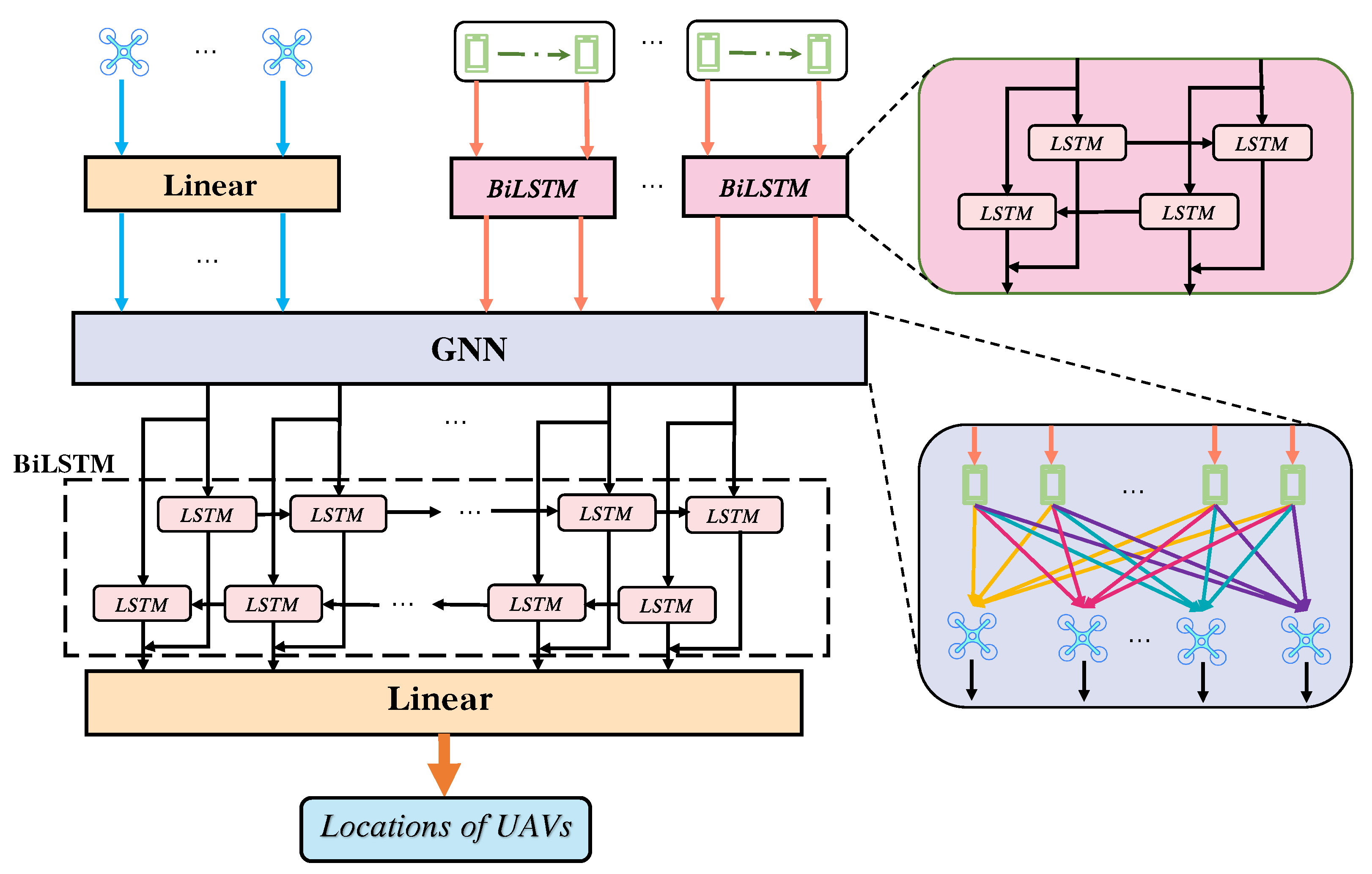
4.3.2. Structure of LGNN

Since LGNN aims to maximize the communication rate for all pairs of users, it is essential to know which two users need to communicate with each other. A naive method is adding a flag to the feature of each user; the users with the same flag mean there is communication demand. However, it has poor performance since it is challenging for LGNN to learn the flag’s meaning. Therefore, as is shown in Figure 4, we propose an LSTM-based method to solve this problem. In this method, the features of two users with communication demand are entered into the LSTM as a sequence with length 2, and the output of the LSTM is used as the embedded feature for each user. Since the LSTM only inputs the feature of two users at a time, the LGNN can know which two users have communication demands while calculating the gradient. This is because only the information of these two users has an interrelationship, and the other users are independent of these two users in calculating the gradient.

After embedding the feature of all users, a GNN is used to extract the relationships among users and UAVs, such that UAVs can optimize their location based on their initial location and the location of all users. Obviously, the optimized locations of each UAV should be close to the initial location, and different users should have different impacts on UAVs, which means users closer to the UAV have a more significant impact on it. Therefore, we use the attention method to calculate the impact of different users on UAVs. Details of the process of LGNN are as follows.

$$\begin{array}{cc}\hfill & m_{i_l,j_l}={\mathrm{MLP}}_1(x_{i_l},x_{j_l}),(i,j)\in \mathcal{E},\hfill \end{array}$$

(37)

$$\begin{array}{cc}\hfill & x_{i_l}={\mathrm{MLP}}_2(x_{i_l},\rho \{{\alpha }_{ij}{m}_{i_l,j_l}:(i,j)\in \mathcal{E}\}),\hfill \end{array}$$

(38)

$$\begin{array}{cc}\hfill & {\alpha }_{ij}=\frac{exp\left(\mathrm{LeaklyReLu}\left(\left[W_4{x}_{i_l}\left|\right|W_5{x}_{j_l}\right]\right)\right)}{{\sum }_{k\in \mathcal{N}\left(i\right)}exp\left(\mathrm{LeaklyReLu}\left(\left[W_4{x}_{i_l}\left|\right|W_5{x}_{k_l}\right]\right)\right)},\hfill \end{array}$$

(39)

$$\begin{array}{cc}\hfill & \mathrm{LeaklyReLu}\left(x\right)=\left\{\begin{array}{cc}x\hfill & x\le 0,\hfill \\ ϵx\hfill & otherwise,\hfill \end{array}\right.\hfill \end{array}$$

(40)

$$\begin{array}{cc}\hfill & x_{i_b}=\mathrm{concat}({\mathrm{LSTM}}_1\left(x_{i_l}\right),{\mathrm{LSTM}}_2\left(x_{i_l}\right)),\hfill \end{array}$$

(41)

$$\begin{array}{cc}\hfill & d_i=W_6{x}_{i_b},\hfill \end{array}$$

(42)

where $W_4$, $W_5$ and $W_6$ are trainable parameters, and $ϵ$ is a factor much more minor than 1. $\rho (·)$ is the aggregation function, and the function concat$(·)$ is used to concatenate the output of ${\mathrm{LSTM}}_1$ and ${\mathrm{LSTM}}_2$ into a vector $x_{i_b}$. The ${\mathrm{LSTM}}_1$ and ${\mathrm{LSTM}}_2$ are two LSTMs with opposite directions, and $d_i$ is the optimized position of UAV i. Equation (37) is used to process the information from neighbour nodes and the LGNN uses Equation (38) to extract the feature both from itself and aggregated feature from neighbors. Equation (39) are used to calculate the impact of different users on UAVs. Since there are multiple UAVs in the system, they should cooperate to optimize the overall performance. Therefore, we further use a bi-directional LSTM (BiLSTM) in Equation (41) to process the feature of UAVs extracted by GNN, such that the position of each UAV can impact other UAVs. Finally, in Equation (42) trainable parameters $W_6$ are used to process the output of BiLSTM, and the $d_i$ is taken as the optimized position of UAV i.

5. Performance Evaluation and Discussion

In this section, we conduct extensive simulations to evaluate our proposed LGNN-RGNN, comparing it with the genetic algorithm (GA), MLP, and Bellman-Ford algorithm. We mainly use the two metrics, “communication rate” and “computation time”, to show the characteristics of different algorithms. The communication rate is to show the average communication rate for all pairs of user, which is same as the value of objective function in Equation (17), and the computation time is to show the running time for different algorithms to get the optimized location of UAV and relay path for each pair of users. We take the genetic algorithm and MLP as the benchmarks for location model LGNN, and Bellman-Ford algorithm is taken as the benchmark for relay path searching model RGNN.

The benchmarks for comparison are as follows.

• LGNN-BF: In this scheme, the proposed LGNN is used to optimize the UAV-relay locations. However, the Bellman-Ford (BF) algorithm is used for relay path selection. The loss of LGNN is set as the opposite of the average Rate of relay paths calculated by BF algorithm.
• GA-RGNN: GA is used to optimize the locations of UAVs. GA generates a large population. Every individual in the population includes all the locations of UAVs. The fitness of individuals is set to the rate output from RGNN. In every iteration, the selection operator is used to keep individuals with higher rate alive and disuse other individuals with low rate. The crossover operator and mutation operator are applied to generate new individuals. The mutation rate of GA is set to 0.2, the scale of population is set as 100 and the multi-point crossover is taken as the crossover operator. The deterministic selection is taken as the selection operator to ensure the best individual could be kept and the top 30 percent of individuals are kept by GA while the left 70 percent individuals can be kept with a 0.3 probability.
• GA-BF: GA is set to optimize the locations of UAVs and the commucation rate output from Bellman-Ford algorithm is set as the fitness of individuals.
• MLP-RGNN: A MLP takes users’ locations as the input, indicating that the number of nodes in input layers is two times the number of users. There is one hidden layer with 128 nodes. The MLP outputs the locations of all UAVs in the output layer. ReLU is used as the activation function of the hidden layer. The opposite of the average rate calculated by RGNN is used as the loss value. The learning rate of MLP is 1e-4.
• MLP-BF: The hyper-parameters of MLP are the same as MLP-RGNN. Loss is set to the opposite of average rate calculated by the BF algorithm.

5.1. Simulation Configurations

In experiments, we evaluate the performance of the proposed method with the different number of users and UAVs. In the training and testing procedure, the users are randomly distributed by uniform distribution from 0 to the maximum length of the network area. In the simulation, the sender randomly chooses one receiver to communicate with the same probability. Obviously, when there are $|{\mathcal{V}}_u|$ UAVs in the network, the maximum network area can be covered is $2|{\mathcal{V}}_u|{\xi }^2\pi$. Therefore, we consider the network as a square area with side length $\xi \sqrt{2|{\mathcal{V}}_u|\pi }$. The communication coverage $\xi$ is $5.0$ km. The bandwidth B is 500 kHz. More simulation parameters in the training procedure are shown in

Table 1. Simulation Parameters in the training procedure.

Parameter Definition	Notation	Value
Number of User Pairs in small-scale network	K (or $|{\mathcal{V}}_s|$)	[2, 20]
Number of User Pairs in large-scale network	K (or $|{\mathcal{V}}_s|$)	[50, 250]
Number of UAVs in small-scale network	M (or $|{\mathcal{V}}_u|$)	[2, 10]
Number of UAVs in large-scale network	M (or $|{\mathcal{V}}_u|$)	[10, 35]
Network area in small-scale network	∖	[100, 500] $\pi$ km2
Network area in large-scale network	∖	[500, 1750] $\pi$ km2
Learning rate of RGNN	${\mu }_{RGNN}$	0.001
Learning rate of LGNN	${\mu }_{LGNN}$	0.0001
Transmission Power	P	0.1 w
Noise Power	$N_0$	−174 dBm/Hz
Path-loss constant	$g_0$	−40 dB
Path-loss exponent	$\gamma$	2
UAV communication coverage range	$\xi$	5.0 km

. Remarkably, B, P, $N_0$, and $g_0$ are always the same in the network of any scale, both in training and testing procedures. The central self-critic baseline is used during the training process. The update of parameters of RGNN is based on Policy gradient descent according to Equation (26). The communication requirements between users are also generated randomly. RGNN model uses a three-layer GNN in Encoder, where every layer of GNN is set as in Equation (28). The message passing function is a two-layer MLP with ReLU as the activation function, and the dimension of hidden layer is 128. The update function is also a two-layer MLP, with the dimension of the hidden layer being 128. The aggregation function $\rho$ is the average function $mean$. In the training procedure, we first train the RGNN with the random location of UAVs and users, and the communication requirements among users are also randomly generated. With the trained RGNN offering the relay path of each pair of users, we pre-train our proposed LGNN according to Equation (36). To prevent overfitting, LGNN is pre-trained on samples with different scales. In each sample, the number of UAVs is selected randomly from the range of 2–20, while the number of user pairs is randomly selected from the range of 5–100. We pre-train LGNN with 4096 samples.

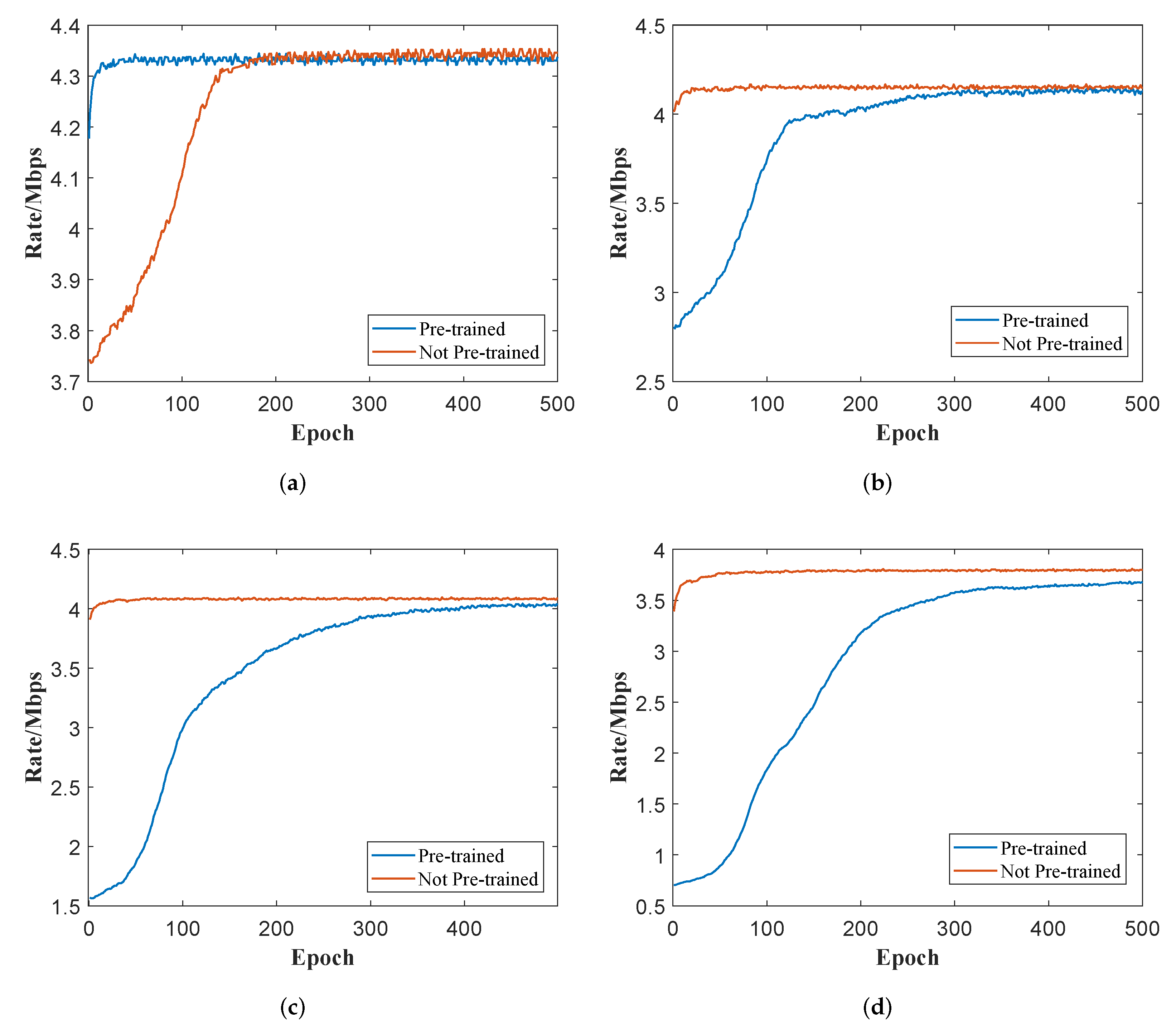
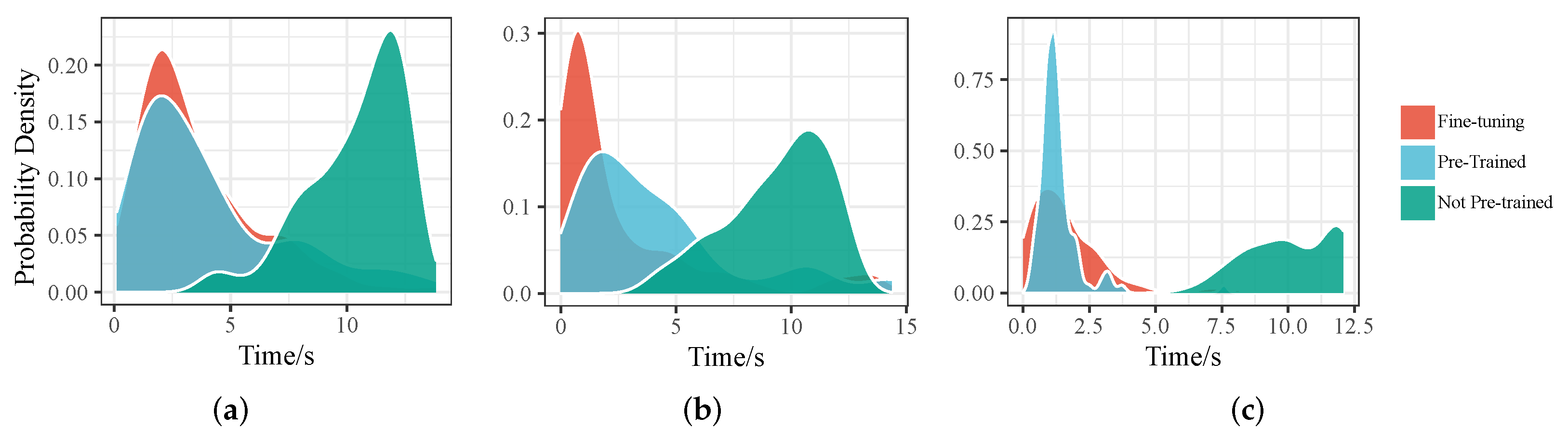
5.2. Performance of Pre-Trained RGNN and LGNN

The BF Algorithm is taken as the baseline, providing the best relay path for every user. We evaluate the performance of trained RGNN by comparing it with BF Algorithm. The hyper-parameters of training process of RGNN is discussed in Section 5.1. In testing data, we set $|{\mathcal{V}}_s|=4|{\mathcal{V}}_u|$. Figure 5 shows the communication rate and computation time for RGNN and BF algorithm. For GNN-based methods, the computation time in this paper includes the training or fine-tuning time plus inference time, while for GA-based methods the computation time is the algorithm execution time via iterations until certain finishing conditions are met. According to Figure 5a, the RGNN achieves very close performance to the BF algorithm when $|{\mathcal{V}}_u|$ is lower than 8, which means that when the network is not too large, the RGNN can find the best relay path. However, the optional relay paths for each pair of users are proportional to the factorial of $|{\mathcal{V}}_u|$. Therefore, the RGNN may not be able to select the optimal relay path when $|{\mathcal{V}}_u|$ is large. Figure 5b shows that as $|{\mathcal{V}}_u|$ increases, the computation time of BF algorithm increases dramatically while that of RGNN only arises a little. This is because not only the time complexity of RGNN is two orders lower than BF, but also the RGNN can use graphics processing unit (GPU) to compute in parallel while BF cannot.

According to [58], pre-training is a useful method to improve convergence speed and even convergence performance. Therefore, in this paper, we randomly generate many graphs with different scales to pre-train LGNN. Figure 6 shows the performance of pre-trained LGNN and non-pre-trained LGNN. It can be seen that the initial performance of pre-trained LGNN consistently outperforms the performance of non-pre-trained LGNN by a wide margin across all sizes of networks. This means that pre-training allows the LGNN to learn generalised features of the network, thus improving zero-shot performance and allowing the network to converge to a good performance quickly, which is specifically beneficial for changing environments and services sensitive to delay performance. It also shows the pre-trained LGNN can get better convergence performance than non-pre-trained LGNN. Therefore, in the following paper, if not specified, the LGNN denotes pre-trained LGNN.

5.3. Optimality Analysis of the Proposed LGNN-RGNN Approach

To analyze whether our proposed algorithm achieves near-optimal performance, we compare the proposed LGNN-RGNN method with the brute-force search method and a greedy algorithm. In brute-force search, we discretize the locations of the UAVs into a 20 ∗ 20 grid, and each UAV can be placed in any grid. Iterate through all possible UAVs location, and the BF algorithm is used to calculate the best performance for the current placement using the best relay path. The location of UAVs that achieves the best network performance is recorded as the optimal solution. A greedy algorithm is also used that clusters all users and places the UAVs in the center of the cluster. Simulation results in terms of UAV locations are shown in Figure 7, the horizontal and vertical coordinate values represent the coordinate positions of the user and the UAV in the plane, respectively. In all these four sub-figures the location optimized by greedy algorithm is always far away from the location optimized by brute-force and proposed method, and the performance of greedy method is always the worst. Because the communication rate between two nodes is not proportional to the distance between two nodes, thus it is not the optimal solution to deploy UAVs at the center of user cluster. In Figure 7a the performance of proposed LGNN-RGNN method is a little lower than brute-force, this is because in Figure 7a the distribution of users is dense, when the location of the UAV deviates from the optimal location, it can lead to a significant change in overall performance due to the concentration of users in a few specific areas. Similarly, in in Figure 7b since the distribution of user locations is more dispersed, even if the location of the UAV deviates from the optimal location, the overall performance of the system will be almost unaffected due to the influence of different users. Remarkably, in Figure 7c,d shows when both LGNN-RGNN and brute-force methods output locations near the actual optimal location, LGNN-RGNN may obtain better performance since LGNN outputs the deployment location of the UAV as a continuous value, while the brute-force can only output discrete values.

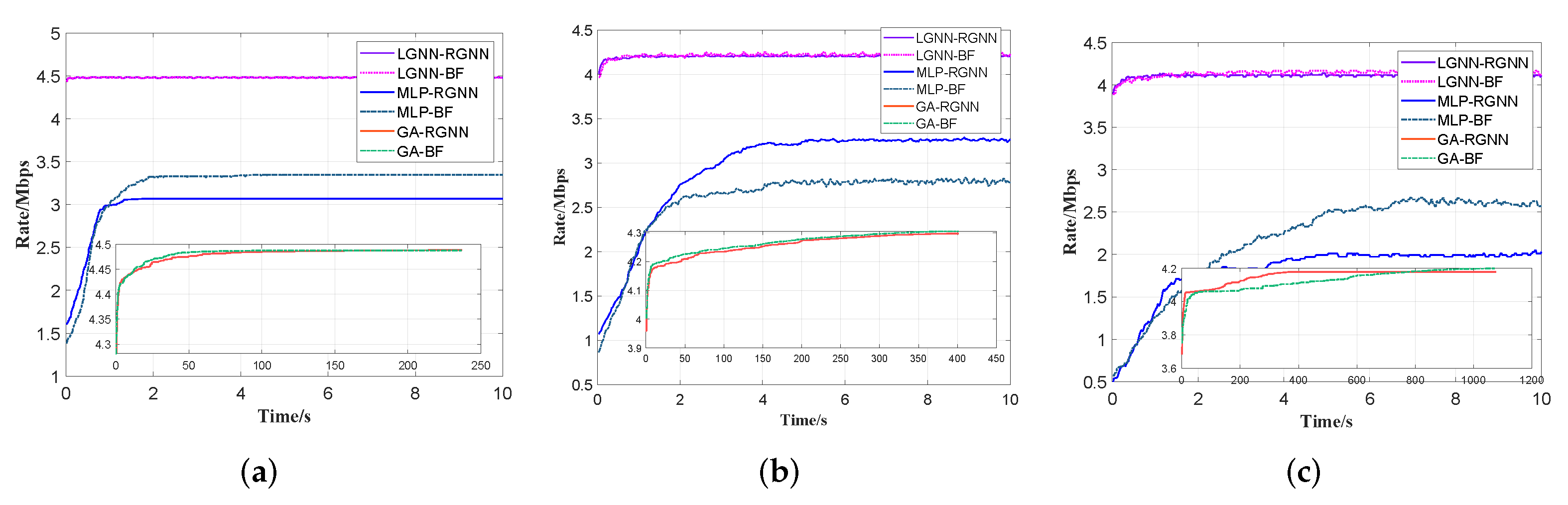
5.4. Convergence Speed and Performance

In Figure 8, we show the convergence speed and communication rate for the different algorithms with the different $|{\mathcal{V}}_s|$ and $|{\mathcal{V}}_u|$. We test the performance of six different algorithms. Because the convergence time of GA-based algorithms is far longer than others, we demonstrate it in a separate figure. The GA-based methods are used as the near-optimal solution since, after sufficient time iterations, the GA can get a locally optimal solution [59]. Figure 8 shows that the proposed LGNN-based algorithms achieve near-optimal performance when the number of users and UAVs is not very large, with a high convergence speed due to pre-training. The LGNN-BF has a higher convergence speed than LGNN-RGNN in a small-scale networks but has lower convergence speed in a large-scale networks. This is because the BF algorithm can always get the optimal relay path, and thus when the scale of the network is small, it can quickly give an accurate gradient to update ${\theta }_{LGNN}$ according to Equation (36), rendering the LGNN converge quickly. However, due to the high computational complexity of the BF algorithm, Figure 8c shows LGNN-BF converges slower than LGNN-RGNN in large-scale networks, mainly due to the computation time of BF itself. Figure 8 also shows that MLP has low convergence speed and ill convergence performance. This is because MLP only tasks all the features of users and UAVs as input without any analysis of the relation of features, therefore, it has low feature extraction ability and poor performance.

5.5. Relation of $|{\mathcal{V}}_s|$ and $|{\mathcal{V}}_u|$ on Performance

Figure 9 shows the impact of $|{\mathcal{V}}_s|$ on communication rate and computation time with $|{\mathcal{V}}_u|=4$. Figure 9a shows that as the number of users increases, the performance of the LGNN-based approach gradually decreases. This is because the increase in the number of users makes the network have more complex connection relationships, and therefore the LGNN confronts greater difficulty in extracting the relationships between users, resulting in a decrease in performance. As the MLP can hardly extract the relationships among users, an increase in the number of users has no significant impact on the MLP the overall performance is oscillatory. As for the computation time, Figure 9b shows the BF-based algorithm increasing faster than the RGNN-based method since the RGNN can compute in parallel using GPU while BF cannot. Moreover, the LGNN-based method has a faster computational speed since LGNN has much fewer parameters than MLP.

Figure 10 shows the impact of $|{\mathcal{V}}_u|$ on communication rate and computation time with $|{\mathcal{V}}_s|=20$. Figure 10a shows that as $|{\mathcal{V}}_u|$ increases, the performance of all algorithms increases since increasing $|{\mathcal{V}}_u|$ reduces the average distance between UAVs and UAVs and between UAVs and users, thus improving the network communication rate. LGNN-based methods increase faster than MLP-based methods since LGNN can extract the relation among UAVs and thus get better performance. As is shown in Figure 5a, when the number of UAVs is large, the performance of RGNN is lower than BF. Therefore, in Figure 10a, when $|{\mathcal{V}}_u|$ is large, the performance of the BF-based method is higher than the RGNN-based method. Thus, the LGNN and MLP obtain the incorrect update gradient according to Equation (36), which degrades the performance of the LGNN and MLP. Figure 10b shows that LGNN-based methods always compute faster than MLP-based methods due to fewer parameters. Moreover, the computation time of BF-based methods increases much more dramatically than RGNN-based methods. This is because when $|{\mathcal{V}}_u|$ is constant, the time complexity of BF is two orders higher than that of RGNN according to Theorem 1. Therefore, we can choose relay path selecting methods based on preference on time and performance.

Both Figure 9a and Figure 10a show that the $|{\mathcal{V}}_u|$ has more impact on communication rate than $|{\mathcal{V}}_s|$, mainly due to the relay path selection. When $|{\mathcal{V}}_u|$ increases, the average distance between UAV and user decreases; thus the average rate for all optional relay paths increases. However, since each pair of user selects their relay path, the average communication rate for all users changes little with constant $|{\mathcal{V}}_u|$.

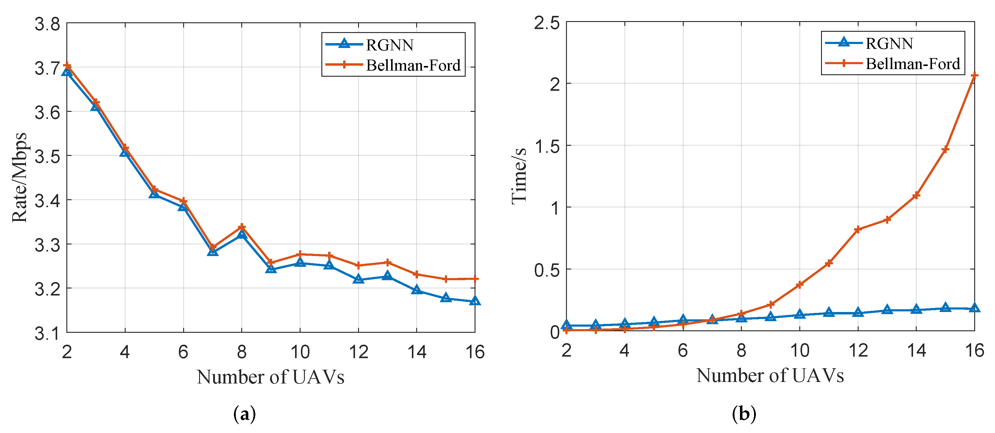
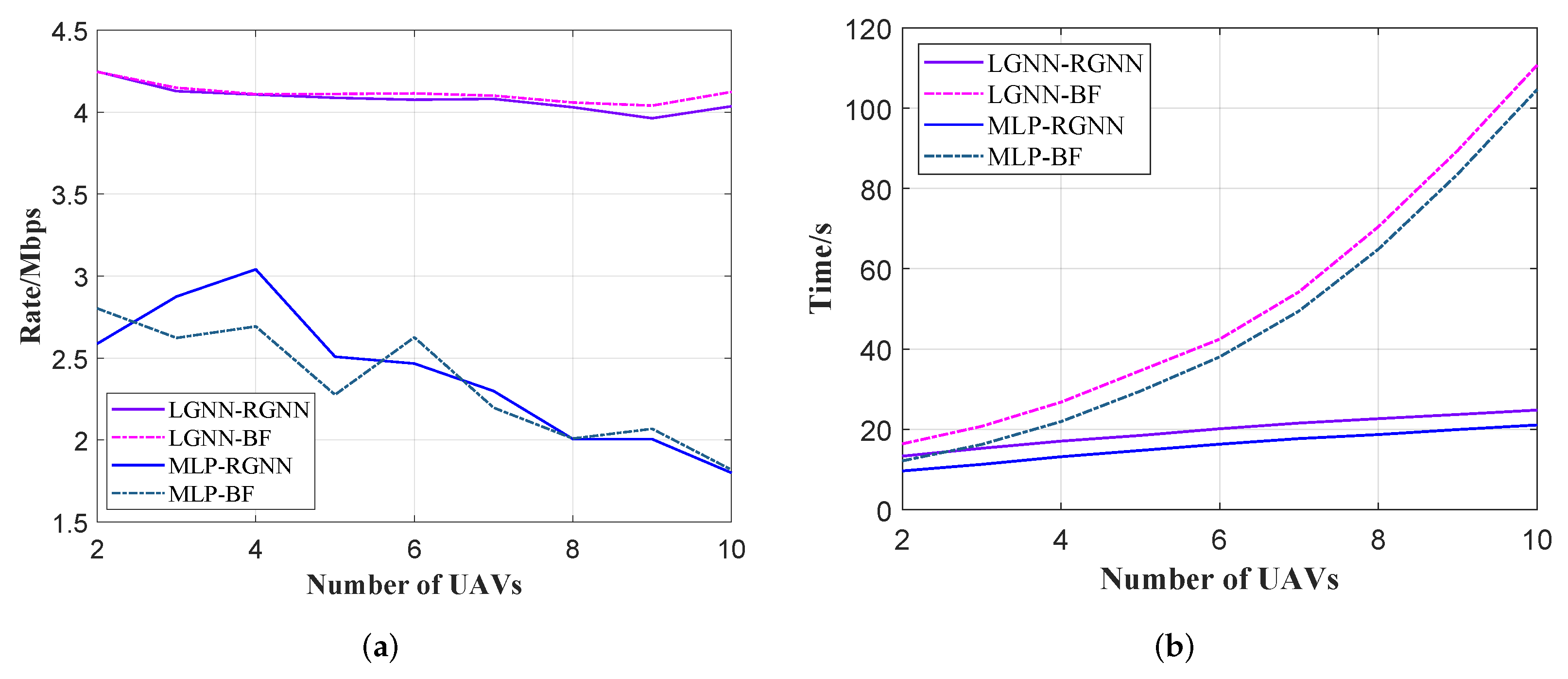
5.6. Performance in Large-Scale Networks

Scalability is a critical consideration since many algorithms cannot fit the large-scale problems due to poor performance or unacceptably long solving time. In this part, we evaluate the performance of the proposed method on a large-scale network, and the results are shown in

Table 2. Performance on a large-scale network for different algorithms.

(a) Performance on$|{\mathcal{V}}_{\mathit{s}}|=\mathbf{50}$$|{\mathcal{V}}_{\mathit{u}}|=\mathbf{15}$for Different Algorithms			(b) Performance on$|{\mathcal{V}}_{\mathit{s}}|=\mathbf{100}$$|{\mathcal{V}}_{\mathit{u}}|=\mathbf{20}$for Different Algorithms
Algorithms	Rate/Mbps	Computation Time/s	Algorithms	Rate/Mbps	Computation Time/s
MLP	2.24	10.59	MLP	2.31	20.03
Greedy	3.03	0.09	Greedy	3.00	0.13
LGNN-RGNN (DI)	3.79	0.05	LGNN-RGNN (DI)	3.44	0.06
LGNN-RGNN (FT)	3.88	7.98	LGNN-RGNN (FT)	3.65	15.72
(c) Performance on$|{\mathcal{V}}_{\mathbf{s}}|=\mathbf{150}$$|{\mathcal{V}}_{\mathbf{u}}|=\mathbf{25}$for Different Algorithms			(d) Performance on$|{\mathcal{V}}_{\mathbf{s}}|=\mathbf{250}$$|{\mathcal{V}}_{\mathbf{u}}|=\mathbf{35}$for Different Algorithms
Algorithms	Rate/Mbps	Computation Time/s	Algorithms	Rate/Mbps	Computation Time/s
MLP	2.15	21.88	MLP	1.71	48.68
Greedy	2.67	0.17	Greedy	2.36	0.22
LGNN-RGNN (DI)	3.22	0.08	LGNN-RGNN (DI)	3.02	0.15
LGNN-RGNN (FT)	3.43	15.73	LGNN-RGNN (FT)	3.18	44.79

. We conduct this experiment in four different large-scale networks. Besides, we pre-trained LGNN and RGNN with large-scale samples to improve the performance of proposed LGNN-RGNN. RGNN is pre-trained with each sample having 20 nodes including 18 UAVs and 2 IoTs. LGNN is pre-trained with 4096 samples. In each sample, the number of UAVs is selected randomly from the range of 50–350, while the number of user pairs is randomly selected from the range of 10–40. According to the analysis and results above, the GA-based and BF-based methods cost much time to get the solution. Therefore, in a large-scale network, it is impossible for GA-based and BF-based methods to get a solution in an acceptable time range. Thus, we compare the performance of LGNN-based, MLP-based, and greedy methods. “LGNN-RGNN (DI)” means directly using the pre-trained LGNN and RGNN for solution inference without any fine-tuning. Note that with “LGNN-RGNN (FT)”, the pre-trained LGNN and RGNN continue to train a few epochs for better performance. All these four algorithms use RGNN to calculate the best relay path.

Table 2 shows that the fine-tuned LGNN achieves the best performance. The pre-training method helps the LGNN being robust and learning the general features of the problem for optimizing the location of UAVs, while MLP can hardly extract features of the networks to optimize the problem. Therefore, directly using pre-trained LGNN achieves better performance than MLP. Moreover, the above analysis and results show that it is challenging for MLP to optimize the location of UAVs even in small-scale networks. Therefore, in large-scale networks, the performance of MLP is worse than directly using pre-trained LGNN. Moreover, Table 2 shows that LGNN-RGNN (DI) always cost least time, which only costs 0.15 s even there are 200 pairs of users and 35 UAVs, in all these four methods, while only sacrificing little performance compared to LGNN-RGNN (FT). This is because not only the pre-training method helps the LGNN-RGNN being robust to the problem, which enables pre-trained LGNN-RGNN to optimize the problem in large-scale network with high performance, but also the message passing mechanism of the graph network allows when directly using LGNN-RGNN to inference the optimization solution, only a number, which is proportional to ${\mathcal{V}}_u$, of matrix multiplications is needed [25]. Table 2 shows that the LGNN-RGNN (FT) always achieves best performance, while the time of LGNN-RGNN (DI) costs least time by sacrificing little performance. Thus, if the user is delay-sensitive, directly using the pre-trained LGNN-RGNN to inference is the best choice, while the fine-tuned LGNN-RGNN can get the best performance within an acceptable time.

5.7. Performance on Robustness

In practical applications, the environment and service demands may change over time. For example, the mobile sensors result in location changes of communication devices, and the random communication demands may change the number of communication pairs. These changes are generally not significant in a short period of time. The algorithm, therefore, needs to be robust to these small changes. Genetic Algorithm does not have any generalization ability means that it needs to be completely calculated again after any change in the network. In this part, we test the robustness of algorithms with the probability density function of computation time for model with differently initialized parameters to converge and communication rate. We set 4 ways to initialize the parameters of LGNN. The “Fine-tuning” means LGNN-RGNN that inherits the parameters after training convergence in the original network, and fine-tunes in the network after feature changes. The “Pre-trained” means fine-tuning the parameters using general pre-trained network weights. The difference between “Fine-tuning” and “Pre-trained” is the initial parameters. The “Pre-trained” use the parameters trained through general networks as the initial graph, while the “Fine-tuning” uses the parameters trained by the specific network before changing. Therefore, the “Pre-trained” has more general network knowledge, while the “Fine-tuning” focuses on the original unchanged network. The “Not Pre-trained” means randomly initializing the parameters of LGNN, and then training it to convergence. Moreover, the “Directly-Inference” means doing inference directly with the pre-trained model without any updating, and the time required by this way could be relatively ignored.

In Figure 11a, we change the position of $10\%$ of users randomly within a circle of radius $0.2$ centred on its original position, according to a uniform distribution. In Figure 11b, we randomly choose $10\%$ of users and disrupt their connections randomly. In Figure 11c, we randomly increase and decrease the number of users by $10\%$. Figure 11a,b show that the LGNN-RGNN inheriting parameters in the original network need less computation time to converge. The convergence time of the model initialized with the “Fine-tuning” way is more concentrated in the shorter time, and the parameters even do not need to update in some cases. Besides, general pre-trained LGNN-RGNN can also converge quickly. “Fine-tuning” demonstrates robustness to location changes and connection changes, and it is a practical way to initialize parameters of our proposed LGNN-RGNN in practical application scenarios. Figure 11c shows that the two ways of “Fine-tuning” and “Pre-trained” need similar time to converge and the time required by the two ways is concentrated in a short time. Meanwhile, Figure 12 shows that the communication rate converged in the way of “Fine-tuning” concentrated in higher value. Moreover, the communication rate calculated by “Directly-Inference” shows obvious concentration, which further demonstrates the robustness of our proposed LGNN-RGNN is strong. This indicates that when the network features change, the proposed LGNN-RGNN method can quickly adapt to new features and achieves good performance, thus reducing the time required to generate new networking solutions.

6. Conclusions

In this paper, we have investigated the problem of optimizing the location of UAVs and selecting an optimal relay path for each pair of users in IoT networks. We have proposed the RGNN method to choose the best relay path, which has two orders lower time complexity than BF, and proposed the LGNN method to optimize the location of UAVs. To train the GNN efficiently without labeled training data, we have applied reinforcement learning to train RGNN and unsupervised learning to train LGNN. Simulation results have validated the efficiency and robustness of the proposed method, especially in large-scale IoT networks. Our work can offer valuable insights into the importance yet the under-explored field of GNN-driven UAV optimization in large-scale IoT networks. In the future, we will focus on the trajectory design for UAVs in IoT networks using GNN.

References

1. Dang, S.; Amin, O.; Shihada, B.; Alouini, M.S. What should 6G be? Nat. Electron. 2020, 3, 20–29. [Google Scholar] [CrossRef]
2. Alsamhi, S.H.; Ma, O.; Ansari, M.S.; Almalki, F.A. Survey on Collaborative Smart Drones and Internet of Things for Improving Smartness of Smart Cities. IEEE Access 2019, 7, 128125–128152. [Google Scholar] [CrossRef]
3. Alsamhi, S.H.; Shvetsov, A.V.; Kumar, S.; Shvetsova, S.V.; Alhartomi, M.A.; Hawbani, A.; Rajput, N.S.; Srivastava, S.; Saif, A.; Nyangaresi, V.O. UAV Computing-Assisted Search and Rescue Mission Framework for Disaster and Harsh Environment Mitigation. Drones 2022, 6, 154. [Google Scholar] [CrossRef]
4. Cheng, N.; Lyu, F.; Quan, W.; Zhou, C.; He, H.; Shi, W.; Shen, X. Space/Aerial-Assisted Computing Offloading for IoT Applications: A Learning-Based Approach. IEEE J. Sel. Areas Commun. 2019, 37, 1117–1129. [Google Scholar] [CrossRef]
5. Gholami, A.; Torkzaban, N.; Baras, J.S.; Papagianni, C. Joint mobility-aware UAV placement and routing in multi-hop UAV relaying systems. In Proceedings of the International Conference on Ad Hoc Networks, Bari, Italy, 19–21 October 2020; Springer: Berlin/Heidelberg, Germany, 2020; pp. 55–69. [Google Scholar]
6. Zhong, X.; Guo, Y.; Li, N.; Chen, Y. Joint optimization of relay deployment, channel allocation, and relay assignment for UAVs-aided D2D networks. IEEE/ACM Trans. Netw. 2020, 28, 804–817. [Google Scholar] [CrossRef]
7. Alsamhi, S.H.; Ma, O.; Ansari, M.S.; Gupta, S.K. Collaboration of Drone and Internet of Public Safety Things in Smart Cities: An Overview of QoS and Network Performance Optimization. Drones 2019, 3, 13. [Google Scholar] [CrossRef]
8. Zeng, Y.; Zhang, R.; Lim, T.J. Wireless communications with unmanned aerial vehicles: Opportunities and challenges. IEEE Commun. Mag. 2016, 54, 36–42. [Google Scholar] [CrossRef]
9. Yin, Z.; Jia, M.; Cheng, N.; Wang, W.; Lyu, F.; Guo, Q.; Shen, X. UAV-Assisted Physical Layer Security in Multi-Beam Satellite-Enabled Vehicle Communications. IEEE Trans. Intell. Transp. Syst. 2022, 23, 2739–2751. [Google Scholar] [CrossRef]
10. Yin, Z.; Jia, M.; Wang, W.; Cheng, N.; Lyu, F.; Shen, X. Max-min secrecy rate for NOMA-based UAV-assisted communications with protected zone. In Proceedings of the 2019 IEEE Global Communications Conference (GLOBECOM), Waikoloa, HI, USA, 9–13 December 2019; pp. 1–6. [Google Scholar] [CrossRef]
11. Gupta, A.; Sundhan, S.; Gupta, S.K.; Alsamhi, S.; Rashid, M. Collaboration of UAV and HetNet for better QoS: A comparative study. Int. J. Veh. Inf. Commun. Syst. 2020, 5, 309–333. [Google Scholar] [CrossRef]
12. Hou, T.; Liu, Y.; Song, Z.; Sun, X.; Chen, Y. Multiple antenna aided NOMA in UAV networks: A stochastic geometry approach. IEEE Trans. Commun. 2018, 67, 1031–1044. [Google Scholar] [CrossRef]
13. Zhou, C.; Wu, W.; He, H.; Yang, P.; Lyu, F.; Cheng, N.; Shen, X. Deep reinforcement learning for delay-oriented IoT task scheduling in SAGIN. IEEE Trans. Wirel. Commun. 2020, 20, 911–925. [Google Scholar] [CrossRef]
14. Xia, J.Y.; Li, S.; Huang, J.J.; Yang, Z.; Jaimoukha, I.M.; Gündüz, D. Metalearning-Based Alternating Minimization Algorithm for Nonconvex Optimization. IEEE Trans. Neural Netw. Learn. Syst. 2022. [Google Scholar] [CrossRef] [PubMed]
15. Guo, F.; Yu, F.R.; Zhang, H.; Li, X.; Ji, H.; Leung, V.C. Enabling massive IoT toward 6G: A comprehensive survey. IEEE Internet Things J. 2021, 8, 11891–11915. [Google Scholar] [CrossRef]
16. Ghaleb, S.M.; Subramaniam, S.; Zukarnain, Z.A.; Muhammed, A. Mobility management for IoT: A survey. Eurasip J. Wirel. Commun. Netw. 2016, 2016, 1–25. [Google Scholar] [CrossRef]
17. Kandel, I.; Castelli, M. The effect of batch size on the generalizability of the convolutional neural networks on a histopathology dataset. ICT Express 2020, 6, 312–315. [Google Scholar] [CrossRef]
18. Nguyen, D.C.; Ding, M.; Pathirana, P.N.; Seneviratne, A.; Li, J.; Niyato, D.; Dobre, O.; Poor, H.V. 6G Internet of Things: A comprehensive survey. IEEE Internet Things J. 2021, 359–383. [Google Scholar] [CrossRef]
19. Shen, Y.; Shi, Y.; Zhang, J.; Letaief, K.B. Graph neural networks for scalable radio resource management: Architecture design and theoretical analysis. IEEE J. Sel. Areas Commun. 2020, 39, 101–115. [Google Scholar] [CrossRef]
20. Wu, Z.; Pan, S.; Chen, F.; Long, G.; Zhang, C.; Philip, S.Y. A comprehensive survey on graph neural networks. IEEE Trans. Neural Netw. Learn. Syst. 2020, 32, 4–24. [Google Scholar] [CrossRef] [PubMed]
21. Xu, K.; Hu, W.; Leskovec, J.; Jegelka, S. How powerful are graph neural networks? In Proceedings of the 7th International Conference on Learning Representations (ICLR 2019), New Orleans, LA, USA, 6–9 May 2019; pp. 1–17. [Google Scholar]
22. Chen, Z.; Li, L.; Bruna, J. Supervised community detection with line graph neural networks. In Proceedings of the 7th International Conference on Learning Representations (ICLR 2019), New Orleans, LA, USA, 6–9 May 2019; pp. 1–24. [Google Scholar]
23. Lim, J.; Ryu, S.; Park, K.; Choe, Y.J.; Ham, J.; Kim, W.Y. Predicting drug–target interaction using a novel graph neural network with 3D structure-embedded graph representation. J. Chem. Inf. Model. 2019, 59, 3981–3988. [Google Scholar] [CrossRef]
24. Ma, Q.; Ge, S.; He, D.; Thaker, D.; Drori, I. Combinatorial optimization by graph pointer networks and hierarchical reinforcement learning. arXiv 2019, arXiv:1911.04936. [Google Scholar]
25. Shen, Y.; Zhang, J.; Song, S.; Letaief, K.B. Graph neural networks for wireless communications: From theory to practice. arXiv 2022, arXiv:2203.10800. [Google Scholar]
26. He, H.; Kosasihy, A.; Yu, X.; Zhang, J.; Song, S.; Hardjawanay, W.; Letaief, K.B. Graph neural network enhanced approximate message passing for MIMO detection. arXiv 2022, arXiv:2205.10620. [Google Scholar]
27. Wang, H.; Wu, Y.; Min, G.; Miao, W. A graph neural network-based digital twin for network slicing management. IEEE Trans. Ind. Inform. 2020, 18, 1367–1376. [Google Scholar] [CrossRef]
28. Sun, P.; Lan, J.; Li, J.; Guo, Z.; Hu, Y. Combining deep reinforcement learning with graph neural networks for optimal VNF placement. IEEE Commun. Lett. 2020, 25, 176–180. [Google Scholar] [CrossRef]
29. Goodfellow, I.; Bengio, Y.; Courville, A. Deep Learning; MIT Press: Cambridge, MA, USA, 2016. [Google Scholar]
30. Mozaffari, M.; Saad, W.; Bennis, M.; Debbah, M. Drone small cells in the clouds: Design, deployment and performance analysis. In Proceedings of the 2015 IEEE Global Communications Conference (GLOBECOM), San Diego, CA, USA, 6–10 December 2015; pp. 1–6. [Google Scholar] [CrossRef]
31. Saif, A.; Dimyati, K.; Noordin, K.A.; Shah, N.S.M.; Alsamhi, S.; Abdullah, Q. Energy-efficient tethered UAV deployment in B5G for smart environments and disaster recovery. In Proceedings of the 2021 IEEE 1st International Conference on Emerging Smart Technologies and Applications (eSmarTA), 10–12 August 2021; pp. 1–5. [Google Scholar]
32. Galkin, B.; Kibilda, J.; DaSilva, L.A. Deployment of UAV-mounted access points according to spatial user locations in two-tier cellular networks. In Proceedings of the 2016 Wireless Days (WD), Toulouse, France, 23–25 March 2016; pp. 1–6. [Google Scholar] [CrossRef]
33. Huang, H.; Savkin, A.V. Reactive deployment of flying robot base station over disaster areas. In Proceedings of the 2018 IEEE International Conference on Robotics and Biomimetics (ROBIO), Kuala Lumpur, Malaysia, 12–15 December 2018; pp. 1665–1670. [Google Scholar] [CrossRef]
34. Huang, H.; Savkin, A.V. A Method for Optimized Deployment of Unmanned Aerial Vehicles for Maximum Coverage and Minimum Interference in Cellular Networks. IEEE Trans. Ind. Inform. 2019, 15, 2638–2647. [Google Scholar] [CrossRef]
35. Cicek, C.T.; Gultekin, H.; Tavli, B.; Yanikomeroglu, H. UAV base station location optimization for next generation wireless networks: Overview and future research directions. In Proceedings of the 2019 1st International Conference on Unmanned Vehicle Systems-Oman (UVS), Muscat, Oman, 5–7 February 2019; pp. 1–6. [Google Scholar] [CrossRef]
36. Sabzehali, J.; Shah, V.K.; Fan, Q.; Choudhury, B.; Liu, L.; Reed, J.H. Optimizing Number, Placement, and Backhaul Connectivity of Multi-UAV Networks. IEEE Internet Things J. 2022, 1. [Google Scholar] [CrossRef]
37. Kang, Z.; You, C.; Zhang, R. Placement learning for multi-UAV relaying: A Gibbs sampling approach. In Proceedings of the ICC 2020–2020 IEEE International Conference on Communications (ICC), Dublin, Ireland, 7–11 June 2020; pp. 1–6. [Google Scholar] [CrossRef]
38. Košmerl, J.; Vilhar, A. Base stations placement optimization in wireless networks for emergency communications. In Proceedings of the 2014 IEEE International Conference on Communications Workshops (ICC), Sydney, Australia, 10–14 June 2014; pp. 200–205. [Google Scholar] [CrossRef]
39. Kalantari, E.; Yanikomeroglu, H.; Yongacoglu, A. On the number and 3D placement of drone base stations in wireless cellular networks. In Proceedings of the 2016 IEEE 84th Vehicular Technology Conference (VTC-Fall), Montreal, QC, Canada, 18–21 September 2016; pp. 1–6. [Google Scholar] [CrossRef]
40. Plachy, J.; Becvar, Z.; Mach, P.; Marik, R.; Vondra, M. Joint Positioning of Flying Base Stations and Association of Users: Evolutionary-Based Approach. IEEE Access 2019, 7, 11454–11463. [Google Scholar] [CrossRef]
41. Alsamhi, S.H.; Shvetsov, A.V.; Kumar, S.; Hassan, J.; Alhartomi, M.A.; Shvetsova, S.V.; Sahal, R.; Hawbani, A. Computing in the Sky: A Survey on Intelligent Ubiquitous Computing for UAV-Assisted 6G Networks and Industry 4.0/5.0. Drones 2022, 6, 177. [Google Scholar] [CrossRef]
42. Chaudhri, S.N.; Rajput, N.S.; Alsamhi, S.H.; Shvetsov, A.V.; Almalki, F.A. Zero-padding and spatial augmentation-based gas sensor node optimization approach in resource-constrained 6G-IoT paradigm. Sensors 2022, 22, 3039. [Google Scholar] [CrossRef]
43. Salh, A.; Audah, L.; Alhartomi, M.A.; Kim, K.S.; Alsamhi, S.H.; Almalki, F.A.; Abdullah, Q.; Saif, A.; Algethami, H. Smart Packet Transmission Scheduling in Cognitive IoT Systems: DDQN Based Approach. IEEE Access 2022, 10, 50023–50036. [Google Scholar] [CrossRef]
44. Scarselli, F.; Gori, M.; Tsoi, A.C.; Hagenbuchner, M.; Monfardini, G. The Graph Neural Network Model. IEEE Trans. Neural Netw. 2009, 20, 61–80. [Google Scholar] [CrossRef] [PubMed]
45. Greff, K.; Srivastava, R.K.; Koutník, J.; Steunebrink, B.R.; Schmidhuber, J. LSTM: A Search Space Odyssey. IEEE Trans. Neural Netw. Learn. Syst. 2017, 28, 2222–2232. [Google Scholar] [CrossRef] [PubMed]
46. Graves, A.; Schmidhuber, J. Framewise phoneme classification with bidirectional LSTM and other neural network architectures. Neural Netw. 2005, 18, 602–610. [Google Scholar] [CrossRef] [PubMed]
47. Yan-e, D. Design of intelligent agriculture management information system based on IoT. In Proceedings of the Fourth International Conference on Intelligent Computation Technology and Automation (ICICTA), Shenzhen, China, 28–29 March 2011; Volume 1, pp. 1045–1049. [Google Scholar] [CrossRef]
48. Dan, L.; Xin, C.; Chongwei, H.; Liangliang, J. Intelligent agriculture greenhouse environment monitoring system based on IOT technology. In Proceedings of the 2015 International Conference on Intelligent Transportation, Big Data and Smart City, Halong Bay, Vietnam, 19–20 December 2015; pp. 487–490. [Google Scholar]
49. Chiaraviglio, L.; Blefari-Melazzi, N.; Liu, W.; Gutiérrez, J.A.; Van De Beek, J.; Birke, R.; Chen, L.; Idzikowski, F.; Kilper, D.; Monti, P.; et al. Bringing 5G into rural and low-income areas: Is it feasible? IEEE Commun. Stand. Mag. 2017, 1, 50–57. [Google Scholar] [CrossRef]
50. Maluleke, H.; Bagula, A.; Ajayi, O. Efficient airborne network clustering for 5G backhauling and fronthauling. In Proceedings of the 2020 16th International Conference on Wireless and Mobile Computing, Networking and Communications (WiMob), Thessaloniki, Greece, 12–14 October 2020; pp. 99–104. [Google Scholar]
51. Liu, J.; Shi, Y.; Fadlullah, Z.M.; Kato, N. Space-air-ground integrated network: A survey. IEEE Commun. Surv. Tutor. 2018, 20, 2714–2741. [Google Scholar] [CrossRef]
52. Gupta, L.; Jain, R.; Vaszkun, G. Survey of Important Issues in UAV Communication Networks. IEEE Commun. Surv. Tutor. 2016, 18, 1123–1152. [Google Scholar] [CrossRef]
53. Wu, Q.; Zeng, Y.; Zhang, R. Joint Trajectory and Communication Design for Multi-UAV Enabled Wireless Networks. IEEE Trans. Wirel. Commun. 2018, 17, 2109–2121. [Google Scholar] [CrossRef]
54. Mittal, S.; Bengio, Y.; Lajoie, G. Is a modular architecture enough? arXiv 2022, arXiv:2206.02713. [Google Scholar]
55. Bellman, R. On a routing problem. Q. Appl. Math. 1958, 16, 87–90. [Google Scholar] [CrossRef]
56. Schulman, J.; Moritz, P.; Levine, S.; Jordan, M.; Abbeel, P. High-dimensional continuous control using generalized advantage estimation. In Proceedings of the 4th International Conference on Learning Representations (ICLR), San Juan, Puerto Rico, 2–4 May 2016; pp. 1–14. [Google Scholar]
57. Hendrycks, D.; Mazeika, M.; Kadavath, S.; Song, D. Using self-supervised learning can improve model robustness and uncertainty. In Proceedings of the Advances in Neural Information Processing Systems 32: Annual Conference on Neural Information Processing Systems 2019 (NeurIPS 2019), Vancouver, BC, Canada, 8–14 December 2019; pp. 1–13. [Google Scholar]
58. Qiu, X.; Sun, T.; Xu, Y.; Shao, Y.; Dai, N.; Huang, X. Pre-trained models for natural language processing: A survey. Sci. China Technol. Sci. 2020, 63, 1872–1897. [Google Scholar] [CrossRef]
59. Holland, J.H. Genetic algorithms. Sci. Am. 1992, 267, 66–73. [Google Scholar] [CrossRef]
Figure 1. The illustration of the system model, where M = 3 , K = 2 . The relay path for each pair of users is selected independently, and there can be multiple users and UAVs.
Remotesensing 14 04377 g001
Figure 2. The structure of GNN driven relay and UAV location optimization method. In the training process, we first train an RGNN to optimize the relay path. Then we train the LGNN based on the relay path selected by RGNN. In the inference process, we optimize the location of the UAVs with LGNN first, then we use RGNN to select the best relay path for each pair of users.
Remotesensing 14 04377 g002
Figure 4. The structure of LGNN.
Remotesensing 14 04377 g004
Figure 5. The relation of | V u | on communication rate and computation time for different algorithms. (a) The relation of | V u | on communication rate. (b) The relation of | V u | on computation time.
Remotesensing 14 04377 g005
Figure 6. Converge performance for pre-trained and non-pre-trained LGNN. (a) V s = 10 , V u = 2 . (b) V s = 15 , V u = 3 . (c) V s = 20 , V u = 5 . (d) V s = 50 , V u = 10 .
Remotesensing 14 04377 g006
Figure 7. Results comparison among LGNN-RGNN, Brute-force, and greedy algorithm, with | V s | = 10 , | V u | = 2 using different algorithms. (a) Performance of Brute-Force is 4.30 Mbps, and performance of LGNN-RGNN is 3.97 Mbps, (b) Performance of Brute-Force is 4.14 Mbps, and performance of LGNN-RGNN is 4.12 Mbps, (c) Performance of Brute-Force is 4.40 Mbps, and performance of LGNN-RGNN is 4.42 Mbps, (d) Performance of Brute-Force is 4.21 Mbps, and performance of LGNN-RGNN is 4.22 Mbps.
Remotesensing 14 04377 g007
Figure 8. Convergence speed and performance for the different algorithms with a different number of users and UAVs. Because the convergence time of GA-based algorithms is far longer than others, we demonstrate it in a separate figure. (a) | V s | = 10 , | V u | = 2 . (b) | V s | = 15 , | V u | = 3 . (c) | V s | = 20 , | V u | = 5 .
Remotesensing 14 04377 g008
Figure 9. The relation of | V s | and on communication rate and computation time with constant | V u | = 4 . (a) The relation of | V s | on communication rate. (b) The relation of | V s | on computation time.
Remotesensing 14 04377 g009
Figure 10. The relation of | V u | on communication rate and computation time with constant | V s | = 20 . (a) The relation of | V u | on communication rate. (b) The relation of | V u | on computation time.
Remotesensing 14 04377 g010
Figure 11. The probability density function for computation time when small changes occur to the network. (a) PDF for computation time when location of users changes. (b) PDF for computation time when E changes. (c) PDF for computation time when | V s | changes.
Remotesensing 14 04377 g011
Figure 12. The probability density function for communication rate when small changes occur to the network. (a) PDF for communication rate when location of users changes. (b) PDF for communication rate when E changes. (c) PDF for communication rate when | V s | changes.
Remotesensing 14 04377 g012