2.1. Problem Formulation
The task of extended object tracking can be attributed to the joint estimation of kinematic and extension states. Suppose that the state vector of the object at
k is
, where
and
denote the kinematic and extension state vector, respectively. The dynamic equation followed by the evolution of the object state is:
where
and
are the state transition matrix of the kinematic state and extension state, respectively.
is an independent Gaussian process noise,
also denotes a Gaussian independent process, and both them are independent of each other.
The kinematic state of the object is denoted by a random variable
, where
and
represent the position and velocity of the centroid, respectively. The dynamic evolution equation of the above motion variables is
Supposing that the extended object makes constant-turning motion with a rotation rate of
, and the rotation angle within the same sampling time
T is denoted as
. Then, the corresponding state transition matrix
of the dynamic variable
is [
20]
In the two-dimensional Cartesian coordinate system, if the object makes a constant-acceleration motion, then the kinematic state can be denoted by
, where
and
denotes the acceleration along the x-axis and y-axis directions, respectively. Additionally, the transition matrix of the corresponding kinematic state is [
20]
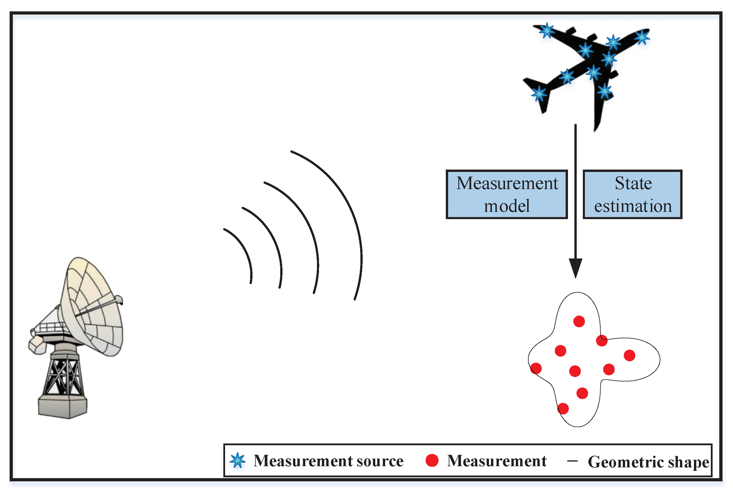
The extension state of the extended object is described by the random hypersurface model, which has an advantage over other morphological modeling methods, in that it can use more detailed information to describe some complex shapes [
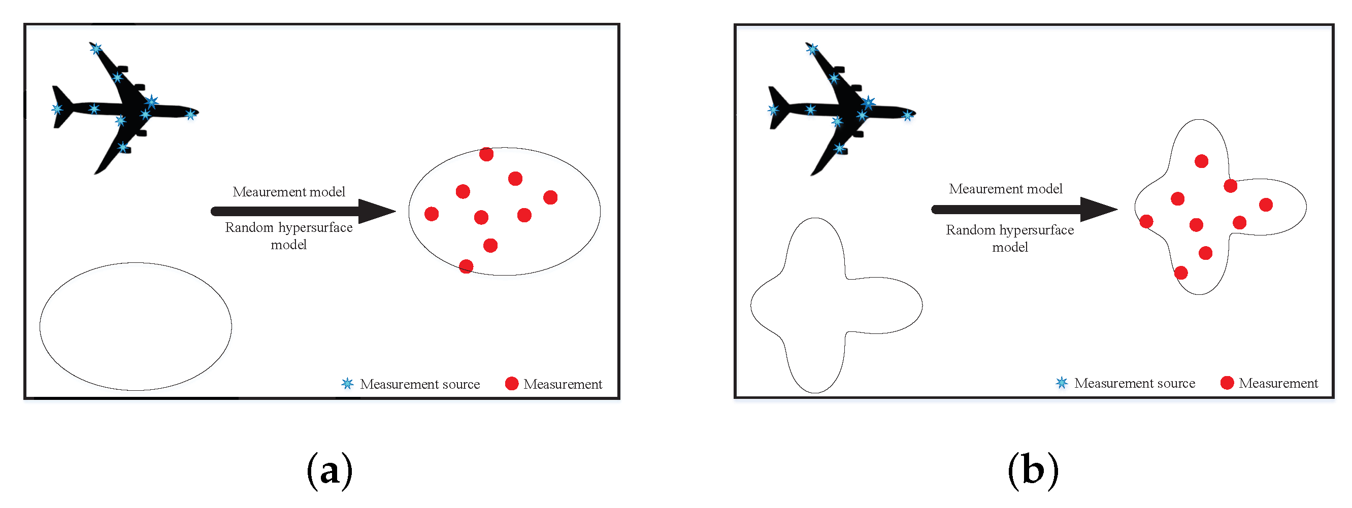
21]. For instance, the star-convex shape can more accurately approximate the true shape of the aircraft compared to other shapes (such as ellipse, see
Figure 2 below). In other words, it can model a wide range of object shapes, including irregular shapes with complex geometry. As such, more detailed features can be captured. That is why we used the random hypersurface model to model the extension state of an extended object as a star-convex shape in this paper.
2.1.1. Star-Convex Random Hypersurface Model
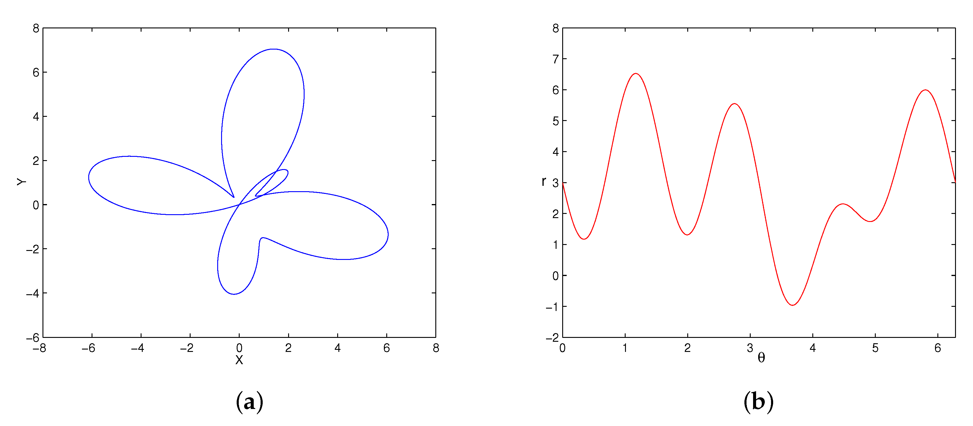
The contour of a star-convex object can be described by the radial function, and its size represents the distance between each contour point and center point of the object. As illustrated in
Figure 3,
represents the angle between the line from the center point
to the contour point, the X-axis,
denotes the distance, and
represents the scaling factor. The scaled object contour
can be described as follows:
The radial function is then linearized, i.e., Fourier series expansion is applied, which can be formulated as follows:
where
denotes the order of Fourier series expansion. In fact, the higher the order, the more detailed features can be captured. On the contrary, if the order is low, only rough features can be obtained, which will eventually result in the loss of information. Equation (
9) illustrates the coefficients expanded by the Fourier series, which can reflect the shape information of the extended object. Therefore, the extension parameter vector
of the object can be represented by
as follows:
In this paper, the extension parameter contains nine variables, i.e.,
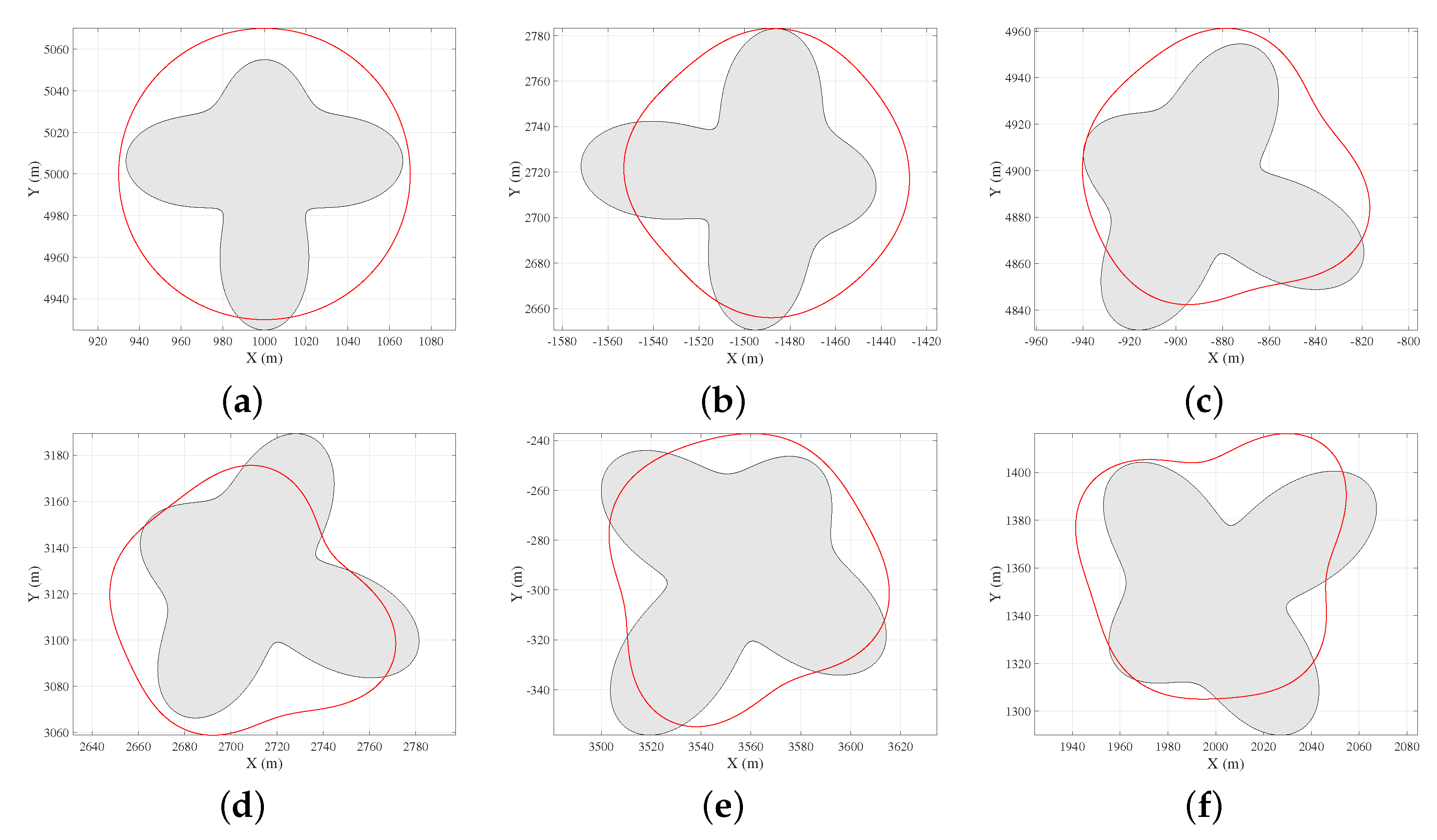
. When using the RHM to estimate the extension state, the initial shape is generally modeled as a circle, then the measurement and filtering process are used to complete the subsequent iterative process. Assuming that the object moves according to the maneuvering status in
Table 1, then a dynamic evolution process of the estimated shape can be shown in
Figure 4. Here, the black and red boundaries represent the true shape and estimated results, respectively. Initially, the shape is generally modelled as a circle, and the estimated result becomes gradually close to the true shape with the subsequent step-by-step iterative process. From
Figure 4, it can be easily noted that the estimated result gradually evolved from the initial circle to the star-convex shape.
There exists a close coupling relationship between the motion direction and orientation of the object during maneuvering. Especially in the scene of constant turning, the maneuver of the centroid and the rotation of the extended form occur simultaneously. Of course, if the object is treated as a point, the influence of maneuver on the shape does not need to be considered. Nevertheless, as for the extended object, this problem can no longer be ignored. Therefore, there is a pressing need to establish the maneuvering model of the extended object with a star-convex shape.
2.1.2. Maneuvering Modeling of Extended Object with Star-Convex Shape
The simulation test in this paper was mainly completed in the constant turning scene, so here only the evolution process of morphological variables during a turning maneuver is provided. On the one hand,
is closely related to the coefficient vector after the Fourier series expansion of the radial function. On the other hand, when the object rotates with an angle
, the radial function also shifts by the same angle [
22]. Therefore, in consideration of this property, the radial function after the rotation angle
can be calculated according to the radial function before maneuver, that is
where
defines the angle after rotation,
represents the morphological variable obtained at
, and
represents the noise in the process of morphological variable transfer. The result of Fourier expansion can be expressed as
Then, it can be further collated to the following equations.
Therefore, the variables in the extension parameter vector
are denoted as follows.
Following this, the dynamic evolution equation of morphological variables in the turning maneuver scene can be obtained as illustrated in Equation (
16), where
is the state transition matrix, which has the form expressed in Equation (
17). Taking Equations (
3) and (
17) into Equation (
1), the dynamic evolution equation of a star-convex extended object under a turning scene can be obtained.
The above model can uniformly describe the left-turning and right-turning motion of a star-convex extended object under different rotation rates. When the rotation rate is 0, the above equation degenerates into a dynamic equation of uniform linear motion [
22]. At this time, the transfer matrices of the kinematic and extension state are as follows.
However, there still exists room for improvement in the above morphological modeling process proposed in
Section 2.1.1 and
Section 2.1.2. A defect of the radial function is that there exists an implicit non-negative constraint, i.e., the distance from the center to the boundary point given an angle
must always be positive [
18]. If this important constraint is not taken into account, the estimation results will be unpredictable, which can be clearly confirmed by the example in
Figure 5. Therefore, the approximation of radial function must always be positive to ensure that it conforms to the fundamental definition of geometry, especially the star-convex shape. Nevertheless, since the radial function is a nonlinear function, only an approximate value by performing Fourier expansion during the linearization process can be obtained. It is obvious that such an operation cannot guarantee that the approximated value is always nonnegative.
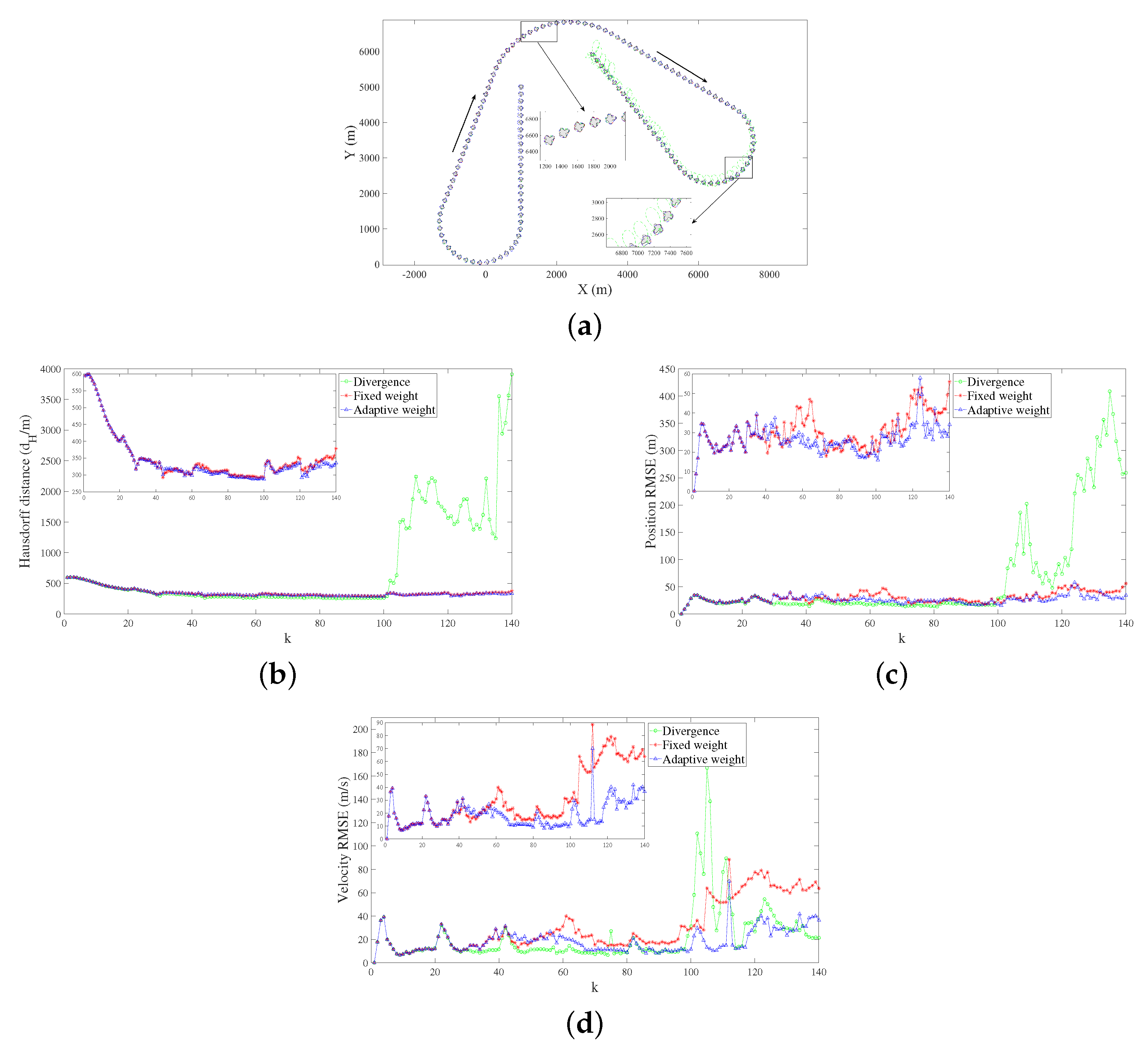
Furthermore, due to the inherent coupling relationship between shape and motion, the estimation accuracy of the kinematic state will also be significantly reduced, leading to tracking failure. As illustrated in
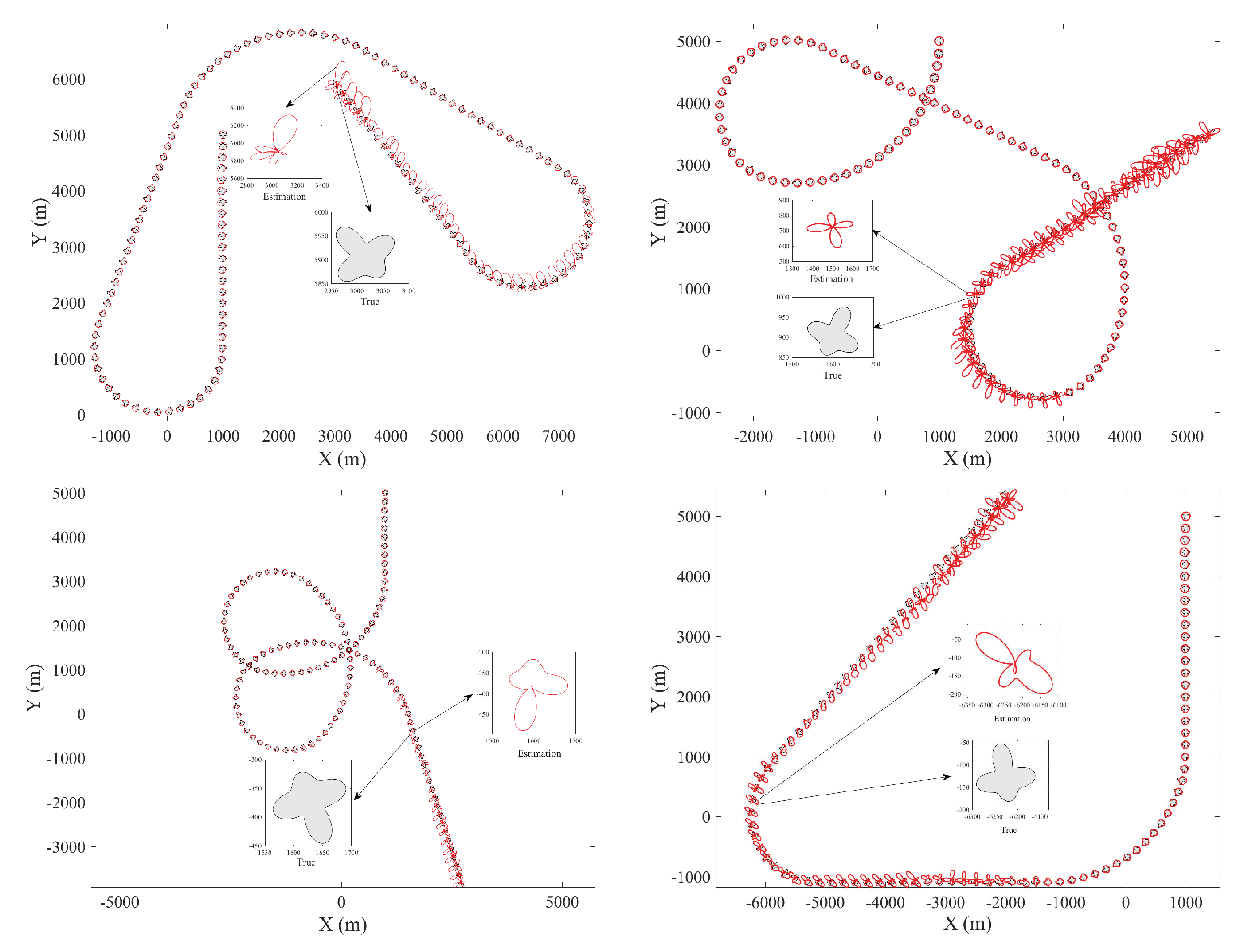
Figure 6, the estimation results of shape at some steps obviously deviated from the truth, leading to a huge estimation error. Moreover, the model itself is unable to correct this error through the subsequent iterative process. In general, it is sufficient to conclude that tracking fails due to such poor performance. Therefore, there is an urgent need to propose a novel method to avoid tracking failure once the radial function acquires a negative value.
Considering that the motion and shape of the object vary continuously between uninterrupted sampling times, i.e., there exists consistency and continuity, the parameters of the previous time must contain some information about the current time. Therefore, we can make full use of the information carried in the historical results to improve or avoid the serious consequences caused by this situation.
2.2. Proposed Approach
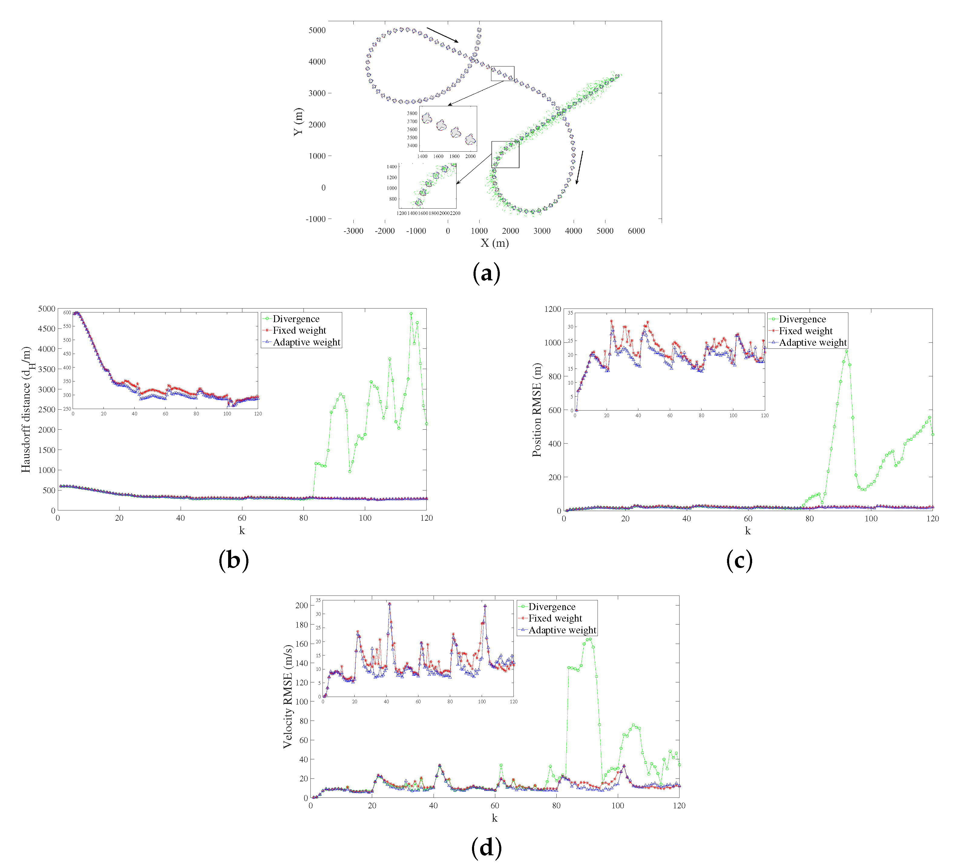
According to the previous analysis of the causes of tracking failure, the root of the problem can be found in the initialization process. Naturally, adding a novel reinitialization process to the original model to avoid tracking failure when the radial function acquires a negative value is considered in this paper. The process of reinitialization can be summarized as follows: Initially, the value of the radial function after filtering at
k is judged. If it is positive, continue with the next iteration. However, if it is negative, a novel reinitialization step needs to be executed, i.e., both the kinematic state
and extension parameter
are reinitialized. Eventually, the multi-model estimation process [
23] is performed again. The following are the specific steps of parameter reinitialization:
Assuming that denotes the shape information at the initial time, and are the kinematic state and extension parameter vectors at , respectively. Compared with the historical information of earlier steps, the state (both kinematic and extension) at is certainly closer to the current state. Therefore, the kinematic state (including position, velocity, etc.) at can be used to reinitialize . However, since the decline of estimation accuracy is fundamentally caused by shape divergence, if only the extension parameter at is utilized for the reinitialization of , it will inevitably lead to tracking failure again for the same reason. The shape at the initial time is assumed to be a circle, which belongs to a kind of convex polygon, and the radial function in the polar coordinate system must always be positive. Nevertheless, all the shape information obtained before k will be lost if only the shape at the initial time is used to reinitialize the extension parameter. This leads to a limited correction capability. Therefore, in this paper, the shape information of initial time and historical time is fused to reinitialize the extension parameter.
Since the extension parameters of the first
d steps carry the historical information of the shape, weighting of the extension parameters at the initial step and the first
d steps is considered to obtain
.
denotes the extension parameter after reinitialization, and the size of
d is determined by traversing the value of
d in this paper. Taking the second one in
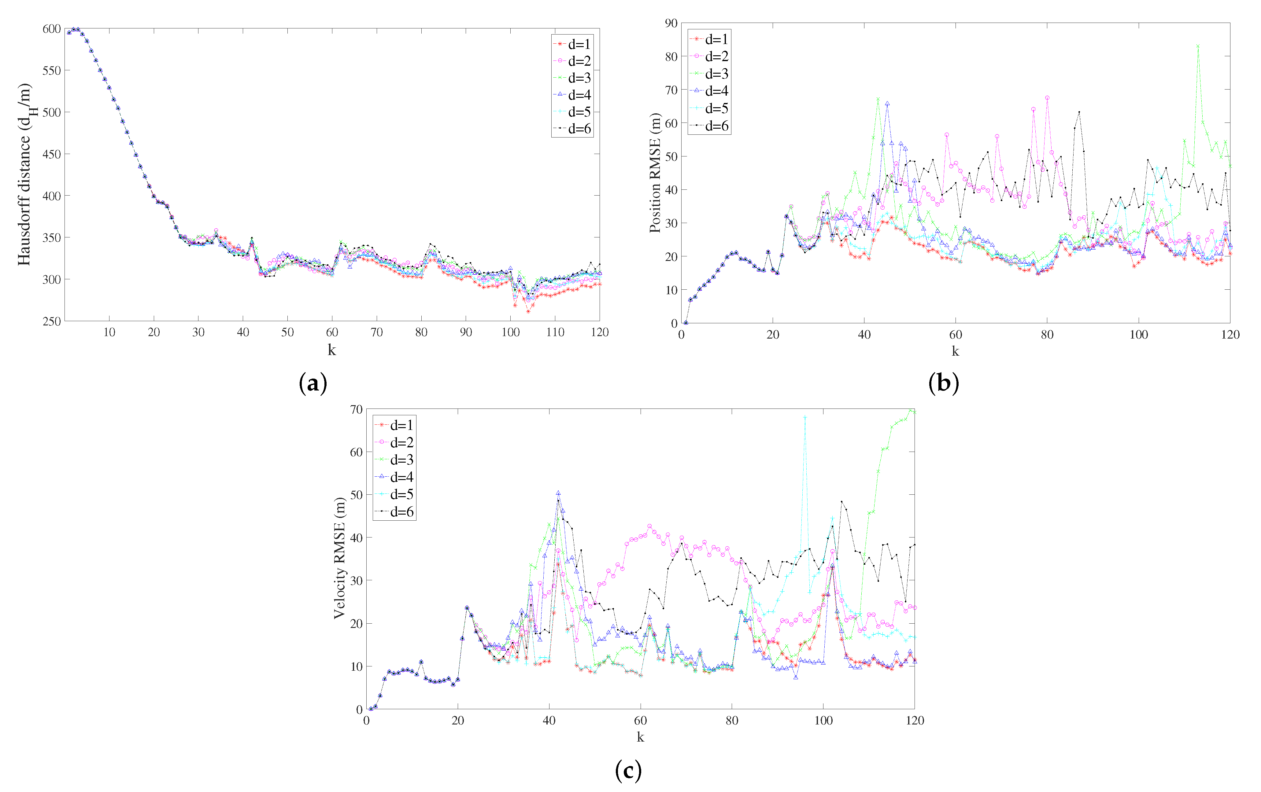
Figure 6 as the maneuvering scenario, simulation tests were conducted for different
d values from 1 to 6. Under each hypothesis, a total of 100 simulation tests were carried out.
Figure 7 and
Table 2 depict the correction ability corresponding to different
d, where Hausdorff distance [
24] and root-mean-square error (RMSE) are used to evaluate the shape and motion correction ability of different
d, respectively. The smaller the value, the better the correction capability.
As shown in
Figure 7 and
Table 2, a conclusion can be easily drawn in that the performance is the best for
. This suggests that a better correction ability can be achieved only by using the shape information at
and the initial time. This is primarily because the state of the object is continuously changing, so the shape at
(i.e.,
) actually carries the historical information of an earlier time. If
(i.e., all the information of the previous
d steps are weighted), and by reusing some historical information, the operation will not improve the correction ability but increase the computational burden. Therefore, we decided to weight
and
to obtain the extension parameter
after reinitialization.
Meanwhile, the determination of weight here is still a crucial yet difficult problem. If each weight distribution coefficient is artificially specified, a certain degree of subjective randomness is inevitably introduced. Moreover, the authority and reliability of each distribution cannot be guaranteed owing to the lack of experience. In general, the differences between the weighted extension parameter vector
and the two before combination are expected to be small. As a result, some fuzzy decision-making problems typically employ objective methods to establish a planning model for the determination of attribute weights [
25,
26]. For instance, when using the combined weighting method to evaluate the system performance, the principle of minimum relative entropy is skillfully applied to determine the distribution coefficients of subjective and objective weights [
27].
The difference between two random distributions is measured asymmetrically using relative entropy, also known as Kullback–Leibler divergence [
28]. Assuming that
and
are two probability distributions for a random variable
x, the relative entropy in the case of discrete and continuous random variables can be defined as follows, respectively [
29].
If the two probability distributions are the same, their relative entropy is zero. When the difference between the two probability distributions increases, their relative entropy will also increase. The following is an equation used to calculate weight with the principle of minimum relative entropy:
where
N indicates the number of variables in the extension parameter vector.
and
are the extension parameters at the initial time and
,
p and
q denote their weight distribution coefficients, respectively.
However, the logarithmic function’s argument must be positive, i.e., the corresponding weighted variables in
and
must have the same sign, which obviously cannot be satisfied here. Therefore, the principle of minimum relative entropy is ineffective in determining the weight distribution coefficient in this paper. It is a blessing that it can be roughly replaced by another scale criterion for measuring vector difference. Cosine distance, also known as cosine similarity, can be used to evaluate the similarity of two vectors by calculating the cosine value of the angle between them [
30]. Additionally, the difference is proportional to the cosine distance. As a result, the minimum cosine distance can be used in this paper to construct the mathematical model and calculate a more reasonable weight distribution coefficient [
31]. The process can be formulated as follows:
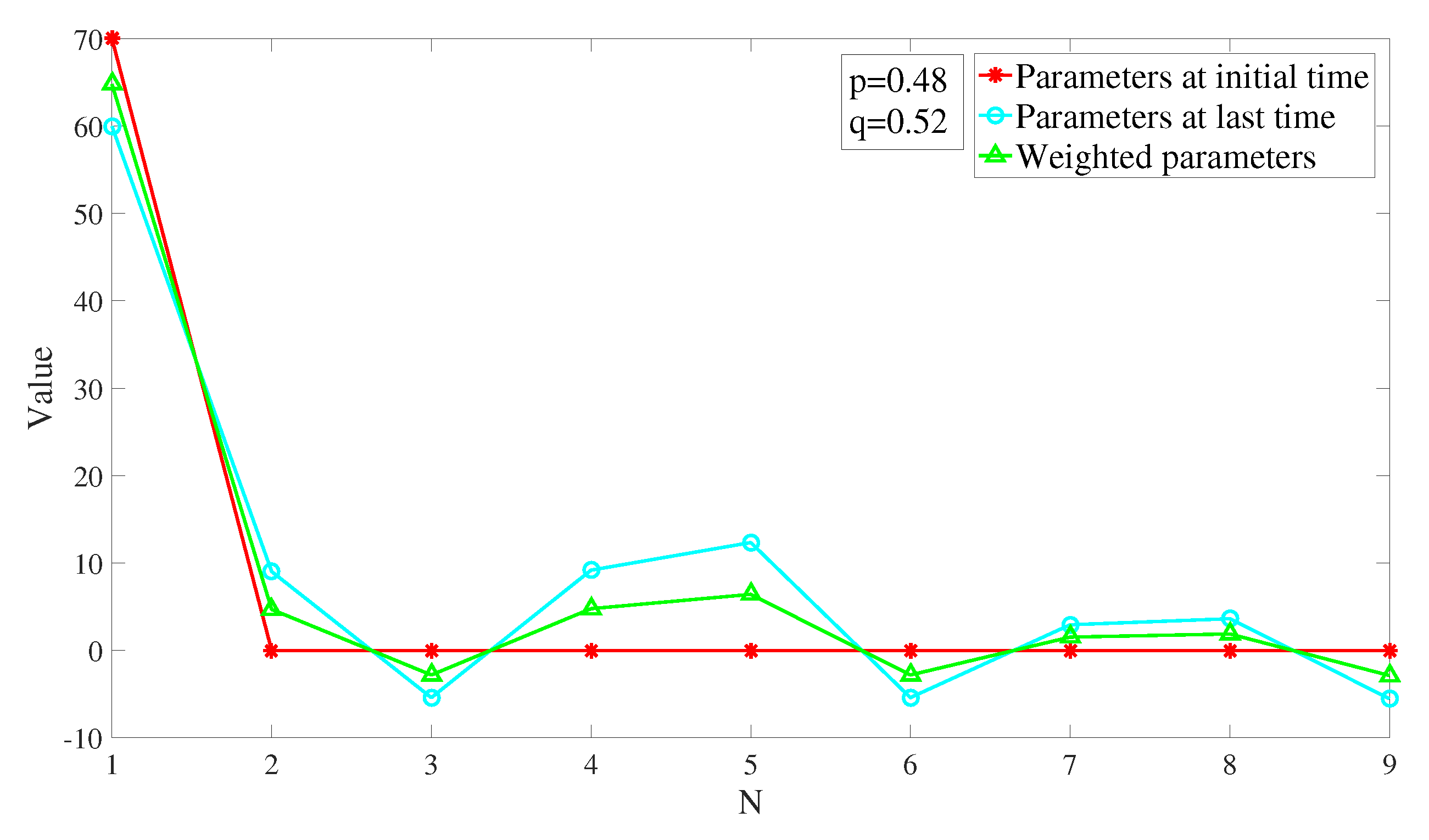
Figure 8 illustrates an example of obtaining adaptive weights
p and
q by using the minimum cosine distance in one optimization process, where the x-axis represents the number of variables included in the extension parameter vector, and the y-axis represents the values corresponding to each variable. Each time the reinitialization step is performed, the dynamic adaptive
p and
q values will be obtained according to the principle of minimum cosine distance, so as to make the weight distribution more reasonable.
Table 3 lists the complete calculation process of the modified star-convex random hypersurface model proposed above.
