Abstract
When the transmitter is in motion, the airborne passive bistatic radar (PBR) has a complex clutter geometry and lacks independent and identically distributed training samples in clutter estimation and suppression. In order to solve these problems, this paper proposes a space–time adaptive processing (STAP) algorithm based on root off-grid sparse Bayesian learning. The proposed algorithm first models the space–time base of the dictionary as an adjustable state. Then, the positions of those dynamic bases are optimized by iterating a maximum expectation algorithm. In this way, the off-grid error in clutter estimation can be eliminated even when the modeling grid is wide. To further improve the accuracy of clutter estimation, the proposed algorithm eliminates the error caused by samples with singular values in the root off-grid sparse Bayes learning by artificially adding pseudorandom noise and using hypothesis testing. The simulation results show that the proposed algorithm achieves better performance than the existing algorithms.
1. Introduction
The passive bistatic radar (PBR) [1,2,3] is a novel sensing technology. It does not actively transmit the electromagnetic waves but uses a non-cooperative opportunistic radiation source [4,5,6] (FM radio station, analog TV station, digital TV station, mobile 4G/5G base station, Wi-Fi station, satellite, etc.) as a transmitter to implement the target detection [4,6], imaging [7,8], and tracking tasks [9]. Due to the significant advantages of PBRs over traditional active radars, such as the stealth characteristics, strong anti-interception ability, and low maintenance cost, researchers have carried out a large amount of theoretical research and actual measurement experiments on PBR in recent decades. With the development of hardware techniques, the airborne PBR [10,11,12], placed on a high-altitude platform, has added attracted an increasing amount of attention. For example, the increased sensing height of the airborne PBR can help to overcome the influence of Earth curvature and increase the effective sensing range. Due to the mobility of the platform, the airborne PBR enables a flexible deployment. However, the airborne PBR still faces many challenges in practical application. For example, the high sidelobe is caused by the civil signal with continuous wave (CM) beams, the contaminated reference signal, and the strong clutter in the near area. Some researchers have proposed solutions to these problems [13,14,15,16]. Another challenge faced by the airborne PBR is to deal with the clutter spread problem caused by the movement of the receiving platform [12].
Due to the movement of the platform, the Doppler frequency of the clutter in the echo signal is no longer zero. Instead, the clutter spreads in the entire frequency domain due to the coupling relationship between the time frequency and space frequency. Therefore, the clutter suppression algorithm proposed for the traditional ground-based PBRs [17] is no longer applicable to airborne PBRs. The space–time adaptive processing (STAP) algorithm can effectively suppress the clutter of the airborne radar by using the space–time two-dimensional correlation method [18,19,20]. This approach considers the problem of clutter Doppler broadening caused by the movement of the receiving platform. However, in addition to this problem, the influences of the dual-base configuration and the motion state of the transmitting source on the clutter should also be considered.
When the non-cooperative transmitting source is fixed, its side-looking observation mode is equivalent to the clutter model of the traditional active side-looking radar, and this indicates that the coupling relationship of the space–time clutter is presented as a diagonal shape distribution in the space–time frequency spectrum plane. When the transmitting source is in motion, the relative motion relationship between the transmitting source and the receiving platform can be complex. The coupling relationship of the spatial–temporal clutter changes correspondingly. In the spatial–temporal frequency spectrum, it is no longer a diagonal shape distribution but a complex geometric relationship. The air-to-air bistatic configuration increases the clutter complexity. Additionally, this configuration further increases the difficulty of clutter estimation because it reduces the number of independent and identically distributed (IID) training samples in clutter estimation.
In order to effectively estimate the clutter of the airborne PBR with a limited number of IID samples, three existing algorithms are available: Reduced-dimensional STAP (RD–STAP) [21,22], reduced-rank STAP (RR–STAP) [23,24], and sparse recovery STAP (SR–STAP) [25,26,27,28]. Although the RD–STAP and RR–STAP algorithms can reduce the number of training samples, they still need a large number of IID training samples. Therefore, these algorithms are not applicable for airborne PBRs.
Based on the sparsity of the airborne PBR clutter in the space–time plane, the SR-STAP algorithm can estimate the clutter using a small number of IID training samples by setting an over-complete dictionary basis of spatial–temporal steering vectors. There are extensive research studies on the SR–STAP algorithm [25,26,27,28]. However, these studies assume a side-view monitoring mode of the airborne active radar and are hence not applicable to the clutter suppression of the airborne PBR. The space–time sparse approach has an off-grid effect due to the geometric complexity of the airborne PBR clutter, that is, the location of the space–time clutter is mismatched with the uniformly divided space–time guide vector grid. It is necessary to consider the estimation and suppression of the space–time off-grid clutter.
There are three methods to solve the off-grid problem in sparse estimation, i.e., the increased dictionary base density, the local refinement [29,30,31], and the atomic norm minimization [31]. Increasing the dictionary base density can increase the correlation between different dictionary bases and reduce the accuracy of sparse recovery. The local refinement method needs to be split at each off-grid location, requiring a large amount of computation. Additionally, the method cannot be effectively restored under the rough model condition. The atomic norm minimization method is sensitive to the low-rank characteristics and has high computational complexity due to the interior point approach. Since the calculation of the PBR signal data is huge, both the local refinement method and the atomic norm minimization method cannot effectively estimate the space–time clutter in the airborne PBR.
In order to solve the problem of space–time clutter estimation and suppression for the airborne PBR, a space–time adaptive algorithm based on root off-grid sparse Bayes learning is proposed. This algorithm is mainly derived from the concepts of SBL [32,33,34] and RSBL [35,36], and estimates the off-grid space–time clutter. The proposed algorithm first establishes a space–time steering vector dictionary with a wide grid, then sets the position of the space–time clutter as a variable parameter, and finally uses the maximum expectation (EM) algorithm to iteratively optimize the position to estimate the position and amplitude of the space–time clutter. Therefore, this algorithm can estimate and suppress the off-grid space–time clutter of the airborne PBR with few IID training samples and a small amount of computation. To further improve the accuracy of clutter estimation, the proposed algorithm has been further optimized based on RSBL, named pseudorandom root off-grid sparse Bayes STAP (PROGSBL–STAP). The PROGSBL–STAP algorithm adds pseudorandom noise to original samples [37,38,39], then performs resampling and re-estimation, and finally, uses the hypothesis-testing criteria to select effective training samples. The PROGSBL–STAP algorithm can eliminate the error caused by samples with singular values. Simulation experiments show that the PROGSBL–STAP algorithm performs better than existing algorithms for the off-grid space–time clutter estimation of airborne PRBs.
The rest of this paper is arranged as follows: Section 2 introduces the signal model, clutter model and presents the PROGSBL–STAP algorithm. In Section 3, simulation experiments are used to verify the effectiveness of the proposed algorithm. Section 4 presents discussions of the experimental results and Section 5 concludes the paper.
The definitions of some necessary notations are provided in Table 1.

Table 1.
Some important notations.
2. Method
2.1. Signal Model of PBR System and Traditional STAP
In this subsection, we present the signal model and clutter model of the airborne PBR and introduce the traditional STAP algorithm for clutter estimation and suppression.
2.1.1. Signal Model of PBR System
The geometric structure of the airborne PBR system considered in this paper is shown in Figure 1, in which a low-orbit satellite is used as the signal emitter. The PBR flies at altitude H and speed , the reference sensor of the radar is pointed at the moving emitter, a uniform linear array (ULA) composed of sensors is used as a set of surveillance sensors to point to the surveillance area, the distance between the array elements is , and the speed of the emission source is .
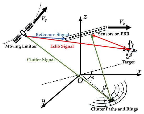
Figure 1.
The geometric structure of the airborne PBR system.
The reference signal received by the reference sensor can be expressed as follows:
where denotes the number of equivalent pulses, denotes the pulse repetition interval, denotes the complex amplitude of the reference signal, denotes the Doppler frequency of the reference direct wave signal, represents the complex envelope of the reference signal, and denotes the noise in the reference sensor.
The echo signal from the -th reflection point received by the -th surveillance sensor can be expressed as follows:
where denotes the complex amplitude of the echo signal from the corresponding reflection, denotes the time delay, and and denote the temporal and spatial frequency, respectively, denotes the noise of the -th surveillance sensor.
The cross-correlation result between the reference signal and the echo signal can be expressed as follows:
where , . denotes the noise component.
Taking the fast Fourier transform of obtains:
2.1.2. Traditional STAP
It can be observed in Figure 1 and Equation (4) that, in the same distance unit, the received clutter can be equivalent to an equidistant clutter ring, so the clutter ring signal of the -th distance unit can be expressed as follows:
where denotes the number of clutter points in an equidistant ring, and denote the spatial and temporal steering vectors, respectively.
According to the STAP algorithm, the space–time clutter cancellation weight factor of the -th distance unit to be detected can be expressed as follows:
where .
Since in Equation (6) cannot be obtained directly, the method of averaging the distance units to be detected is generally adopted in the traditional space–time adaptive algorithm, that is:
where denotes the number of IID training samples. Generally, when the airborne PBR works in a complex environment, cannot reach twice the space–time degrees of freedom , which is required by the RMB criterion. Therefore, the traditional STAP algorithm cannot effectively complete the clutter estimation and suppression.
2.2. STAP Algorithm Based on Root Sparse Bayes Learning
This subsection presents the sparse recovery model of space–time clutter and the traditional sparse STAP algorithm, and proposes the modified algorithm named PROGSBL–STAP algorithm.
2.2.1. Sparse Recovery Model of Space–Time Clutter
In the traditional SR–STAP algorithm [25,26,27,28], the spatial–temporal clutter is usually estimated by constructing an overcomplete sparse recovery dictionary, and the dictionary is obtained by discretizing the angle-Doppler plane.
The space–time plane is uniformly discretized into grid points along the spatial angular frequency axis and the Doppler frequency axis, where , , parameters and are the corresponding meshing coefficients and . The discretized spatial frequency and Doppler frequency interval can be expressed as and . The network points formed after discretization correspond to the steering vectors in the space–time dictionary. Assuming that some clutter points are located at the grid points, the snapshot in Equation (5) can be expressed as:
where denotes the observation snapshot, denotes the constructed sparse recovery dictionary (its dimension is ), denotes the vector of sparse recovery complex coefficients, denotes the noise and can be expressed in detail as follows:
Equation (8) represents the single snapshot model. The multi-snap format of Equation (8) can be expressed as follows:
where , and .
The space–time clutter spectrum can be estimated by solving in Equation (8) or in Equation (10) through conventional sparse recovery methods.
2.2.2. STAP Based on Root Off-Grid Sparse Bayesian Learning
Aiming to solve the off-grid problem of sparse vector for dictionary , this subsection proposes a root off-grid sparse Bayesian learning algorithm to effectively estimate the clutter of the airborne PBR.
It is assumed that the noise in the airborne PBR is a complex Gaussian random variable [32,33], its mean is and the variance is . Regarding the training data in the distance unit, the conditional probability density function of the observation vector can be expressed as follows:
where , , denotes space–time dictionary bases with adjustable bases, and and denote the noise variance. Commonly, can be assumed to obey a Gamma distribution hierarchical prior:
where denotes generalized hyperparameters.
Suppose that the prior probability of the sparse vector representing the spatial–temporal clutter follows a Gaussian distribution with a zero mean value, the prior probability density function is as follows:
where denotes that the inverse of the variance of and are non-negative parameters. In the process of sparse Bayesian learning, the correlation vector machine decision mechanism determines that most elements of tend to infinity, that is, when , the variance of tends to zero.
The prior probability density function of can be obtained as follows:
where and .
Since cannot be computed explicitly, Bayesian inference via EM algorithm is considered. In the E step of the EM algorithm, a lower bound is constructed on the prior function, and this lower bound is optimized in the M step. The EM algorithm in SBL [29] can be expressed as follows:
E step:
where
To achieve the convergence of and , the well-known sparse Bayesian equivalent lower bound formula can be obtained as follows:
M step:
By maximizing , the updated values of and can be obtained as follows:
where .
By ignoring the irrelevant parameters, the updating of can be solved by maximizing the following equation:
In order to refine the treatment of each or its exponential form, , take the partial derivative of the equation with respect to , and set the partial derivative to zero, then obtain Equation (22):
where , and denote the -th column, the -th element, and the -th element of , respectively. It can be obtained from Equation (22):
Further simplifying Equation (22), it can be obtained:
Selecting the root closest to the identity element, the estimated angle of the refined mesh is as follows:
2.2.3. Pseudo Resampling Root Off-Grid Sparse Bayesian Learning STAP Algorithm
Compared with the traditional STAP algorithm, the root off-grid sparse Bayesian learning STAP algorithm has better clutter estimation performance than the traditional STAP algorithm in the case of a small number of IID training samples. Additionally, the proposed method can still maintain excellent performance under the condition of a wide dictionary grid and low computational cost. However, this method may still cause clutter outliers due to the mismatch of the base grid, and the existence of outliers will cause large clutter estimation errors. In order to reduce these errors caused by outliers, based on the root-based sparse Bayesian learning STAP algorithm, this paper further proposes a pseudo resampling root-based sparse Bayesian learning STAP algorithm.
In the proposed algorithm, appropriate noise [37,38,39] is artificially added to sample the values with large errors multiple times for some estimated values with large estimation errors in the clutter results obtained using the root off-grid sparse Bayesian learning STAP algorithm. When obtaining the new sample values after multiple estimations, the estimated values with smaller errors are screened out through the generated sector range, and the mean value of the new estimated values is calculated again, which is the final clutter estimation result of this algorithm.
The essence of this algorithm is to add the artificial noise to the received samples, which can be expressed as follows:
where denotes the artificial noise.
After adding the artificial noise, the clutter estimation result can be obtained from the dictionary basis matrix and sparse vector in the initially received sample through the iterative convergence of the root-based sparse Bayesian STAP algorithm. For this series of estimated values, it must be determined whether the estimated values are within the error range. If the estimated values are all within the error range, the resample processing of the values is not necessary; otherwise, the estimated data with larger errors need to be resampled, which requires a practical test criterion to determine the estimated value. For this requirement, assume the following test criteria:
When the hypothesis-testing criterion detects that an estimated value is distributed within , it is regarded as a normal estimate. If the estimated value fails to pass criterion , the original clutter estimate can be disturbed by generating pseudonoise to obtain the group of estimated values; only if group can pass the criterion , then the estimated values of group can be averaged to meet the conditions, so the following results can be obtained:
In Equation (28), when , no perturbation resampling of the original data is required. When , the estimated value is calculated using Equation (28). Set as the pre-obtained space–time frequency screening area:
where represents the space–time frequency corresponding to the left and right critical points obtained by the peak drop 3 dB of the -th estimated value, represents the highest peak in space–time frequency corresponding to the -th estimate value, . If the effective distance between the tested trough and the trough does not exceed 3dB, then the space–time frequency value on the curve corresponding to the position of the two troughs is determined as . The estimated value obtained via the following definition for each resampling of IID samples is as follows:
where is the estimated value of the space–time clutter point obtained by the -th resampling, and the times of sampling for the clutter to be estimated are as follows:
The space–time frequency estimated by the proposed algorithm in this paper is divided into two sets, one of which falls within , and the other falls outside of . The final clutter estimation result only uses the space–time frequency points that fall into , the values outside are discarded. This algorithm improves the accuracy of clutter estimation. This algorithm, based on the distributed reliability detection strategy, can effectively improve the accuracy of clutter estimation. By analyzing a large number of experimental results, the output of clutter estimation tends to converge with the resampling time of 30. Therefore, in order to ensure that the generality is not lost, this paper adopts the number .
2.3. Algorithm Summary
The steps of the algorithm proposed in Section 3.2 and Section 3.3 are summarized in Algorithm 1.
| Algorithm 1. ROG-SBL STAP Algorithm |
| (1) Set the independent and identically distributed training samples of the airborne PRB as the observation vector in Equation (10). |
| (2) Initialization: the variable , ; hyperparameters , ; the algorithm iteration convergence threshold ; and the maximum number of iterations . |
| (3) When the number of iterations and , continue steps (4), (5), and (6). |
| (4) Update and from Equations (16) and (17). |
| (5) Update and from Equations (19) and (20). |
| (6) Update from Equation (26), then go back to step (3). |
| (7) Add artificial noise according to Equation (27). |
| (8) If , is the final estimate value. |
| (9) If , re-estimate according to Equations (30) and (31). |
| (10) Estimate based on the obtained , , , and according to Equations (13) and (14). |
| (11) Estimate of the airborne PBR based on and in Equation (6), end. |
3. Results
3.1. Spatial–Temporal Clutter Spectrum
This experiment evaluates the performance of the proposed algorithm by comparing the space–time clutter spectra obtained using the proposed algorithm with three other existing algorithms (traditional STAP algorithm [17], traditional SR–STAP algorithm [22,23,24,25], and BCS–STAP algorithm [30]). The key parameters used in the simulation are shown in Table 2, in which the non-cooperative transmitting source and transmitting signal adopt parameters close to GPS, and this experiment and subsequent experiments were carried out using MATLAB2021 software. In the experiment, in order to reflect the off-grid computing performance advantage of this algorithm, the space–time dictionary of the traditional SR–STAP, BCS–STAP, and the PROGSBL–STAP algorithms in this paper is divided into the same grid grids. Furthermore, in order to reflect the adaptability of the algorithm to the bistatic PBR configuration, four typical different relative motion relationships between the transmitter and the receiver are selected for verification in this paper. Figure 2 shows the experimental results of this section.
Table 2.
Simulation parameters.
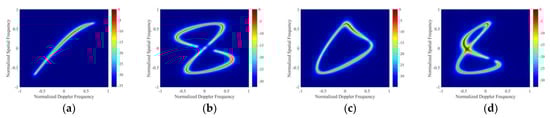
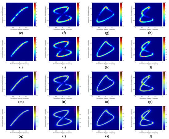
Figure 2.
Spatial–temporal clutter spectra of: (a) OPT in relationship 1, (b) OPT in relationship 2, (c) OPT in relationship 3, (d) OPT in relationship 4, (e) Traditional STAP algorithm used in relationship 1, (f) Traditional STAP algorithm used in relationship 2, (g) Traditional STAP algorithm used in relationship 3, (h) Traditional STAP algorithm used in relationship 4, (i) Traditional SR–STAP algorithm used in relationship 1, (j) Traditional SR–STAP algorithm used in relationship 2, (k) Traditional SR–STAP algorithm used in relationship 3, (l) Traditional SR–STAP algorithm used in relationship 4, (m) BCS–STAP algorithm used in relationship 1, (n) BCS–STAP algorithm used in relationship 2, (o) BCS–STAP algorithm used in relationship 3, (p) BCS–STAP algorithm used in relationship 4, (q) PROGSBL–STAP algorithm used in relationship 1, (r) PROGSBL–STAP algorithm used in relationship 2, (s) PROGSBL–STAP algorithm used in relationship 3, (t) PROGSBL–STAP algorithm used in relationship 4.
Figure 2a–d shows the optimal (OPT) clutter spectrum when IID samples are sufficient as a comparison of the four algorithms. From Figure 2e–h, it can be seen that the traditional STAP algorithm cannot effectively complete the spatial–temporal clutter estimation when the IID training samples are insufficient. From Figure 2i–l, it can be seen that the traditional SR–STAP can take advantage of the sparse recovery algorithm to show better clutter estimation performance than the traditional STAP under the condition of insufficient IID samples, but the estimated clutter spectrum is relatively incomplete, and there is a serious off-grid situation. From Figure 2m–p, it can be seen that compared with the traditional SR–STAP algorithm, the BCS–STAP algorithm shows better clutter estimation performance and can slightly correct the off-grid phenomenon. Finally, as shown in Figure 2q–t, the PROGSBL–STAP algorithm proposed in this paper can complete high-quality spatial–temporal clutter spectrum estimation, and can better correct the off-grid problem. The experimental results are close to the OPT in Figure 2a–d.
3.2. Improvement Factor of Signal-to-Noise Ratio
In order to further quantitatively analyze the clutter suppression performance of the proposed algorithm, this experiment simulates the relationship between the signal-to-noise ratio improvement factor (IF) and the normalized Doppler frequency of the distance unit to be detected. The IF can be obtained using Equation (32), which is represented as follows:
where can be derived from Equation (6).
Figure 3a–d shows the SINR loss curves of relationships 1, 2, 3, and 4, respectively, and the results are the average of 300 Monte Carlo experiments. It can be seen that in relationships 1, 2, 3, and 4, all four algorithms can form a zero limit where space–time clutter exists, and the clutter suppression performance is in order from low to high: Traditional STAP, traditional SR–STAP, BCS–STAP, and PROGSBL–STAP. The proposed algorithm (PROGSBL–STAP) has better clutter suppression performance than the existing three algorithms, and the results of the PROGSBL–STAP algorithm are almost close to OPT.
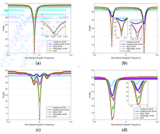
Figure 3.
Comparison of improvement factor (IF) with different algorithms in: (a) relationship 1, (b) relationship 2, (c) relationship 3 and (d) relationship 4.
As a further quantitative analysis, in order to compare the clutter suppression performance of each algorithm with different IID training samples, this experiment calculates the relationship between the average IF value(dB) of each algorithm with the reduced number of IID training samples at the zero spatial-Doppler. Figure 4a–d shows the IF curves of relationships 1, 2, 3, and 4, respectively, and the results are the average of 300 Monte Carlo experiments. It can be seen that with the reduction of the number of IID samples, the clutter suppression performance of each algorithm is ranked from high to low as: PROGSBL–STAP, BCS–STAP, traditional SR–STAP, and traditional STAP. Especially when the number of training samples is from 10 to 3, the clutter performance of the proposed PROGSBL–STAP algorithm can still maintain an advantage over the existing algorithm, and the performance is close to OPT.
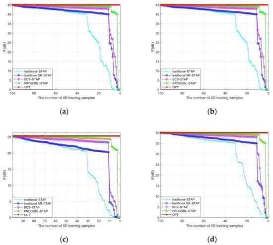
Figure 4.
IF versus the number of IID training samples with different algorithms in: (a) Relationship 1, (b) relationship 2, (c) relationship 3, and (d) relationship 4.
3.3. Performance with Dictionary Grid Width
Based on the experiment in Section 3.1, this experiment takes relationship 2 as an example and compares the spatial–temporal clutter spectrum of the PROGSBL-STAP algorithm with the traditional SR-STAP algorithm and BCS-STAP algorithm by setting different spatial–temporal dictionary grids, so as to further verify the off-grid performance advantages of the PROGSBL-STAP algorithm.
Figure 5a,d,g shows the processing results of using the traditional SR–STAP algorithm 1 under grid , grid , and grid , respectively. Figure 5b,e,h shows the processing results of using the traditional SR–STAP algorithm 1 under grid a , grid , and grid , respectively. Figure 5c,f,i presents the processing results of using the traditional SR–STAP algorithm 1 under grid , grid , and grid , respectively.
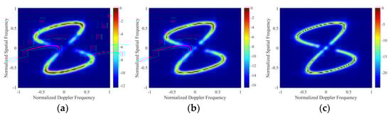
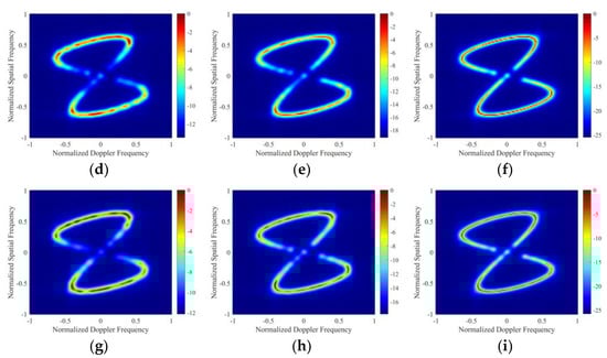
Figure 5.
Spatial–temporal clutter spectra in relationship 1: (a) Traditional SR–STAP (grid ), (b) BCS–STAP (grid ), (c) PROGSBL–STAP (grid ), (d) traditional SR–STAP (grid ), (e) BCS–STAP (grid ), (f) OROGSBL–STAP (grid ), (g) traditional STAP (grid ), (h) BCS–STAP (grid ), (i) PROGSBL–STAP (grid ).
From Figure 5a–i, it can be seen that the proposed PROGSBL–STAP algorithm has better spatial–temporal clutter estimation performance and better off-grid performance than the existing two algorithms when the dictionary grid is wide.
In order to further quantitatively analyze the off-grid performance of the PROGSBL–STAP, this experiment compared the three algorithms with the Cramer–Rao Bound (CRB). The performance improvement of the proposed algorithm was verified by calculating the relation between the space time estimated root mean square error (RMSE) and the grid interval. The results calculated at SNR 10 dB and 25 dB were the average of 300 Monte Carlo experiments.
From Figure 6a,b, it can be seen that the PROGSBL–STAP algorithm is superior to the traditional SR–STAP algorithm and BCS–STAP algorithm, especially when the mesh spacing is large. The reason for this is that when the mesh is thick, the traditional SR–STAP algorithm and BCS–STAP algorithm will lead to high modeling error usage, while the PROGSBL–STAP algorithm can correctly handle the modeling error mesh as adjustable parameters using the rough sampling position.
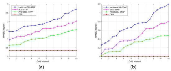
Figure 6.
RMSE of spatial–temporal clutter estimates versus grid interval at (a) SNR 10dB and (b) SNR 25dB.
3.4. Improved Performance with Singular Value
In this experiment, based on the 4 flight relationships in Section 3.1, singular values are added to the original spatial–temporal clutter samples. The advantages of the proposed PROGSBL algorithm are demonstrated by comparing the experimental results of whether to use pseudorandom noise optimization, that is, comparing the spatial–temporal clutter spectrum in PROGSBL–STAP (before eliminating singular samples) and PROGSBL–STAP (after eliminating singular samples).
From Figure 7a–h, it can be seen that, in the space–time clutter spectrum of relationships 1, 2, 3, and 4, the estimation performance of the PROGSBL–STAP (before eliminating singular samples) is affected by singular values in Figure 7a,c,e,f, while the PROGSBL–STAP (after eliminating singular samples) can better achieve accurate clutter spectrum estimation when there are singular values in the clutter training sample in Figure 7b,d,f,h.
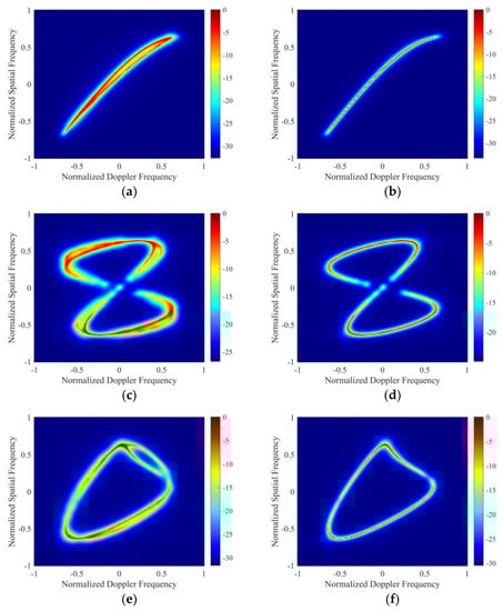
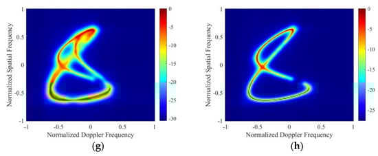
Figure 7.
Spatial–temporal clutter spectra (a) in relationship 1: PROGSBL–STAP (before eliminating singular samples), (b) PROGSBL–STAP (after eliminating singular samples), (c) in relationship 2: PROGSBL–STAP (before eliminating singular samples), (d) in relationship 2: PROGSBL–STAP (after eliminating singular samples), (e) in relationship 3: PROGSBL–STAP (before eliminating singular samples), (f) in relationship 3: PROGSBL–STAP (after eliminating singular samples), (g) in relationship 4: PROGSBL–STAP (before eliminating singular samples), (h) PROGSBL–STAP (after eliminating singular samples).
In order to further quantitatively analyze the singular samples elimination performance of the PROGSBL–STAP, this experiment simulates the relationship between the signal-to-noise ratio IF and the normalized Doppler frequency of the distance unit to be detected. The IF can be obtained using Equation (32), and the results are the average of 300 Monte Carlo experiments.
From Figure 8a–d, it can be seen that in the flight relationship 1–4, affected by the singular value samples, the IF curves all have zero limits at the positions where the singular values exist. These zero limits that should not exist will eliminate the target at the corresponding position while suppressing the clutter. After the singular sample elimination of the PROGSBLSTAP algorithm, the IF curve shows normal performance and can perform correct clutter suppression.
Figure 8.
IF comparison before and after singular sample elimination in: (a) Relationship 1, (b) relationship 2, (c) relationship 3, and (d) relationship 4.
4. Discussion
The above experiments have obtained a large number of qualitative and quantitative analysis results. These experimental results show that: (1) The proposed PROGSBL-STAP algorithm has obvious clutter estimation and suppression performance advantages over the existing algorithms in various complex geometric configurations of the airborne PBR (Figure 2 and Figure 3), (2) with the reduction of the number of IID training samples, the proposed PROGSBL-STAP algorithm has more advantages than existing algorithms, especially under the condition of very few training samples (Figure 4), (3) the proposed PROGSBL-STAP algorithm has better off-grid clutter estimation performance than existing algorithms (Figure 5 and Figure 6), (4) when there are singular values in the training samples, the proposed PROGSBL-STAP algorithm can eliminate the influence of singular values and maintain excellent clutter suppression performance (Figure 7 and Figure 8).
5. Conclusions
In this paper, a space–time adaptive processing algorithm based on root off-grid sparse Bayes learning is proposed when the emission source of the airborne PBR is in motion, namely, the PROGSBL–STAP algorithm. The algorithm first sets the space–time dictionary base to an adjustable state, and then uses the EM algorithm to iteratively optimize the position of the base, thereby improving the estimation performance of off-grid clutter. The simulations show that the proposed algorithm has obvious advantages over the existing algorithms when the modeling grid is wider. In addition, the ROGGSBL-STAP algorithm adds pseudorandom noise to the original sample, resamples and re-estimates, and finally selects effective training samples according to the hypothesis-testing criteria. The simulation results show that the PROGGSBL-STAP algorithm has better clutter estimation performance when singular values exist in the training samples. In summary, the proposed PROGSBL-STAP algorithm has better performance than existing algorithms in the clutter estimation and suppression of the airborne PBR in complex environments and geometric configurations.
Author Contributions
The work described in this article was collaboratively developed by all authors. J.W. (Jipeng Wang) and J.W. (Jun Wang) contributed to data processing and designed the algorithm. J.W. (Jipeng Wang) and L.Z. made contributions to data measurement and analysis. J.W. (Jipeng Wang) participated in the writing of the paper. S.G. and D.Z. revised the writing of the paper. All authors have read and agreed to the published version of the manuscript.
Funding
This research was funded by the support of Key Laboratory of Space Microwave Technology under Grant 6142411342104 and the stabilization support of National Radar Signal Processing Laboratory under Grant KGJ202102.
Data Availability Statement
No new data were created or analyzed in this study, so data sharing is not applicable.
Acknowledgments
The authors would like to thank the laboratory and university for their support.
Conflicts of Interest
The authors declare no conflict of interest.
References
- Kuschel, H.; Cristallini, D. Olsen K E. Tutorial: Passive radar tutorial. IEEE Aerosp. Electron. Syst. Mag. 2019, 34, 2–19. [Google Scholar] [CrossRef]
- Griffithsm, H.; Baker, C.J. An Introduction to Passive Radar; Artech House: Norwood, MA, USA, 2017. [Google Scholar]
- Malanowski, M. Signal Processing for Passive Bistatic Radar; Artech House: Norwood, MA, USA, 2019. [Google Scholar]
- Li, Y.; Ma, H.; Cheng, L.; Yu, D. Method for bearing estimation of target for amplitude modulation radio-based passive radar application. Electron. Lett. 2018, 54, 383–385. [Google Scholar] [CrossRef]
- Colone, F. DVB-T-Based Passive Forward Scatter Radar: Inherent Limitations and Enabling Solutions. IEEE Trans. Aerosp. Electron. Syst. 2020, 57, 1084–1104. [Google Scholar] [CrossRef]
- Sun, H.; Chia, L.G.; Razul, S.G. Through-Wall Human Sensing with WiFi Passive Radar. IEEE Trans. Aerosp. Electron. Syst. 2021, 57, 2135–2148. [Google Scholar] [CrossRef]
- Imperatore, P. SAR Imaging Distortions Induced by Topography: A Compact Analytical Formulation for Radiometric Calibration. Remote Sens. 2021, 13, 3318. [Google Scholar] [CrossRef]
- Andriyanov, N.; Andriyanov, D. Modeling and processing of SAR images. In Proceedings of the VI International Conference Information Technology and Nanotechnology, Samara, Russia, 26–29 May 2020. [Google Scholar]
- Zhu, Y.; Liang, S.; Gong, M.; Yan, J. Decomposed POMDP Optimization-Based Sensor Management for Multi-Target Tracking in Passive Multi-Sensor Systems. IEEE Sens. J. 2022, 22, 3565–3578. [Google Scholar] [CrossRef]
- Tan, D.K.P.; Lesturgie, M.; Sun, H.; Lu, Y. Space-time interference analysis and suppression for airborne passive radar using transmissions of opportunity. IET Radar Sonar Navig. 2014, 8, 142–152. [Google Scholar] [CrossRef]
- Qi, D.; Feng, B.; Feng, W.; Zhang, Z.; He, X.; Shang, C. Digital TV Signal Based Airborne Passive Radar Clutter Suppression via a Parameter-Searched Algorithm. Wirel. Pers. Commun. 2021, 120, 3189–3216. [Google Scholar] [CrossRef]
- Rosenberg, L.; Duk, V. Land Clutter Statistics from an Airborne Passive Bistatic Radar. IEEE Trans. Geosci. Remote Sens. 2021, 60, 5104009. [Google Scholar] [CrossRef]
- Deng, Y.; Wang, J. Cascaded suppression method based on joint iterative optimization for airborne passive radar. Digit. Signal Process. 2020, 100, 102686. [Google Scholar] [CrossRef]
- Sui, J.X.; Wang, J.; Zuo, L.; Gao, J. Cascaded Least Square Algorithm for Strong Clutter Removal in Airborne Passive Radar. IEEE Trans. Aerosp. Electron. Syst. 2021, 58, 679–696. [Google Scholar] [CrossRef]
- Yang, P.-C.; Lyu, X.-D.; Chai, Z.-H.; Zhang, D.; Yue, Q.; Yang, J.-M. Clutter Cancellation Along the Clutter Ridge for Airborne Passive Radar. IEEE Geosci. Remote Sens. Lett. 2017, 14, 951–955. [Google Scholar] [CrossRef]
- Guo, S.; Wang, J.; Ma, H.; Wang, J. Modified Blind Equalization Algorithm Based on Cyclostationarity for Contaminated Reference Signal in Airborne PBR. Sensors 2020, 20, 788. [Google Scholar] [CrossRef] [PubMed]
- Zuo, L.; Wang, J.; Sui, J.; Li, N. An Inter-Subband Processing Algorithm for Complex Clutter Suppression in Passive Bistatic Radar. Remote Sens. 2021, 13, 4954. [Google Scholar] [CrossRef]
- Guerci, J.R. Space-Time Adaptive Processing for Radar; Artech House: Norwood, MA, USA, 2014. [Google Scholar]
- Melvin, W. A STAP Overview. IEEE Aerosp. Electron. Syst. Mag. 2004, 19, 19–35. [Google Scholar] [CrossRef]
- Ward, J. Space-Time Adaptive Processing for Airborne Radar. Technical Report 1015; MIT Lincoln Lab.: Lexington, MA, USA, 1994. [Google Scholar]
- Klemm, R. Adaptive airborne MTI: An auxiliary channel approach. IEE Proc. F Commun. Radar Signal Process. 1987, 134, 269–276. [Google Scholar] [CrossRef]
- Wang, H.; Cai, L. On adaptive spatial-temporal processing for airborne surveillance radar systems. IEEE Trans. Aerosp. Electron. Syst. 1994, 30, 660–670. [Google Scholar] [CrossRef]
- Goldstein, J.; Reed, I.; Scharf, L. A multistage representation of the Wiener filter based on orthogonal projections. IEEE Trans. Inf. Theory 1998, 44, 2943–2959. [Google Scholar] [CrossRef]
- Shen, M.; Zhu, D.; Zhu, Z. Reduced-rank space-time adaptive processing using a modified projection approximation subspace tracking deflation approach. IET Radar Sonar Navig. 2009, 3, 93–100. [Google Scholar] [CrossRef]
- Yang, Z.; Li, X.; Wang, H.; Jiang, W. On Clutter Sparsity Analysis in Space–Time Adaptive Processing Airborne Radar. IEEE Geosci. Remote Sens. Lett. 2013, 10, 1214–1218. [Google Scholar] [CrossRef]
- Sun, K.; Meng, H.; Lapierre, F.D.; Wang, X. Registration-based compensation using sparse representation in conformal-array STAP. Signal Process. 2011, 91, 2268–2276. [Google Scholar] [CrossRef]
- Sun, K.; Meng, H.; Wang, Y.; Wang, X. Direct data domain STAP using sparse representation of clutter spectrum. Signal Process. 2011, 91, 2222–2236. [Google Scholar] [CrossRef]
- Yang, Z.; Li, X.; Wang, H. Space-Time Adaptive Processing Based on Weighted Regularized Sparse Recovery. Prog. Electromagn. Res. B 2012, 42, 245–262. [Google Scholar] [CrossRef]
- He, P.; He, S.; Yang, Z.; Huang, P. An Off-Grid STAP Algorithm Based on Local Mesh Splitting with Bistatic Radar System. IEEE Signal Process. Lett. 2020, 27, 1355–1359. [Google Scholar] [CrossRef]
- Li, Z.; Wang, T.; Su, Y. A fast and gridless STAP algorithm based on mixed-norm minimisation and the alternating direction method of multipliers. IET Radar Sonar Navig. 2021, 15, 1340–1352. [Google Scholar] [CrossRef]
- Feng, W.; Guo, Y.; Zhang, Y.; Gong, J. Airborne radar space time adaptive processing based on atomic norm minimization. Signal Process. 2018, 148, 31–40. [Google Scholar] [CrossRef]
- Tipping, M.E. Sparse Bayesian shrinkage and selection learning and the relevance vector machine. J. Mach. Learn. Res. 2001, 1, 211–244. [Google Scholar]
- Wu, Q.; Zhang, Y.D.; Amin, M.G.; Himed, B. Space–Time Adaptive Processing and Motion Parameter Estimation in Multistatic Passive Radar Using Sparse Bayesian Learning. IEEE Trans. Geosci. Remote Sens. 2015, 54, 944–957. [Google Scholar] [CrossRef]
- Yang, Z.; Xie, L.; Zhang, C. Off-Grid Direction of Arrival Estimation Using Sparse Bayesian Inference. IEEE Trans. Signal Process. 2012, 61, 38–43. [Google Scholar] [CrossRef]
- Dai, J.; Bao, X.; Xu, W.; Chang, C. Root Sparse Bayesian Learning for Off-Grid DOA Estimation. IEEE Signal Process. Lett. 2016, 24, 46–50. [Google Scholar] [CrossRef]
- Wang, H.; Wan, L.; Dong, M.; Ota, K.; Wang, X. Assistant Vehicle Localization Based on Three Collaborative Base Stations via SBL-Based Robust DOA Estimation. IEEE Internet Things J. 2019, 6, 5766–5777. [Google Scholar] [CrossRef]
- Palakkal, V.; Ramalingam, C.S. Improving the Estimation of Sinusoidal Frequencies and Direction-of-Arrival Using Line Spectral Frequencies. IEEE Signal Process. Lett. 2018, 25, 1780–1784. [Google Scholar] [CrossRef]
- Vasylyshyn, V. Improving the performance of Root-MUSIC via pseudo-noise resampling and conventional beamformer. In Proceedings of the 2011 Microwaves, Radar and Remote Sensing Symposium, Kiev, Ukraine, 25–27 August 2011. [Google Scholar]
- Vasylyshyn, V. Threshold Performance Improvement of DOA Estimation using Pseudo-Noise Resampling and Toeplitz Covariance Matrix Approximation. In Proceedings of the 2020 IEEE Ukrainian Microwave Week, Kharkiv, Ukraine, 21–25 September 2020. [Google Scholar]
Publisher’s Note: MDPI stays neutral with regard to jurisdictional claims in published maps and institutional affiliations. |
© 2022 by the authors. Licensee MDPI, Basel, Switzerland. This article is an open access article distributed under the terms and conditions of the Creative Commons Attribution (CC BY) license (https://creativecommons.org/licenses/by/4.0/).