Article

The Regional Disparity of Urban Spatial Expansion Is Greater than That of Urban Socioeconomic Expansion in China: A New Perspective from Nighttime Light Remotely Sensed Data and Urban Land Datasets

1
School of Geography and Tourism, Anhui Normal University, Wuhu 241002, China
2
Chongqing Jinfo Mountain Karst Ecosystem National Observation and Research Station, School of Geographical Sciences, Southwest University, Chongqing 400715, China
3
Chongqing Engineering Research Center for Remote Sensing Big Data Application, School of Geographical Sciences, Southwest University, Chongqing 400715, China
*
Author to whom correspondence should be addressed.
Remote Sens. 2022, 14(17), 4348; https://doi.org/10.3390/rs14174348
Submission received: 24 June 2022 / Revised: 14 August 2022 / Accepted: 31 August 2022 / Published: 1 September 2022

Abstract

:
The regional disparity of urban expansion varies significantly in China’s different regions, hindering sustainable socioeconomic development. However, most studies to date have focused on a single aspect of urban expansion, e.g., urban spatial expansion (USS) disparity. This study attempts to define urban expansion from USS and urban socioeconomic expansion (USE) based on nighttime light remotely sensed (NTL) data and urban land datasets. Then, taking China’s 241 prefecture-level cities within different provinces as experimental subjects, the Dagum Gini (DG) coefficient and stochastic convergence test are employed to assess the disparity of urban expansion from two different dimensions. The results show that, on the national scale, the regional disparity of USS is always greater than that of USE and has a converging trend. Additionally, regional disparity is the main factor causing the difference between USS and USE, with average contribution rates of 55% and 45%, respectively. The average difference between USS and USE in the eastern region (ER) is greater than 10%, while it is the lowest in the northeastern region (NER) and shows a significant expansion trend in performance convergence with a regression coefficient of 0.0022, followed by the central (CR), eastern, and western (WR) regions. Through the panel unit root test, we found that urban expansion in China in terms of USS and USE has internal random convergence in certain regions under the premise of global random divergence, and there may be differentiation and formation of one or more convergence clubs in the future. Using this novel perspective to define urban expansion, this study quantifies the contributions of USS and USE to regional disparity and provides a scientific basis for governments to implement appropriate approaches to sustainable urban development in different regions.

Graphical Abstract

1. Introduction

As the world’s largest developing country by economic volume, China has experienced unprecedented rapid urbanization in the past three decades [1]. From 1978 to 2020, China’s gross domestic product (GDP) grew from USD 1149.5 billion to USD 11.06 trillion, an increase of 96.3 times. In 2015, the urban land area was 52,102 km2, an increase of 44,664 km2 during 1981–2015, with an average annual growth of 5.89% [2]. However, rapid socioeconomic growth causes imbalances in regional development and inconsistencies in urban expansion [3], which impose pressures on housing, traffic congestion, social stability, and people’s well-being, which is inconsistent with the 11th report of the United Nations SDGs (Sustainable Development Goals) proposed by the 2016 item (building inclusive, safe, resilient and sustainable cities and human settlements) [4]. Therefore, it is particularly important to evaluate China’s urban expansion and analyze its regional disparity.
It has been acknowledged that urban expansion is the process of the rural population moving to cities [5]. This is a course of polydimensional changes which is reflected in urban spatial expansion, economic growth patterns, social organizational structure, and resident lifestyle [6], indicating that urban expansion can be described in two aspects [7]: changes in the external urban spatial structure or level, e.g., urban spatial expansion (USS), and internal socioeconomic characteristics or vertical changes, e.g., urban socioeconomic expansion (USE). USS usually manifests in decentralized urban forms, including jump-type expansion, fill-type expansion, and marginal expansion [8], while USE usually manifests in decentralized intensive urban expansion, including population growth, cultural prosperity, building increase, economic growth, and other indicators (Figure 1) [9]. Therefore, it is necessary to analyze and quantify urban expansion attributed to both urban physical and social attributes.
How to analyze and quantify regional disparities in China’s USS and USE is very important. Previous studies have discussed China’s urban expansion from various perspectives; however, these analyses have shown that there are several problems still deserving of discussion. First, current studies are mostly based on single-dimension analysis, and there are few studies that compare USS and USE. Traditional statistical data (e.g., GDP, urbanization rate, and proportion of urban population) have been widely adopted to evaluate USE, which creates problems due to a lack of spatial information and statistical deviation, inability to evaluate data within the administrative unit, and problems with low accuracy and credibility of results, making it difficult to evaluate urban expansion mechanisms [10,11]. Although previous studies have tried to use medium and high resolution remotely sensed data (e.g., Landsat images) to compensate for the lack of spatial information in traditional statistical data [12], traditional remote sensing data cannot accurately reflect socioeconomic conditions [13]. Second, most existing studies do not consider the impact of regional disparities on urban expansion in different regions, instead focusing on urban expansion in specific regions, such as expansion from cities in specific regions. In other cases, each province or region conducts research as a whole while ignoring the impact of regional disparities on each type of urban expansion. Thus, we remain unsure what kind of differences in urban expansion exist at different scales. Third, previous studies have lacked discussion about the differences between USS and USE.
Many studies have shown that the installation of the Defense Aviation Meteorological Satellite Program (DMSP) on the OLS (the Operational Linescan System) sensor in outer space has produced observed global nighttime light (NTL) data that are regarded as an effective alternative means of measuring regional economic development [14,15], identifying poverty [14], and monitoring urban expansion [16]. DMSP-OLS data can integrate large-scale urban expansion information in a timely and accurate manner by integrating other spatial data [17], making up for the lack of spatial or socioeconomic information in traditional statistical data and allowing this method to provide an effective and accurate method for quantifying USS and USE from a multiscale perspective [18,19].
This study uses these novel perspectives (i.e., USS and USE) to evaluate the regional disparity of urban expansion in China, in an attempt to answer the following questions: (1) What is the regional disparity in China’s urban expansion? and (2) What is the difference between USS and USE? In order to solve the above issues, China’s 241 prefecture-level cities within the different provinces were selected as empirical cases, and empirical research was conducted within different regions. First, the objective facts of urban expansion were represented by DMSP-OLS data and urban land datasets. Then, we employed the Dagum Gini (DG) coefficient to measure the regional disparity for USS and USE in China. Finally, the convergence test was adopted to evaluate the stability of the time-series data and the panel unit root test was chosen to check the internal convergence of USS and USE. This study provides a way to understand regional disparities in urban expansion, and can provide a reference for the construction of sustainable cities in China.

2. Study Area and Data Sources
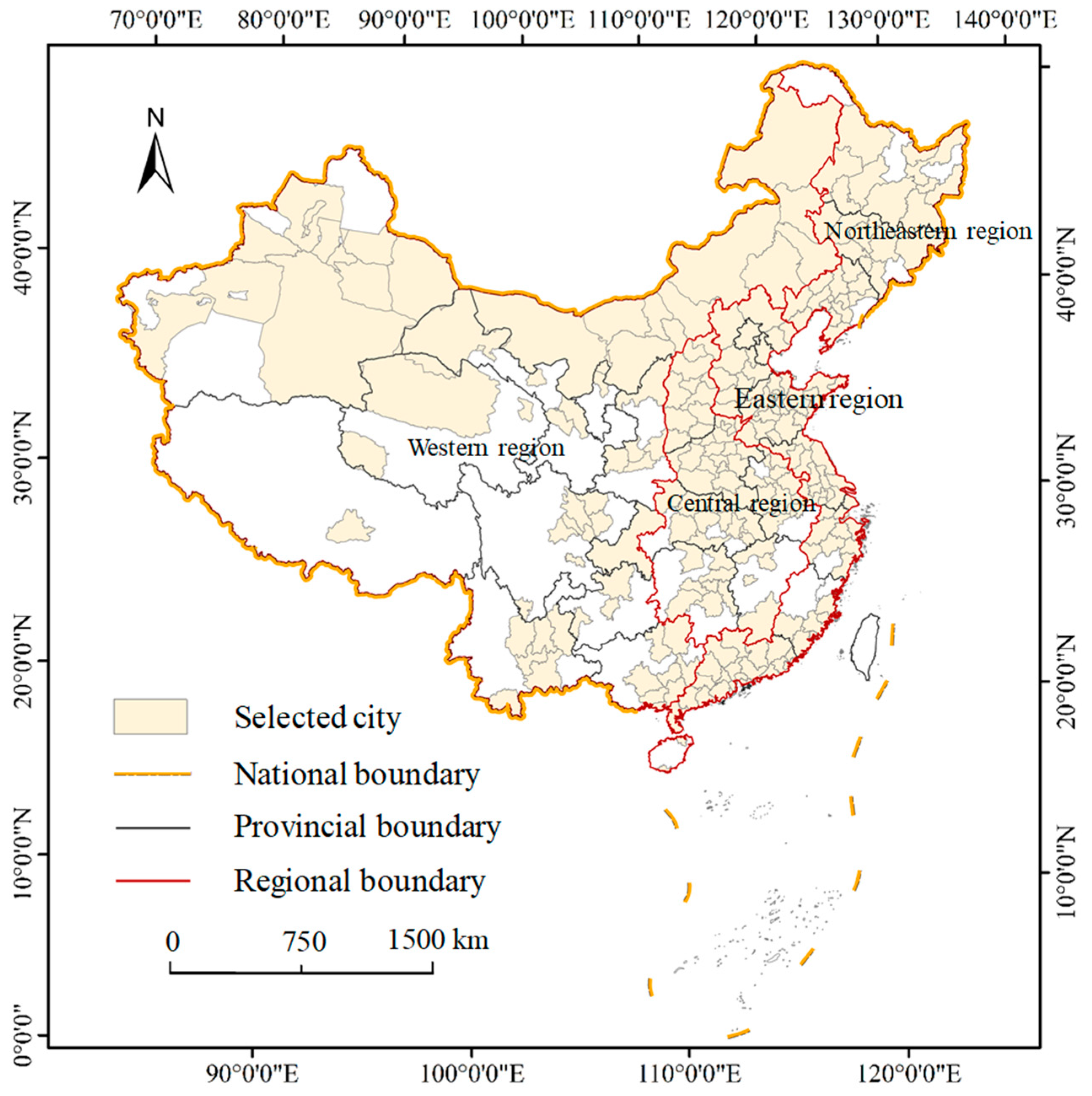
2.1. Study Area

The 241 prefecture-level cities in China were selected as case studies (Figure 2). China’s GDP and population have experienced amazingly rapid growth following reform and opening up, which has led to rapid urban expansion. China’s urban expansion shows serious regional disparity, which is manifested as regional disparities in urban spatial and socioeconomic growth. With the premise of ensuring data integrity, the 241 cities selected in this study were evenly distributed in the 31 provinces of China; specifically, 84 cities were in the eastern region (ER), 31 cities were in the northeastern region (NER), and 63 cities were in the central region (CR) and western region (WR). As there are economically developed cities and relatively poor cities in each region, we believe that these cities can be used to adequately analyze the regional dimensions of cities from the provincial level and region, as well as the differences between USS and USE within different regions.

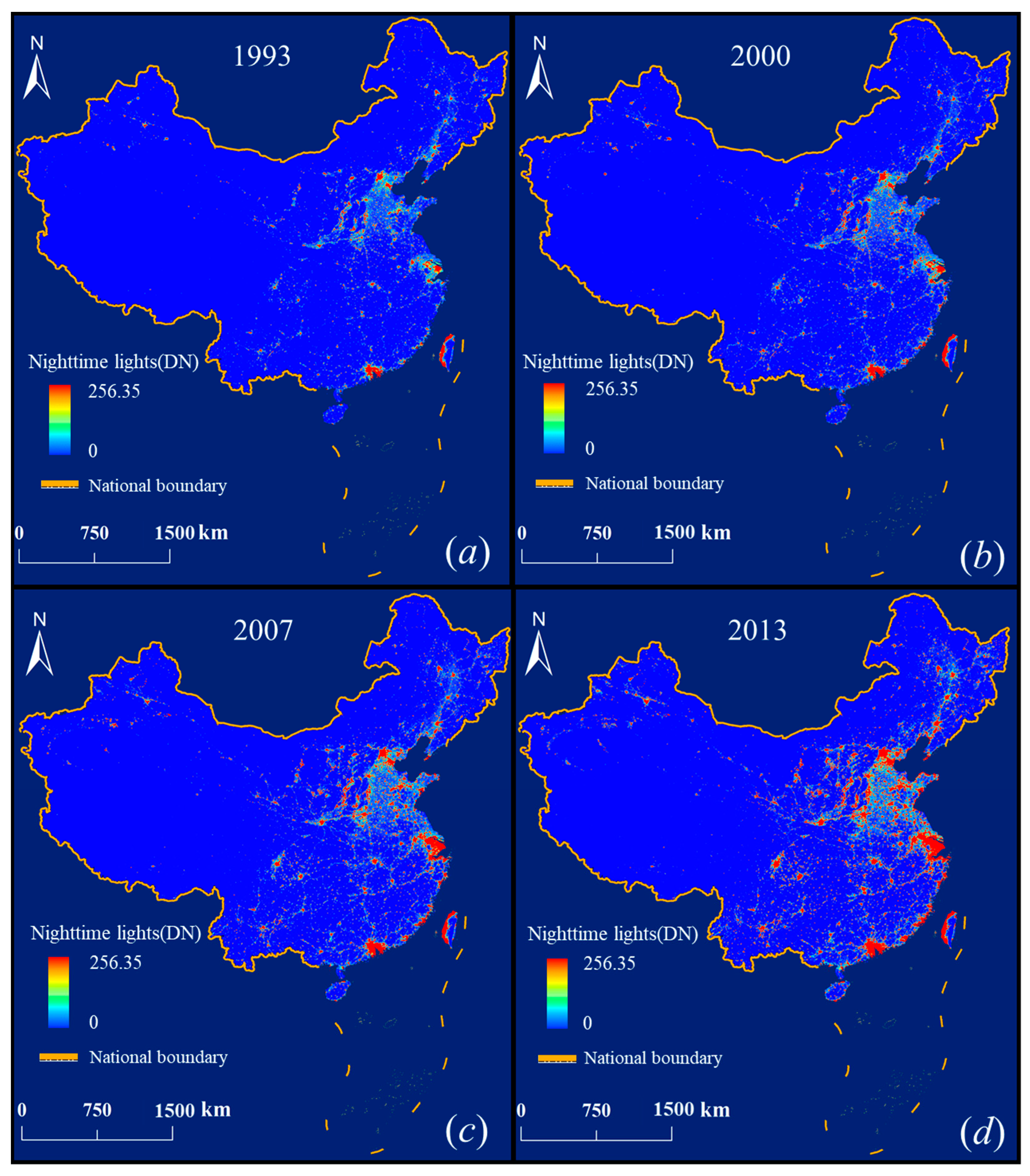
2.2. Data Sources and Data Processing

Two kinds of data were used to evaluate the regional disparity of urban expansion in China, including the urban land datasets, DMSP-OLS nighttime stable light (NSL) data, and collected urban land data, along with per capita GDP (PGDP) data from China Urban Statistical Yearbook (http://www.stats.gov.cn/tjsj/ (accessed on 19 April 2021)) for regression analysis to verify the accuracy of USS and USE.
Referring to the study by He et al. [20], urban land datasets were extracted by a hierarchical support vector machine (SVM) using the NTL data (https://ngdc.noaa.gov/eog/dmsp.html (accessed on 13 April 2021)), land surface temperature (LST) (http://ladsweb.nascom.nasa.gov (accessed on 13 April 2021)), and normalized difference vegetation index (NDVI) data (http://edc2.usgs.gov/ (accessed on 13 April 2021) and http://free.vgt.vito.be/origin (accessed on 13 April 2021)) from 1992 to 2015 (Figure 3) [21]. The data were projected to the equivalent region of the Albers cone and resampled to a 1 km resolution before processing. Fine-scale urban land data generated by Landsat data (http://www.geodata.cn/Portal/index.jsp (accessed on 14 April 2021)) were used to verify the accuracy of the extraction results, with the average Kappa value reaching 0.66 [22], which illustrated that reliable information from the datasets produced by He et al. [20] could quantify the spatial dynamics of urban land expansion in China.
The NSL data were collected from the National Geophysical Data Center of the US National Oceanic and Atmospheric Administration (https://ngdc.noaa.gov/eog/dmsp.html (accessed on 12 April 2021)). The NSL data exclude erratic lights that do not derive from cities, towns, or other sites of human activity. The digital number (DN) of the data was six bits (i.e., 0–63), with a spatial resolution of thirty arc-seconds (approximately 1-km). However, the NSL data have two flaws: (1) DN oversaturation, and (2) lack of continuity and comparability. Thus, this study adopted the method developed by Shi et al. [23] to process the NSL data; the corrected NSL data from 1993–2013 are shown in Figure 4.

3. Methods

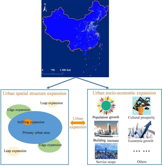
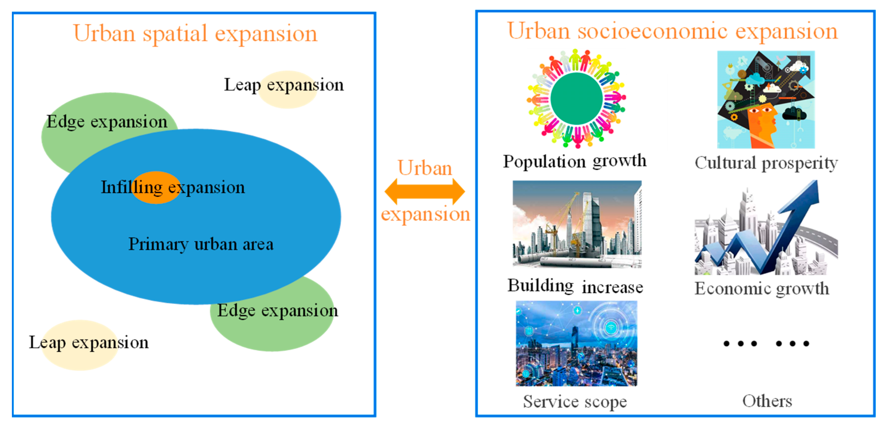
3.1. Defining Urban Expansion

The urban land datasets and NSL data were used to quantify USS and USE, respectively, in order to reflect the extent of urban expansion and intensive urban development. Following to Chen et al. [24], two comprehensive indexes, U1 and U2, were used to represent USS and USE, respectively, for evaluation in this study. The formulas are as follows:
U 1 = S A
U 2 = i = s l × DN i n i N × l
where U1 represents the USS, S is the built-up area of a specific city in urban land datasets, and A is the city’s administrative area. U2 represents the USE, DNi is the i-th gray value of the NSL data, ni is the number of pixels of the i-th gray value in the NSL data, l is the highest DN value in the study area, s is the lowest DN value in the study area, and N is the total number of bright pixels in the NSL data (lDNs).

3.2. Calculating Dagum Gini Coefficient

The DG coefficient can decompose the total regional development gap into the gaps formed by different sources in order to analyze the impact of different subsamples on overall regional differences. We selected the DG coefficient to measure the interval gap and analyze the disparity in urban expansion of the four plates and at the provincial level in three parts: regional differences, regional differences, and the super-variable density. The development differences between them and their respective contributions to the overall regional differences were compared from the two aspects of USS and USE. Moreover, the DG coefficient and its method of subgroup decomposition effectively solve the problem of cross-overlap among subsamples [25]. The Gini coefficient is defined as follows:
G = j = 1 k h = 1 k i = 1 n j r = 1 n h | y ji y hr | 2 n 2 y ¯
where G is the overall Gini coefficient, y ¯ is the average value of urban expansion (USS or USE), n is the number of provinces, k is the number of regional divisions, y ji   ( y hr ) is the urban expansion value of any province in j (h) regions, n j   ( n h ) is the number of provinces in j (h) regions, j h is the number of regional divisions, and j h is the number of provinces in the region.
The Gini coefficient can be divided into three parts: the contribution G w of regional difference, the contribution G nb of regional gaps, and the contribution G t of super variable density. The relationship between them satisfies G = G w + G nb + G t . Formulas (4) and (5) represent the Gini coefficient G jj of region j and contribution G w of intraregional difference, respectively, while Formulas (6) and (7) represent the contribution of Gini coefficient G jh between regions j and h and the contribution of the over-variable net worth gap G nb between regions, respectively. Finally, Formula (8) represents the contribution of over-variable density G t .
G jj = 1 2 Y j i = 1 n j r = 1 n j | y ji y jr | n j 2
G w = j = 1 k G j j p j s j  
G j h = i = 1 n j r = 1 n h | y j i y h r | n j n h ( Y j ¯ + Y h ¯ )  
G nb = j = 2 k h = 1 j 1 G jh ( p j s h + p h s j ) D jh
G t = j = 2 k h = 1 j 1 G jh ( p j s h + p h s j ) ( 1 D jh )
where p j   = n j Y ¯ , s j = n j Y j ¯ n Y ¯ , j = 1, 2, …, k; D jh is the relative influence of urban expansion between cities j and h, and its definition is shown in Formula (9); djh is the difference in urban expansion between cities, and its definition is shown in Formula (10), which can be understood as the mathematical expectation of the sum of all y ji y hr > 0 sample values in regions j and h; and p jh is defined as the first-order moment of super transformation, which represents all yhr in cities j and h. The sample value of y hr y ji > 0 summed to the mathematical expectation.   F j   ( F h ) is the cumulative density distribution function of the j (h) city.
D jh = d jh p jh d jh + p jh
d jh = 0 dF j ( y ) 0 y ( y x ) dF h ( x )
p jh = 0 dF h ( y ) 0 y ( y x ) dF j ( x )  

3.3. Stochastic Convergence Test

As an important method of convergence testing, the stochastic convergence method can test whether one variable has a continuous impact on another variable, which is information that can be used to avoid the possible state between convergence and non-convergence in the short term. The unit root test proposed by Carlino et al. [26] and Evans et al. [27] has been widely used in various studies. According to the results of the test, if there is a unit root, then the urban expansion is divergent between regions; otherwise, if there is no unit root, then the urban expansion is convergent between regions.
Following to the study of Carlino et al. [26], we assumed that the USS and USE of each city can be attributed to their respective compensation difference equilibrium level, which does not change with time in the long term. Then, the USE and USS of a city at time t can be written as the sum of USEe (USSe) and ut, as shown in Formula (12), where the former represents the average that does not change with time and the latter represents the deviation of the data value from the equilibrium level.
USE t ( USS t ) = USE e ( USS e ) + u t
u t   = v 0 + β t + v t
For the existence of transport condition convergence, it is assumed that neither USEe or USSe is 0. When the convergence hypothesis in Baumol’s research is dynamized, ut can be decomposed into a deterministic linear trend and a stochastic process. In Formula (13), v 0 represents the initial deviation of the data value from the equilibrium level and β t represents the deterministic convergence rate. By substituting Formula (13) into Formula (12), we obtain
USE t ( USS t ) = α + β t + v t
Evans and Karras’ approach is essentially the same as that of Carlino et al. [26,27]. First, if the common trend α t and a finite number of parameters μ 1 , μ 2 , , μ n make Formula (15) valid, then the urban expansion of these N units converges. Among them, n = 1, 2, …, N; y n t is the USE and USS of the n units in period t; and α t is the common trend of urban expansion of all units.
l i m i E t ( y n , t + i α t + i ) = μ n
l i m i E t ( y ¯ t + i α t + i ) = 1 N n = 1 N μ n
l i m i E t ( y ¯ n , t + i y ¯ t + i ) = μ n
Because α t is not observable, Formula (14) cannot be used, and α t must be eliminated. The method is thus to average Formula (14) and obtain Formula (15), of which y ¯ t = n = 1 N y nt / N . As we measure the common trend, α t , the right side of Formula (15) is equal to 0, and we can subtract Formula (15) from Formula (14) to obtain Formula (17). According to Formula (16), for each economic unit n = 1, 2, …, N, if and only if y nt y ¯ t is a stationary sequence, there is a convergence trend for the N units:
( y nt y ¯ t ) = δ n + ρ n ( y n ,   t 1 y ¯ t 1 ) + i = 1 p φ ni ( y n , t i y ¯ t i ) + u nt
Under this definition, whether convergence occurs can be determined by whether the autoregressive parameter ρ n in Formula (17) is zero. In Formula (18), if the units are convergent, then ρ n is negative; however, if the units are divergent, then ρ n is equal to zero. In addition, δ n and φ ni are parameters that make up all the roots of i φ ni L i outside the unit circle, L is a lag operator, and assuming that N tends to infinity, all u values in Formula (13) are unrelated. Therefore, testing random convergence becomes testing whether y nt y ¯ t is stable. If y nt y ¯ t is a stable sequence, the external shock effect is temporary and gradually dissipates over time, eventually making the economic development of the nth unit tend to a common trend. In contrast, if y nt y ¯ t is a nonstationary sequence, the external shock effect persists and eventually causes urban expansion deviate from the common trend.

4. Results and Discussion

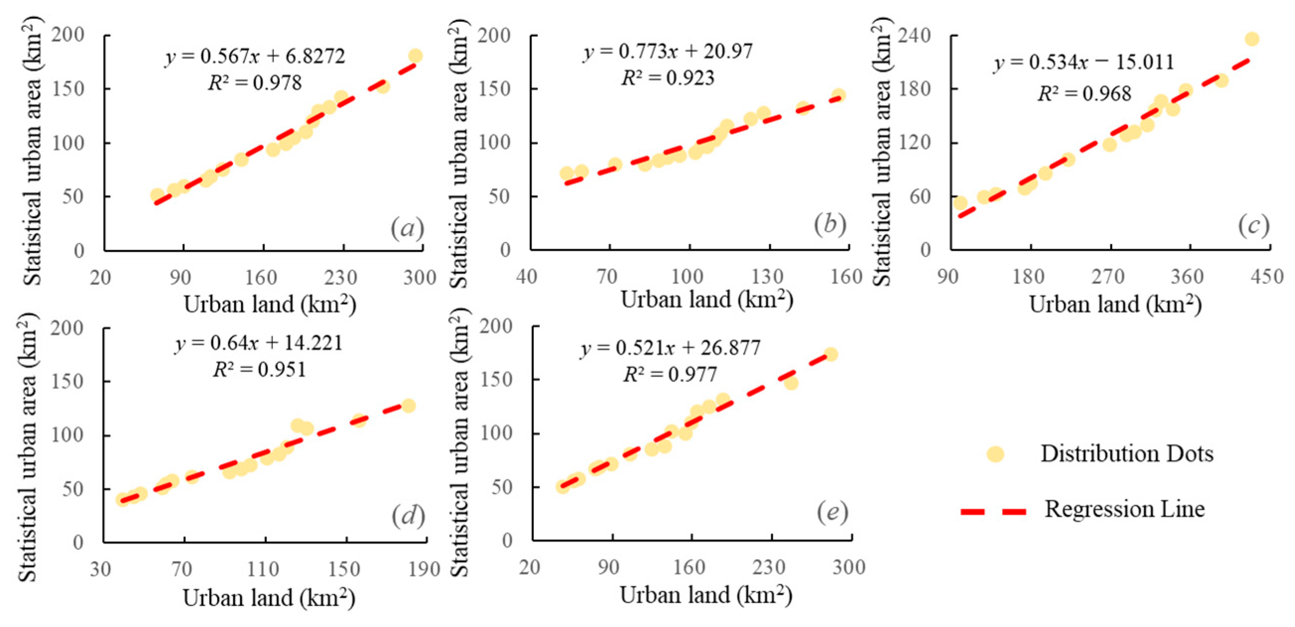
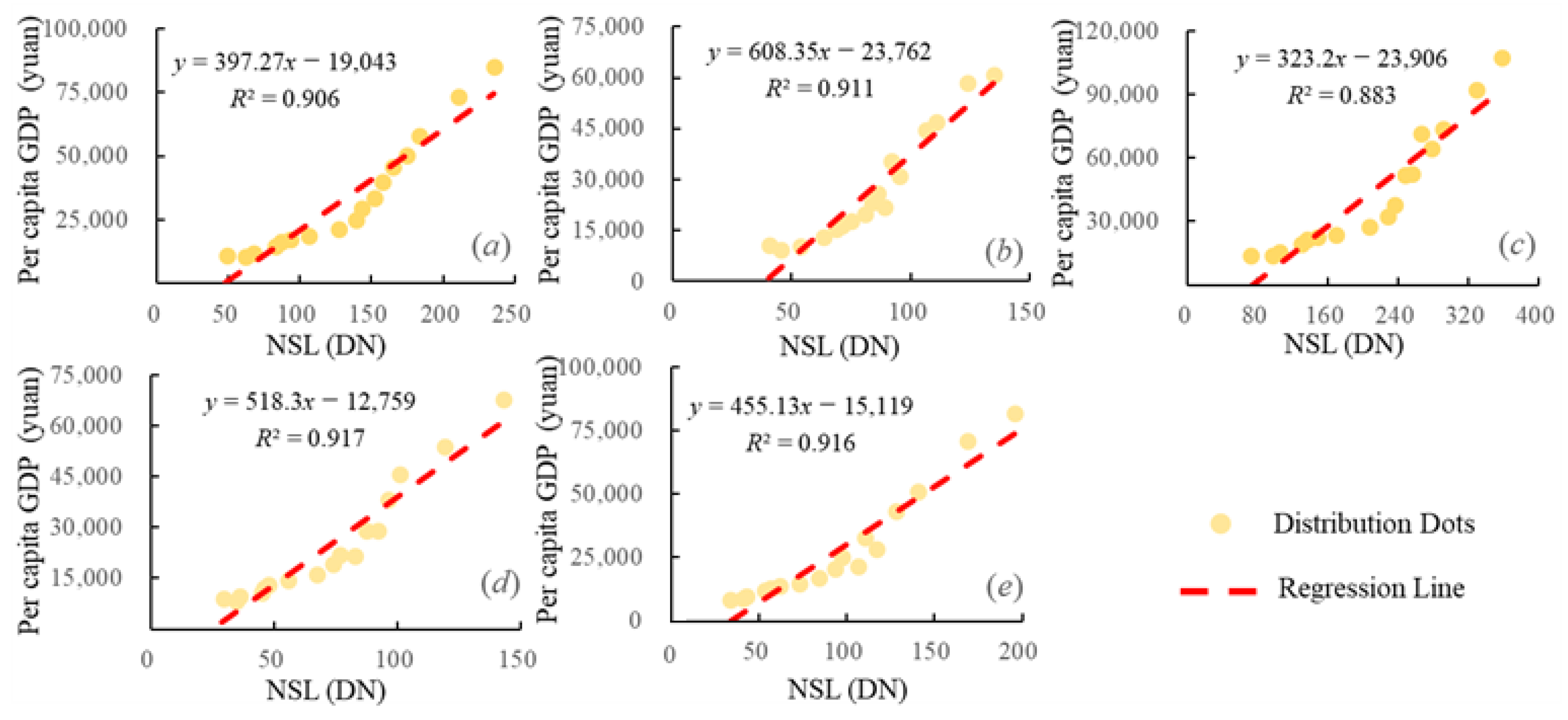
4.1. Accuracy Evaluation of Urban Expansion

To verify the accuracy of USS and USE, urban land data and per capita GDP (PGDP) data were collected from the China City Statistical Yearbook [28] and linear regression analysis was performed with urban land datasets and NSL data, respectively. The results are shown in Figure 5. On the national scale, the correlation coefficient (R2) value reached 0.978. At the regional scale, the R2 values of the NER, ER, CR, and WR were 0.923, 0.968, 0.951, and 0.977, respectively. These results correspond to the accuracy evaluation results of He et al. [20,23] and Shi et al. [20,23], indicating that the urban land data extracted by the SVM model can be used to adequately show the USS in China.
In terms of the accuracy of the USE from the NSL data (Figure 6), the R2 value of PGDP reached 0.906 within all cities. On the regional scale, the R2 value in the NE was 0.911, the R2 value in the ER was 0.883, in the CR it was 0.917, and in the WR it was 0.916, all of which are at relatively high levels and can effectively replace traditional statistical data such as PGDP. The results indicate that the NSL data have a simple processing method, can accurately reflect the urban economic activity [29], and represent a simple, rapid, and effective data source for the evaluation of USE. In summary, the regression analysis shows that urban expansion constructed by urban land data and NSL data have good accuracy and can be good substitutes for traditional data for the analysis of regional urban expansion.

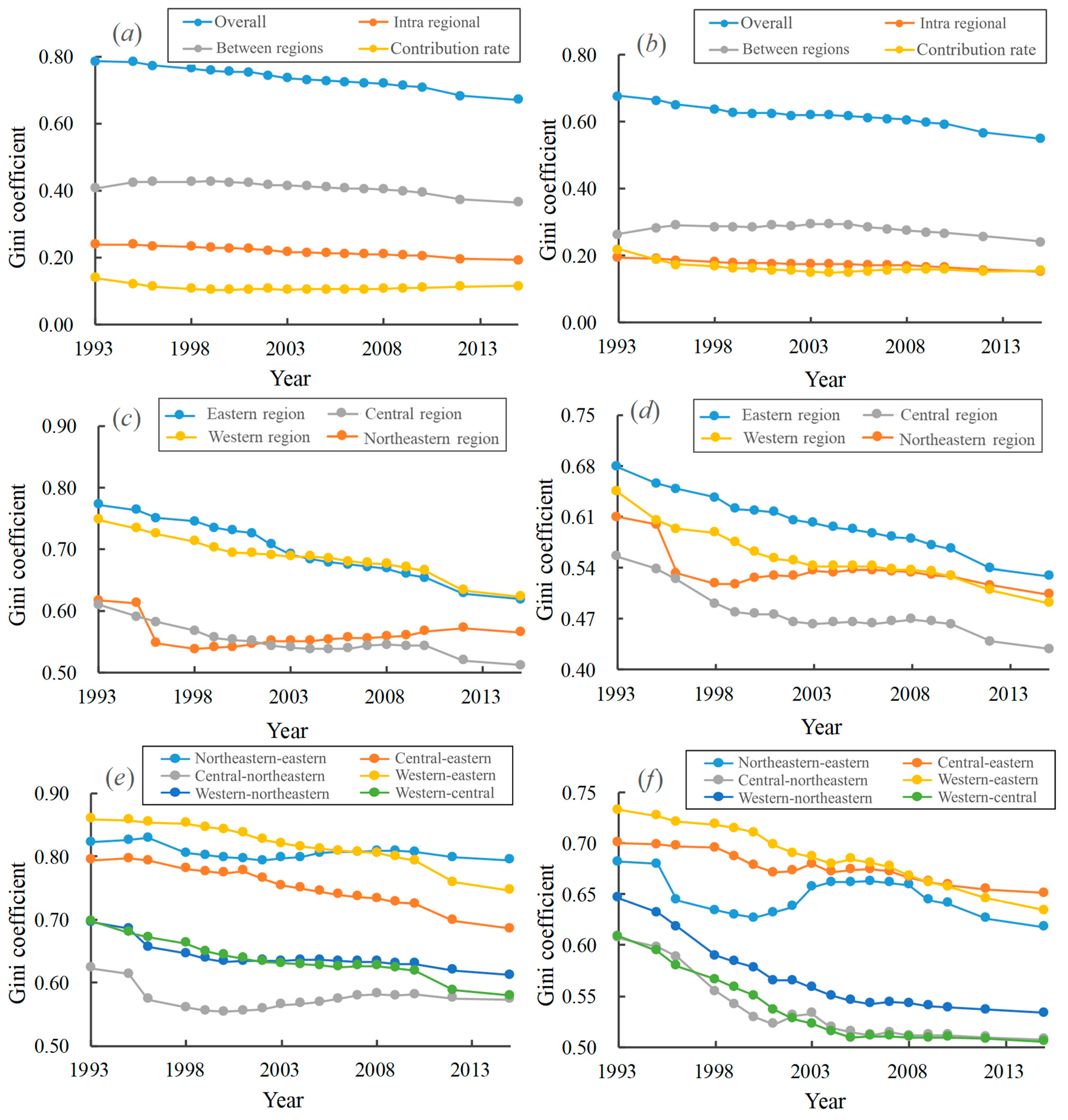
4.2. Regional Disparity in Urban Expansion in China

As shown in Figure 7, the overall regional disparity has gradually decreased in both the level of USS and the level of USE, indicating that China has continued to develop its economy over the long period since 1978 and the gap in urban development has continued to narrow. However, there are significant spatial non-equilibrium features. Table 1 shows that the DG coefficient of USS in 2015 was 0.670, while the corresponding DG coefficient of USE in Table 2 was 0.550. Economically, there are large differences between different cities. However, based on the rate of decline in regional differences, the DG coefficient of USS has declined by an average of 0.523% per year. Among them, the decline rate was faster than the average from 1995 to 1996, 2001 to 2003, and 2010 to 2012. This difference is due to factors such as the 1995 strict control of the scale of fixed-asset development, the control of land leases, the large area of land requisitioned between 2002 and 2003 [30], and the “Eleventh Five-Year Plan” mid-west development policy, which caused these trends. By standardizing the use of urban land and improving the land contract system, the marketization and commercialization of real estate was accelerated in large, medium, and small cities, which supported urban construction in less developed areas in the central and western regions and improved the efficiency and benefit of urban land use. The urban land area has accelerated, and the gap has decreased [31]. According to Table 2, the level of USE shows that the DG coefficient decreased from 0.677 in 1993 to 0.550 in 2015, an average annual decrease of 0.577%, which was greater than the average annual decline of USS (0.523%). This result indicates that, at the national scale, the difference in USE is smaller than that of USS and the development convergence of USE is higher than that of USS. This result is not inconsistent with the conclusion that the USS rate of Chinese cities in a previous study was much higher than the USE rate. The uneven development rate has led to differences in the development of different urban land areas and the level of economic expansion. The mobility of labor factors in economic activities as well as the government’s active regional coordinated development policy indicate that the differences in USE will continue to decrease [32]. In addition, the evolution of USE during the study period had a certain degree of volatility. For example, the DG coefficient fell to 0.624 in 2000, increased to 0.625 in 2001, and declined to 0.618 in 2002. In 2003, the value increased to 0.621, after which the regional differences showed an overall downward trend related to the international background at the time. For example, China’s accession to the WTO in 2001 enabled several cities to expand their overseas markets [33], and the development of SARS in 2003 affected normal production in most cities [34].

4.3. Decomposition of Regional Disparity in Urban Expansion

Using the subgroup decomposition method of the DG coefficient, the overall regional gap can be decomposed into three parts: the intraregional gap (Gw), the interregional gap (Gnb), and the hypervariable density contribution (Gt); thus, the contributions of different subsamples to the overall regional gap can be analyzed. Therefore, this study used the DG coefficient to decompose by subgroup based on the spatial scale of the four major regions in order to reveal the source of the overall regional urban expansion disparity in China. The results of the decomposition at the level of USS and USE are shown in Table 1 and Table 2, respectively, and Figure 8 visually depicts the overall regional disparity and the evolutionary trends of its components. From the measurement results, it can be seen that the intraregional gap, interregional gap, and hypervariable density contributions are roughly decreasing, and most of China’s overall regional gap can be explained by the overall differences in USS and USE between different regions [35]. While the regional differences and the overlapping of different regions have an impact on the overall gap, no regional differences have a large impact, especially in terms of the economic aspect, which shows that the impact of regional overlapping on economic development is greater than the impact of urban land areas. That is, the influence of regional factor flow is greater than the scale of development of urban differentiation. This pattern is reflected in research by Liang et al. [36]. Labor, capital, and technological factors are concentrated in certain cities in the ER, where the economy has developed rapidly. At the same time, this process promotes USS, and the situation limits the areas where these factors are exported, such as the NER and CR; as a result, the cities in these regions cannot be effectively developed as there is no economically developed metropolis, resulting in the Gini coefficients being among the lowest within or between these regions. The WR is a sparsely populated area. Due to a large number of residents and large amount of industry and commerce in the cities, most cities have poor natural conditions, inconvenient transportation, and overpopulation problems. These conditions lead to differences in economic development [37]. In the economically developed ER, the phenomenon of the largest regional differences shows that the eastern cities have had the greatest differences, that is, there is a concentrated development of major cities, which promotes the development of the local economy in the short term. However, it hinders the economic development of neighboring areas, and thus there is a large difference between USS and USE. With the introduction of various policies implemented by the Chinese government for coordinated development [38] this phenomenon is being broken, as reflected in the continuous decline of regional differences in the study area.
In terms of intraregional differences (Figure 9), the evolutionary trend of the urban expansion Gini coefficient in the NER was not stable, showing a “U”-shaped change. The value of the Gini coefficient decreased significantly compared to that in 1995. This phenomenon occurred because the NER is a high-latitude region. Although there may be irradiance errors during NTL data collection and processing, this does not affect our research on its trends. In general, the regional urban expansion disparity in the four regions is decreasing. Among the regions, the unbalanced phenomenon of USS in the ER is more significant than that in the other three regions. The Gini coefficient of USS and USE is the highest, followed by that in the WR; furthermore, the NER is more balanced, and the CR is the most balanced. Moreover, only the gap between the USS and the level of USE in the ER is decreasing, and the regression coefficient is −0.0009, which shows that with the deepening of the reform and opening up policies, the coordinated development of cities in the ER has achieved remarkable results. The trend of the coordinated development of USE and USS is obvious, while the other three regions show that the difference in USE is smaller than that in USS. The difference regression coefficient is 0.0005 in the WR, 0.0012 in the CR, and 0.0022 in the NER; the difference in the NER is most significant. This result shows that in terms of the sustainable development of cities there are obvious differences in development in the NER, which is consistent with the shrinkage of cities in the NER in recent years. However, the Chinese government has promoted the development of certain cities in its strategy of revitalizing the NER, which has led to an increase in USS [38], while the difference in USE has changed from large to small. Due to the massive loss of labor factors in the central and western cities, capital and technological factors have been lost to the eastern cities, resulting in slow development between 2000 and 2010. In contrast, due to policy support in CR, although the level of USS is slow, the level of USE has achieved results and the socioeconomic gap within the region has gradually decreased.
In terms of interregional differences (Figure 10), the regional USS and USE disparities are both decreasing, and the differences are the largest in the ER, WR, NER, and CR, in order, which is reflected in the study of the Gini coefficient of the USS between regions. During the study period, all values were above 0.686 and the Gini coefficients between the socioeconomic regions were above 0.583, indicating that the weight of USE remains concentrated in the eastern coastal area. Furthermore, economic development has led to urban construction, separating the east from the remaining three regions [39]. In contrast, the disparities between NER–ER, CR–NER, and WR–NER are almost unchanged at the USS level, and there are large differences in USE between the latter two. The k values of the regression analysis are 0.0039 and 0.0023, respectively, indicating that during the period under investigation the disparity in urban expansion continued to exist for the remaining three regions, and that the relative decline of urban expansion has not been effectively contained. However, due to the redevelopment of heavy industry, the regional economic plan has stimulated the socioeconomic level, which has caught up with the development of other regions, continuously narrowing the gap. The trend of reduced Gini coefficients in the CR and ER shows that the CR is being driven by the influence of the ER, and the phenomenon of the USS and USE converging appears in the ER. However, due to the labor factors mentioned above, the flow has caused the trend in USS to move faster than USE, and there has been a situation where the difference between USS and USE has narrowed [40]. The same situation occurs in the regional differences between the CR and ER. The narrowing of the gap between the WR and CR has benefited from the early implementation of the western development plan, which has narrowed the gap between the WR and CR. Of course, at present, the Chinese government has launched a strategic policy of national land spatial planning and regional coordinated development [39], and the differences in horizontal and vertical development of the four major regions will gradually narrow.
From the perspective of contribution (Figure 11), the differences between different regions in China are the main source of the imbalance between USS and USE, which has the greatest impact on the level of USS, with its relative contribution more than half. The expansion level reaches a contribution of 38–49%, which is consistent with the results above. Specifically, at the USS level, the contribution of the intraregional gap decreased from 30.486% in 1993 to 28.543% at the end of 2015, which was higher than the USE level of 28.806% at the beginning of the period and 27.852% at the end of the period. These degrees are relatively balanced, indicating that the urban development in each region has differences in USS and USE and the different levels are similar. The differences among regions all show an inverted “U” trend, and their contribution is the largest in the vicinity of 2003. The contributions of their USS regions were 56.422% in 2003 and 47.559% in 2004. Combined with the above analysis, we can see that in the 1990s several developed cities, especially the eastern coastal areas and western industrial cities, had particularly rapid development after reform, opening up, and market economy reform; after entering the 21st century, China’s USS and USE have shown a trend of coordinated development, causing the gap to move toward convergence [40]. While the difference between USS and USE has reached approximately 10%, it shows a shrinking trend, which further shows that the flow of regional factors is very significant in China. Many regional laborers live in a certain area due to the restriction of household registration, and the phenomenon of production work in other regions is still widespread. Of note is the degree of contribution of hypervariable density. The degree of contribution to USE exceeds the degree of contribution to spatial expansion. Contrary to the difference between regions, the degree of contribution is “U”-shaped. This trend may be due to the large-scale concentration of China’s economy in certain cities, such as the Beijing–Tianjin region [12], the Yangtze River Delta region [41], and the Pearl River Delta region. These places bring together a large population and capital, making city construction faster than in other regions. The difference between USS and USE is reflected in this circumstance. Although the current trend of the two has been shrinking and the regression slope of the difference is −0.1278, they both showed an upward trend after 2004. According to this trend, even if the development of Chinese cities in the general environment shows convergence, the external economic phenomenon of the city will continue to appear [35].

4.4. Stochastic Convergence Test of Urban Expansion

To further explore the convergence of the USS and USE levels, the panel unit root test method was used to conduct empirical tests on the convergence of the two dimensions of China’s urban expansion, following the full subset analysis path to examine the existing spatial expansion and the convergence club of economic development. Panel unit root test methods such as the IPS test for the null hypothesis, in which all sequences have unit roots, and the stationary Hadri test for all sequences were used. Compared with the univariate unit root test, the interpretation of the panel unit root test results was ambiguous. All series are stationary and do not mean that the IPS test rejects the null hypothesis; additionally, the presence of unit roots in all series did not support the Hadri test. The test rejects the original hypothesis, which is bound to affect the reliability of the results when using only a single indicator as the test standard. Here, according to confirmative analysis (CA) from the studies of Liu [40] and Choi [42], the comparison of different types of panel unit root test results was used to obtain a more reliable conclusion. Specifically, the following four cases appear in the confirmatory analysis: first, neither the IPS test nor the Hadri test rejects the null hypothesis, and the stability of the sequence cannot be judged at this time. Second, the IPS test does not reject the null hypothesis, and the Hadri test significantly rejects the null hypothesis. At this time, all sequences have unit roots, and the variables randomly diverge. Third, the IPS test rejects the null hypothesis, and the Hadri test does not reject the null hypothesis. At this time, all-time series can be regarded as stationary random processes, that is, there is random convergence between the variables. Fourth, both the IPS test and the Hadri test reject the null hypothesis, and the conclusion is not clear at this time because part of the sequence may randomly converge and part of the sequence may randomly diverge. The application of CA can make the panel unit root test results more rigorous and improve the credibility of the results. Therefore, this study combines CA with the determination of whether there is random convergence in the two dimensions of China’s urban expansion, i.e., the USS and USE levels.
Starting from the investigation of the existence of a nationwide stochastic convergence trend, first, the natural logarithm values of the USS dataset and USE dataset of the city were sampled, then panel unit root tests were conducted at the national scale and in the four major regions. Table 3 shows that the CA results are the second result in both the USS level and the USE level in the country and the four major regions. Even at a significance level of 10%, the IPS test cannot reject the null hypothesis of the existence of unit roots, and the Hadri test significantly rejects the stationary null hypothesis. The CA results show that there is random convergence within some regions regardless of USS and USE in the development of Chinese cities; there is a possibility of differentiation, and one or more convergence clubs will be formed in the future. Through comparative analysis, we can see that the USE in the study sample area, specifically the NER and ER, has a trend of more stable development than the USS.
This study further used univariate unit root test methods such as ADF and KPSS to examine the random convergence trends of USS and USE in samples from 31 provinces to determine whether certain provinces converge with the national mean range. The results are listed in Table 4. According to the ADF test results, a total of six provincial USS sequences and five provincial USE sequences rejected the original hypothesis of unit roots, while the other provinces accepted the original hypothesis. Among them, for USS, Shanxi rejected the existence of unit roots at the 1% significance level. At the 5% significance level, there were two provinces, Guangdong and Guangxi, while at the 10% significance level, there were three provinces, Tianjin, Heilongjiang, and Ningxia. For USE, there were three provinces at the 5% significance level, Anhui, Hebei, and Qinghai, and two provinces at the 10% significance level, Guizhou and Shaanxi.
According to the KPSS test results, among all 31 provinces and cities, 20 provinces rejected the original hypothesis of stationarity of the USS sequence while 20 provinces rejected the original hypothesis of stationarity of the USE sequence. Among them, 18 cities rejected both sequences, while Hebei and Qinghai rejected only the original hypothesis that the USS sequence was stable and Ningxia and Xinjian only rejected the original hypothesis of USE. Under the premise of global random divergence, there may be random convergence of economic development in certain regions. Global random divergence does not negate the possibility of the existence of a subset of convergence.

5. Conclusions

This study has attempted to define urban expansion from the USS and USE, respectively. Through the multiscale analysis of 241 prefecture-level cities within different provinces and four major regions in China from 1993 to 2015, we analyzed and compared regional disparities in urban expansion in China. Using the method of factorization of the DG coefficients by subgroup, the differences between rapid USS and USE as well as between different regions were analyzed from the overall gap, the contributions of intraregional, interregional, and hypervariable density, and the relationship between USS and USE at different scales. Finally, the global club test was used to verify the random convergence phenomenon of Chinese urban expansion through the panel unit root test. The results showed that the overall regional urban expansion disparity in China can be explained by the overall differences in USS and USE between different regions. The contributions of the interregional and intraregional differences and the hypervariable density decreased in sequence. The impact of the first two items on economic development was less than that of urban land areas, and the hypervariable density was opposite; specifically, the difference in overall USS in China was greater than the difference in USE. On the regional scale, the difference was the largest in the WR, followed by the ER and CR, and the difference was the smallest in the northeast region. Except for the ER, the difference between USS and USE in the other three regions was expansionary, and the difference between regions was the main source of unevenness in USS and USE. This difference was the largest in the ER and WR, then the the NER and CR, followed by the other regions, although the difference in USS in the NER showed a relatively widening trend. The difference between USS and USE showed a shrinking trend, that is, USS is converging on a large scale; however, in the future there will be external non-economic urban phenomena. The results of the global club test showed that there was random convergence within certain regions regardless of the USS level and USE level in the development of Chinese cities; there is a possibility of differentiation, and one or more convergence clubs will be formed in the future. The trend of stochastic convergence on the provincial scale indicates that under the premise of global random divergence there may be random convergence of economic development in certain regions, and global random divergence does not negate the possibility of a subset of convergence.
It is undeniable that there are several aspects worthy of further exploration following this study. First, the time coverage of DMSP-OLS data has only been updated to 2013, limiting its application after 2013. As the successor to DMSP-OLS data, NPP-VIIRS data has been released since 2012 and is being updated. Thus, the integration of DMSP-OLS and NPP-VIIRS data to remeasure regional disparities could improve the reliability of conclusions in future urban planning. Second, as the Dagum Gini coefficient cannot consider the regional difference from the spacing effect or delve into the mechanism of urban expansion disparity, it is necessary to further employ the distance function to measure the overall performance of urban expansion in the future.

Author Contributions

Z.C.: Writing-Original draft preparation, Methodology, Validation, Editing. S.L.: Validation. Editing. Y.W.: Validation, Editing. K.S.: Conceptualization, Methodology, Supervision, Editing. All authors have read and agreed to the published version of the manuscript.

Funding

This research was funded by the National Natural Science Foundation of China (42101345) and the Chongqing Social Science Planning Project (2021NDQN39).

Data Availability Statement

Not applicable.

Conflicts of Interest

The authors declare no conflict of interest.

References

  1. Bai, X.; Shi, P.; Liu, Y.J.N. Society: Realizing China’s urban dream. Nature 2014, 509, 158–160. [Google Scholar] [CrossRef]
  2. Gong, P.; Li, X.; Zhang, W.J.S.B. 40-Year (1978–2017) human settlement changes in China reflected by impervious surfaces from satellite remote sensing. Sci. Bull. 2019, 64, 756–763. [Google Scholar] [CrossRef]
  3. Shi, L.; Zhang, Z.; Liu, F.; Zhao, X.; Wang, X.; Liu, B.; Hu, S.; Wen, Q.; Zuo, L.; Yi, L.; et al. City size distribution and its spatiotemporal evolution in China. Chin. Geogr. Sci. 2016, 26, 703–714. [Google Scholar] [CrossRef]
  4. United Nations. About the Sustainable Development Goals. 2016. Available online: https://www.un.org/sustainabledevelopment/sustainable-development-goals/ (accessed on 20 May 2021).
  5. Zhang, X.; Brandt, M.; Tong, X.; Ciais, P.; Yue, Y.; Xiao, X.; Zhang, W.; Wang, K.; Fensholt, R. A large but transient carbon sink from urbanization and rural depopulation in China. Nat. Sustain. 2022, 5, 321–328. [Google Scholar] [CrossRef]
  6. Zhao, J.; Xiao, Y.; Sun, S.; Sang, W.; Axmacher, J.C. Does China’s increasing coupling of ‘urban population’ and ‘urban area’ growth indicators reflect a growing social and economic sustainability? J. Environ. Manag. 2022, 301, 113932. [Google Scholar] [CrossRef]
  7. Shi, K.; Wu, Y.; Liu, S. Does China’s City-Size Distribution Present a Flat Distribution Trend? A Socioeconomic and Spatial Size Analysis From DMSP-OLS Nighttime Light Data. IEEE J. Sel. Top. Appl. Earth Obs. Remote Sens. 2021, 14, 5171–5179. [Google Scholar] [CrossRef]
  8. Du, P.; Hou, X.; Xu, H. Dynamic Expansion of Urban Land in China’s Coastal Zone since 2000. Remote Sens. 2022, 14, 916. [Google Scholar] [CrossRef]
  9. Bernt, M. The limits of shrinkage: Conceptual pitfalls and alternatives in the discussion of urban population loss. Int. J. Urban Reg. Res. 2016, 40, 441–450. [Google Scholar] [CrossRef]
  10. Liu, S.; Shen, J.; Liu, G.; Wu, Y.; Shi, K. Exploring the effect of urban spatial development pattern on carbon dioxide emissions in China: A socioeconomic density distribution approach based on remotely sensed nighttime light data. Comput. Environ. Urban Syst. 2022, 96, 101847. [Google Scholar] [CrossRef]
  11. Wu, Y.; Li, C.; Shi, K.; Liu, S.; Chang, Z. Exploring the effect of urban sprawl on carbon dioxide emissions: An urban sprawl model analysis from remotely sensed nighttime light data. Environ. Impact Assess. Rev. 2022, 93, 106731. [Google Scholar] [CrossRef]
  12. Li, X.; Gong, P.; Liang, L. A 30-year (1984–2013) record of annual urban dynamics of Beijing City derived from Landsat data. Remote Sens. Environ. 2015, 166, 78–90. [Google Scholar] [CrossRef]
  13. Liu, S.; Shi, K.; Wu, Y.; Chang, Z. Remotely sensed nighttime lights reveal China’s urbanization process restricted by haze pollution. Build. Environ. 2021, 206, 108350. [Google Scholar] [CrossRef]
  14. Shi, K.; Chang, Z.; Chen, Z.; Wu, J.; Yu, B. Identifying and evaluating poverty using multisource remote sensing and point of interest (POI) data: A case study of Chongqing, China. J. Clean. Prod. 2020, 255, 120245. [Google Scholar] [CrossRef]
  15. Chen, Z.; Wei, Y.; Shi, K.; Zhao, Z.; Wang, C.; Wu, B.; Qiu, B.; Yu, B. The potential of nighttime light remote sensing data to evaluate the development of digital economy: A case study of China at the city level. Comput. Environ. Urban Syst. 2022, 92, 101749. [Google Scholar] [CrossRef]
  16. Zhao, M.; Cheng, C.; Zhou, Y.; Li, X.; Shen, S.; Song, C. A global dataset of annual urban extents (1992–2020) from harmonized nighttime lights. Earth Syst. Sci. Data 2022, 14, 517–534. [Google Scholar] [CrossRef]
  17. Pandey, B.; Joshi, P.K.; Seto, K.C. Monitoring urbanization dynamics in India using DMSP/OLS night time lights and SPOT-VGT data. Int. J. Appl. Earth Obs. Geoinf. 2013, 23, 49–61. [Google Scholar] [CrossRef]
  18. Shi, K.; Yu, B.; Huang, Y.; Hu, Y.; Yin, B.; Chen, Z.; Chen, L.; Wu, J. Evaluating the ability of NPP-VIIRS nighttime light data to estimate the gross domestic product and the electric power consumption of China at multiple scales: A comparison with DMSP-OLS data. Remote Sens. 2014, 6, 1705–1724. [Google Scholar] [CrossRef]
  19. Liu, Z.; He, C.; Zhang, Q.; Huang, Q.; Yang, Y.J.L. Extracting the dynamics of urban expansion in China using DMSP-OLS nighttime light data from 1992 to 2008. Landsc. Urban Plan. 2012, 106, 62–72. [Google Scholar] [CrossRef]
  20. He, C.; Liu, Z.; Tian, J.; Ma, Q. Urban expansion dynamics and natural habitat loss in China: A multiscale landscape perspective. Glob. Change Biol. 2014, 20, 2886–2902. [Google Scholar] [CrossRef]
  21. Cao, X.; Chen, J.; Imura, H.; Higashi, O. A SVM-based method to extract urban areas from DMSP-OLS and SPOT VGT data. Remote Sens. Environ. 2009, 113, 2205–2209. [Google Scholar] [CrossRef]
  22. Wang, H.; Liu, G.; Shi, K. What Are the Driving Forces of Urban CO2 Emissions in China? A Refined Scale Analysis between National and Urban Agglomeration Levels. Int. J. Environ. Res. Public Health 2019, 16, 3692. [Google Scholar] [CrossRef] [PubMed]
  23. Shi, K.; Chen, Y.; Yu, B.; Xu, T.; Yang, C.; Li, L.; Huang, C.; Chen, Z.; Liu, R.; Wu, J. Detecting spatiotemporal dynamics of global electric power consumption using DMSP-OLS nighttime stable light data. Appl. Energy 2016, 184, 450–463. [Google Scholar] [CrossRef]
  24. Chen, J.; Zhou, L.; Shi, P.; Ichinose, T. The Study on Urbanization Process in China Based on DMSP/OLS Data: Development of a Light Index for Urbanization Level Estimation. J. Remote Sens. 2003, 7, 168–175. [Google Scholar] [CrossRef]
  25. Liu, H.; Zhao, H.; Yang, Q. An Empirical Analysis on China’s Regional Disparity of Brand Economic Development and Its Influencing Factors: Based on Dagum’s Gini Coefficient Decomposition Method and China’s 500 Most Valuable Brands from 2004 to 2011. Econ. Rev. 2012, 3, 57–65. [Google Scholar]
  26. Carlino, G.; Mills, L. Testing neoclassical convergence in regional incomes and earnings. Reg. Sci. Urban Econ. 1996, 26, 565–590. [Google Scholar] [CrossRef]
  27. Evans, P.; Karras, G. Convergence revisited. J. Monet. Econ. 1996, 37, 249–265. [Google Scholar] [CrossRef]
  28. Press, C.S. China Statistical Yearbook. 2016. Available online: http://www.stats.gov.cn/tjsj/ (accessed on 19 April 2021).
  29. Wu, Y.; Shi, K.; Chen, Z.; Liu, S.; Chang, Z. Developing Improved Time-Series DMSP-OLS-like Data (1992–2019) in China by Integrating DMSP-OLS and SNPP-VIIRS. IEEE Trans. Geosci. Remote Sens. 2021, 60, 1–14. [Google Scholar] [CrossRef]
  30. Yang, S. Research on Governance of Real Estate Bubble from the Perspective of National Economic Security. Manag. Obs. 2015, 29, 13–73. [Google Scholar]
  31. Tan, Z.; Zhao, L. A Historical Analysis of the Process of the Great-leap-forward Development of West China. J. Yunnan Univ. Natl. 2013, 30, 101–107. (In Chinese) [Google Scholar]
  32. Fang, C.; Zeng, Z.; Cui, N. The economic disparities and their spatio-temporal evolution in China since 2000. Geogr. Res. 2015, 34, 234–246. (In Chinese) [Google Scholar]
  33. Chen, Z.; Song, P. WTO entry and the development of Chinese cities in the era of globalization. Urban Plan. Overseas 2002, 5, 1–2. [Google Scholar]
  34. Min, J. The Effect of the SARS Illness on Tourism in Taiwan: An Empirical Study. Int. J. Manag. 2005, 22, 497. [Google Scholar]
  35. Lu, H.; Ou, X.; Li, X.; Ye, L.; Sun, D. Space-Time Analysis on the Regional Economic Inequality and Polarization in China. Econ. Geogr. 2013, 33, 15–21. [Google Scholar]
  36. Liang, Q.; Chen, Q.; Wang, R. Household Registration Reform, Labor Mobility and Optimization of the Urban Hierarchy. Soc. Sci. China 2015, 36, 130–151. [Google Scholar]
  37. Ye, C.; Sun, C.; Chen, L. New evidence for the impact of financial agglomeration on urbanization from a spatial econometrics analysis. J. Clean. Prod. 2018, 200, 65–73. [Google Scholar] [CrossRef]
  38. Zhao, K.; Li, P.; Zhang, A. Impact of quality of economic growth on expansion of land use for urban construction: Perspective from total factor productivity. J. Huazhong Agric. Univ. 2012, 2, 53–57. (In Chinese) [Google Scholar] [CrossRef]
  39. Yang, B.; Xu, T.; Shi, L. Analysis on sustainable urban development levels and trends in China’s cities. J. Clean. Prod. 2017, 141, 868–880. [Google Scholar] [CrossRef]
  40. Liu, H.; Du, G. Regional Inequality and Stochastic Convergence in China. J. Quant. Tech. Econ. 2017, 34, 43–59. [Google Scholar] [CrossRef]
  41. Liao, C.J.; Huang, J.; Sheng, L.; You, H.Y. Grey Correlation Analysis between Urban Built-up Area Expansion and Social Economic Factors: A Case Study of Hangzhou, China. Appl. Mech. Mater. 2012, 209–211, 1615–1619. [Google Scholar] [CrossRef]
  42. Choi, C.-Y. A Variable Addition Panel Test for Stationarity and Confirmatory Analysis; Mimeo Department of Economics, University of New Hampshire: Durham, NH, USA, 2002. [Google Scholar]
Figure 1. Definition of urban expansion.
Remotesensing 14 04348 g001
Figure 2. Spatial distribution of the study area.
Remotesensing 14 04348 g002
Figure 3. Spatial distribution of urban land in China.
Remotesensing 14 04348 g003
Figure 4. Spatial distribution of the NSL data in China. 1993 (a), 2000 (b), 2007 (c), and 2013 (d). Note: according data availability, the 2015 NSL data were replaced by 2013 NSL data.
Remotesensing 14 04348 g004
Figure 5. Regression analysis between Urban land data and Statistical urban area. All cities (a), NER (b), ER (c), CR (d), and WR (e).
Remotesensing 14 04348 g005
Figure 6. Regression analysis between NSL data and PGDP. All cities (a), NER (b), ER (c), CR (d), and WR (e).
Remotesensing 14 04348 g006
Figure 7. The Dagum Gini coefficients of USS and USE. Note: USS is the urban spatial expansion and USE is the urban socioeconomic expansion.
Remotesensing 14 04348 g007
Figure 8. The results of the Dagum Gini coefficient; (a,b) are the overall Gini coefficient and contribution rate, respectively, (c,d) are intraregional, and (e,f) are between regions.
Remotesensing 14 04348 g008
Figure 9. Differences between USS and USE in different regions: (a) ER, (b) NER, (c) CR, and (d) WR. Note: USS is urban spatial expansion; USE is urban socioeconomic expansion.
Remotesensing 14 04348 g009
Figure 10. Differences between USS and USE between regions: (a) NER-ER, (b) CR-ER, (c) CR-NER, (d) WR-ER, (e) WR-NER, (f) WR-CR. Note: USS is urban spatial expansion, and USE is urban socioeconomic expansion.
Remotesensing 14 04348 g010
Figure 11. Differences between USS and USE contribution rates: (a) regional differences in contribution, (b) regional difference contribution, (c) ultra-variable density contribution. Note: USS is urban spatial expansion and USE is urban socioeconomic expansion.
Remotesensing 14 04348 g011
Table 1. DG coefficient and its decomposition of the USS.
YearOverall Regional DisparityIntra-RegionalBetween RegionsContribution Rate (%)
ERNERCRWRNER-ERCR-ERCR-NERWR-ERWR-NERWR-CRGwGnbGt
19930.7850.7720.6170.610.7470.8230.7940.6230.860.6960.69830.486 51.845 17.669
19950.7830.7630.6130.5910.7340.8290.7970.6130.8570.6860.68030.468 54.098 15.434
19960.7730.750.5480.5820.7250.8060.7930.5730.8540.6570.67130.312 55.061 14.627
19980.7640.7440.5380.5680.7130.7990.7810.5600.8520.6460.66230.278 55.713 14.009
19990.7580.7340.5400.5570.7020.7970.7760.5560.8460.6380.65030.158 56.307 13.535
20000.7540.7300.5420.5530.6940.7930.7730.5540.8430.6340.64330.096 56.309 13.595
20010.7530.7260.5460.5510.6930.7970.7770.5550.8370.6340.63830.031 56.094 13.876
20020.7420.7070.5510.5430.6900.7980.7650.5580.8270.6350.63329.730 55.961 14.310
20030.7340.6910.5510.540.6880.8050.7540.5650.8210.6340.63129.458 56.422 14.121
20040.7300.6840.5510.5380.6880.8080.7500.5660.8160.6360.62929.335 56.416 14.249
20050.7270.6780.5540.5380.6850.8070.7440.5690.8120.6360.62729.252 56.406 14.341
20060.7230.6750.5560.5390.6800.8080.7390.5750.8090.6340.62529.200 56.233 14.568
20070.7210.6710.5560.5430.6770.8090.7360.5790.8070.6330.62629.134 56.229 14.637
20080.7190.6690.5580.5450.6750.8070.7330.5820.8050.6340.62629.103 56.081 14.816
20090.7120.6600.5600.5440.6700.7980.7270.5790.7990.6300.62328.982 55.873 15.145
20100.7080.6540.5670.5440.6650.7940.7250.5810.7930.6300.61928.890 55.654 15.456
20120.6810.6290.5720.5200.6340.7810.6980.5750.7590.6200.58828.630 54.740 16.630
20150.6700.6190.5650.5120.6230.7760.6860.5730.7460.6120.57928.543 54.365 17.092
Note: ER is eastern region, NER is northeastern region, CR is central region, WR is western region, Gw is the regional difference in the contribution, Gnb is the regional difference contribution, Gt is the ultra-variable density contribution, USS is the urban spatial expansion.
Table 2. DG coefficient and its decomposition of the USE.
YearOverall Regional DisparityIntra-RegionalBetween RegionsContribution Rate (%)
ERNERCRWRNER-ERCR-ERCR-NERWR-ERWR-NERWR-CRGwGnbGt
19930.6770.6790.6090.5550.6450.6820.7010.6070.7330.6460.60928.806 38.895 32.299
19950.6640.6560.5990.5380.6050.6800.6970.5890.7210.6180.58028.769 42.785 28.446
19960.6510.6480.5320.5240.5930.6440.6960.5550.7180.5900.56628.687 44.600 26.713
19980.6380.6360.5190.4910.5880.6340.6780.5290.7110.5780.55128.610 45.012 26.378
19990.6270.6200.5170.4790.5750.6300.6720.5220.6980.5650.53728.484 45.558 25.958
20000.6240.6180.5270.4760.5610.6270.6730.5310.6910.5650.52828.406 45.537 26.056
20010.6250.6170.5290.4760.5530.6320.6800.5330.6860.5580.52328.405 46.498 25.098
20020.6180.6050.5290.4650.5500.6380.6720.5190.6800.5500.51628.337 46.515 25.149
20030.6210.6020.5360.4630.5420.6570.6740.5150.6850.5460.50928.300 47.366 24.334
20040.6190.5960.5340.4650.5420.6620.6750.5120.6810.5420.51128.241 47.559 24.200
20050.6170.5920.5380.4660.5420.6620.6720.5140.6770.5440.51128.202 47.328 24.470
20060.6120.5870.5370.4630.5420.6630.6660.5110.6680.5430.51028.190 46.556 25.255
20070.6080.5820.5360.4660.5380.6610.6620.5120.6620.5410.50928.140 46.030 25.830
20080.6060.5800.5340.4690.5370.6590.6590.5120.6580.5390.51028.145 45.535 26.320
20090.5980.5710.5300.4660.5340.6440.6550.5100.6460.5360.50828.037 45.303 26.660
20100.5920.5660.5290.4630.5290.6410.6510.5070.6340.5330.50528.018 45.220 26.762
20120.5670.5390.5160.4390.5090.6260.6260.4890.6040.5190.48727.781 45.386 26.834
20150.5500.5280.5030.4290.4920.6180.6010.4770.5830.5060.47027.852 43.802 28.347
Note: ER is eastern region, NER is northeastern region, CR is central region, WR is western region, Gw is the regional difference in the contribution, Gnb is the regional difference contribution, Gt is the ultra-variable density contribution, USE is the urban socioeconomic expansion.
Table 3. Global convergence test results.
RegionUSSUSE
IPSProbHadriProbCA ResultIPSProbHadriProbCA Result
All cities−0.9800.16418.6290.000−0.59300.26710.8650.000
NER−1.3310.1293.4670.001−0.1220.4523.8730.000
ER0.0460.5187.9090.0001.3380.9107.6870.000
CR−0.5590.2883.1240.001−1.2230.1112.6840.004
WR−0.6630.2546.5420.000−1.2820.0996.2140.000
Note: ER is eastern region, NER is northeastern region, CR is central region, WR is western region. USS is urban spatial expansion; USE is urban socioeconomic expansion.
Table 4. Univariate unit root test.
ProvinceUSSUSE
ADFKPSSADFKPSS
Anhui−3.2060.093−4.314 **0.089
Beijing−1.6480.194 **−1.5200.164 **
Chongqing−3.2210.080−2.8830.076
Fujian−0.6860.188 **−1.2120.188 **
Guangdong−4.134 **0.186 **−2.0520.184 **
Gansu−1.1680.138 *−2.8120.163 **
Guangxi−4.308 **0.068−2.8470.104
Guizhou−3.0230.094−3.570 *0.072
Hebei−2.8970.147 **−3.1470.091
Henan−0.6800.175 **−1.3740.175 **
Heilongjiang−3.422 *0.160 **−2.3510.159 **
Hainan−2.3430.132 *−2.0970.126 *
Hubei−1.5250.170 **−3.31 **0.144 *
Hunan−1.8980.119 *−2.2910.120 *
Jilin−2.1240.152 **−2.2860.160 **
Jiangsu−1.3630.151 **−0.6070.142 *
Jiangxi−1.8230.113−1.9790.108
Liaoning−2.7210.123 *−2.0550.161 **
Inner Mongolia−2.1760.100−1.9440.106
Ningxia−3.325 *0.069−2.1240.119 *
Qinghai−2.7500.178 **−3.826 **0.109
Sichuan−1.4920.129 *−1.8350.120 *
Shaanxi−2.0680.107−3.269 *0.090
Shandong−1.4530.154 **−1.0260.161 **
Shanghai−2.3050.180 **−1.2280.177 **
Shanxi−4.761 ***0.076−2.2340.104
Tianjin−3.284 *0.103−2.9910.086
Xinjiang−1.8780.069−2.5710.119 *
Tibet−1.3130.174 **−1.6970.167 **
Yunnan−0.8710.155 **−0.7060.159 **
Zhejiang−1.1680.176 **−1.3550.176 **
Note: *, **, *** indicate significant at the level of 10%, 5%, and 1%, respectively, USS is urban spatial expansion, USE is urban socioeconomic expansion.
Publisher’s Note: MDPI stays neutral with regard to jurisdictional claims in published maps and institutional affiliations.

