Trajectory Optimization of Autonomous Surface Vehicles with Outliers for Underwater Target Localization

Abstract

Location awareness is crucial for underwater applications; without it, gathered data would be essentially useless. However, it is impossible to directly determine the location of an underwater target because GPS-reliant methods cannot be utilized in the underwater environment. To this end, the underwater target localization technique has become one of the most critical technologies in underwater applications, wherein GPS-equipped autonomous surface vehicles (ASVs) are typically used to assist with localization. It has been proved that, under the assumption of Gaussian noise, an appropriate geometry among ASVs and the underwater target can enhance localization accuracy. Unfortunately, the conclusion may not hold if outliers arise and the closed-form expression of Cramér–Rao lower bound (CRLB) cannot be established. Eventually, it becomes hard to derive the accepted geometry, particularly for the received signal strength (RSS)-based ranging scenario. Therefore, this work optimizes the trajectory of ASVs with RSS-based ranging and in the presence of outliers to optimally estimate the location of an underwater target. The D-optimality criterion is applied in conjunction with the Monte Carlo method to determine the closed-form expression of the function, which then transforms the problem into an optimized framework. Nevertheless, the framework cannot be solved in the absence of the target location. In this case, the paper presents two methodologies to overcome the issue and achieve the optimum configuration without identifying the target location. (1) A min–max strategy that assumes that the target location drops in an uncertain region for a single or two ASVs is proposed; and (2) a two-phase localization approach (TPLA) that calculates the target location at each time slot for three ASVs is developed. Finally, the optimal trajectories of ASVs are constructed by a series of waypoints based on an analytically tractable measurement model in various conditions.

1. Introduction

As one of the most effective technologies for ocean exploration, autonomous underwater vehicles (AUVs) have been deployed in scientific or commercial missions such as ocean data collecting, remote sensing, and monitoring [1,2]. The acceptance of AUVs has increased as a result of the successful execution of a variety of applications utilizing AUVs [3]. Additionally, people would like to use these AUVs to collect ocean data or sources in order to study the earth’s evolution. Notably, the acquired data are only usable when georeferenced [4,5,6]. However, obtaining the AUV (target) location is challenging because typical GPS-reliant approaches cannot be used in an underwater setting with severe signal attenuation [7,8,9,10].

Fortunately, as a result of significant advancements in sensors and embedded computers, interest in range-based target localization approaches via underwater acoustic sensor networks (UASNs) has increased. To provide a proper communication environment for localization, significant efforts have been made regarding the construction of UASNs [11]. For example, the authors in [12] reviewed the current UASN techniques in multiple access, media access, and routing methods for communication networks, then designed an energy-efficient network topology. Gradually, these localization techniques based on UASNs have replaced the inertial navigation system (INS)-based localization that was susceptible to drifting error [7,13,14,15,16,17,18,19]. The AUV (as the target) could be located using a series of observations, such as angle of arrival (AOA) [20,21], time of arrival (TOA) [22,23], time difference of arrival (TDOA) [24], and received signal strength (RSS)-based measurements [25]. Since localization accuracy might be influenced by many factors underwater, the authors in [26] have presented a simulative and statistical analysis of the error sources for the underwater localization system. In [27], the authors have surveyed the advanced localization techniques in UASNs by dividing them into estimated or prediction-based localization approaches in a centralized and distributed manner.

It should be noted that, compared to TOA-, TDOA-, and AOA-based approaches, the RSS-based approach appears to be a competent method for localization because it is cost-effective and synchronization-free [4,28,29]. Additionally, some state-of-the-art algorithms can enhance the localization accuracy for RSS-based ranging [30]. To name a few, the authors in [31] have converted the RSS-based localization problem into a convex semidefinite programming (SDP) expression using semidefinite relaxation. Then, the target location was derived using an iterative method. In [32], the authors derived a new steering vector by analyzing the wave propagation in an inhomogeneous underwater medium, with which an array RSS underwater target localization approach has been presented. Moreover, it has been well recognized that a relatively satisfactory geometry among buoys or ASVs and the target would positively impact localization performance [13,33,34,35]. Critical research in this field may also be found in [36,37,38,39,40,41], in which the authors investigated the conditions that optimize some indicators based on the Fisher information matrix (FIM) or Cramér–Rao lower bound (CRLB) or the eigenvalue of the inverse of FIM, known as D- or A- or E-optimality, respectively, to determine the optimal sensor positions in 2D/3D scenarios.

Nevertheless, the control of ASVs to fulfill the criteria of an acceptable geometry is more difficult than the deployment of buoys because the operation requires three steps, namely motion planning, motion control, and target estimate. Moreover, buoy-target systems have limited scalability [13]. An intriguing instance with a single ASV and a target is presented in [16]. The problem is a combination of the single-beacon navigation problem, for which the optimal trajectory was determined using D-optimality with a known target position. In [7], the authors formulated conditions for the target/ASV localization system based on an enlarged study of the case of unknown but constant currents. For the optimal geometry issue, it should be highlighted that the target position information must be determined. In this regard, the authors of [42] analyzed various estimation techniques, such as the extended Kalman filter (EKF), the unscented Kalman filter (UKF), and the particle filter (PF), for estimating the target location at each time slot. Since a single ASV could not provide sufficient localization accuracy for the multiple targets scenario, the authors in [23] investigated a scheme of two ASVs, one named tracker and the other named companion, and further, three conditions of companion were considered, i.e., (1) the motion is not defined a priori, (2) the motion is fixed a priori and known to the tracker, and (3) the motion is unknown a priori. In addition, an observability study was conducted for range-based underwater target localization utilizing ASVs to make the problem mathematically tractable [43].

However, the preceding works make the simplification assumption that range-based observations contain no outliers. In addition, the noise is assumed to have a Gaussian distribution, which is believed to be the most effective statistical method for estimating the cumulative effect of noise from multiple sources. Unfortunately, this assumption does not always hold true in practice, as it has been widely acknowledged in the literature, since at least in [44,45,46,47], that outliers may occur frequently and unavoidably in the presence of acoustically reflecting surfaces or unpredicted factors. The presence of outliers causes non-Gaussian noise in the measurements, rendering inappropriate the standard techniques based on Gaussian noise. Meanwhile, receivers designed with such a noise model may not perform well in the non-Gaussian noise case [48], where it is difficult to obtain a closed-form expression for the FIM or CRLB, particularly for the RSS-based scenario [4,35,49]. Therefore, it is difficult to determine the optimal geometry of ASVs for underwater target localization.

In this case, a strategy of optimal trajectories for ASVs to cater to the geometry using RSS measurements is investigated. Prior to obtaining the closed-form expression of FIM where outliers exist, the Monte Carlo approach is employed. The problem is then translated into an optimum framework accompanied by the restricted yaw rate of ASVs and certain conditions. Further, two methods are presented for determining the optimal configuration in the absence of the target location. Regarding a single ASV or two ASVs, a min–max method is described, the potential position of which is assumed to be in an unclear region with incomplete knowledge. As in the case of three ASVs, a two-phase localization approach (TPLA) is described to determine the location of the target. In the end, the optimal trajectories of ASVs for optimally locating a target are generated by a series of waypoints based on an analytically tractable measurement model in various scenarios.

The main contributions of the paper can be concluded as follows:

(1)

The closed-form expression of the function under outliers is obtained using D-optimality combined with a Monte Carlo approach.

(2)

Two methodologies for obtaining the optimal configuration in the absence of a target location are provided. In the case of a single or two ASVs, the target position is supposed to be in an unclear zone, and a worst-case-scenario-based min–max method is provided. For the three ASVs scheme, a novel localization approach, TPLA, for determining the target position at each time slot is provided.

(3)

Optimal ASV trajectories are determined by obtaining a sequence of optimal waypoints at each time slot.

To organize the paper, the proposed method has been demonstrated in Section 2, which includes the problem formulation, the optimal configurations and the proof, and the optimal trajectories with regard to different scenarios. Comprehensive experimental results are discussed in Section 3. In the last section, Section 4, the conclusion of this paper is demonstrated.

2. Methods

2.1. Kinematic Model of ASVs

The scenario is considered in 2D, wherein the target and the ith ASV (trackers) positions are ${\mathit{B}}^t={\left[b_1^t,b_2^t\right]}^T$ and ${\mathit{A}}_i^t={\left[a_{i1}^t,a_{i2}^t\right]}^T, i=1,\dots ,N$ at time $t$ in terms of a certain inertial reference frame $\left\{{\rm I}\right\}$ with North–East–Down orientation (NED), respectively, as shown in Figure 1. $N$ and $T$ represent the number of ASVs and the transpose operation. Suppose the ASVs could sense the heading angle $\varphi \left(t\right)$ at time $t$ with its body frame to the inertial frame.

With the input variable of velocity $v\left(t\right)$ and yaw rate $r_i\left(t\right)$ at time $t$, the state of the $i$th ASVs is

$${\dot{\mathit{A}}}_i^t=\left[\begin{array}{c}v\left(t\right)\cos \left({\varphi }_i\left(t\right)\right)\\ v\left(t\right)\sin \left({\varphi }_i\left(t\right)\right)\\ r_i\left(t\right)\end{array}\right].$$

(1)

Here, we define two orthogonal unit vectors by

$$\left[\mathit{g}\left(\theta \right),\mathit{O}\left(\theta \right)\right]=\left[\begin{array}{cc}\cos \left(\theta \right)& -\sin \left(\theta \right)\\ \sin \left(\theta \right)& \cos \left(\theta \right)\end{array}\right].$$

(2)

And the kinematic model of the ASVs in the absence of ocean current is given by

$${\mathit{A}}_i^t=\left\{\begin{array}{c}{\mathit{A}}_i^{t-1}+\frac{v\left(t\right)}{r_i\left(t\right)}\left(\mathit{O}\left({\varphi }_i\left(t-1\right)\right)-\mathit{O}\left({\varphi }_i\left(t\right)\right)\right), \mathrm{if} r_i\left(t\right)\ne 0\\ {\mathit{A}}_i^{t-1}+v\left(t\right)\left(\mathit{g}\left({\varphi }_i\left(t\right)\right)-\mathit{g}\left({\varphi }_i\left(t-1\right)\right)\right), \mathrm{otherwise}\end{array}\right.,$$

(3)

with ${\varphi }_i\left(t\right)={\varphi }_i\left(t-1\right)+{\displaystyle \underset{t-1}{\overset{t}{\int }}{r}_i(t)dt}$.

It should be emphasized that there are numerous negative influences on the kinematic model, such as currents, wave loads, and wind loads, resulting in a complex force load condition for ASVs. In addition, ASVs may experience mechanical fatigue when encountering the wave loads [50], leading to an unexpected trajectory being made by ASVs in real situations. However, the objective of this article is to design a path for ASVs rather than to analyze the effects of force on ASVs’ mobility. In this case, we only consider the ideal condition that excludes the wave loads or other negative factors.

2.2. Observation Model

RSS enables the acquisition of the measurement among ASVs and the target without extra facilities and synchronization-free compared with TDOA and TOA, which could be given by [51].

$$z_i^t=P_0-10\vartheta {\log }_{10}\left(\frac{‖{\mathit{B}}^t-{\mathit{A}}_i^t‖}{d_0}\right)+{\eta }_i^t,$$

(4)

where $z_i^t$ denotes the signal strength received by the $i$th ASV from the target at time $t$. $P_0$ denotes the referenced transmission power when $d_0=1 \mathrm{m}$ at time $t$. $\vartheta$ indicates the path loss coefficient. $‖{\mathit{B}}^t-{\mathit{A}}_i^t‖$ denotes the distance between the $i$th ASV and the target. ${\eta }_i^t$ is the noise, being $\eta$ for convenience in the rest of the paper, generally being considered to yield Gaussian distribution with zero mean and variance ${\sigma }^2$ in most works.

However, outliers may appear especially for RSS because of the unpredicted factors, which generally leads to a non-Gaussian distribution noise. Therefore, herein we introduce a contaminated rate $\beta$ whose value is $\left[0,1\right)$ to contribute to the noise [4], and the distribution could be expressed as

$$p(\eta )=(1-\beta )\Omega \left(\eta ;0,{\sigma }^2\right)+\beta \Phi (\eta ),$$

(5)

where $\Omega \left(\eta ;0,{\sigma }^2\right)$ denotes the Gaussian distribution. $\Phi (\eta )$ indicates the distribution of outliers, which can be a Rayleigh distribution or a uniform distribution or exponential distribution [4]. If $\beta =0$, that means that no outliers are involved in the measurements. An example of the uniform distribution outliers is shown in Figure 2.

2.3. Optimal Configuration Analysis Using RSS

CRLB, as an unbiased estimator, is supposed to be the optimal mean squared error (MSE) which could be the trace of the inverse of the FIM given by $CRLB={\displaystyle Trace}\left(\mathit{F}\mathit{I}{\mathit{M}}^{-1}\right)$ [52]. The FIM of the RSS-based technique at each time slot is given in (6) without outliers involved in the noise.

$$\begin{array}{l}\mathit{F}\mathit{I}{\mathit{M}}^t=\left[{\left(\frac{\partial p\left({\mathit{B}}^t|z_i^t\right)}{\partial {\mathit{B}}^t}\right)}^T{\sigma }^{-1}\left(\frac{\partial p\left({\mathit{B}}^t|z_i^t\right)}{\partial {\mathit{B}}^t}\right)\right]\\ \hspace{1em}\hspace{1em}=\xi \cdot \frac{{\vartheta }^2}{{\sigma }^2}\left[\begin{array}{cc}{\displaystyle \sum _{i=1}^N\frac{{\cos }^2\left({\varphi }_i\left(t\right)\right)}{{\Vert {\mathit{B}}^t-{\mathit{A}}_i^t\Vert }^2}}& {\displaystyle \sum _{i=1}^N\frac{\cos \left({\varphi }_i\left(t\right)\right)\cdot \sin \left({\varphi }_i\left(t\right)\right)}{{\Vert {\mathit{B}}^t-{\mathit{A}}_i^t\Vert }^2}}\\ {\displaystyle \sum _{i=1}^N\frac{\cos \left({\varphi }_i\left(t\right)\right)\cdot \sin \left({\varphi }_i\left(t\right)\right)}{{\Vert {\mathit{B}}^t-{\mathit{A}}_i^t\Vert }^2}}& {\displaystyle \sum _{i=1}^N\frac{{\sin }^2\left({\varphi }_i\left(t\right)\right)}{{\Vert {\mathit{B}}^t-{\mathit{A}}_i^t\Vert }^2}}\end{array}\right],\end{array}$$

(6)

where $\xi ={\left(\frac{10}{\ln 10}\right)}^2$ and $p\left(\cdot \right)$ is the posterior distribution.

As presented in (6), we can see that the FIM for the RSS-based technique is relatively complicated, strongly related to the distance and the angle among the target and ASVs, dramatically different from TOA [53] or range-only [13] techniques. Then, the D-optimality is to be demonstrated, i.e., the maximization of the determinant of the FIM.

Theorem 1. 

([7]). For the arbitrarily fixed $‖{\mathit{B}}^t-{\mathit{A}}_i^t‖$, the maximization of the determinant of FIM is equivalent to the minimization of MSE.

Proof. 

The inverse of the FIM at each time slot can be written as

$${\left(\mathit{F}\mathit{I}{\mathit{M}}^t\right)}^{-1}=\frac{1}{\det \left(\mathit{F}\mathit{I}{\mathit{M}}^t\right)}\cdot \xi \cdot \frac{{\vartheta }^2}{{\sigma }^2}\left[\begin{array}{cc}\mathit{F}\mathit{I}{\mathit{M}}_2^2& -\mathit{F}\mathit{I}{\mathit{M}}_1^2\\ -\mathit{F}\mathit{I}{\mathit{M}}_2^1& \mathit{F}\mathit{I}{\mathit{M}}_1^1\end{array}\right],$$

(7)

where

$$\begin{array}{l}\mathit{F}\mathit{I}{\mathit{M}}_1^1={\displaystyle \sum _{i=1}^N\frac{{\cos }^2\left({\varphi }_i\left(t\right)\right)}{{‖{\mathit{B}}^t-{\mathit{A}}_i^t‖}^2}},\mathit{F}\mathit{I}{\mathit{M}}_1^2={\displaystyle \sum _{i=1}^N\frac{\cos \left({\varphi }_i\left(t\right)\right)\cdot \sin \left({\varphi }_i\left(t\right)\right)}{{‖{\mathit{B}}^t-{\mathit{A}}_i^t‖}^2}},\\ \mathit{F}\mathit{I}{\mathit{M}}_2^2={\displaystyle \sum _{i=1}^N\frac{{\sin }^2\left({\varphi }_i\left(t\right)\right)}{{‖{\mathit{B}}^t-{\mathit{A}}_i^t‖}^2}},\mathit{F}\mathit{I}{\mathit{M}}_2^1={\displaystyle \sum _{i=1}^N\frac{\cos \left({\varphi }_i\left(t\right)\right)\cdot \sin \left({\varphi }_i\left(t\right)\right)}{{‖{\mathit{B}}^t-{\mathit{A}}_i^t‖}^2}}.\end{array}$$

As mentioned above, CRLB as an optimal MSE, is the trace of the inverse of the FIM, then,

$$MS{E}^t\ge CRL{B}^t=Trace\left\{{\left(\mathit{F}\mathit{I}{\mathit{M}}^t\right)}^{-1}\right\}=\frac{\left(\mathit{F}\mathit{I}{\mathit{M}}_2^2+\mathit{F}\mathit{I}{\mathit{M}}_1^1\right)}{\det \left(\mathit{F}\mathit{I}{\mathit{M}}^t\right)}.$$

(8)

Further,

$$\begin{array}{l}\mathrm{Trace}\left\{{\left(\mathit{F}\mathit{I}{\mathit{M}}^t\right)}^{-1}\right\}=\frac{\left(\mathit{F}\mathit{I}{\mathit{M}}_2^2+\mathit{F}\mathit{I}{\mathit{M}}_1^1\right)}{\det \left(FI{M}^t\right)}=\xi \cdot \frac{{\vartheta }^2}{{\sigma }^2}\cdot \frac{\left(\mathit{F}\mathit{I}{\mathit{M}}_2^2+\mathit{F}\mathit{I}{\mathit{M}}_1^1\right)}{\det \left(\mathit{F}\mathit{I}{\mathit{M}}^t\right)}\\ =\frac{\xi \cdot {\vartheta }^2}{{\sigma }^2\cdot \det \left(\mathit{F}\mathit{I}{\mathit{M}}^t\right)}\left({\displaystyle \sum _{i=1}^N\frac{{\cos }^2\left({\varphi }_i\left(t\right)\right)}{{‖{\mathit{B}}^t-{\mathit{A}}_i^t‖}^2}}+{\displaystyle \sum _{i=1}^N\frac{{\sin }^2\left({\varphi }_i\left(t\right)\right)}{{‖{\mathit{B}}^t-{\mathit{A}}_i^t‖}^2}}\right)\\ =\frac{\xi \cdot {\vartheta }^2}{{\sigma }^2\cdot \det \left(\mathit{F}\mathit{I}{\mathit{M}}^t\right)}{\displaystyle \sum _{i=1}^N\frac{1}{{‖{\mathit{B}}^t-{\mathit{A}}_i^t‖}^2}}.\end{array}$$

(9)

Consequently, (8) is converted into (10).

$$MS{E}^t\ge \frac{\xi \cdot {\vartheta }^2}{{\sigma }^2\cdot \det \left(\mathit{F}\mathit{I}{\mathit{M}}^t\right)}{\displaystyle \sum _{i=1}^N\frac{1}{{‖{\mathit{B}}^t-{\mathit{A}}_i^t‖}^2}}.$$

(10)

Therefore, for the arbitrarily fixed $‖{\mathit{B}}^t-{\mathit{A}}_i^t‖$, the maximization of the determinant of the FIM is equivalent to the minimization of MSE. □

Corollary 1. 

For the arbitrarily fixed $‖{\mathit{B}}^t-{\mathit{A}}_i^t‖$, the determinant of the FIM has an upper bound of ${\mu }^2/4{‖{\mathit{B}}^t-{\mathit{A}}_i^t‖}^4$ if and only if

$${\displaystyle \sum _{i=1}^N\frac{\cos \left(2{\varphi }_i\left(t\right)\right)}{‖{\mathit{B}}^t-{\mathit{A}}_i^t‖}}=0 \mathrm{and} {\displaystyle \sum _{i=1}^N\frac{\sin \left(2{\varphi }_i\left(t\right)\right)}{‖{\mathit{B}}^t-{\mathit{A}}_i^t‖}}=0,$$

(11)

where $\mu =\xi \cdot N\frac{{\vartheta }^2}{{\sigma }^2}$.

Proof. 

A transformation of (6) is made by (12).

$$\mathit{F}\mathit{I}{\mathit{M}}^t=\xi \cdot \frac{{\vartheta }^2}{{\sigma }^2}\left[\begin{array}{cc}{\displaystyle \sum _{i=1}^N\frac{1+\cos \left(2{\varphi }_i\left(t\right)\right)}{2{‖{\mathit{B}}^t-{\mathit{A}}_i^t‖}^2}}& {\displaystyle \sum _{i=1}^N\frac{\sin \left(2{\varphi }_i\left(t\right)\right)}{2{‖{\mathit{B}}^t-{\mathit{A}}_i^t‖}^2}}\\ {\displaystyle \sum _{i=1}^N\frac{\sin \left(2{\varphi }_i\left(t\right)\right)}{2{‖{\mathit{B}}^t-{\mathit{A}}_i^t‖}^2}}& {\displaystyle \sum _{i=1}^N\frac{1-\cos \left(2{\varphi }_i\left(t\right)\right)}{2{‖{\mathit{B}}^t-{\mathit{A}}_i^t‖}^2}}\end{array}\right].$$

(12)

Then, the determinant of the FIM can be expressed as

$$\det \left(\mathit{F}\mathit{I}{\mathit{M}}^t\right)=\frac{{\xi }^2\cdot \frac{{\vartheta }^4}{{\sigma }^4}}{4}\left[{\left({\displaystyle \sum _{i=1}^N\frac{1}{{‖{\mathit{B}}^t-{\mathit{A}}_i^t‖}^2}}\right)}^2-{\left({\displaystyle \sum _{i=1}^N\frac{\cos \left(2{\varphi }_i\left(t\right)\right)}{{‖{\mathit{B}}^t-{\mathit{A}}_i^t‖}^2}}\right)}^2-{\left({\displaystyle \sum _{i=1}^N\frac{\sin \left(2{\varphi }_i\left(t\right)\right)}{{‖{\mathit{B}}^t-{\mathit{A}}_i^t‖}^2}}\right)}^2\right].$$

(13)

Obviously, the determinant of the FIM would be maximized if and only if the conditions (11). Additionally, the upper bound is $\left(\left({\vartheta }^4{N}^2{\xi }^2\right)/{\sigma }^4\right)/\left(4{‖{\mathit{B}}^t-{\mathit{A}}_i^t‖}^4\right)={\mu }^2/4{‖{\mathit{B}}^t-{\mathit{A}}_i^t‖}^4=\mathit{F}\mathit{I}{\mathit{M}}^{*}$. □

2.4. Closed-Form Expression and Objective Function

However, the closed-form expressions for the FIM are not available with a contaminated rate in (5). In this case, we convert (6) into

$$\mathit{F}\mathit{I}{\mathit{M}}^t=\xi \cdot {\vartheta }^2\cdot {\left(I_{\eta }\right)}^t\cdot \left[\begin{array}{cc}FI{M}_1^1& FI{M}_1^2\\ FI{M}_2^1& FI{M}_2^2\end{array}\right],$$

(14)

where

$${\left(I_{\eta }\right)}^t=E_{p\left(\eta \right)}\left(\frac{{\left\{{\nabla }_{\eta }{\left[p\left(\eta \right)\right]}^t\right\}}^2}{{\left[p^2\left(\eta \right)\right]}^t}\right)={\displaystyle \int \frac{{\left\{{\nabla }_{\eta }{\left[p\left(\eta \right)\right]}^t\right\}}^2}{{\left[p^2\left(\eta \right)\right]}^t}{\left[p\left(\eta \right)\right]}^{t}d\eta },$$

(15)

and ${\nabla }_{\eta }{\left[p\left(\eta \right)\right]}^t$ is the first gradient operator.

Generally, it is infeasible to obtain ${\left(I_{\eta }\right)}^t$ except for Gaussian noise, wherein the value of ${\left(I_{\eta }\right)}^t$ could be ${\sigma }^{-2}$. Here, we introduce a Montel Carlo strategy [54] to approximate the integral in (15).

$${\left(I_{\eta }\right)}^t\approx \frac{1}{N_C}{\displaystyle \sum _{sample=1}^{N_C}\frac{{\left\{{\left\{{\nabla }_{\eta }{\left[p\left(\eta \right)\right]}^t\right\}}^{sample}\right\}}^2}{{\left\{p^2\left[{\left(\eta \right)}^{sample}\right]\right\}}^t}},$$

(16)

where $N_C$ denotes the total number of samples.

Alternatively, the determinant of FIM in (13) could be rewritten as

$$\det \left(\mathit{F}\mathit{I}{\mathit{M}}^t\right)=\frac{\Xi }{4}\left[{\left({\displaystyle \sum _{i=1}^N\frac{1}{{‖{\mathit{B}}^t-{\mathit{A}}_i^t‖}^2}}\right)}^2-{\left({\displaystyle \sum _{i=1}^N\frac{\cos \left(2{\varphi }_i\left(t\right)\right)}{{‖{\mathit{B}}^t-{\mathit{A}}_i^t‖}^2}}\right)}^2-{\left({\displaystyle \sum _{i=1}^N\frac{\sin \left(2{\varphi }_i\left(t\right)\right)}{{‖{\mathit{B}}^t-{\mathit{A}}_i^t‖}^2}}\right)}^2\right],$$

(17)

where $\Xi ={\xi }^2{\left[{\left(I_{\eta }\right)}^t\right]}^2{\vartheta }^4$.

Further, with the logarithm stripped off at each time slot, the objective could be expressed as

$$J^t=\ln \det \left(\mathit{F}\mathit{I}{\mathit{M}}^t\right)\left|{}_{{\mathit{B}}^t,{\mathit{A}}_i^t,{\varphi }_i\left(t\right)}\right..$$

(18)

The optimal trajectory problem of ASVs involves the calculation of ASV waypoints at discrete time instants, where the measurements for emitter localization are assumed to be synchronized with waypoint updates. Moreover, the ASVs are assumed to be equipped with GPS so that the ASVs can query their locations. Suppose the independent characteristics among the ASVs, as the kinematic model of the ASVs in (3), the problem with the yaw rate constraints is then formulated as

$$\left[\begin{array}{ccc}{r}_1^{*}\left(1\right)& \cdots & r_N^{*}\left(1\right)\\ ⋮& \ddots & ⋮\\ r_1^{*}\left(M\right)& \cdots & r_N^{*}\left(M\right)\end{array}\right]=\underset{\left|r\right|\le c}{\arg \max }{\displaystyle \sum _{t=1}^M{J}^t},$$

(19)

where $r_i^{*}\left(t=1:M\right)$ is the optimal yaw rate of the $i$th ASV, $c$ is the constraint of the yaw rate.

The next waypoint of each ASV at time $t+1$ is determined by the point at time $t$. The whole process is repeated until the geolocation mission is completed. It should be noted that the initial yaw rate of the ASV is known, and the problem in (19) is a non-linear optimization that is solved by directly configuring the non-linear programming method (DCNLP) or sequential quadratic programming (SQP) [55].

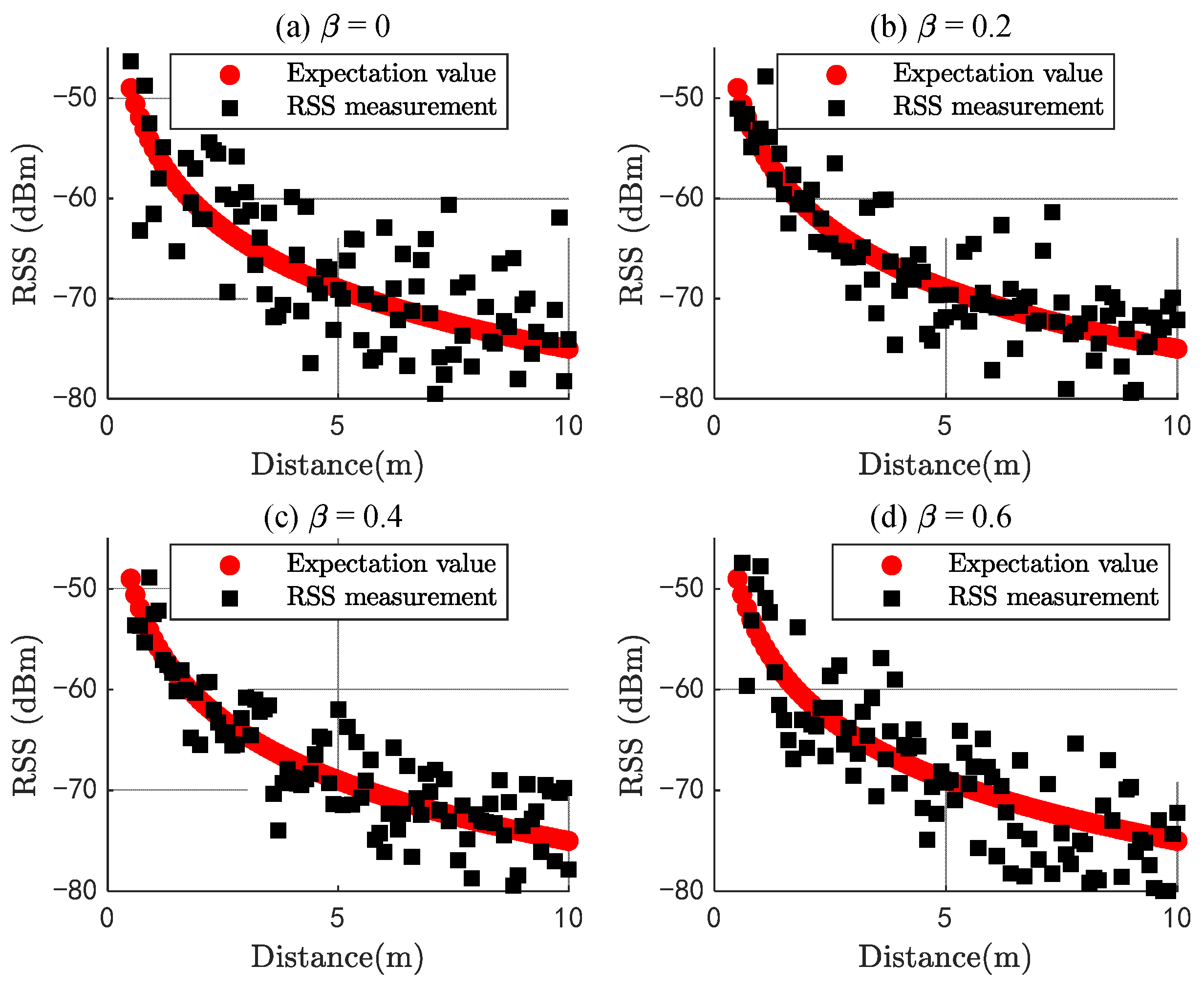
2.5. Optimal Configuration under Outliers

In this section, theoretical analysis of optimal trajectory for ASV to optimally locate a target is illustrated. Two methodologies for obtaining the optimal configuration without a target location are provided: (1) in the case of a single or two ASVs, the target position is supposed to be in an unclear zone, and (2) for the three ASVs scheme, TPLA is proposed to acquire the target location at each time slot.

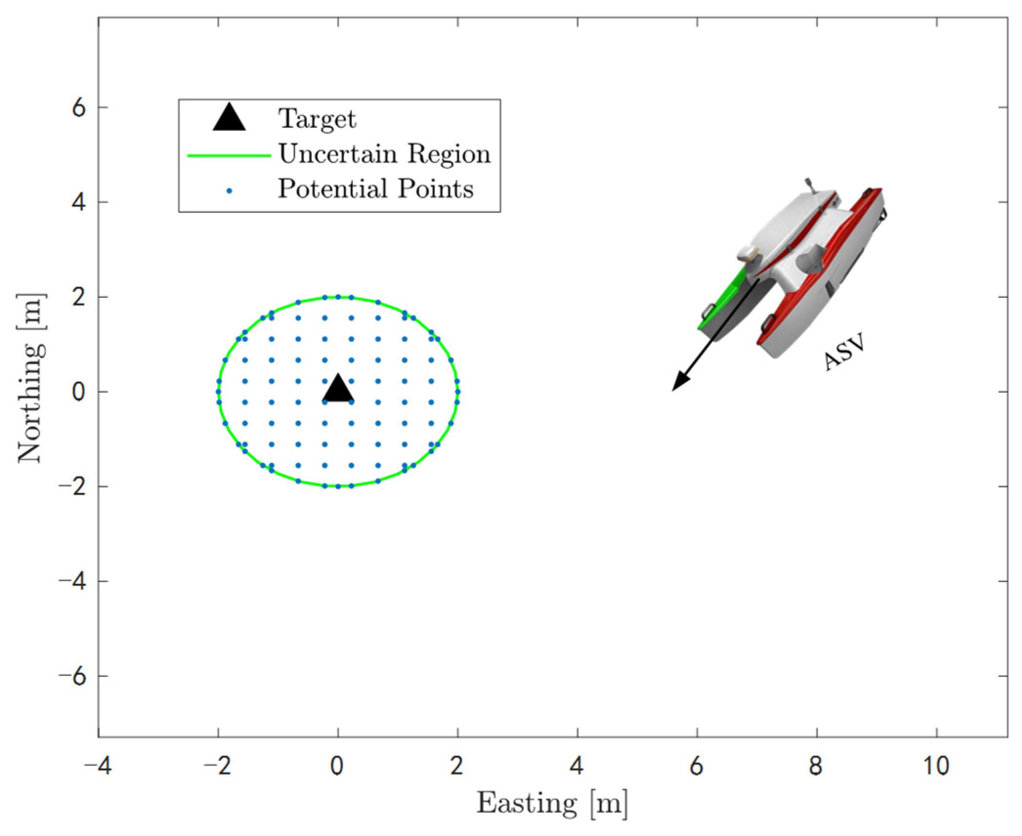
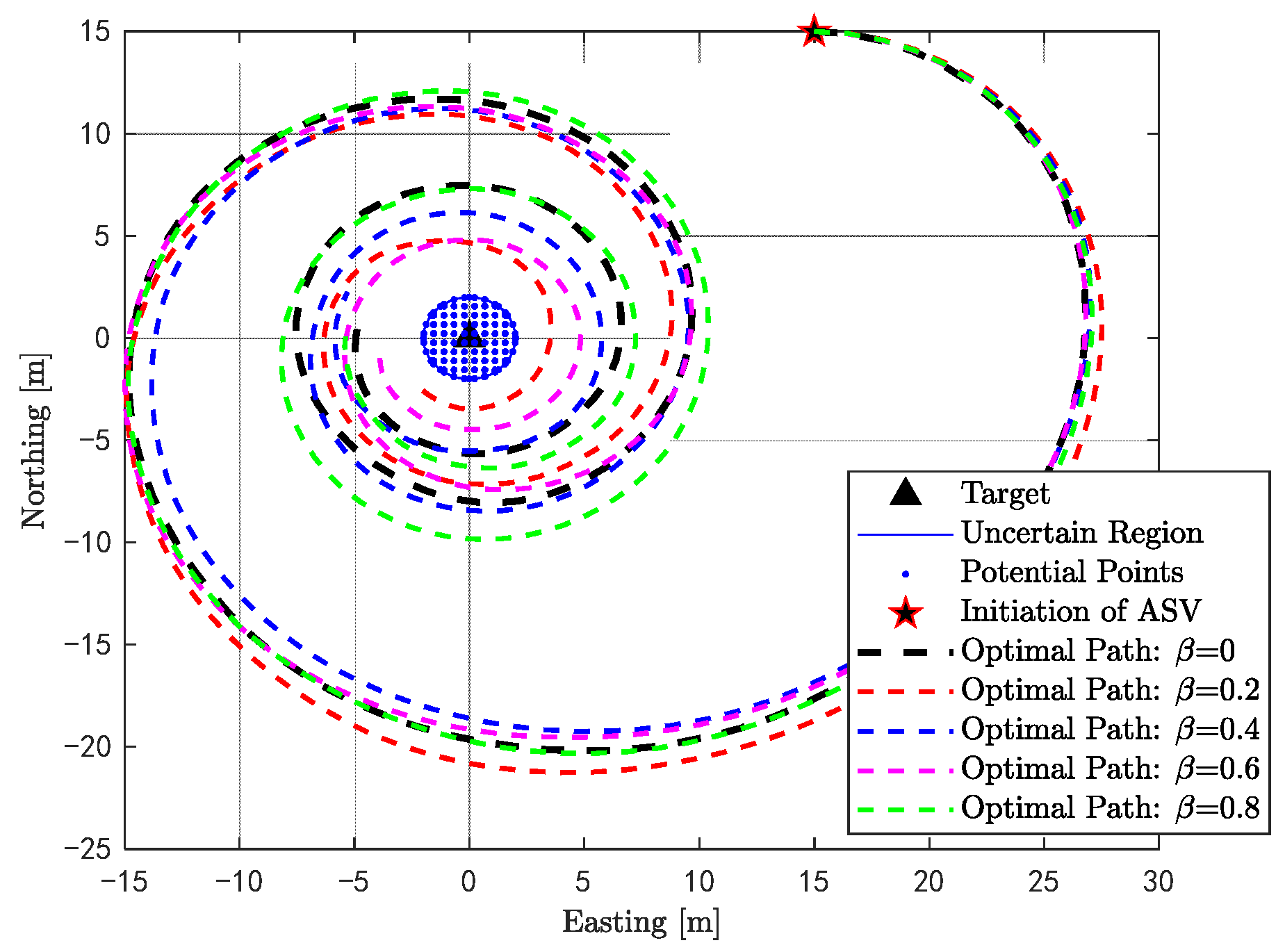
2.5.1. Optimal Trajectory for a Single ASV

It is evident from (19) that the FIM at each time slot requires knowledge of the target location. However, the true location of the target may not be known in advance especially for only one ASV involved in the mission. In this case, a min–max strategy is proposed.

Assume that the prior information of the target location is known, which drops in an uncertainty region $\Lambda$ containing several potential points, referred to as Figure 3. Suppose there are $k$ points in $\Lambda$, the problem in (19) is converted into

$$\left[\begin{array}{c}{r}_1^{*}\left(1\right)\\ ⋮\\ r_1^{*}\left(M\right)\end{array}\right]=\underset{\left|r\right|\le c, i=1}{\arg \max }{\displaystyle \sum _{t=1}^M{J}_j^t\left|{}_{j=1,\dots ,k}\right.}$$

(20)

For the sake of the maximum value of the function in (20), we should guarantee the worst situation in $\Lambda$ being maximized, i.e., maximizing the logarithm of the determinant of the FIM of a point in $\Lambda$ at time $t$ whose value is minimum.

$$\left[\begin{array}{c}{r}_1^{*}\left(1\right)\\ ⋮\\ r_1^{*}\left(M\right)\end{array}\right]=\underset{\left|r\right|\le c, i=1}{\arg \max }{\displaystyle \sum _{t=1}^M\left[\underset{j=1,\dots ,k}{\arg \min }\left(J_j^t\right)\right]}$$

(21)

Let ${\theta }^t={\left[J_1^t,\dots ,J_k^t\right]}^T$. Assume there exists a point $\wp \in k$ at time $t$ where the logarithm of the determinant of the FIM is minimum. The yaw rate at $t+1$ is determined by the yaw rate at $t$ such that the function in (22) is maximum.

$$\left[r_1^{*}\left(t\right)\right]=\underset{\left|r\right|\le c}{\arg \max }{\displaystyle {\sum }_{t-1}^t{J}_{\wp }^t}.$$

(22)

The entire process can be simply concluded as

1.

Input the initial parameters including $v\left(0\right)$, ${\mathit{A}}_1^0$, ${\phi }_1\left(0\right)$, $r_1\left(0\right)$, and potential points in the uncertain area.

2.

Figure out ${\left(I_{\eta }\right)}^t$ according to (16) at each time slot.

3.

Find the point $\wp$ to make the logarithm of the determinant of the FIM minimum.

4.

Calculate $r_1^{*}\left(t\right)$ according to (22) with the point $\wp$.

5.

Calculate ${\varphi }_1\left(t\right)$ according to ${\varphi }_1\left(t-1\right)$ and $r_1^{*}\left(t\right)$.

6.

Compute ${\mathit{A}}_1^t$ using (3) with ${\mathit{A}}_1^{t-1}$.

7.

Output ${\mathit{A}}_1^t$.

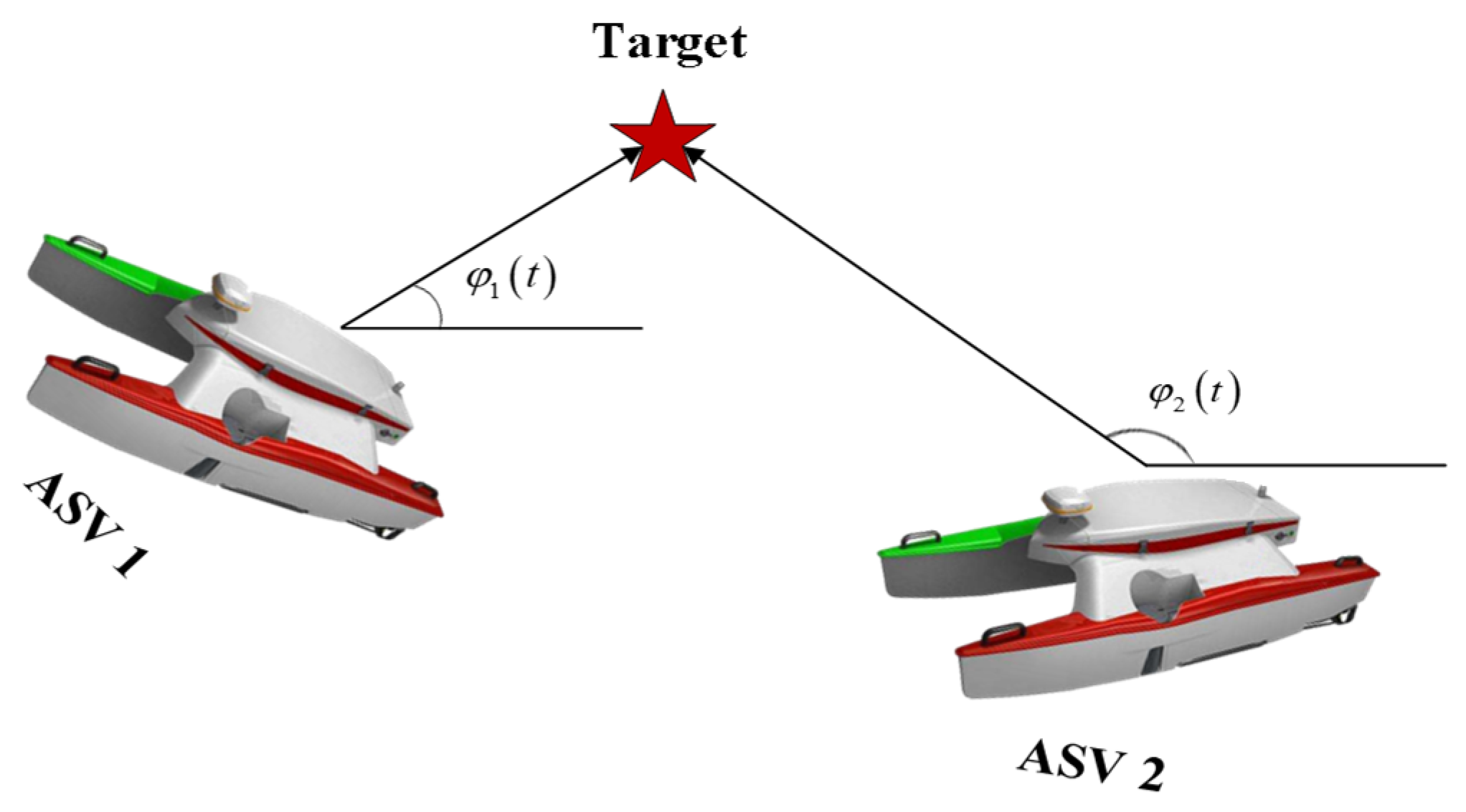
2.5.2. Optimal Trajectories for Two ASVs

When it comes to two ASVs, apparently, the position of the target at each time slot still cannot be determined by the multilateration techniques. The min–max strategy proposed in the previous section would be used in the two ASVs scenario as well. Consequently, the optimization problem of (19) goes to

$$\left[\begin{array}{cc}{r}_1^{*}\left(1\right)& r_2^{*}\left(1\right)\\ ⋮& ⋮\\ r_1^{*}\left(M\right)& r_2^{*}\left(M\right)\end{array}\right]=\underset{\left|r\right|\le c}{\arg \max }{\displaystyle \sum _{i=1}^2{\displaystyle \sum _{t=1}^M\left[\underset{j=1,\dots ,k}{\arg \min }\left(J_j^t\right)\right]}}$$

(23)

Nevertheless, the initial displacement of two ASVs then comes out, which is supposed to be the initial geometry of the ASVs. Let ${\phi }_i\left(t\right)$ denote the angle between the $i$th ASV and the target, as shown in Figure 4.

Proposition 1.

Let ${\alpha }_{12}$ be the angle between ASV 1 and ASV 2, without loss of generality, ${\alpha }_{12}={\alpha }_{21}$. For the arbitrarily fixed $‖{\mathit{B}}^t-{\mathit{A}}_i^t‖$, the determinant of FIM is maximized when ${\alpha }_{12}={\alpha }_{21}=\pi /2$.

Proof. 

Let ${\gamma }_i={\tau /‖{\mathit{B}}^t-{\mathit{A}}_i^t‖}^2$, where $\tau ={\left(I_{\eta }\right)}^t\cdot {\vartheta }^2$, and with no loss of generality let ${\gamma }_2=\zeta {\gamma }_1$ for some constant $\gamma >0$. At each time slot, the objective could be expressed as

$$J^t=J_1^t+J_2^t=\frac{\Xi }{4}\left[{\left({\displaystyle \sum _{i=1}^2\frac{1}{{‖{\mathit{B}}^t-{\mathit{A}}_i^t‖}^2}}\right)}^2-{\left({\displaystyle \sum _{i=1}^2\frac{\cos \left(2{\phi }_i\left(t\right)\right)}{{‖{\mathit{B}}^t-{\mathit{A}}_i^t‖}^2}}\right)}^2-{\left({\displaystyle \sum _{i=1}^2\frac{\sin \left(2{\phi }_i\left(t\right)\right)}{{‖{\mathit{B}}^t-{\mathit{A}}_i^t‖}^2}}\right)}^2\right].$$

(24)

The maximization of the logarithm of the determinant of (24) is equivalent to the minimization of (25) [33].

$${\left({\displaystyle \sum _{i=1}^2\frac{\cos \left(2{\phi }_i\left(t\right)\right)}{{‖{\mathit{B}}^t-{\mathit{A}}_i^t‖}^2}}\right)}^2+{\left({\displaystyle \sum _{i=1}^2\frac{\sin \left(2{\phi }_i\left(t\right)\right)}{{‖{\mathit{B}}^t-{\mathit{A}}_i^t‖}^2}}\right)}^2.$$

(25)

Then, we have

$$\begin{array}{l}{\gamma }_1^2\left[\sin \left(2{\phi }_1\left(t\right)\right)+\zeta \sin {\left(2{\phi }_2\left(t\right)\right)}^2+\left(\cos \left(2{\phi }_1\left(t\right)\right)+\zeta \cos {\left(2{\phi }_2\left(t\right)\right)}^2\right)\right]\\ ={\gamma }_1^2\left[1+\zeta +\zeta \cos \left(2{\phi }_1\left(t\right)-2{\phi }_2\left(t\right)\right)\right].\end{array}$$

Obviously, the minimum of (24) could be obtained when $\cos \left(2{\phi }_1\left(t\right)-2{\phi }_2\left(t\right)\right)=-1$. Thus, ${\phi }_2\left(t\right)-{\phi }_1\left(t\right)=ƛ\pi -\pi /2$ for $ƛ\in \mathbb{N}$ and the angle at the target by the ASVs is ${\alpha }_{12}={\alpha }_{21}={\phi }_2\left(t\right)-{\phi }_1\left(t\right)\mathrm{mod}\left(\pi \right)=\pi /2$. □

However, because the exact location of the target is unknown, the initial geometry of two ASVs is supposed to closely approximate $\pi /2$. The entire process is similar to the single ASV scenario except the initial geometry of two ASVs should be preset.

2.5.3. Optimal Trajectories for Three ASVs

As for the number of ASVs is equal to or more than three, the multilateration technique can be used to determine the target location at each time slot [40]. In this part, a novel localization method, i.e., TPLA, is proposed to locate the target and the initial geometry of three ASVs is discussed.

Optimal Initial Geometry of Three ASVs

Proposition 2.

The determinant of FIM in (13) is equivalent to

$$\det \left(\mathit{F}\mathit{I}{\mathit{M}}^t\right)=\Xi \cdot {\displaystyle \sum _S\frac{{\sin }^2\left({\phi }_i\left(t\right)-{\phi }_l\left(t\right)\right)}{{‖{\mathit{B}}^t-{\mathit{A}}_i^t‖}^2{‖{\mathit{B}}^t-{\mathit{A}}_l^t‖}^2}},S=\left\{\left\{i,l\right\}\right\}.$$

(26)

Proof. 

Let $\mathit{G}={\nabla }_{{\mathit{B}}^t}{z}_i^t$ such that $FI{M}^t={\mathit{G}}^T\mathit{G}$. Using the Cauchy–Binet formula, then we have

$$\det \left(\mathit{F}\mathit{I}{\mathit{M}}^t\right)=\Xi \cdot \det \left({\mathit{G}}^T\mathit{G}\right)=\Xi \cdot {{\displaystyle \sum _{q=\left\{1,\cdots ,\left(\begin{array}{c}N\\ 2\end{array}\right)\right\}}\det \left({\mathit{G}}_q\right)}}^2,$$

(27)

where ${\mathit{G}}_q$ is a 2 × 2 minor of $\mathit{G}$ acquired from the set of minors indexed by $S=\left\{\left\{i,j\right\}\right\}$.

All 2 × 2 minors of $\mathit{G}$ are given as

$${\mathit{G}}_S=\sqrt{\Xi }\left[\begin{array}{cc}‖{\mathit{B}}^t-{\mathit{A}}_i^t‖\cos \left({\phi }_i\left(t\right)\right)& ‖{\mathit{B}}^t-{\mathit{A}}_i^t‖\sin \left({\phi }_i\left(t\right)\right)\\ ‖{\mathit{B}}^t-{\mathit{A}}_l^t‖\cos \left({\phi }_l\left(t\right)\right)& ‖{\mathit{B}}^t-{\mathit{A}}_l^t‖\sin \left({\phi }_l\left(t\right)\right)\end{array}\right].$$

(28)

where $S=\left\{\left\{i,j\right\}\right\}$ is defined as the set of all combinations of $i$ and $l$ ($i,l\in \left\{1,\cdots ,N\right\}$ and $l>i$) with $\left|S\right|=\left(\begin{array}{c}N\\ 2\end{array}\right)$. □

As for $N=3$, let ${\alpha }_{12}$, ${\alpha }_{13}$, and ${\alpha }_{23}$ be the angles among the $i$th and $l$th ASV, ${\gamma }_{il}={\gamma }_i\cdot {\gamma }_l$, where ${\gamma }_i={\tau /‖{\mathit{B}}^t-{\mathit{A}}_i^t‖}^2$ with $\tau ={\left(I_{\eta }\right)}^t\cdot {\vartheta }^2$. Without loss of generality, ${\alpha }_{12}={\alpha }_{21}$, ${\alpha }_{13}={\alpha }_{31}$, and ${\alpha }_{23}={\alpha }_{32}$.

The relationship of angles among the $i$th and $l$th ASV could be expressed as

$$\begin{array}{l}{\alpha }_{12}=\frac{1}{2}\arccos \left(\frac{{\gamma }_{13}^2{\gamma }_{23}^2-{\gamma }_{12}^2{\gamma }_{23}^2-{\gamma }_{12}^2{\gamma }_{13}^2}{2{\gamma }_{12}^2{\gamma }_{13}{\gamma }_{23}}\right),\\ {\alpha }_{13}=\frac{1}{2}\arccos \left(\frac{{\gamma }_{12}^2{\gamma }_{23}^2-{\gamma }_{12}^2{\gamma }_{13}^2-{\gamma }_{13}^2{\gamma }_{23}^2}{2{\gamma }_{12}{\gamma }_{13}^2{\gamma }_{23}}\right),\\ {\alpha }_{23}=\pi -{\alpha }_{12}-{\alpha }_{13}.\end{array}$$

(29)

If ${\gamma }_l>{\displaystyle {\sum }_{1\le i\le 3,i\ne l}{\gamma }_i}$, which means one ASV is close to the target, then

$${\phi }_r=\pm \frac{\pi }{2}+{\phi }_i,r\in \left\{1,2,3\right\}\backslash i.$$

(30)

According to [33], (30) could be further interpreted as

$$\left\{\begin{array}{ll}{\alpha }_{il}=\frac{\pi }{2},& \mathrm{if} {\gamma }_{il}>{\gamma }_{rl}, \forall rl\in \left\{12,13,23\right\}\backslash \left\{il\right\}\\ {\alpha }_{il}=0 \mathrm{or} \pi ,& \mathrm{otherwise}\end{array}\right.,$$

(31)

where $\backslash$ is the set subtraction.

However, when ${\gamma }_1={\gamma }_2={\gamma }_3$, there exists a particular solution, i.e., ${\alpha }_{12}={\alpha }_{12}={\alpha }_{23}=2\pi /3$ or ${\alpha }_{12}={\alpha }_{23}=\pi /3$ and ${\alpha }_{13}=2\pi /3$.

It should be noted that the initial geometry of multiple ASVs (more than 3) is highly related to that of two or three ASVs [33,56]. ASVs could be clustered into smaller groups with two or three ASVs. Then, the optimal geometry would be obtained by optimizing the angle in each group, which is not considered in this paper.

TPLA

To determine the target location at each time slot, a simple manipulation is conducted from (4) when $d_0=1 \mathrm{m}$ [57], as given by

$$‖{\mathit{B}}^t-{\mathit{A}}_i^t‖\approx {10}^{\frac{P_0-z_i^t}{10\vartheta }}\cdot {10}^{\frac{\eta }{10\vartheta }}.$$

(32)

The right side of (32) can be approximated using the first-order Taylor series expansion as [58]

$${\lambda }_i^t‖{\mathit{B}}^t-{\mathit{A}}_i^t‖\approx \hslash \left(1+\frac{\ln 10}{10\vartheta }\eta \right),$$

(33)

where ${\lambda }_i^t={10}^{\frac{z_i^t}{10\vartheta }}$ and $\hslash ={10}^{\frac{P_0}{10\vartheta }}$.

Then, the localization problem can be formulated as

$$\underset{{\mathit{B}}^t}{{\displaystyle \arg \min }}{\displaystyle \sum _{i=1}^N{\left(‖{\mathit{B}}^t-{\mathit{A}}_i^t‖-\frac{\hslash }{{\lambda }_i^t}\right)}^2}.$$

(34)

After squaring each term and proper manipulation, the considered problem is then converted into a non-linear least-square form as

$$\underset{{\mathit{B}}^t}{\arg \min }{\displaystyle \sum _{i=1}^N{\omega }_i{\left({\left({\lambda }_i^t\right)}^2{‖{\mathit{B}}^t-{\mathit{A}}_i^t‖}^2-{\hslash }^2\right)}^2},$$

(35)

where ${\omega }_i$ denotes the weight that could be expressed as ${\omega }_i=1-{\widehat{d}}_i^t/\left({\displaystyle {\sum }_{i=1}^N{\widehat{d}}_i^t}\right)$, and ${\widehat{d}}_i^t$ is the approximated distance between the $i$th ASV and the target.

The problem is further converted into a generalized trust region subproblem (GTRS) through expanding the squared norm in (35), as given by

$$\begin{array}{l}\underset{y}{J\left(\mathit{y}\right)=\mathrm{minimize}} {‖\mathit{\omega }(\mathit{\Im }\mathit{y}-\mathit{\kappa })‖}^2,\\ \mathrm{subject} \mathrm{to} {\mathit{y}}^T\mathit{D}\mathit{y}+2{\mathit{l}}^T\mathit{y}=0,\end{array}$$

(36)

where $\mathit{y}={[{\left({\mathit{B}}^t\right)}^T,{‖{\mathit{B}}^t‖}^2]}^T$, $\mathit{\omega }=diag\left(\left[{\omega }_1{}^2,\dots ,{\omega }_N{}^2\right]\right)$, $\mathit{D}=diag\left(\left[1,1,0\right]\right)$, $\mathit{l}={\left[0,0,-0.5\right]}^T$, and

$$\mathit{\Im }=\left[\begin{array}{cc}\begin{array}{l}2{\left({\lambda }_1^t\right)}^2{a}_1^T\\ ⋮\\ 2{\left({\lambda }_N^t\right)}^2{a}_N^T\end{array}& \begin{array}{l}-{\left({\lambda }_1^t\right)}^2\\ ⋮\\ -{\left({\lambda }_N^t\right)}^2\end{array}\end{array}\right],\mathit{\kappa }=\left[\begin{array}{l}\left({\left({\lambda }_1^t\right)}^2{‖a_1‖}^2-{\hslash }^2\right)\\ ⋮\\ \left({\left({\lambda }_N^t\right)}^2{‖a_N‖}^2-{\hslash }^2\right)\end{array}\right].$$

The problem in (36) could be solved using a bisection method [59]. However, we cannot ensure that the multiplier interval is strictly decreasing during the iteration in the bisection method, which may degrade the localization accuracy. In this case, a majorization minimization form is constructed, where the solution from the bisection method initiates the iteration.

Recall the problem in (34), a surrogate function is acquired by dropping the constant term as

$$S\left({\mathit{B}}^t\right)=\underset{f\left(x\right)}{\underbrace{{\displaystyle \sum _{i=1}^N{‖{\mathit{B}}^t-{\mathit{A}}_i^t‖}^2}}}+\underset{g\left(x\right)}{\underbrace{\left[-2{\displaystyle \sum _{i=1}^N\left(\frac{\hslash }{{\lambda }_i^t}‖{\mathit{B}}^t-{\mathit{A}}_i^t‖\right)}\right]}},$$

(37)

where, apparently, $f\left(x\right)$ is convex and $g\left(x\right)$ is concave.

Theoretically, the concave term would be upper bounded at ${\left({\mathit{B}}^t\right)}^Z$ via first-order Taylor expansion [60], wherein $Z$ is the iteration, such that

$$g({\mathit{B}}^t)\le g\left({\left({\mathit{B}}^t\right)}^Z\right)+\nabla g{\left({\left({\mathit{B}}^t\right)}^Z\right)}^T\left({\mathit{B}}^t-{\left({\mathit{B}}^t\right)}^Z\right).$$

(38)

After maximizing $g\left(x\right)$, then we have

$$S\left({\mathit{B}}^t\left|{\left({\mathit{B}}^t\right)}^Z\right.\right)={\displaystyle \sum _{i=1}^N\left({‖{\mathit{B}}^t-{\mathit{A}}_i^t‖}^2-2\cdot \frac{\hslash }{{\lambda }_i^t}‖{\mathit{B}}^t-{\mathit{A}}_i^t‖\right)}-2{\displaystyle \sum _{i=1}^M\frac{\hslash }{{\lambda }_i^t}\frac{{\left({\left({\mathit{B}}^t\right)}^Z-{\mathit{A}}_i^t\right)}^T}{‖{\left({\mathit{B}}^t\right)}^Z-{\mathit{A}}_i^t‖}\left({\mathit{B}}^t-{\left({\mathit{B}}^t\right)}^Z\right)}.$$

(39)

The update rule for $x^{Z+1}$ could be expressed as

$${\left({\mathit{B}}^t\right)}^{Z+1}=\frac{1}{N}{\displaystyle \sum _{i=1}^N\left({\mathit{A}}_i^t+\frac{\hslash }{{\lambda }_i^t}\frac{{\left({\left({\mathit{B}}^t\right)}^Z-{\mathit{A}}_i^t\right)}^T}{‖{\left({\mathit{B}}^t\right)}^Z-{\mathit{A}}_i^t‖}\right)}.$$

(40)

The entire localization process could be concluded in Algorithm 1.

Algorithm 1. TPLA

1. Input: $y_{\mathrm{prev}}=0$, $threshold=1e-7$, $iter=1$, total number of iterations at the first phase     $I_1$, and the second phase $I_2$.

2. Calculate the RSS measurements

3. Reshape the problem to a GTRS problem as (35).

4. While $iter<I_1$ do

5.    Determine the multiplier λ at each iteration according to

${\left(\frac{{\mathit{\Im }}^T{\mathit{\omega }}^T\mathit{\kappa }-ƛ\mathit{l}}{{\mathit{\Im }}^T\mathit{\omega }\mathit{\Im }+ƛ\mathit{D}}\right)}^T\mathit{D}\left(\frac{{\mathit{\Im }}^T{\mathit{\omega }}^T\mathit{\kappa }-ƛ\mathit{l}}{{\mathit{\Im }}^T\mathit{\omega }\mathit{\Im }+ƛ\mathit{D}}\right)+2f^T\left(\frac{{\mathit{\Im }}^T{\mathit{\omega }}^T\mathit{\kappa }-ƛ\mathit{l}}{{\mathit{\Im }}^T\mathit{\omega }\mathit{\Im }+ƛ\mathit{D}}\right)=0$

6.     ${\mathsf{ƛ}}^{\mathrm{iter}*}=\max \left[-diag\left({\mathit{\Im }}^T\mathit{\omega }\mathit{\Im }\right)/diag\left(\mathit{D}\right), ƛ\right]$

7.    Determine the optimal $\mathit{y}$ at each iteration according to ${\mathit{y}}^{iter}=\frac{{\mathit{\Im }}^T{\mathit{\omega }}^T\mathit{\kappa }-{ƛ}^{k*}\mathit{l}}{{\mathit{\Im }}^T\mathit{\omega }\mathit{\Im }+{ƛ}^{k*}\mathit{D}}$

8.     If $‖{\mathit{y}}^{iter}-{\mathit{y}}_{prev}‖/‖{\mathit{y}}^{iter}‖<threshold$

9.         Break

10.    End if

11.    ${\mathit{y}}_{prev}={\mathit{y}}^{iter}$

12. End while

13. Output ${\mathit{B}}^t$ (as the input to the second phase)

14. ${\left({\mathit{B}}^t\right)}^1\leftarrow {\mathit{B}}^t$$, \mathrm{and} Z\leftarrow 1$

15. While $\left(Z<I_2\right)$ do

16.      Update ${\left({\mathit{B}}^t\right)}^{Z+1}$ according to (40)

17. End while

18. Output: ${\mathit{B}}^t\leftarrow {\left({\mathit{B}}^t\right)}^I$

Convergence Analysis of TPLA

TPLA consists of two steps: (1) the GTRS step solved by a bisection method and (2) Taylor linearization approximation by an iteration method. The output of GTRS is considered as the input for the second step, as reference to Algorithm 1. In this case, the proof of convergence for TPLA is equivalent to that of the second step.

Proposition 3.

Given any${\mathit{B}}^t={\left({\mathit{B}}^t\right)}^Z$, $-‖{\mathit{B}}^t-{\mathit{A}}_i^t‖$ is upper bounded as

$$-‖{\mathit{B}}^t-{\mathit{A}}_i^t‖\le -\frac{{\left({\left({\mathit{B}}^t\right)}^Z-{\mathit{A}}_i^t\right)}^T}{‖{\left({\mathit{B}}^t\right)}^Z-{\mathit{A}}_i^t‖}\left({\mathit{B}}^t-{\left({\mathit{B}}^t\right)}^Z\right).$$

(41)

Proof. 

By employing the Cauchy–Schwarz inequality, we have

$${\left({\left({\mathit{B}}^t\right)}^Z-{\mathit{A}}_i^t\right)}^T\left({\mathit{B}}^t-{\left({\mathit{B}}^t\right)}^Z\right)\le ‖{\mathit{B}}^t-{\mathit{A}}_i^t‖‖{\left({\mathit{B}}^t\right)}^Z-{\mathit{A}}_i^t‖.$$

(42)

By rearranging the term and taking the negative sign in (42), the inequality of (41) can be proved. □

Proposition 4.

Given a sequence of $\left\{{\left({\mathit{B}}^t\right)}^Z\right\}$, the objective of (37) is non-increasing and converges to a stationary point.

Proof. 

Subject to (38), we have

$$S\left({\mathit{B}}^t\left|{\left({\mathit{B}}^t\right)}^Z\right.\right)-S\left({\mathit{B}}^t\right)=g\left({\left({\mathit{B}}^t\right)}^Z\right)-g\left({\mathit{B}}^t\right)+\nabla g{\left({\left({\mathit{B}}^t\right)}^Z\right)}^T\left({\mathit{B}}^t-{\left({\mathit{B}}^t\right)}^Z\right).$$

(43)

Integrated with Proposition 3, then the function can be upper bounded as

$$S\left({\mathit{B}}^t\left|{\left({\mathit{B}}^t\right)}^Z\right.\right)-S\left({\mathit{B}}^t\right)\ge S\left({\left({\mathit{B}}^t\right)}^Z\left|{\left({\mathit{B}}^t\right)}^Z\right.\right)-S\left({\left({\mathit{B}}^t\right)}^Z\right).$$

(44)

Apparently, $S\left({\mathit{B}}^t\left|{\left({\mathit{B}}^t\right)}^Z\right.\right)-S\left({\mathit{B}}^t\right)$ is convex since an affine function and a convex term are included. With the derivative of ${\mathit{B}}^t$, then we have

$$\begin{array}{l}S\left({\left({\mathit{B}}^t\right)}^{Z+1}\right)\le S\left({\left({\mathit{B}}^t\right)}^{Z+1}\left|{\left({\mathit{B}}^t\right)}^Z\right.\right)-S\left({\left({\mathit{B}}^t\right)}^Z\left|{\left({\mathit{B}}^t\right)}^Z\right.\right)+S\left({\left({\mathit{B}}^t\right)}^Z\right)\le \\ S\left({\left({\mathit{B}}^t\right)}^Z\left|{\left({\mathit{B}}^t\right)}^Z\right.\right)-S\left({\left({\mathit{B}}^t\right)}^Z\left|{\left({\mathit{B}}^t\right)}^Z\right.\right)+S\left({\left({\mathit{B}}^t\right)}^Z\right)=S^{*}.\end{array}$$

(45)

Therefore, the objective of (37) is non-increasing and converges to a stationary point. □

According to Propositions 3 and 4, the convergence of TPLA can be proved.

Optimal Trajectories of Three ASVs

Generally, the initial geometry of three ASVs is preset according to the reduction. Afterwards, the optimal yaw rate of the ASVs would be acquired via solving (19) after determining the target location using TPLA at each time slot. The optimal waypoint of each ASV at time $t+1$ is determined using the point at time $t$, directly solved using the Matlab optimization tool box [55]. The whole process is repeated until the geolocation mission is completed.

3. Results and Discussion

In this section, we perform simulations in Matlab R2018b under various scenarios to demonstrate the propositions and the proposed method for obtaining the optimal trajectory under outliers. The situation with a single ASV is presented first, followed by scenarios with two and three ASVs.

3.1. Parameters Setup

To verify the analytical findings of the optimal trajectory of ASVs for localization, we conduct the simulations, wherein the corresponding parameters are set below: $P_0=-55 \mathrm{dBm}$, $\vartheta =3$, ${\sigma }^2=2 \mathrm{dB}$, and $I_1=I_2=100$. The outlier type in the simulations is considered to yield a uniform distribution following $\left[-\sqrt{2},\sqrt{2}\right]$ [4,61]. The maximum Monte Carlo simulation is 1000, where $N_C=1000$. The yaw rate follows $r\in \left[-{20}^{°},{20}^{°}\right] \mathrm{rad}/\mathrm{s}$ [13]. In the simulation, we set $t=1$ as the start period time. We use an interior point method in the toolbox of Matlab R2018b to solve the optimization problem in (19) due to the simplicity and fast speed for the convergence [62]. The velocity, initial heading, and yaw rate of the ASVs are different in each scenario, described in the following parts.

3.2. Optimal Trajectory of a Single ASV

First, we conduct a simulation of the optimal trajectory of a single ASV with the static target, where $\beta$ varies from 0 to 0.8 to determine how the outliers influence the trajectory. The radius of the uncertain region is 2 m and the speed of the ASV is 1.5 m/s. In addition, the rest of parameters for the scenario are set up with ${\mathit{A}}_1^1={\left[15,15\right]}^T$, $\mathit{B}={\left[0,0\right]}^T$, ${\varphi }_1\left(1\right)=\pi /2$, $r_1\left(1\right)=0 \mathrm{rad}/\mathrm{s}$, $M=200$, and $k=96$.

The optimal trajectories of a single ASV and their yaw rate under variable $\beta$ are shown in Figure 5 and Figure 6, where $\beta =0$ means no outliers are involved in the measurements. It can be seen from Figure 5 that the optimal trajectories are more like a circle and the radius of the circle becomes smaller. In addition, interestingly, the trajectories with outliers seem closer to that without outliers. This is because (1) for $N$ spatially disparate sensors, the optimal placement for sensors is uniformly distributed along any circle around the target according to Corollary 1, and (2) for RSS-based localization, the closer to the target, the more valuable accurate range information would be provided because of log-normal shadowing in (4). Thus, for the optimal trajectories, it can be argued that the ASV must move circularly around and closer to the target, referred to as Figure 5.

One more interesting thing that is worth noting is that with the uniform distributed outliers involved in the measurement model (4), the value of the objective is becoming larger, referred to as Figure 7, which is equivalent to the increase in the determinant of FIM. The larger the determinant of FIM, the smaller the CRLB that would be obtained according to (8). Accordingly, the trajectories with the uniform distributed outliers become closer to the target, and the radius for the circle seems less than that without outliers. In addition to the static target, we simulate a scenario with a dynamic target. According to Remark 5 in [13], the target speed should be much lower than that of the ASV; otherwise, no feasible solution would be acquired. Therefore, the speed of the target we set in the simulation is $v_x=v_y=0.1 \mathrm{m}/\mathrm{s}$ and the time step is $M=150 \mathrm{s}$. Due to the discussion of the influence of the variable $\beta$ on the optimal trajectories, we only carry out the simulation with $\beta =0, \mathrm{and} 0.8$ in terms of the optimal trajectory. As expected, from Figure 8, the ASV moves circularly and becomes closer to the target in the scenario of the static target. The difference between the dynamic scenario and the static scenario is that the circle would be movable along with the moving target.

3.3. Optimal Trajectories of Two ASVs

In this part, we first conduct the scenario of the optimal trajectories with a static target and then expand the scenario with a dynamic target. The radius of the uncertain region is 2 m and the speed of the ASV1 and ASV2 is 1.5 m/s. The rest of parameters are set as ${\mathit{A}}_1^1={\left[30,30\right]}^T$, ${\mathit{A}}_2^1={\left[30,-30\right]}^T$, $\mathit{B}={\left[0,0\right]}^T$, ${\varphi }_1\left(1\right)=\pi /2$, ${\varphi }_2\left(1\right)=0$, $r_1\left(1\right)=\pi /30 \mathrm{rad}/\mathrm{s}$, $r_2\left(1\right)=\pi /18 \mathrm{rad}/\mathrm{s}$, $M=400$, $\beta =0.4$, and $k=96$.

Following Proposition 1, the optimal geometry for two ASVs in the simulation is $\pi /2$. Here, trajectories with $\beta =0.4$ are only discussed in the scenario with two ASVs because the full discussion of the influence of variable $\beta$ on optimal trajectories was considered in the scenario with a single ASV. It can be seen from Figure 9 that two ASVs move circularly and close to the target until reaching the minimum radius.

The scenario with a dynamic target is depicted in Figure 10, where the target speed is $v_x=0,v_y=0.3 \mathrm{m}/\mathrm{s}$. As shown in Figure 10, two ASVs move circularly and close to the moving target. The radii of circles are becoming smaller along with the moving target until a minimum is achieved.

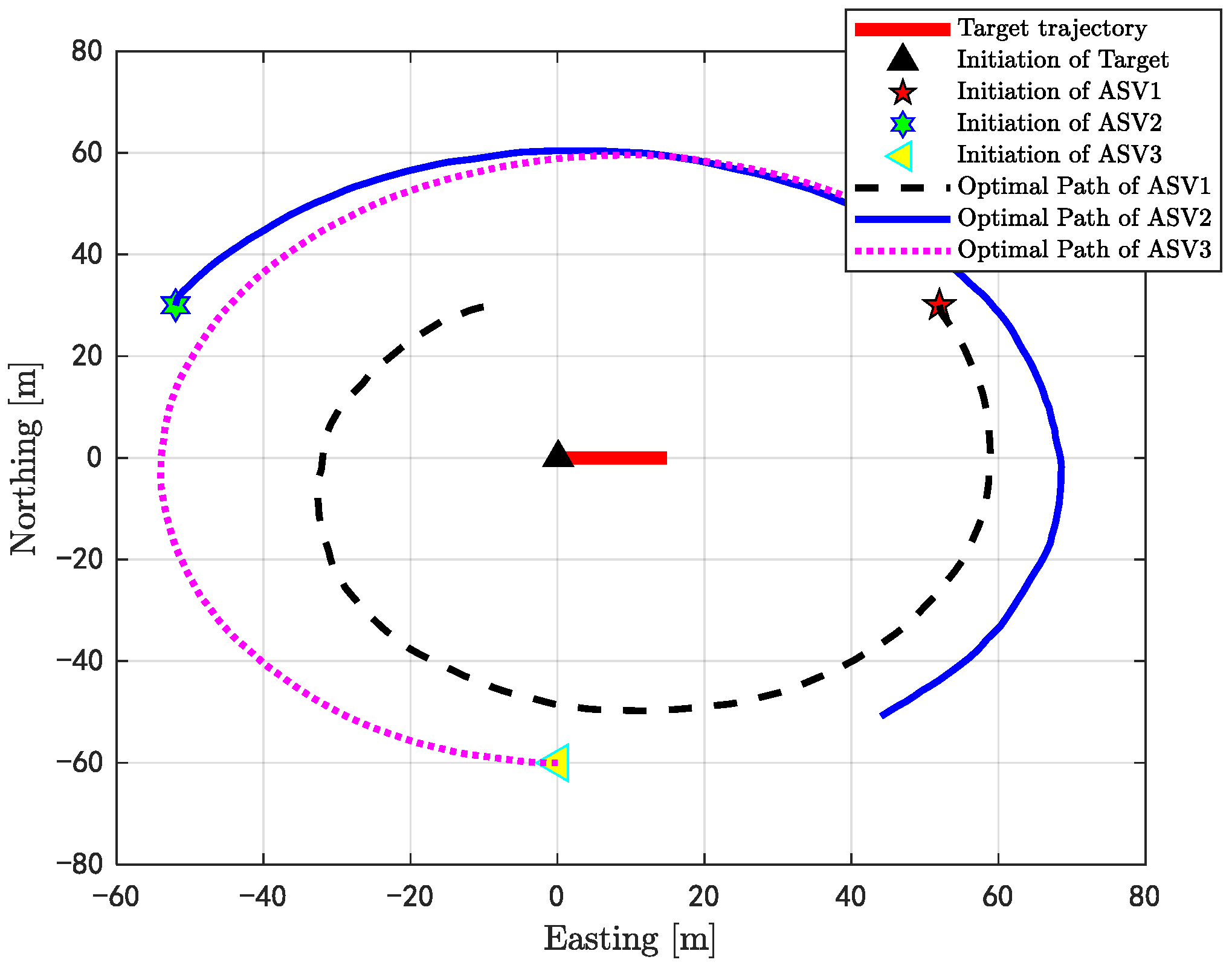
3.4. Optimal Trajectories of Three ASVs

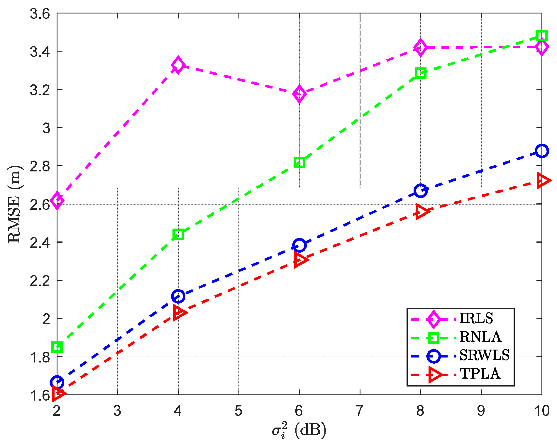
3.4.1. Localization Method Comparison

To verify the effectiveness of TPLA, a comparison is conducted with several state-of-the-art methods proposed to tackle the outliers, i.e., iterative re-weighted least squares (IRLS) [63], robust non-cooperative localization algorithm (RNLA) [4], and squared range weighted least squares (SRWLS) [57]. Due to the dynamics of the ASVs and the target, the position of the target and the ASVs are set to be changeable in a 30 × 30 m area at each Monte Carlo trial. Moreover, the root mean square error (RMSE) is conducted as the calibration, as given by

$$RMSE=\sqrt{\frac{1}{{\Gamma }_{\max }}{\displaystyle \sum _{\Gamma =1}^{{\Gamma }_{\max }}{\left(\widehat{\mathit{B}}-\mathit{B}\right)}^2}}$$

(46)

where ${\Gamma }_{\max }$ is the total number of Monte Carlo trials, $\widehat{\mathit{B}}$ is the estimate, and $\Gamma$ is the current trial.

As shown in Figure 11, the localization accuracy of all methods degrades over the rise in $\beta$. IRLS, RNLA, and SRWLS are the methods used to construct the localization problem into a GTRS, which is solved using a bisection method. The difference is the determination of the weight. IRLS and RNLA determine the weight via iteration, which is changeable, whereas SRWLS defines the weight using range information. However, it should be noted that the bisection method may have a rough approximation if the interval of the multiplier for GTRS is inappropriate. It is necessary to determine an interval of the starting point and ensure that the interval of the multiplier is strictly decreasing during the iteration. In this case, the second phase of the localization is executed in TPLA. From Figure 11, we can see intuitively that the performance of TPLA is better than others. The outperformance of TPLA can be referred to in Figure 12 as well, where the scenario of variable variances is simulated. The localization error of the methods increases over the rise in variance, among which the proposed algorithm, i.e., TPLA, enables more satisfactory results compared with others.

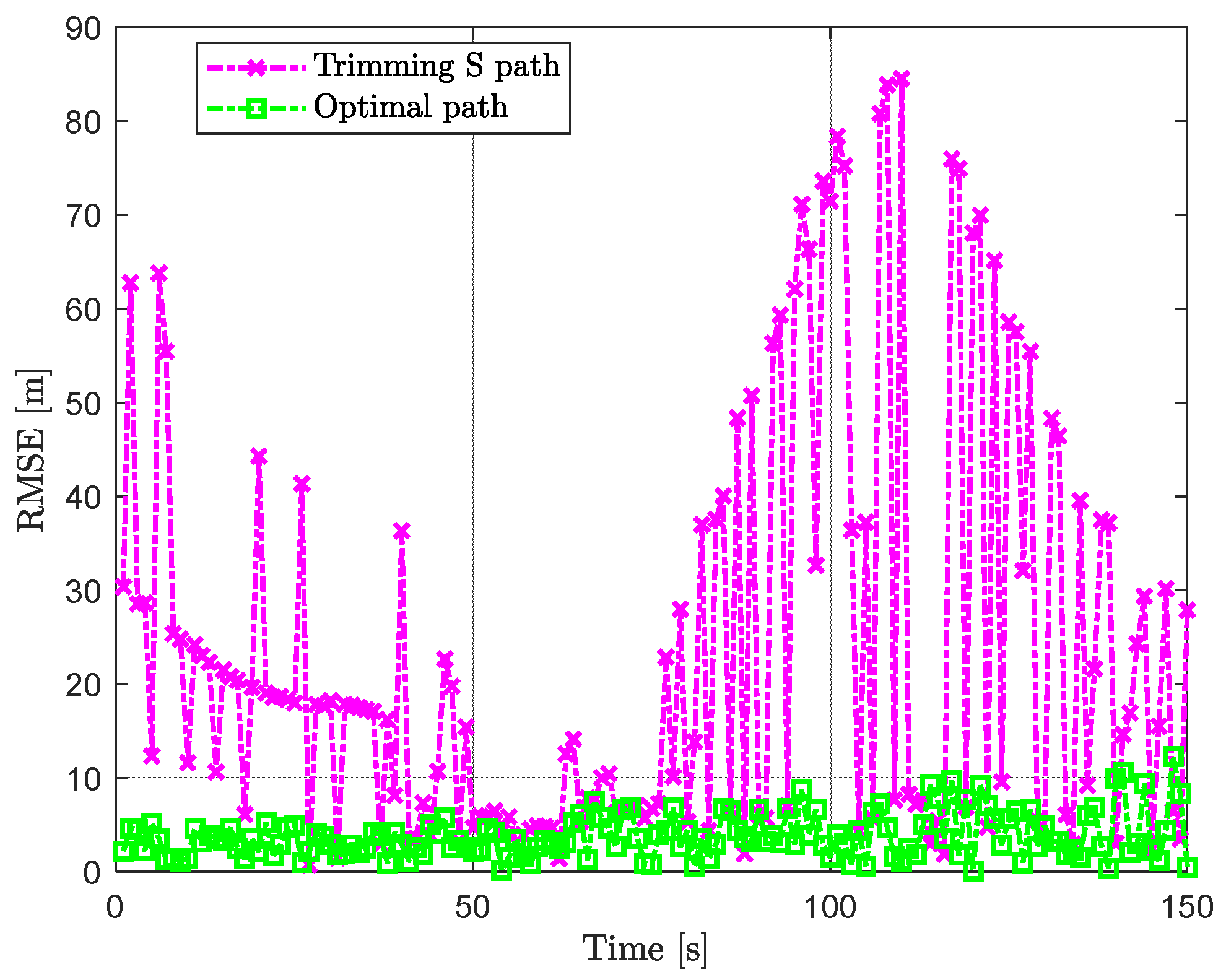
3.4.2. Optimal Trajectories

In this part, a specific scenario of optimal trajectories for three ASVs, i.e., the initial distance between ASVs and the target, is the same, and the geometry of ASVs is ${\alpha }_{12}={\alpha }_{12}={\alpha }_{23}=2\pi /3$, with a dynamic target under $\beta =0.4$ considered. The corresponding parameters are set as ${\mathit{A}}_1^1={\left[30\sqrt{3},30\right]}^T$, ${\mathit{A}}_2^1={\left[-30\sqrt{3},30\right]}^T$, ${\mathit{A}}_3^1={\left[0,-60\right]}^T$, ${\mathit{B}}^1={\left[0,0\right]}^T$, ${\varphi }_1\left(1\right)=\pi$, ${\varphi }_2\left(1\right)=0$, ${\varphi }_3\left(1\right)=-\pi /2$, $r_1\left(1\right)=\pi /18 \mathrm{rad}/\mathrm{s}$, $r_2\left(1\right)=\pi /30 \mathrm{rad}/\mathrm{s}$, $r_3\left(1\right)=\pi /10 \mathrm{rad}/\mathrm{s}$, $M=150$, $v_1=v_2=v_3=1.5 \mathrm{m}/\mathrm{s}$, $v_x=0.1 \mathrm{m}/\mathrm{s}$, $v_y=0 \mathrm{m}/\mathrm{s}$, and $\beta =0.4$.

To demonstrate further that the trajectories that we addressed are optimal, as shown in Figure 13, we carry out the simulations with the trimming trajectories mentioned in [64], referred to as Figure 14. At each time slot, the target location is determined using TPLA via the contaminated RSS measurements. It can be seen from Figure 15 that the RMSE of optimal trajectories is better than that of trimming trajectories, where the average RMSEs of the optimal trajectories and the trimming trajectories are $3.77 \mathrm{m}$ and $22.95 \mathrm{m}$, respectively.

4. Conclusions

In this paper, we developed optimal trajectories of ASVs for localization using RSS under outliers. The D-optimality integrated with a Monte Carlo strategy was presented to obtain the close-form expression of FIM. To further acquire the optimization configuration in the absence of target location, two strategies were then studied. In what concerns a single ASV or two ASVs, a min–max strategy with the imperfect knowledge of the target was proposed. As for the scenario of three ASVs, a novel localization method, i.e., TPLA, was presented to obtain the target location at each time slot. The influence of outliers on the optimal trajectories was investigated and discussed in the simulations. Moreover, a comparison between the obtained trajectories and the trimming trajectories was executed to illustrate that the analytical finding that we addressed was optimal. However, the maximum number of ASVs that the paper considered was three for convenience. Currently, some works in [65,66] have proved that when there are more than three ASVs, the optimal geometry seems be obtained by optimizing the angle in each group. Unfortunately, the scenario of multiple ASVs, generally more than three, is not addressed in the paper, which would be our future research direction. Further, collision avoidance must be considered in future research pertaining to ideal trajectories of multiple ASVs for target localization. Meanwhile, the optimal trajectory presented in the research does not account for the economic property (jointly shortest and smoothest goals). How to strike a balance between localization accuracy and economics is a topic for future research. In addition, ocean currents, particularly time-varying currents, may have a negative effect on the kinematic model, resulting in an anticipated motion when using the proposed technique. Controlling ASVs in a manner that maintains localization precision and an optimum trajectory approach with security concerns [67,68,69] is another potential direction.

References

1. Han, G.; Long, X.; Zhu, C.; Guizani, M.; Bi, Y.; Zhang, W. An AUV Location Prediction-Based Data Collection Scheme for Underwater Wireless Sensor Networks. IEEE Trans. Veh. Technol. 2019, 68, 6037–6049. [Google Scholar] [CrossRef]
2. Zhuo, X.; Liu, M.; Wei, Y.; Yu, G.; Qu, F.; Sun, R. AUV-aided Energy-Efficient Data Collection in Underwater Acoustic Sensor Networks. IEEE Internet Things J. 2020, 7, 10010–10022. [Google Scholar] [CrossRef]
3. Jing, P.; Xu, G.; Chen, Y.; Shi, Y.; Zhan, F. The Determinants behind the Acceptance of Autonomous Vehicles: A Systematic Review. Sustainability 2020, 12, 1719. [Google Scholar] [CrossRef]
4. Mei, X.; Wu, H.; Xian, J.; Chen, B.; Zhang, H.; Liu, X. A Robust, Non-Cooperative Localization Algorithm in the Presence of Outlier Measurements in Ocean Sensor Networks. Sensors 2019, 19, 2708. [Google Scholar] [CrossRef] [PubMed]
5. Wu, H.; Mei, X.; Chen, X.; Li, J.; Wang, J.; Mohapatra, P. A novel cooperative localization algorithm using enhanced particle filter technique in maritime search and rescue wireless sensor network. ISA Trans. 2018, 78, 39–46. [Google Scholar] [CrossRef]
6. Chen, X.; Ling, J.; Wang, S.; Yang, Y.; Luo, L.; Yan, Y. Ship detection from coastal surveillance videos via an ensemble Canny-Gaussian-morphology framework. J. Navig. 2021, 74, 1252–1266. [Google Scholar] [CrossRef]
7. Bayat, M.; Crasta, N.; Aguiar, A.P.; Pascoal, A.M. Range-Based Underwater Vehicle Localization in the Presence of Unknown Ocean Currents: Theory and Experiments. IEEE Trans. Control Syst. Technol. 2016, 24, 122–139. [Google Scholar] [CrossRef]
8. Su, R.; Zhang, D.; Li, C.; Gong, Z.; Venkatesan, R.; Jiang, F. Localization and Data Collection in AUV-Aided Underwater Sensor Networks: Challenges and Opportunities. IEEE Netw. 2019, 33, 86–93. [Google Scholar] [CrossRef]
9. Ma, T.; Li, Y.; Zhao, Y.; Jiang, Y.; Cong, Z.; Zhao, Q.; Xu, S. An AUV localization and path planning algorithm for terrain-aided navigation. ISA Trans. 2020, 103, 215–227. [Google Scholar] [CrossRef]
10. Mei, X.; Han, D.; Saeed, N.; Wu, H.; Ma, T.; Xian, J. Range Difference-based Target Localization under Stratification Effect and NLOS bias in UWSNs. IEEE Wirel. Commun. Lett. 2022; early access. [Google Scholar] [CrossRef]
11. Liu, Y.; Wang, H.; Cai, L.; Shen, X.; Zhao, R. Fundamentals and Advancements of Topology Discovery in Underwater Acoustic Sensor Networks: A Review. IEEE Sens. J. 2021, 21, 21159–21174. [Google Scholar] [CrossRef]
12. Sozer, E.M.; Stojanovic, M.; Proakis, J.G. Underwater acoustic networks. IEEE J. Ocean. Eng. 2000, 25, 72–83. [Google Scholar] [CrossRef]
13. Crasta, N.; Moreno-Salinas, D.; Pascoal, A.M.; Aranda, J. Multiple autonomous surface vehicle motion planning for cooperative range-based underwater target localization. Annu. Rev. Control 2018, 46, 326–342. [Google Scholar] [CrossRef]
14. Marie, T.F.B.; Yang, B.; Han, D.; An, B. A Hybrid Model Integrating MPSE and IGNN for Events Recognition along Submarine Cables. IEEE Trans. Instrum. Meas. 2022; early access. [Google Scholar] [CrossRef]
15. Chen, P.; Han, D. Effective wind speed estimation study of the wind turbine based on deep learning. Energy 2022, 247, 123491. [Google Scholar] [CrossRef]
16. Moreno-Salinas, D.; Pascoal, A.M.; Aranda, J. Optimal Sensor Trajectories for Mobile Underwater Target Positioning with Noisy Range Measurements. IFAC Proc. Vol. 2014, 47, 5139–5144. [Google Scholar] [CrossRef]
17. Mei, X.; Wu, H.; Xian, J.; Chen, B. RSS-based Byzantine Fault-tolerant Localization Algorithm under NLOS Environment. IEEE Commun. Lett. 2021, 25, 474–478. [Google Scholar] [CrossRef]
18. Mei, X.; Wu, H.; Xian, J. Matrix Factorization based Target Localization via Range Measurements with Uncertainty in Transmit Power. IEEE Wirel. Commun. Lett. 2020, 9, 1611–1615. [Google Scholar] [CrossRef]
19. Mei, X.; Wu, H.; Saeed, N.; Ma, T.; Xian, J.; Chen, Y. An Absorption Mitigation Technique for Received Signal Strength-Based Target Localization in Underwater Wireless Sensor Networks. Sensors 2020, 20, 4698. [Google Scholar] [CrossRef]
20. Moreno-Salinas, D.; Pascoal, A.M.; Aranda, J. Surface sensor networks for Underwater Vehicle positioning with bearings-only measurements. In Proceedings of the 2012 IEEE/RSJ International Conference on Intelligent Robots and Systems, Vilamoura, Portugal, 7–12 October 2012; pp. 208–214. [Google Scholar]
21. Moreno-Salinas, D.; Pascoal, A.; Aranda, J. Sensor Networks for Optimal Target Localization with Bearings-Only Measurements in Constrained Three-Dimensional Scenarios. Sensors 2013, 13, 10386–10417. [Google Scholar] [CrossRef] [Green Version]
22. Moreno-Salinas, D.; Pascoal, A.; Aranda, J. Optimal Sensor Placement for Acoustic Underwater Target Positioning with Range-Only Measurements. IEEE J. Ocean. Eng. 2016, 41, 620–643. [Google Scholar] [CrossRef]
23. Moreno-Salinas, D.; Crasta, N.; Pascoal, A.; Aranda, J. Optimal multiple underwater target localization and tracking using two surface acoustic ranging sensors. IFAC-Pap. 2018, 51, 177–182. [Google Scholar] [CrossRef]
24. Bo, X.; Razzaqi, A.A.; Wang, X. Optimal Sensor Formation for 3D Cooperative Localization of AUVs Using Time Difference of Arrival (TDOA) Method. Sensors 2018, 18, 4442. [Google Scholar] [CrossRef] [PubMed]
25. Duecker, D.-A.; Geist, R.A.; Hengeler, M.; Kreuzer, E.; Pick, M.-A.; Rausch, V.; Solowjow, E. Embedded Spherical Localization for Micro Underwater Vehicles Based on Attenuation of Electro-Magnetic Carrier Signals. Sensors 2017, 17, 959. [Google Scholar] [CrossRef]
26. Cario, G.; Casavola, A.; Gagliardi, G.; Lupia, M.; Severino, U.; Bruno, F. Analysis of error sources in underwater localization systems. In Proceedings of the OCEANS 2019, Marseille, France, 17–20 June 2019; IEEE: New York, NY, USA, 2019; pp. 1–6. [Google Scholar]
27. Ullah, I.; Gao, M.-S.; Kamal, M.M.; Khan, Z. A Survey on Underwater Localization, Localization Techniques and Its Algorithms BT. In Proceedings of the 3rd Annual International Conference on Electronics, Electrical Engineering and Information Science (EEEIS 2017), Guangzhou, China, 8–10 September 2017; Atlantis Press: Amsterdam, The Netherlands, 2017; pp. 252–259. [Google Scholar]
28. Nguyen, L.N.T.; Shin, Y. An Efficient RSS Localization for Underwater Wireless Sensor Networks. Sensors 2019, 19, 3105. [Google Scholar] [CrossRef]
29. Mei, X.; Chen, Y.; Xu, X.; Wu, H. RSS Localization Using Multistep Linearization in the Presence of Unknown Path Loss Exponent. IEEE Sens. Lett. 2022, 6, 1–4. [Google Scholar] [CrossRef]
30. Saleheh, P.; Hossein, Z.J. Received Signal Strength Based Localization in Inhomogeneous Underwater Medium. Signal Process. 2019, 154, 45–56. [Google Scholar]
31. Xu, T.; Hu, Y.; Zhang, B.; Leus, G. RSS-based sensor localization in underwater acoustic sensor networks. In Proceedings of the 2016 IEEE International Conference on Acoustics, Speech and Signal Processing (ICASSP), Shanghai, China, 20–25 March 2016; IEEE: New York, NY, USA; pp. 3906–3910. [Google Scholar]
32. Poursheikhali, S.; Zamiri-Jafarian, H. Source localization in inhomogeneous underwater medium using sensor arrays: Received signal strength approach. Signal Process. 2021, 183, 108047. [Google Scholar] [CrossRef]
33. Bishop, A.N.; Fidan, B.; Anderson, B.D.O.; Doğançay, K.; Pathirana, P.N. Optimality analysis of sensor-target localization geometries. Automatica 2010, 46, 479–492. [Google Scholar] [CrossRef]
34. Han, G.; Zhang, C.; Shu, L.; Rodrigues, J.J.P.C. Impacts of Deployment Strategies on Localization Performance in Underwater Acoustic Sensor Networks. IEEE Trans. Ind. Electron. 2015, 62, 1725–1733. [Google Scholar] [CrossRef]
35. Xu, B.; Razzaqi, A.A.; Farid, G. A Review on Optimal Placement of Sensors for Cooperative Localization of AUVs. J. Sens. 2019, 2019, 4276987. [Google Scholar]
36. Li, H.; Han, D.; Tang, M. A Privacy-Preserving Storage Scheme for Logistics Data With Assistance of Blockchain. IEEE Internet Things J. 2022, 9, 4704–4720. [Google Scholar] [CrossRef]
37. Cui, M.; Han, D.; Wang, J.; Li, K.-C.; Chang, C.-C. ARFV: An Efficient Shared Data Auditing Scheme Supporting Revocation for Fog-Assisted Vehicular Ad-Hoc Networks. IEEE Trans. Veh. Technol. 2020, 69, 15815–15827. [Google Scholar] [CrossRef]
38. Xu, S.; Ou, Y.; Wu, X. Optimal Sensor Placement for 3-D Time-of-Arrival Target Localization. IEEE Trans. Signal Process. 2019, 67, 5018–5031. [Google Scholar] [CrossRef]
39. Xu, S.; Ou, Y.; Zheng, W. Optimal Sensor-Target Geometries for 3-D Static Target Localization Using Received-Signal-Strength Measurements. IEEE Signal Process. Lett. 2019, 26, 966–970. [Google Scholar] [CrossRef]
40. Moreno-Salinas, D.; Pascoal, A.M.; Aranda, J. Multiple underwater target positioning with optimally placed acoustic surface sensor networks. Int. J. Distrib. Sens. Netw. 2018, 14, 1550147718773234. [Google Scholar] [CrossRef]
41. Mei, X.; Wu, H.; Xian, J.; Ma, T. Information-driven optimal placement strategy for target localization in ocean sensor networks. J. Huazhong Univ. Sci. Technol. (Nat. Sci. Ed.) 2021, 49, 23–29. [Google Scholar]
42. Masmitja, I.; Gomariz, S.; Del-Rio, J.; Kieft, B.; O’Reilly, T.; Bouvet, P.; Aguzzi, J. Range-Only Single-Beacon Tracking of Underwater Targets From an Autonomous Vehicle: From Theory to Practice. IEEE Access 2019, 7, 86946–86963. [Google Scholar] [CrossRef]
43. Crasta, N.; Moreno-Salinas, D.; Bayat, B.; Pascoal, A.M.; Aranda, J. Range-based underwater target localization using an autonomous surface vehicle: Observability analysis. In Proceedings of the 2018 IEEE/ION Position, Location and Navigation Symposium (PLANS), Monterey, CA, USA, 23–26 April 2018; IEEE: New York, NY, USA, 2018; pp. 487–496. [Google Scholar]
44. Chen, C.; Han, D.; Chang, C.-C. CAAN: Context-Aware attention network for visual question answering. Pattern Recognit. 2022, 132, 108980. [Google Scholar] [CrossRef]
45. Saeed, N.; Al-Naffouri, T.Y.; Alouini, M.S. Outlier Detection and Optimal Anchor Placement for 3-D Underwater Optical Wireless Sensor Network Localization. IEEE Trans. Commun. 2019, 67, 611–622. [Google Scholar] [CrossRef]
46. Boyles, C.A.; Rosenberg, A.P.; Zhang, Q. Underwater acoustic communication channel characterization in the presence of bubbles and rough sea surfaces. In Proceedings of the OCEANS 2011 IEEE—Spain, Santander, Spain, 6–9 June 2011; IEEE: New York, NY, USA, 2011; pp. 1–8. [Google Scholar]
47. Chua, G.; Chitre, M.; Deane, G. Impact of Persistent Bubbles on Underwater Acoustic Communication. In Proceedings of the 2018 Fourth Underwater Communications and Networking Conference (UComms), Lerici, Italy, 28–30 August 2018; IEEE: New York, NY, USA, 2018; pp. 1–5. [Google Scholar]
48. Jouhari, M.; Ibrahimi, K.; Tembine, H.; Ben-Othman, J. Underwater Wireless Sensor Networks: A Survey on Enabling Technologies, Localization Protocols, and Internet of Underwater Things. IEEE Access 2019, 7, 96879–96899. [Google Scholar] [CrossRef]
49. Dogancay, K. UAV Path Planning for Passive Emitter Localization. IEEE Trans. Aerosp. Electron. Syst. 2012, 48, 1150–1166. [Google Scholar] [CrossRef]
50. Jimenez-Martinez, M. Harbor and coastal structures: A review of mechanical fatigue under random wave loading. Heliyon 2021, 7, e08241. [Google Scholar] [CrossRef] [PubMed]
51. Mahmutoglu, Y.; Turk, K. Received signal strength difference based leakage localization for the underwater natural gas pipelines. Appl. Acoust. 2019, 153, 14–19. [Google Scholar] [CrossRef]
52. Kay, S.M. Fundamentals of Statistical Signal Processing: Estimation Theory; Prentice-Hall, Inc.: Hoboken, NJ, USA, 1993; ISBN 0133457117. [Google Scholar]
53. Nguyen, N.H.; Doğançay, K. Optimal Geometry Analysis for Multistatic TOA Localization. IEEE Trans. Signal Process. 2016, 64, 4180–4193. [Google Scholar] [CrossRef]
54. Kitagawa, G. Monte Carlo Filter and Smoother for Non-Gaussian Nonlinear State Space Models. J. Comput. Graph. Stat. 1996, 5, 1–25. [Google Scholar]
55. Boggs, P.T.; Tolle, J.W. Sequential quadratic programming for large-scale nonlinear optimization. J. Comput. Appl. Math. 2000, 124, 123–137. [Google Scholar] [CrossRef]
56. Doğançay, K.; Hmam, H. Optimal angular sensor separation for AOA localization. Signal Process. 2008, 88, 1248–1260. [Google Scholar] [CrossRef]
57. Chang, S.; Li, Y.; He, Y.; Hui, W. Target Localization in Underwater Acoustic Sensor Networks Using RSS Measurements. Appl. Sci. 2018, 8, 225. [Google Scholar] [CrossRef]
58. Chang, S.; Li, Y.; He, Y.; Wu, Y. RSS-Based Target Localization in Underwater Acoustic Sensor Networks via Convex Relaxation. Sensors 2019, 19, 2323. [Google Scholar] [CrossRef]
59. Tomic, S.; Beko, M.; Dinis, R. 3-D Target Localization in Wireless Sensor Networks Using RSS and AoA Measurements. IEEE Trans. Veh. Technol. 2017, 66, 3197–3210. [Google Scholar] [CrossRef]
60. Sun, Y.; Babu, P.; Palomar, D.P. Majorization-Minimization Algorithms in Signal Processing, Communications, and Machine Learning. IEEE Trans. Signal Process. 2017, 65, 794–816. [Google Scholar] [CrossRef]
61. De Angelis, A.; De Angelis, G.; Carbone, P. Using Gaussian-Uniform Mixture Models for Robust Time-Interval Measurement. IEEE Trans. Instrum. Meas. 2015, 64, 3545–3554. [Google Scholar] [CrossRef]
62. Helmberg, C.; Rendl, F.; Vanderbei, R.J.; Wolkowicz, H. An Interior-Point Method for Semidefinite Programming. SIAM J. Optim. 1996, 6, 342–361. [Google Scholar] [CrossRef]
63. Zaeemzadeh, A.; Joneidi, M.; Shahrasbi, B.; Rahnavard, N. Robust Target Localization Based on Squared Range Iterative Reweighted Least Squares. In Proceedings of the 2017 IEEE 14th International Conference on Mobile Ad Hoc and Sensor Systems (MASS), Orlando, FL, USA, 22–25 October 2017; IEEE: New York, NY, USA, 2017; pp. 380–388. [Google Scholar]
64. Crasta, N.; Bayat, M.; Aguiar, A.P.; Pascoal, A.M. Observability analysis of 3D AUV trimming trajectories in the presence of ocean currents using range and depth measurements. Annu. Rev. Control 2015, 40, 142–156. [Google Scholar] [CrossRef]
65. Sadeghi, M.; Behnia, F.; Amiri, R. Optimal Geometry Analysis for TDOA-Based Localization Under Communication Constraints. IEEE Trans. Aerosp. Electron. Syst. 2021, 57, 3096–3106. [Google Scholar] [CrossRef]
66. Yang, Y.; Zheng, J.; Liu, H.; Ho, K.C.; Chen, Y.; Yang, Z. Optimal sensor placement for source tracking under synchronization offsets and sensor location errors with distance-dependent noises. Signal Process. 2022, 193, 108399. [Google Scholar] [CrossRef]
67. Han, D.; Pan, N.; Li, K.-C. A Traceable and Revocable Ciphertext-Policy Attribute-based Encryption Scheme Based on Privacy Protection. IEEE Trans. Dependable Secur. Comput. 2022, 19, 316–327. [Google Scholar] [CrossRef]
68. Han, D.; Zhu, Y.; Li, D.; Liang, W.; Souri, A.; Li, K.-C. A Blockchain-Based Auditable Access Control System for Private Data in Service-Centric IoT Environments. IEEE Trans. Ind. Inform. 2022, 18, 3530–3540. [Google Scholar] [CrossRef]
69. Li, H.; Han, D.; Tang, M. A Privacy-Preserving Charging Scheme for Electric Vehicles Using Blockchain and Fog Computing. IEEE Syst. J. 2021, 15, 3189–3200. [Google Scholar] [CrossRef]
Figure 1. Scenario with a 2D coordinate system.
Remotesensing 14 04343 g001
Figure 2. RSS measurements under outliers with uniform distributions.
Remotesensing 14 04343 g002
Figure 3. An uncertain region with several potential points.
Remotesensing 14 04343 g003
Figure 4. Geometry of the target and two ASVs.
Remotesensing 14 04343 g004
Figure 5. Optimal trajectories of the ASV under different β with a static target.
Remotesensing 14 04343 g005
Figure 6. Optimal r of the ASV under different β with a static target.
Remotesensing 14 04343 g006
Figure 7. The value of the objective under different β with a static target.
Remotesensing 14 04343 g007
Figure 8. Optimal trajectories of the ASV under different β with a dynamic target.
Remotesensing 14 04343 g008
Figure 9. Optimal trajectories of two ASVs with a static target.
Remotesensing 14 04343 g009
Figure 10. Optimal trajectories of two ASVs with a dynamic target.
Remotesensing 14 04343 g010
Figure 11. RMSE versus variable β with three ASVs.
Remotesensing 14 04343 g011
Figure 12. RMSE versus variable σ i 2 with three ASVs.
Remotesensing 14 04343 g012
Figure 13. Optimal trajectories of three ASVs with a dynamic target.
Remotesensing 14 04343 g013
Figure 14. Trimming trajectories of three ASVs with a dynamic target.
Remotesensing 14 04343 g014
Figure 15. RMSEs of optimal trajectories and trimming trajectories.
Remotesensing 14 04343 g015
Publisher’s Note: MDPI stays neutral with regard to jurisdictional claims in published maps and institutional affiliations.