Article

Species Distribution Models at Regional Scale: Cymodocea nodosa Seagrasses

by
Enrique Casas
1,*,
Laura Martín-García
2,
Pedro Hernández-Leal
1 and
Manuel Arbelo
1
1
Departamento de Física, Universidad de La Laguna, 38200 San Cristobal de La Laguna, Spain
2
Centro Oceanográfico de Canarias, Instituto Español de Oceanografía, 38180 Santa Cruz de Tenerife, Spain
*
Author to whom correspondence should be addressed.
Remote Sens. 2022, 14(17), 4334; https://doi.org/10.3390/rs14174334
Submission received: 12 July 2022 / Revised: 18 August 2022 / Accepted: 22 August 2022 / Published: 1 September 2022
(This article belongs to the Special Issue Remote Sensing Applied to Marine Species Distribution)

Abstract

:
Despite their ecological and socio-economic importance, seagrasses are often overlooked in comparison with terrestrial ecosystems. In the Canarian archipelago (Spain), Cymodocea nodosa is the best-established species, sustaining the most important marine ecosystem and providing ecosystem services (ES) of great relevance. Nevertheless, we lack accurate and standardized information regarding the distribution of this species and its ES supply. As a first step, the use of species distribution models is proposed. Various machine learning algorithms and ensemble model techniques were considered along with freely available remote sensing data to assess Cymodocea nodosa’s potential distribution. In a second step, we used InVEST software to estimate the ES provision by this phanerogam on a regional scale, providing spatially explicit monetary assessments and a habitat degradation characterization due to human impacts. The distribution models presented great predictive capabilities and statistical significance, while the ES estimations were in concordance with previous studies. The proposed methodology is presented as a useful tool for environmental management of important communities sensitive to human activities, such as C. nodosa meadows.

Graphical Abstract

1. Introduction

Seagrasses are important coastal and marine habitats in temperate and tropical regions [1], providing a broad range of ecological functions and ecosystem services (ES) [2,3]. Due to over-exploitation, physical modification, nutrient and sediment pollution, the introduction of non-native species and global climate change, these important habitats are declining worldwide [4,5] at even faster rates than tropical forests [6]. This decline, partly explained by global scale phenomena [7], is greatly enhanced by the accumulation of local threats, exposing them as one of the main causes of seagrasses regression [8].
Among the three species of seagrasses present in the Canarian Archipelago (Spain), Cymodocea nodosa (Ucria) Ascherson, Zostera noltei Hornemann and Halophila decipiens Ostenfeld [9], C. nodosa is by far the best-established species, sustaining the most important marine ecosystem in sandy bottoms and being considered as a suitable bioindicator of ecosystem conservation status [10]. In the archipelago, local threats menacing this species are mainly related to human coastal activities [4,11].
Although the distribution of C. nodosa has been already studied in the Archipelago [11,12,13,14,15,16] these one-time cartography attempts present limitations in terms of spatial coverage. Some areas were not covered due to technical infeasibility, and temporal discrepancies could be found in C. nodosa’s historic distribution datasets, with a few years’ time difference. These discrepancies, together with the high seasonal variability of the species [17], make it particularly difficult to map its actual distribution accurately.
Previous attempts to model the distribution of C. nodosa can also be found in the literature [18], although at global scales, with coarser resolutions and failing to capture the intrinsic specificities of C. nodosa in the archipelago. Species distribution models (SDM) rely on presence records (known localities where the species can be found) and a series of predictor variables describing the environmental conditions of the study area to find their statistical relation and predict species distributions in any given geographic area [19]. As an alternative, some modeling techniques rely on absence data as well, depicting localities where the species is known to be absent. Nevertheless, due to the nature itself of these data, true absences are commonly unavailable [20], and the generation of pseudo-absence is presented as an alternative [21]. Pseudo-absence data allow the use of standard presence/absence analysis methods [22] while improving model performance [23]. There is no clear consensus on the best approach [24]. Two common approaches for pseudo-absence generation are the random selection from a background dataset or the limiting to areas with different environmental characteristics [25]. Another concern when selecting pseudo-absences is the prevalence of the species in the study area, or the ratio between presence and absence records, as the optimal ratio of presence data to pseudo-absence data is debated [23,26]. Among other alternative techniques for species distribution modeling, we can find ensemble models. This technique has recently gained popularity in SDM [27,28,29,30,31,32] and can improve model robustness [33,34] and predictive capabilities [35].
Seagrasses produce ES of great socio-economic importance, providing food sources and playing climate regulation and coastal protection roles, as well as positively affecting tourist activities and helping climate change mitigation [36,37]. Nevertheless, they are often overlooked in comparison with other terrestrial ecosystems [38], with an even more pronounced difference when considering ES mapping [39].
Evaluations/analyses of ES supply related to seagrass have been carried out previously in the archipelago [4,40]. Following the general trend, these kinds of studies focused more on mainland Europe rather than on Outermost Regions of Europe (ORs), such as the Canary Islands. A general lack of spatially explicit assessments of island ecosystems and their services can be found, mainly related to a lack of data and research efforts [41]. This particular bias leads to overlooking the socio-economic importance of ES supply [42].
The main objective of this study was to explore the capabilities of different algorithms and modeling procedures to produce the potential distribution of C. nodosa in the Canarian Archipelago. The proposed methodology is presented as an alternative to cope with the lack of standardized cartographies of the coastal ecosystems and their ES supply, while relying on Remote Sensing (RS) products and images as an alternative to data-scarce scenarios. Finally, we propose using this potential distribution to estimate the ES supply and its economic valuation, producing spatially explicit assessments of the ecological and socioeconomic consequences of the impacts of human coastal activities, affecting this species distribution in the Canarian Archipelago.

2. Materials and Methods

2.1. Study Area

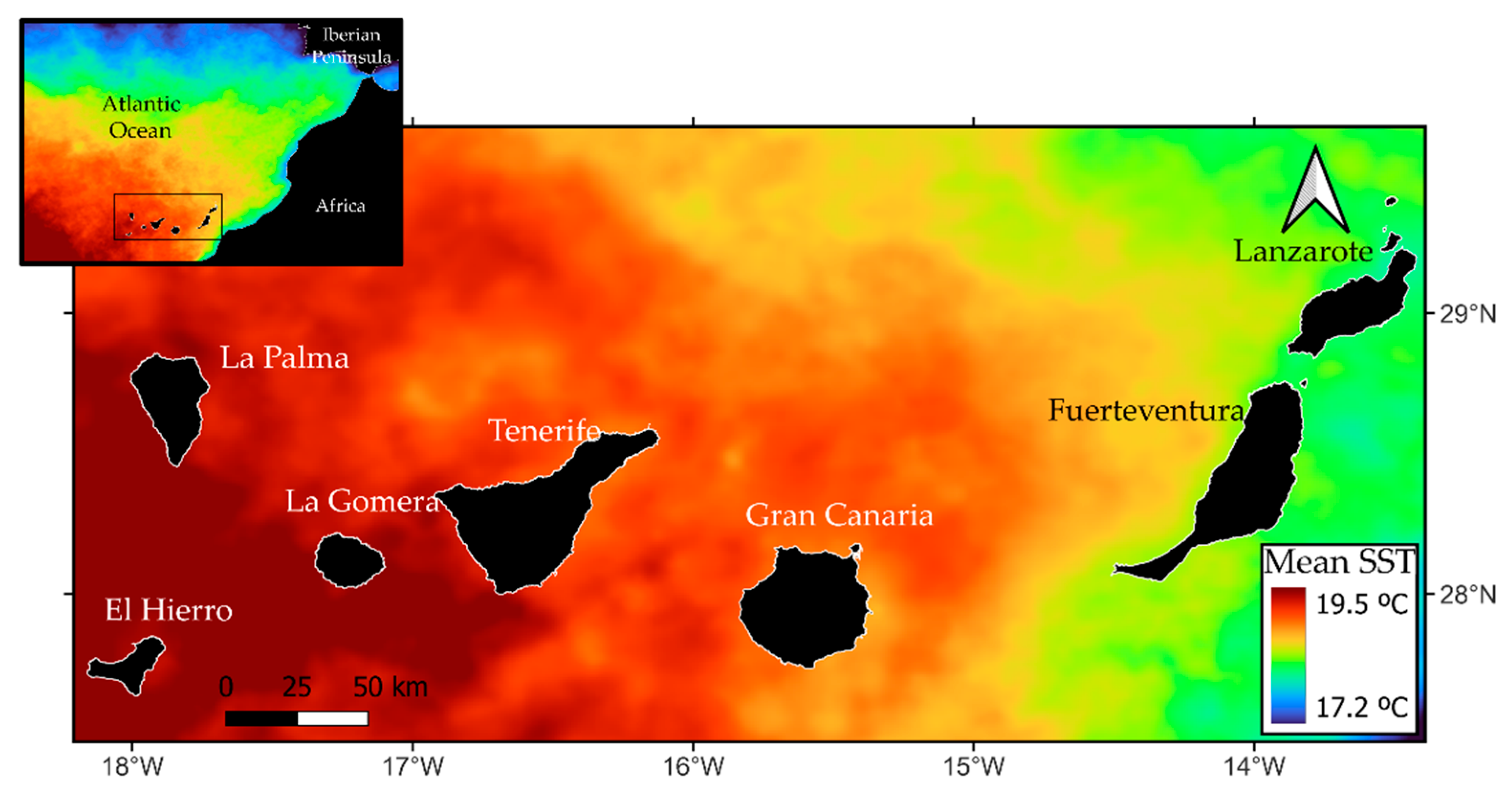
The Canarian Archipelago comprises eight main islands located in the North-east Atlantic (Figure 1). It is a volcanic oceanic archipelago formed progressively from a long-lived magma source over 60 million years.
The islands possess steep bathymetry, with depth profiles abruptly ranging from over 2000 m to narrow shelves, presenting deep channels between islands. In the western regions, we can find the oldest islands, with higher availability of soft substrate, in contrast with the predominant rocky bottoms of the eastern region. The trade winds make the northern and north-eastern slopes the most exposed to waves.
The Canary Islands have a sub-tropical climate with warm temperatures and small seasonal variations. The main large-scale oceanic flow in the Canary Islands is the Canary Current, a relatively cold surface current following the SSW direction [43].
In contrast to the African coast, considered a rich region in fishery production, the Canary Islands are generally characterized by oligotrophic waters, with relatively low primary production rates and limited fishing resources [44]. Nevertheless, close to the transition zone of the Canarian current, eutrophic areas can be found [45] and fishing activities still play an important role from a cultural and socio-economic point of view, as numerous towns and families are dependent on this sector.

2.2. Distribution Model

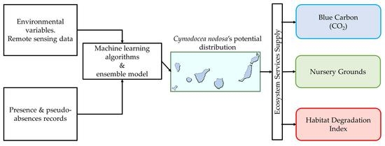
The distribution model of C. nodosa was developed using different machine learning (ML) algorithms with known presence records of the species, along with generated pseudoabsence data. A set of environmental variables retrieved from different freely available RS products were used in the modelling process. The potential Habitat Suitability was constructed from an ensembled model for the whole Canarian archipelago. Finally, the model obtained was used to assess the C. nodosa’s potential ES supply (Figure 2).

2.2.1. Presence and Pseudo-Absence Data

C. nodosa presence records were extracted from historic benthic maps [11,12,13,14,15]. Records were identified as stable meadows and, hence, representative of optimal environmental conditions. A total of 148 presence records were gathered.
Two different groups of pseudo-absence datasets were generated. On the one hand, a series of random localities was pre-selected across the study area as background records, later to be referred to as Aleatory Pseudo-Absences (APA). On the other hand, previously identified areas with a low probability of species occurrence were subsampled [46,47] to define a set later to be referred to as Environmental Pseudo-Absences (EPA).
In the last step, both APA and EPA were randomly subsampled, aiming for different prevalence ratios. Prevalence ratios of 1, 0.5, 0.25, and 0.1 were considered, leading us to create 8 different sets: APA1 and EPA1, with 148 randomly selected respectively, APA0.5 and EPA0.5, with 296 records, APA0.25 and EPA0.25, with 592 records and finally APA0.1 and EPA0.1 with 1480, where subindexes refer to the chosen prevalence for the aleatory subsampling.

2.2.2. Environmental Variables

RS products and images are gaining relevance in the literature due to their proven capacity to improve the capabilities of the seagrass model’s performance and applications [48,49,50]. In addition, topographic information [51] and dynamic oceanographic variables [52,53,54,55] have been commonly used to model seagrass distribution. In this study, a total of 14 potential environmental predictors (Table 1) were taken from available RS products and spatial datasets, considering their known influence on seagrass distribution.
Depth (m) was obtained from a Digital Terrain Model (DTM) with a native resolution of 5 m × 5 m, provided by the Spanish Ministry of Environment (Table 1). Slope (°) and Aspect (Radians) were taken from Depth data. Northness and Eastness (North and East components of Aspect circular direction) were calculated by applying the cosine and the sine to Aspect, respectively (being both dimensionless).
Euclidean distance to the soft substrate (m), indispensable for the species to root, was retrieved from a Benthic bionomic map of the Canarian Archipelago [15]. The Fetch length (m) (used as a proxy to measure the degree of seagrass protection against disturbances and dislodgement) was processed from the DTM using R studio as in [63].
Chlorophyll-a Concentration (mg·m−3) was derived from NASA Level-3 MODIS-Aqua monthly chlorophyll-a concentration. This product is processed using an empirical relationship from in situ measurements and a specific sensor band reflectance ratio (blue-green) with a spatial resolution of 4 km × 4 km (doi:10.5067/AQUA/MODIS/L3M/CHL/2018). Mean values for warm months (September–October) and cold months (February–March) were calculated for a period ranging from 2010 to 2019.
Sea Surface Temperature (SST) was processed from the NASA GHRSST Level 4 MUR Global Foundation Sea Surface Temperature Analysis. This product relies on wavelet functions, and it is based on night-time SST observations from several NASA and in situ observations to provide a 1 km × 1 km product with global coverage with a time span starting in 2002 (doi:10.5067/GHGMR-4FJ04). SST values were considered for a period of time ranging from 2010 to 2019, calculating mean values of warm months (September–October) and cold (February–March) months.
Sea surface wave significant height (SWH, expressed in meters), Sea surface wave mean direction (°) and Sea surface peak period (s) were obtained from the Atlantic-Iberian Biscay Irish-Ocean (IBI) Wave Analysis and Forecast product (doi:10.48670/moi-00027). This product provides modeled wave forecast information with ingested wind and significant wave height altimeter data along with currents from the IBI ocean circulation system. It provides with near real-time observation and forecasts with a spatial resolution of 5 km × 5 km, with data availability starting in 2019 [64]. The maximum wave energy flux (power of wave crest per meter, expressed in kW·m−1) was calculated using values of maximum significant wave height and peak period with R studio 1.1.463 using the waver package [65]. All variables were resampled to 100 m × 100 m resolution.
99th percentile of Significant Wave Height (SWH, expressed in m) was retrieved from the Iberia-Biscay-Ireland Significant Wave Height extreme variability product [66]. This product is constructed with the computation of the annual 99th percentile of SWH from historical records, ranging from 1993 to 2019 with a spatial resolution of 1 km × 1 km.
Environmental predictors’ collinearity was assessed, accounting for non-independence. Unfortunately, even when correlated, variables may not hold just redundant information. To minimize the potential information loss, two steps were followed to ensure that all environmental variables were considered for the later modeling process. First, variables presenting collinearity were identified using a pairwise correlation analysis applying a threshold of 0.8 [67]. All different combinations of correlated and uncorrelated variables were considered, creating a total number of 12 predictor sets by rejecting the possibility of any correlated variables being present in the same group (Table 2). Finally, the pre-selected sets were tested using a Variance Inflation Factor (VIF) analysis, as this test may highlight collinearities sometimes missed in the pairwise correlation analysis [68,69]. VIF analysis showed variable uncorrelation in all 12 sets.

2.2.3. Model Fitting

A series of models were run following two parallel procedures. On the one hand, we used MaxEnt [70], a widely used ML algorithm for modeling species distribution to construct models. In this step, an automated calibration process was carried out using kuenm R package, developed by [71]. This package allows for optimal MaxEnt parameter optimization, creating and evaluating a series of candidate models while incorporating all possible combinations of presence records, environmental pre-selected variable sets, and user-defined algorithm settings. A total of 743 models were run, evaluating each output’s statistical significance. All possible settings for user-defined algorithm parameters were considered, relying on algorithm’s default background selection criterion. Beta multiplier values were set to range from 0.5 to 1.5 with increasing additive steps of 0.1, and all possible combinations of feature class selection were considered in the fitting procedure.
On the other hand, algorithms such as Random Forest (RF), Generalized Additive Models (GAM), Generalized Lineal Model (GLM), and Artificial Neural Networks (ANN) were considered and run within biomod2 R package [72]. This package allows the implementation of a wide range of algorithms, providing tools for model calibration and evaluation while incorporating a series of assessments for model explanatory capabilities and predictive performance. In this step, all combinations between the 4 selected algorithms, 4 Pseudo-absence (EPA), and 4 Background (APA) generated sets led to the implementation of 32 different models. All models were run using the environmental variable sets presenting statistical significance in the previous step. An iterative process was carried out in an empirical search for each algorithm’s user-defined optimal settings.

2.2.4. Model Evaluation

Two different processes were carried out: model validation, used to infer optimal parameter settings and to compare different models’ robustness, and model testing, accounting for predictive accuracy [73].
A 5-fold cross-validation technique with 25% test samples was used [74]. Model validation criteria was based on: (i) Delta Akaike Information Criterion (dAIC) threshold below 2, being this parameter the difference between a particular model’s AIC and the lowest AIC of all candidate models, pointing to models with optimal trade-offs between data fitting and complexity [75] and (ii) Omission rate threshold below 0.05, depicting the proportion of test records incorrectly predicted by the model [76].
To test model predictive accuracy, we relied on (i) Area Under the Curve (AUC), describing the degree of agreement between the model projection and actual occurrence data [77], (ii) Model specificity and sensitivity (proportion of absences and presences correctly predicted by the model, respectively) [78] and (iii) True Skill Statistics (TSS), used to evaluate the model’s predictive performance and accuracy [79], considering a selection threshold value higher than 0.8.

2.2.5. Model Ensemble and Potential Habitat Suitability Mapping

An ensemble model was constructed by averaging the outputs of models selected in the previous valuation step, accounting for robustness, statistical significance, and predictive capabilities. Ensemble modeling is a process in which multiple models are used to predict a single outcome, either by using many different modeling algorithms (such as in our case) or using different training data sets [80]. This technique presents advantages over single-model forecasts [34], and predictive power has been proved to improve when used [81]. The single outcome model was projected to the Canarian archipelago to retrieve a final potential Habitat Suitability Map (HSM) for C. nodosa.

2.3. Assessing Ecosystem Services (ES) Supply

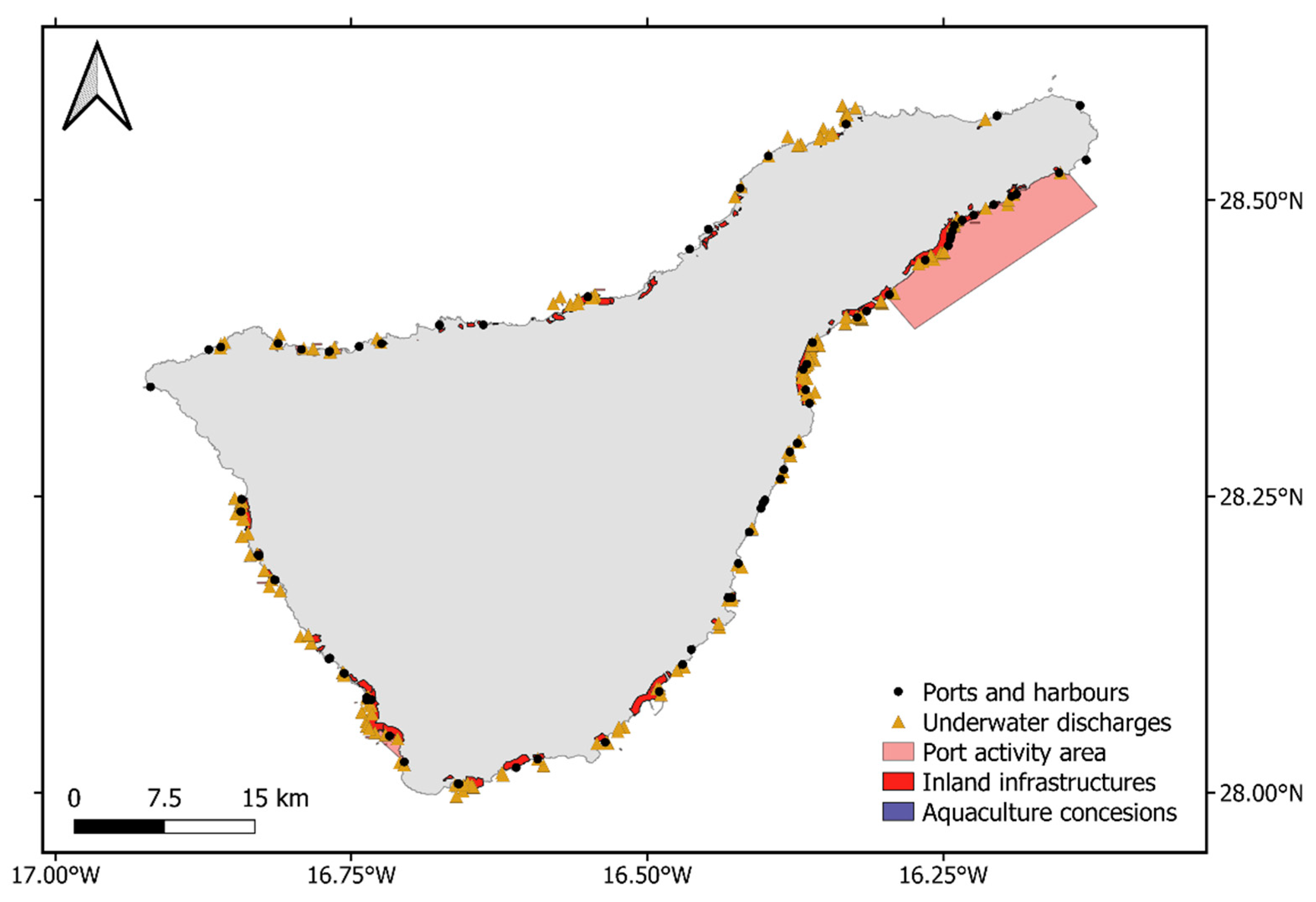
The obtained ensembled model was used for the estimation of the potential ES supply of C. nodosa in the Canarian archipelago. The analysis was carried out with InVEST 3.8.1 software (Integrated Valuation of Ecosystem Services and Trade-offs), a free software developed by the Natural Capital Project [82]. It is a tool for geographic, economic and ecological accounting on ES, aiming to describe and characterize the ecosystem-based goods provision, relying on geographic data describing the biophysical properties of any given habitat/ecosystem [83]. As a first step, Carbon sequestration and the species’ role as nursery grounds for commercially interesting fish species were estimated for the Canarian seagrasses. Then, a degradation index was produced using the InVEST Habitat Quality model. This tool feeds on spatial data depicting potential disturbances to assess the conservation status of any given habitat/ecosystem. Anthropogenic variables affecting seagrass distribution were retrieved from the cartographic service offered by GRAFCAN S.A. (https://www.idecanarias.es/listado_servicios, accessed on 4 July 2022) in collaboration with the Government of Canary Islands (https://datos.canarias.es/portal/datos/, accessed on 4 July 2022). Spatial information regarding aquaculture activities, wastewater discharges, and the presence of ports and coastal infrastructures was used to run the model (Figure 3).
Finally, the degradation index was applied to the ES assessment. This procedure was used to first characterize the ES supply under a hypothetically pristine scenario (depicted by the habitat suitability map). Secondly, it allowed us to compare and assess the potential ES supply loss due to habitat degradation induced by coastal human pressures.

2.3.1. Carbon Stock Estimation

Following the procedure presented in [84], this tool accounts for carbon storage in three “pools”: biomass, sediment, and dead matter (litter). Published C. nodosa’s carbon stocks [40] were used as the main data source, along with the C. nodosa potential distribution map and its related social cost [85], calculated at 48.65 € for 2021 [86], to estimate the amount of CO2 stored and its economic value.

2.3.2. Nursery Grounds Estimation

This ES could be described as the species’ capabilities to sustain a viable population of any particular species. The “fisheries” tool in inVEST uses different data on fish species’ life traits to construct a population dynamics model to assess the economic value of hypothetical fishing activities. Data published by [4], along with databases in “fishbase.org” were used to feed the model and assess the potential economic value of a series of commercially interesting fish species, known to use C. nodosa meadows as nursery grounds. Spatially explicit economic estimations were produced for 6 commercially relevant species in the Canarian Archipelago: Sparisoma cretense, Mullus surmuletus, Pagellus erythrinus, Spondyliosoma cantharus, Diplodus annularis and Dicentrarchus punctatus.

3. Results

3.1. Distribution Model’s Testing and Evaluation

Among 744 different MaxEnt models, 218 matched the omission rate criterion (<0.05), while only one surpassed the dAIC complexity requirements (dAIC < 2). The selected model presented an omission rate of 0.029, dAIC of 0.991, and AIC of 2858.445, showing excellent predictive capabilities with an AUC value of 0.933. Selected features were “Quadratic”, “Product” and “Threshold”, with a Beta multiplier value of 1 (Table 3). The selected MaxEnt model was run with environmental set 5 (Table 2).
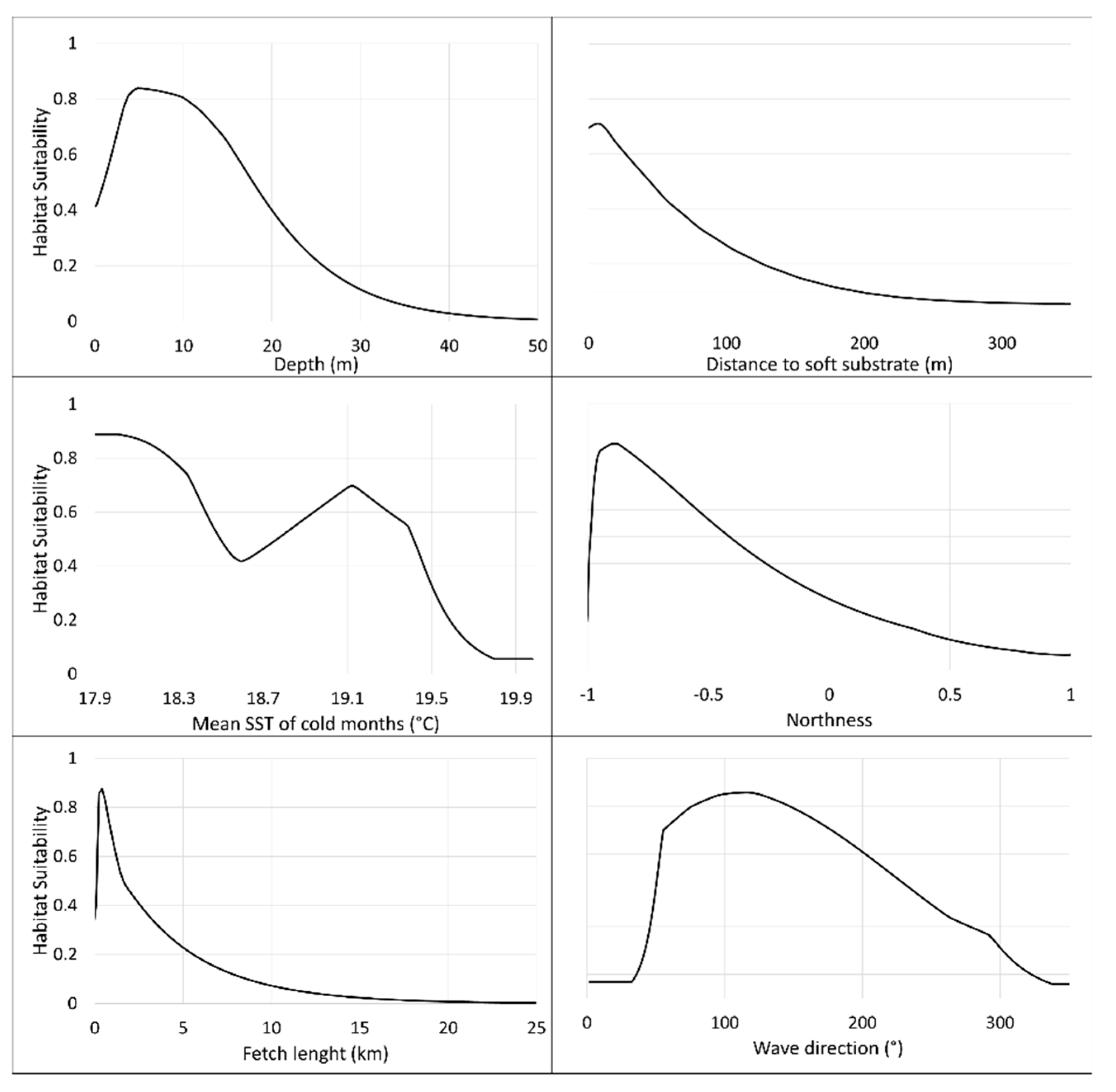
Six predictor variables held 90.6% of the predictive capabilities. Depth, with 59.4% of variable permutation performance, was the variable best explaining C. nodosa’s potential distribution. Distance to the soft substrate, SST, Northness, fetch length and wave mean direction held 31.2% of importance together. The species’ Habitat Suitability response to variability in predictor variables is presented in Figure 4.
A negative correlation was found between species’ habitat suitability and depth, distance to soft substrate, northness, fetch length, and wave direction. The species presents two peaks of habitat suitability around SST values of 18 and 19 °C approximately. Permutation importance and variable’s values related to suitable areas for the species are presented in Table 4.
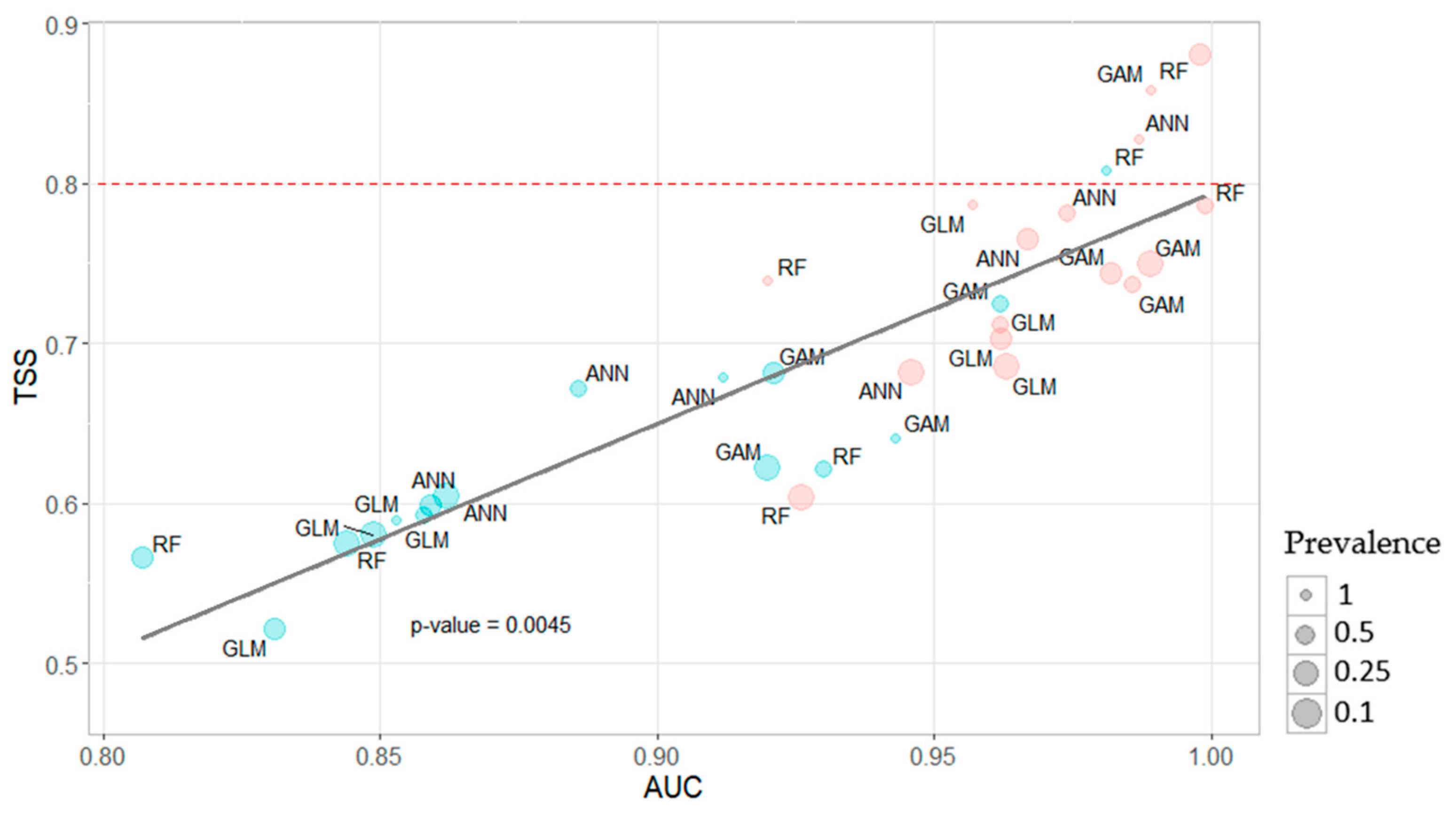
AUC and TSS values for the 32 models relying on user-generated APA and EPA sets are presented in Figure 5.
A correlation between AUC and TSS values was found in both groups of models, with higher values of TSS closely related to higher values of AUC. Overall, AUC values describe good performance, while TSS values are generally lower. Models run with the APA pseudo-absences group presented better performance, with slightly better AUC results. Three different models surpassed the proposed TSS threshold selection criteria, in contrast with the one model in the EPA group. A prevalence value of 1 was present in 3 out of 4 selected models, and 0.25 for the selected EPA model. The selected models were: (i) RF model run with EPA1 (EPA pseudo-absence set with a prevalence of 1), (ii) RF model with APA0.25 (APA pseudo-absence set with a prevalence of 0.25), (iii) GAM model with APA1 (APA pseudo-absence set with a prevalence of 1) and (iv) ANN model with APA1 (APA pseudo-absence set with a prevalence of 1). All evaluation metrics of the selected models are presented in Table 5.
Predictors’ importance was very similar across all selected models to those in the MaxEnt model, pointing out a robust coherence in the results. Six predictor variables held the majority of the predictive capabilities in each model. Mean values across all 4 selected models for permutation importance and value ranges related to suitable areas are presented in Table 6.
On average, 91.2% of variable importance was held by these 6 variables. In contrast to the selected MaxEnt model, fetch length gained more weight (9.43%), surpassing northness (8.93%). Overall, variable importance was more equilibrated, and optimal predictor range values related to species suitability areas were similar to the MaxEnt model.

3.2. Ensemble Model and Potential Habitat Suitability Map

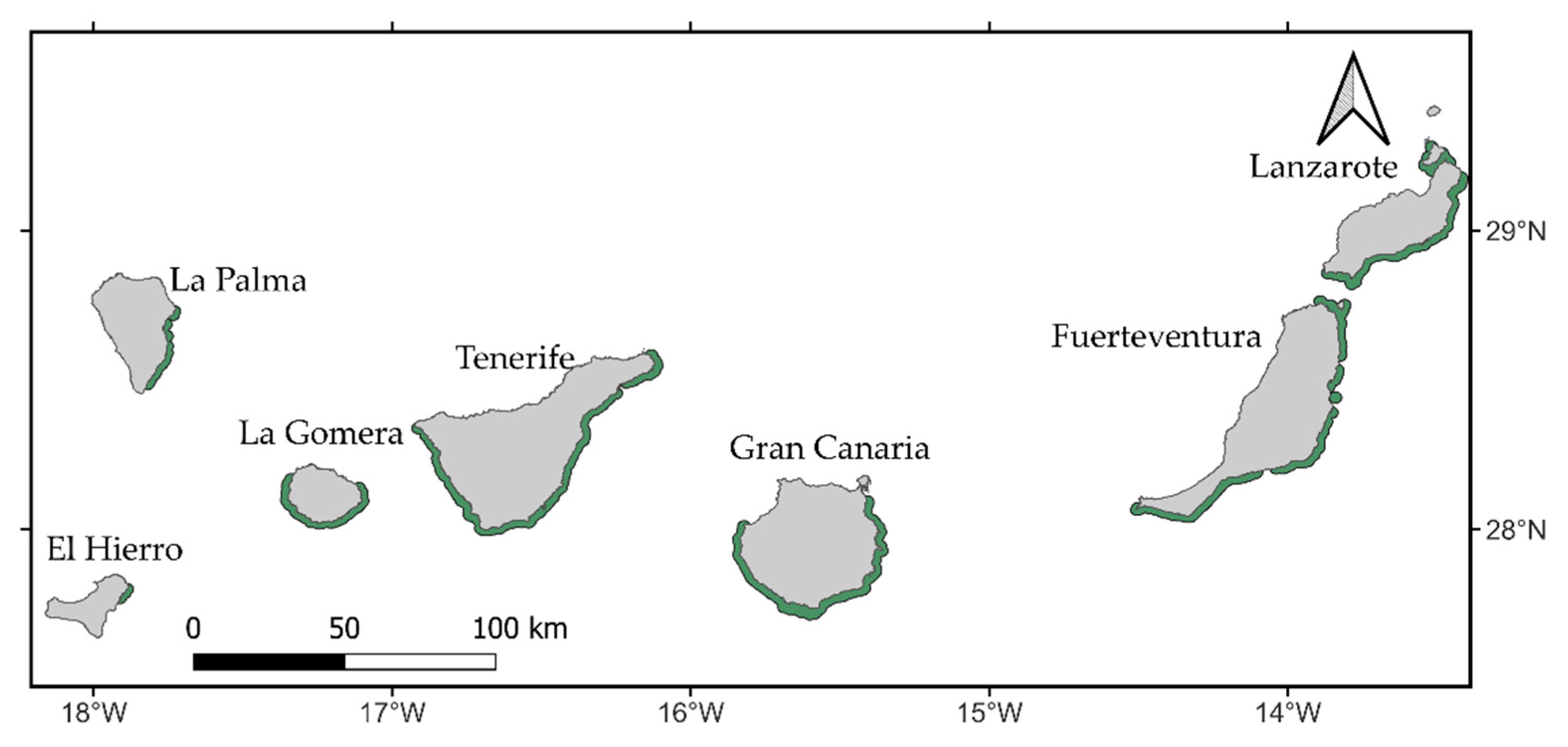
The averaged ensembled model was produced with all previously selected models and projected onto the Canarian archipelago (Figure 6). This projection depicts the spatial distribution of the potentially suitable areas for the species as a response to optimal environmental conditions. Within the study area, 14,047 ha were identified as potentially suitable for the species.
A decreasing pattern in habitat suitability can be described as following an east-west and a north-south trend. Suitable areas are present on the southern coasts, while lower suitability values are found in the western islands, mainly on La Palma and El Hierro.
The species’ suitable areas are closely related to specific value ranges of critical environmental variables (Table 4 and Table 6), constraining the distribution of C. nodosa to these geographic locations. Species’ potentially suitable areas can be found in relatively shallow waters on the south and south-east coasts of the islands, related to low values of northness, with south-east dominant wave direction. Fetch length low values point to a preference for sheltered areas, where the overall wave energy is lower, and occasional extreme events are less likely to impact the species. Sandy bottoms are suitable for C. nodosa, and soft substrate nearby areas are prone to the species’ establishment. The species presents a habitat suitability peak around SST values of 18 °C and a relatively lower suitability peak around 19 °C.

3.3. ES Supply Estimation

The degradation index produced (Figure 7) ranges from 0 in non-disturbed areas, to 1, in most disturbed areas. A total of 4916 ha previously identified as suitable for the species were directly affected by the presence of coastal infrastructures, representing 35% of the total suitable area.
Higher values of degradation appear to be mainly related to the presence of ports and coastal infrastructures. Ports such as Santa Cruz de Tenerife, San Sebastián de La Gomera, Las Palmas de Gran Canaria, Arrecife and Puerto del Rosario seem to have direct impacts on the species’ habitat degradation (Figure 7). On a smaller scale, but visibly noticeable, Santa Cruz de la Palma port also negatively affects C. nodosa’s suitability.

3.3.1. Blue Carbon Sequestration Assessment

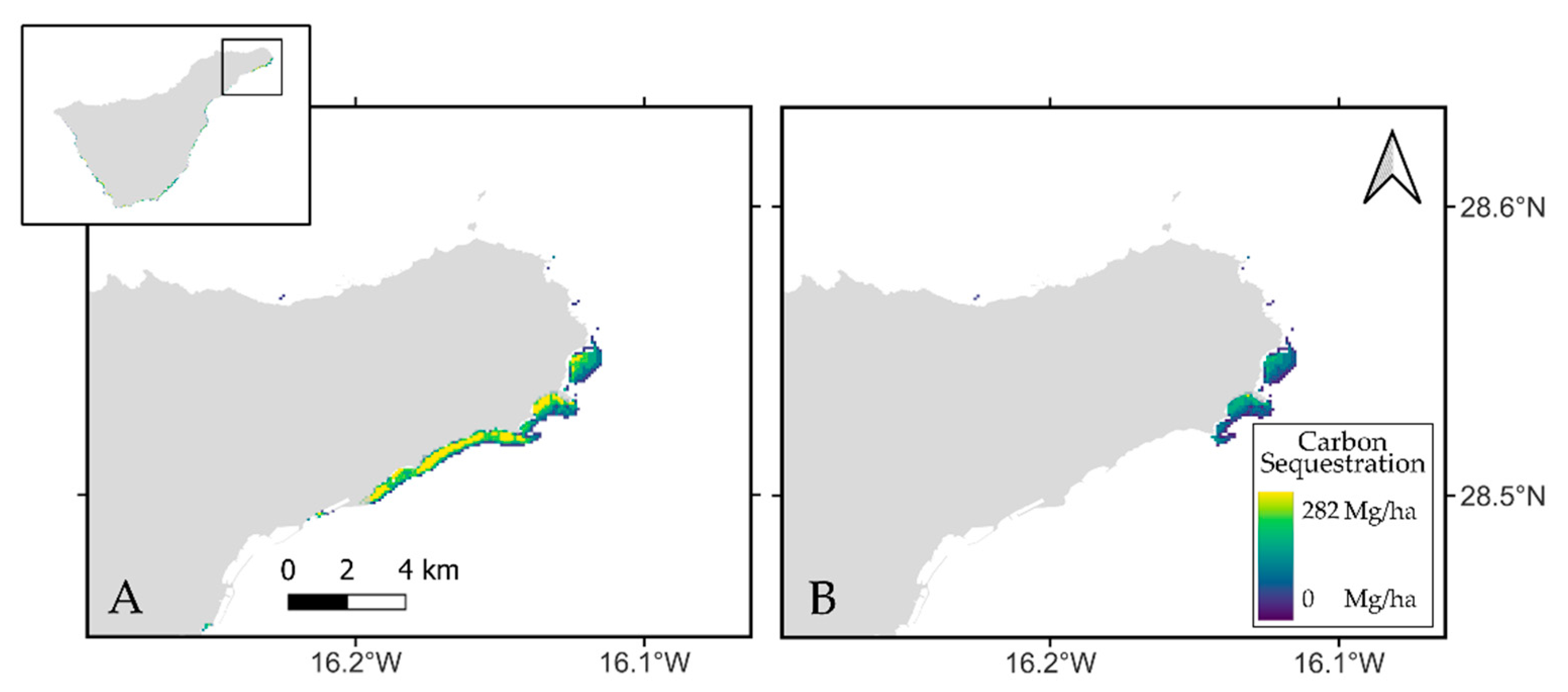
The amount of potential carbon sequestration of C. nodosa was estimated, and a spatially explicit assessment is presented in Figure 8.
The average carbon sequestration was estimated as 282 Mg CO2·ha−1. The total amount of sequestered carbon and its social-economic value is presented in Table 7, both for pristine suitable areas and for the suitability degraded scenario.
The amount of potential sequestered carbon under a pristine scenario was estimated at 3,961,254 Mg CO2, and its social cost was valued at 192,715,007€. These values dropped by approximately 35% after the degradation index was applied, with a potential loss of 1,386,312 Mg of stored carbon resulting in an economic social value decline of 67,444,079€.

3.3.2. Nursery Grounds Assessment

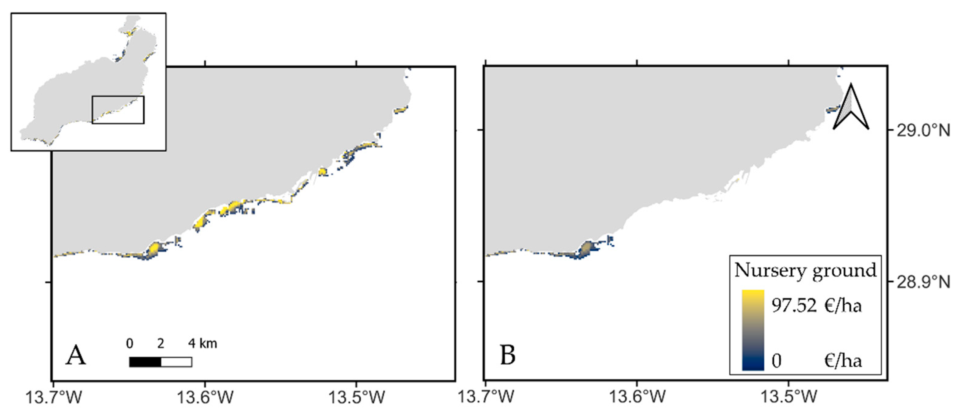
Finally, the spatially explicit economic valuation of C. nodosa’s role as nursery grounds for commercially interesting fish species is presented in Figure 9, both for pristine potential suitable areas and for the degraded scenario. The total economic estimation is presented in Table 8.
The total economic value of C. nodosa as nursery grounds under a pristine scenario was estimated at 1,369,863 €. These values dropped to roughly 35% after the degradation index was applied, with a potential loss of 479,408 €. Sparisoma cretense and Mullus surmuletus were the two best-valued species, due to their relatively high market price, holding 88% of the total economic value. On the other hand, the value of Dicentrarchus punctatus was significantly lower, considering the overall average monetary value of all species (16.25€).

4. Discussion

A distribution model of C. nodosa meadows was produced, being one of the first attempts to apply this methodology in the Canarian Archipelago. Based on the modeled potential distribution of this species, we assessed the ES provision while characterizing the potential impacts of human coastal activities.
On the one hand, the proposed methodology focused on the Canarian Archipelago, and better captured the species particularities in this geographic region than previous modeling attempts, on much broader scales [18]. On the other hand, the modeled distribution allowed us to overcome the intrinsic limitations of the previous cartographies of C. nodosa in terms of technical infeasibility and temporal discrepancies due to the species’ high seasonal variability [17,87].
Only presence records were available for the study, with no true absence records, and we relied on the generation of pseudo-absence data as an alternative. This kind of data may improve model performance [23], while on the other hand allowing the use of standard analysis methods for presence/absence data [19,88]. The generation of pseudo-absence data is a critical process, as it dramatically affects the model’s performance [26]. An unbalanced design with more pseudo-absences than presence records has been found to affect the performance of some models positively, and others negatively [24]. Some studies suggest an optimal prevalence of 0.5 [89], while others lower that ratio down to 0.1 [90]. We considered different types of pseudo-absences and prevalence ratios to cope with this lack of a clear consensus, and the final model selection criteria were based entirely on model performance. For the present modeling procedure, an equilibrated ratio between presences and pseudo-absences was found to yield better results. In one out of three cases, 0.25 was the preferred prevalence, while the rest of the models were run with a prevalence of 1, feeding the narrative of a lack of consensus in this matter. In contrast to some studies highlighting worse performances for models run with aleatory pseudo-absences [91], the majority of the selected models identified as statistically significant were constructed with randomly selected pseudo-absences. Nevertheless, these results are completely in concordance with findings in [24], where better results were obtained when randomly selected pseudo-absences were used with regression modeling techniques. On the other hand, authors found better results when applying environmental-based criteria for pseudo-absence selection with classification techniques, such is the case for the selected RF model in this study, being the only model run with EPA pseudoabsence data.
The environmental variables correlation is another critical step in species distribution modeling, as it negatively affects the model’s performance. VIF analysis was used in addition to pairwise correlation, as it proved to highlight correlation sometimes missed by pairwise analyses [92,93]. The approach followed, combined with the construction of different sets of environmental variables, allowed us to minimize the information loss, a method recognized as capable of improving the model’s performance [71] but still not commonly used in species distribution models [94].
In general, evaluation metrics for MaxEnt models were very robust, and the selected model outperformed all the other candidates, showing very consistent values of AUC, AIC, and omission rates. The rest of the models based on pseudo-absence data presented robust AUC, specificity, and sensitivity, pointing to a balanced trade-off between commission and omission errors, while TSS was generally lower.
Traditional model evaluation approaches using metrics such as AUC have been criticized for not being a strong metric on its own [95], so we considered a wide range of evaluation metrics, aiming for scrupulous filtering of candidate models, highlighting the role of dAIC as a strong metric [96,97], as well as omission rate [98]. Two out of four selected models used RF algorithm, in concordance with recent findings [99,100], feeding the narrative that RF models presented especially good performances when applied to seagrass distribution models [53].
The results regarding predictors’ importance are robust and consistent in all selected models. In all cases, the same six environmental variables held more than 90% of models’ predictive capabilities (Depth, distance to the soft substrate, mean SST of cold months, northness, fetch length, and wave direction), although variable importance was generally more equilibrated for models run with pseudo-absence data.
Depth and fetch length shaped the potential distribution area for the species to shallow waters, relatively sheltered, while northness and wave direction delimited the potential suitable areas to the south-eastern coasts of the islands. The western region of the archipelago presents lower suitability for the species, as island geological age, following an east-to-west direction, is directly related to substrate availability. Variations in SST values also follow an east-to-west increasing trend, with differences between western and eastern regions up to 5 °C [101], mainly due to the influence of the upwelling of the African coast [45], which may cause differences in the longitudinal distribution of some species. The first peak of habitat suitability around lower values of SST could be explained by the proximity of the eastern islands to the aforementioned upwelling of the African coast. These islands present the lowest values of SST. The second peak of habitat suitability starts around 19 °C and decreases when values of SST tend to increase, as these higher values are found in the western regions of the archipelago. These results show that the SST does not seem to be a key variable for the survival of the species in the Canary Islands, and contrast with findings in [18], in which SST winter optimal values for the establishment of the species seem to be lower (around 14 °C). Although it has been suggested that the global loss of meadows has been partly caused by climate change [102], this phenomenon has mainly concerned Mediterranean meadows formed by Posidonia and Zostera species. Caution is advised when comparing the results between models, as different study scales are known to lead to different variable importance [73,103]. There is still no evidence that it affects C. nodosa in the same way, and it has even been suggested that C. nodosa may even benefit from global warming due to its affinity for warm waters [104]. Nevertheless, there are other mechanisms linked to climate change, rather than temperature, that may have a significant impact on C. nodosa meadows, such as the increasing frequency and intensity of extreme weather events.
The consistency and robustness of the different models, regarding variables’ importance and predictive capabilities, allowed for the construction of an ensemble model. It is known to have the potential of improving model robustness over attempts using single algorithms [33,34], while enhancing our model’s prediction confidence [35]. Even though the ensemble model was constructed with multiple base models, it performed as a single species distribution model.
A total of 14,047 ha were identified as potentially suitable for the species, in contrast with the 6709 ha in the Canary islands occupied by C. nodosa meadows as stated in the Marine Phanerogams Atlas from Spain [105]. This is an expected discrepancy as these 14,047 ha refer to potential areas for the species to establish, considering no human presence whatsoever. Coastal infrastructures such as ports are usually placed in naturally sheltered areas, also preferred for the species to establish, and habitat suitability in areas surrounding these infrastructures was especially jeopardized. After the degradation index was applied, the total suitable area decreased to 9131 ha, much closer to the values found in the Marine Phanerogams Atlas from Spain. It is likely that the coastal activities dataset lacked information about human impacts influencing the species distribution, mainly due to data availability, but it still allowed us to better comprehend the scope of the potential habitat loss due to these kinds of coastal impacts.
This study represents the first attempt to estimate the monetary value of both Blue carbon and Nursery grounds at an archipelago scale in the Canary Islands. For the species studied, we estimated the monetary value for C. nodosa’s role as nursery grounds at 97.52 €*ha−1, a slightly higher value compared to previous studies (89.13 €*ha−1) [4]. This value was then estimated at 1,369,863 € for the whole archipelago considering a pristine scenario, and 890,455 € after the degradation index was applied. The economic estimation of C. nodosa’s role as nursery grounds is extremely difficult to compare with the known real economic valuation of coastal fisheries (https://www.gobiernodecanarias.org/agp/sgt/galerias/doc/estadisticas/pesca/2007_2021-especie_meses-valor.ods, accessed on 4 July 2022). These published values relate to the economic market profit of the extracted fish, which represent a small fraction of the whole fish population. The economic estimation presented in this study relates to the total potential economic value of the whole fish stocks that use C. nodosa as nursery ground, and both assessments refer to different Ecosystem Services. Nevertheless, the value of this work lies especially in highlighting the economic loss of ES for Cymodocea meadows in the Canary Islands as a whole, which is a result to be taken into account in future decision-making for the management of these communities.
The Blue Carbon estimations presented in this study are very consistent with previous studies using similar methodologies [40], where they assessed the carbon stock related to this species in 3,173,469 Mg. Our estimations resulted in 3,961,254 Mg CO2 and this stock was then valued at 192,715,007€. When considering a degraded scenario, these values dropped down to 2,574,942 Mg CO2, resulting in an economic assessment of 125,270,928€. Overall, studies assessing the monetary social value of carbon stocks in different regions and other seagrass species, present certain discrepancies. ES economic values carried out for the Spanish territory [40] are lower than for the European region [106], which is probably related to the use of different carbon prices, induced by carbon price instability over time and the regional particularities of the species studied.

5. Conclusions

The analysis of the input parameters of the modeling, as well as the application of different algorithms, allowed us to obtain a reliable and representative distribution model of the potential habitat of Cymodocea nodosa. This model provides us with valuable information not only about its distribution in pristine conditions but also about the relationship of the species with the environmental variables analyzed.
At the same time, the distribution model allowed us to quantify the impact of human activities on this species and its ES provision. Our results, although based only on two ES, demonstrate its great socio-economic importance, setting precedents and highlighting the need for further studies of this kind.
The degraded habitat produced in this study, although approaching a realistic scenario for the distribution of the species in the archipelago, needs to be further explored. Many variables describing other types of human activities jeopardizing the distribution of C. nodosa have not been taken into account and should be taken into consideration for future studies. However, the proposed methodology helps us to understand in greater depth the capabilities that this type of analysis offers.
This methodology allowed us to observe the decrease in habitat suitability in a spatially explicit way, being a very useful tool for policy decision support, which has been overlooked, especially in European ORs. One of the reasons for the lack of studies that consider the spatially explicit dimension of ES assessments, as well as the geographical distribution of the different human impacts on the coast, is the availability of data. In this sense, the use of RS products and imagery is presented as a valuable tool to overcome this limitation.
Author Contributions

Conceptualization and methodology, E.C., L.M.-G. and M.A.; formal analysis, writing—original draft preparation and writing—review and editing, E.C., L.M.-G., M.A. and P.H.-L.; software, E.C.; funding acquisition, M.A. and P.H.-L. All authors have read and agreed to the published version of the manuscript.

Funding

This research was developed while the corresponding author (Enrique Casas) had a contract within the predoctoral program for the training of research personnel in the Canary Islands, financed by the European social fund and the government of the Canary Islands.

Data Availability Statement

The data presented in this study are available on request from the corresponding author. The data are not publicly available due to privacy issues.

Acknowledgments

The authors thank Leopoldo Moro (Gobierno de Canarias) and Jose María Espinosa (Observatorio Ambiental de Granadilla) for their collaboration in the databases used in the framework of this project.

Conflicts of Interest

The authors declare no conflict of interest.

References

  1. Green, E.P.; Short, F.T. World Atlas of Seagrasses; University of California Press: Berkeley, CA, USA, 2003. [Google Scholar]
  2. Nordlund, L.M.; Jackson, E.L.; Nakaoka, M.; Samper-Villarreal, J.; Beca-Carretero, P.; Creed, J.C. Seagrass Ecosystem Services—What’s Next? Mar. Pollut. Bull. 2018, 134, 145–151. [Google Scholar] [CrossRef] [PubMed]
  3. Nordlund, L.M.; Unsworth, R.K.F.; Gullström, M.; Cullen-Unsworth, L.C. Global Significance of Seagrass Fishery Activity. Fish Fish. 2018, 19, 399–412. [Google Scholar] [CrossRef]
  4. Tuya, F.; Haroun, R.; Espino, F. Economic Assessment of Ecosystem Services: Monetary Value of Seagrass Meadows for Coastal Fisheries. Ocean Coast. Manag. 2014, 96, 181–187. [Google Scholar] [CrossRef]
  5. Waycott, M.; Duarte, C.M.; Carruthers, T.J.B.; Orth, R.J.; Dennison, W.C.; Olyarnik, S.; Calladine, A.; Fourqurean, J.W.; Heck, K.L.; Hughes, A.R.; et al. Accelerating Loss of Seagrasses across the Globe Threatens Coastal Ecosystems. Proc. Natl. Acad. Sci. USA 2009, 106, 12377–12381. [Google Scholar] [CrossRef]
  6. Short, F.T.; Polidoro, B.; Livingstone, S.R.; Carpenter, K.E.; Bandeira, S.; Bujang, J.S.; Calumpong, H.P.; Carruthers, T.J.B.; Coles, R.G.; Dennison, W.C.; et al. Extinction Risk Assessment of the World’s Seagrass Species. Biol. Conserv. 2011, 144, 1961–1971. [Google Scholar] [CrossRef]
  7. Jordà, G.; Marbà, N.; Duarte, C.M. Mediterranean Seagrass Vulnerable to Regional Climate Warming. Nat. Clim. Chang. 2012, 2, 821–824. [Google Scholar] [CrossRef]
  8. González-Correa, J.M.; Bayle Sempere, J.T.; Sánchez-Jerez, P.; Valle, C. Posidonia Oceanica Meadows Are Not Declining Globally. Analysis of Population Dynamics in Marine Protected Areas of the Mediterranean Sea. Mar. Ecol. Prog. Ser. 2007, 336, 111–119. [Google Scholar] [CrossRef]
  9. Afonso, J.; Gil, M.C. Cymodocea nodosa (Ucria) Ascherson (Zannichelliaceae) y Las Praderas Submarinas o “Sebadales” En El Archipiélago Canario. Vieraea 1980, 8, 365–376. [Google Scholar]
  10. Oliva, S.; Mascaró, O.; Llagostera, I.; Pérez, M.; Romero, J. Selection of Metrics Based on the Seagrass Cymodocea nodosa and Development of a Biotic Index (CYMOX) for Assessing Ecological Status of Coastal and Transitional Waters. Estuar. Coast. Shelf Sci. 2012, 114, 7–17. [Google Scholar] [CrossRef]
  11. Tuya, F.; Ribeiro-Leite, L.; Arto-Cuesta, N.; Coca, J.; Haroun, R.; Espino, F. Decadal Changes in the Structure of Cymodocea nodosa Seagrass Meadows: Natural vs. Human Influences. Estuar. Coast. Shelf Sci. 2014, 137, 41–49. [Google Scholar] [CrossRef]
  12. Reyes, J.; Sansón, M.; Afonso-Carrillo, J. Distribution and Reproductive Phenology of the Seagrass Cymodocea nodosa (Ucria) Ascherson in the Canary Islands. Aquat. Bot. 1995, 50, 171–180. [Google Scholar] [CrossRef]
  13. Barbera, C.; Tuya, F.; Boyra, A.; Sanchez-Jerez, P.; Blanch, I.; Haroun, R.J. Spatial Variation in the Structural Parameters of Cymodocea nodosa Seagrass Meadows in the Canary Islands: A Multiscaled Approach. Bot. Mar. 2005, 48, 122–126. [Google Scholar] [CrossRef]
  14. Barquín-Diez, J.; González-Lorenzo, G.; Martín-Garc¡a, L.; Gil-Rodr¡guez, M.C.; Brito-Hernández, A. Distribución Espacial de Las Comunidades Bent¢nicas Submareales de Los Fondos Someros de Canarias. I: Las Comunidades de Sustrato Blando de Las Costas de Tenerife. Vieraea 2005, 33, 435–448. [Google Scholar]
  15. Martín-García, L.; Sangil, C.; Brito, A.; Barquín-Diez, J. Identification of Conservation Gaps and Redesign of Island Marine Protected Areas. Biodivers. Conserv. 2015, 24, 511–529. [Google Scholar] [CrossRef]
  16. Casas, E.; Martín-García, L.; Otero-Ferrer, F.; Tuya, F.; Haroun, R.; Arbelo, M. Economic Mapping and Assessment of Cymodocea nodosa Meadows as Nursery Grounds for Commercially Important Fish Species. A Case Study in the Canary Islands. One Ecosyst. 2021, 6, 70919. [Google Scholar] [CrossRef]
  17. Guidetti, P.; Lorenti, M.; Buia, M.C.; Mazzella, L. Temporal Dynamics and Biomass Partitioning in Three Adriatic Seagrass Species: Posidonia Oceanica, Cymodocea nodosa, Zostera Marina. Mar. Ecol. 2002, 23, 51–67. [Google Scholar] [CrossRef]
  18. Chefaoui, R.M.; Assis, J.; Duarte, C.M.; Serrão, E.A. Large-Scale Prediction of Seagrass Distribution Integrating Landscape Metrics and Environmental Factors: The Case of Cymodocea nodosa (Mediterranean–Atlantic). Estuaries Coasts 2016, 39, 123–137. [Google Scholar] [CrossRef]
  19. Elith, J.; Leathwick, J.R. Species Distribution Models: Ecological Explanation and Prediction across Space and Time. Annu. Rev. Ecol. Evol. Syst. 2009, 40, 677–697. [Google Scholar] [CrossRef]
  20. Loiselle, B.A.; Howell, C.A.; Graham, C.H.; Goerck, J.M.; Brooks, T.; Smith, K.G.; Williams, P.H. Avoiding Pitfalls of Using Species Distribution Models in Conservation Planning. Conserv. Biol. 2003, 17, 1591–1600. [Google Scholar] [CrossRef]
  21. Warton, D.I.; Shepherd, L.C. Poisson Point Process Models Solve the “Pseudo-Absence Problem” for Presence-Only Data in Ecology. Ann. Appl. Stat. 2010, 4, 1383–1402. [Google Scholar] [CrossRef]
  22. Elith, J.; Leathwick, J. Predicting Species Distributions from Museum and Herbarium Records Using Multiresponse Models Fitted with Multivariate Adaptive Regression Splines. Divers. Distrib. 2007, 13, 265–275. [Google Scholar] [CrossRef]
  23. Stockwell, D.; Peters, D. The GARP Modelling System: Problems and Solutions to Automated Spatial Prediction. Int. J. Geogr. Inf. Sci. 1999, 13, 143–158. [Google Scholar] [CrossRef]
  24. Barbet-Massin, M.; Jiguet, F.; Albert, C.H.; Thuiller, W. Selecting Pseudo-absences for Species Distribution Models: How, Where and How Many? Methods Ecol. Evol. 2012, 3, 327–338. [Google Scholar] [CrossRef]
  25. Senay, S.D.; Worner, S.P.; Ikeda, T. Novel Three-Step Pseudo-Absence Selection Technique for Improved Species Distribution Modelling. PLoS ONE 2013, 8, 71218. [Google Scholar] [CrossRef]
  26. Zaniewski, A.E.; Lehmann, A.; Overton, J.M.C. Predicting Species Spatial Distributions Using Presence-Only Data: A Case Study of Native New Zealand Ferns. Ecol. Modell. 2002, 157, 261–280. [Google Scholar] [CrossRef]
  27. Tracy, J.L.; Trabucco, A.; Lawing, A.M.; Giermakowski, J.T.; Tchakerian, M.; Drus, G.M.; Coulson, R.N. Random Subset Feature Selection for Ecological Niche Models of Wildfire Activity in Western North America. Ecol. Modell. 2018, 383, 52–68. [Google Scholar] [CrossRef]
  28. Diniz Filho, J.A.F.; Ferro, V.G.; Santos, T.; Nabout, J.C.; Dobrovolski, R.; De Marco, P., Jr. The Three Phases of the Ensemble Forecasting of Niche Models: Geographic Range and Shifts in Climatically Suitable Areas of Utetheisa Ornatrix (Lepidoptera, Arctiidae). Rev. Bras. Entomol. 2010, 54, 339–349. [Google Scholar] [CrossRef]
  29. Scales, K.L.; Miller, P.I.; Ingram, S.N.; Hazen, E.L.; Bograd, S.J.; Phillips, R.A. Identifying Predictable Foraging Habitats for a Wide-Ranging Marine Predator Using Ensemble Ecological Niche Models. Divers. Distrib. 2016, 22, 212–224. [Google Scholar] [CrossRef]
  30. Diniz Filho, J.A.F.; Nabout, J.C.; Bini, L.M.; Loyola, R.D.; Rangel, T.F.; Nogues-Bravo, D.; Araújo, M.B. Ensemble Forecasting Shifts in Climatically Suitable Areas for Tropidacris Cristata (Orthoptera: Acridoidea: Romaleidae). Insect Conserv. Divers. 2010, 3, 213–221. [Google Scholar]
  31. Diniz Filho, J.A.F.; Rodrigues, H.; Telles, M.P.D.C.; Oliveira, G.G.; Terrible, L.C.; Soares, T.N.; Nabout, J.C. Correlation between Genetic Diversity and Environmental Suitability: Taking Uncertainty from Ecological Niche Models into Account. Mol. Ecol. Resour. 2015, 15, 1059–1066. [Google Scholar] [CrossRef]
  32. Henrys, P.A.; Smart, S.M.; Rowe, E.C.; Jarvis, S.G.; Fang, Z.; Evans, C.D.; Emmett, B.A.; Butler, A. Niche Models for British Plants and Lichens Obtained Using an Ensemble Approach. New J. Bot. 2015, 5, 89–100. [Google Scholar] [CrossRef]
  33. Kaky, E.; Nolan, V.; Alatawi, A.; Gilbert, F. A Comparison between Ensemble and MaxEnt Species Distribution Modelling Approaches for Conservation: A Case Study with Egyptian Medicinal Plants. Ecol. Inform. 2020, 60, 101150. [Google Scholar] [CrossRef]
  34. Araújo, M.B.; New, M. Ensemble Forecasting of Species Distributions. Trends Ecol. Evol. 2007, 22, 42–47. [Google Scholar] [CrossRef]
  35. Marmion, M.; Parviainen, M.; Luoto, M.; Heikkinen, R.K.; Thuiller, W. Evaluation of Consensus Methods in Predictive Species Distribution Modelling. Divers. Distrib. 2009, 15, 59–69. [Google Scholar] [CrossRef]
  36. Böhnke-Henrichs, A.; Baulcomb, C.; Koss, R.; Hussain, S.S.; de Groot, R.S. Typology and Indicators of Ecosystem Services for Marine Spatial Planning and Management. J. Environ. Manag. 2013, 130, 135–145. [Google Scholar] [CrossRef]
  37. Hattam, C.; Atkins, J.P.; Beaumont, N.; Börger, T.; Böhnke-Henrichs, A.; Burdon, D.; De Groot, R.; Hoefnagel, E.; Nunes, P.A.L.D.; Piwowarczyk, J.; et al. Marine Ecosystem Services: Linking Indicators to Their Classification. Ecol. Indic. 2015, 49, 61–75. [Google Scholar] [CrossRef]
  38. Wilberg, M.J.; Miller, T.J. Comment on “Impacts of Biodiversity Loss on Ocean Ecosystem Services”. Science 2007, 316, 787–791. [Google Scholar] [CrossRef]
  39. Ruiz-Frau, A.; Gelcich, S.; Hendriks, I.E.; Duarte, C.M.; Marbà, N. Current State of Seagrass Ecosystem Services: Research and Policy Integration. Ocean Coast. Manag. 2017, 149, 107–115. [Google Scholar] [CrossRef]
  40. González-García, A.; Arias, M.; García-Tiscar, S.; Alcorlo, P.; Santos-Martín, F. National Blue Carbon Assessment in Spain Using InVEST: Current State and Future Perspectives. Ecosyst. Serv. 2022, 53, 101397. [Google Scholar] [CrossRef]
  41. Maren Sieber, I.; Av Borges, P.; Burkhard, B. Hotspots of Biodiversity and Ecosystem Services: The Outermost Regions and Overseas Countries and Territories of the European Union. One Ecosyst. 2018, 3, 24719. [Google Scholar] [CrossRef]
  42. Borges, P.A.V.; Azevedo, E.B.; Borba, A.; Dinis, F.O.; Gabriel, R.; Silva, E. Ilhas Oceânicas; Escolar: Lisboa, Portugal, 2009; ISBN 978-972-592-274-3. [Google Scholar]
  43. Fiekas, V.; Elken, J.; Muller, T.J.; Aitsam, A.; Zenk, W. A View of the Canary Basin Thermocline Circulation in Winter. J. Geophys. Res. 1992, 97, 12495–12510. [Google Scholar] [CrossRef]
  44. Braun, J.G. Estudios de produccion en aguas de las Islas Canarias I-Hidrografia, nutrientes y produccion primaria. Bol. Inst. Esp. Oceanogr. 1980, 5, 147–154. [Google Scholar]
  45. Barton, E.D.; Aristegui, J.; Tett, P.; Canton, M.; García-Braun, J.; Hernández-León, S.; Nykjaer, L.; Almeida, C.; Almunia, J.; Ballesteros, S.; et al. The Transition Zone of the Canary Current Upwelling Region. Prog. Oceanogr. 1998, 41, 455–504. [Google Scholar] [CrossRef]
  46. Engler, R.; Guisan, A.; Rechsteiner, L. An Improved Approach for Predicting the Distribution of Rare and Endangered Species from Occurrence and Pseudo-Absence Data. J. Appl. Ecol. 2004, 41, 263–274. [Google Scholar] [CrossRef]
  47. Lobo, J.M.; Verdú, J.R.; Numa, C. Environmental and Geographical Factors Affecting the Iberian Distribution of Flightless Jekelius Species (Coleoptera: Geotrupidae). Divers. Distrib. 2006, 12, 179–188. [Google Scholar] [CrossRef]
  48. He, K.S.; Bradley, B.A.; Cord, A.F.; Rocchini, D.; Tuanmu, M.N.; Schmidtlein, S.; Turner, W.; Wegmann, M.; Pettorelli, N. Will Remote Sensing Shape the next Generation of Species Distribution Models? Remote Sens. Ecol. Conserv. 2015, 1, 4–18. [Google Scholar] [CrossRef]
  49. Leitão, P.J.; Santos, M.J. Improving Models of Species Ecological Niches: A Remote Sensing Overview. Front. Ecol. Evol. 2019, 7, 9. [Google Scholar] [CrossRef]
  50. Kachelriess, D.; Wegmann, M.; Gollock, M.; Pettorelli, N. The Application of Remote Sensing for Marine Protected Area Management. Ecol. Indic. 2014, 36, 169–177. [Google Scholar] [CrossRef]
  51. Hastings, R.; Cummins, V.; Holloway, P. Assessing the Impact of Physical and Anthropogenic Environmental Factors in Determining the Habitat Suitability of Seagrass Ecosystems. Sustainability 2020, 12, 8302. [Google Scholar] [CrossRef]
  52. Bittner, R.E.; Roesler, E.L.; Barnes, M.A. Using Species Distribution Models to Guide Seagrass Management. Estuar. Coast. Shelf Sci. 2020, 240, 106790. [Google Scholar] [CrossRef]
  53. Hu, W.; Zhang, D.; Chen, B.; Liu, X.; Ye, X.; Jiang, Q.; Zheng, X.; Du, J.; Chen, S. Mapping the Seagrass Conservation and Restoration Priorities: Coupling Habitat Suitability and Anthropogenic Pressures. Ecol. Indic. 2021, 129, 107960. [Google Scholar] [CrossRef]
  54. Downie, A.L.; Von Numers, M.; Boström, C. Influence of Model Selection on the Predicted Distribution of the Seagrass Zostera Marina. Estuar. Coast. Shelf Sci. 2013, 121, 8–19. [Google Scholar] [CrossRef]
  55. Beca-Carretero, P.; Varela, S.; Stengel, D.B. A Novel Method Combining Species Distribution Models, Remote Sensing, and Field Surveys for Detecting and Mapping Subtidal Seagrass Meadows. Aquat. Conserv. Mar. Freshw. Ecosyst. 2020, 30, 1098–1110. [Google Scholar] [CrossRef]
  56. Ministerio Medio Ambiente (Ed.) Estudio Ecocartográfico del Litoral de Las Islas de Lanzarote, Graciosa y Alegranza (Las Palmas). In Dirección General de Costas; Plan de Ecocartografías del litoral español; Ministerio Medio Ambiente: Madrid, España, 2001. [Google Scholar]
  57. Ministerio Medio Ambiente (Ed.) Estudio Ecocartogrfico de la zona sur del litoral de la Isla de Gran Canaria (Las Palmas). In Secretaría de Estado de Aguas y Costas; Dirección General de Costas; Plan de Ecocartografías del litoral español; Ministerio Medio Ambiente: Madrid, España, 2001. [Google Scholar]
  58. Ministerio Medio Ambiente (Ed.) Estudio Ecocartográfico del litoral de la Isla de La Palma (Tenerife). In Dirección General de Costas; Plan de Ecocartografías del litoral español; Ministerio Medio Ambiente: Madrid, España, 2003. [Google Scholar]
  59. Ministerio Medio Ambiente (Ed.) Estudio Ecocartográfico del litoral de las islas de Fuerteventura y Lobos (Las Palmas). In Dirección General de Costas; Plan de Ecocartografías del litoral español; Ministerio Medio Ambiente: Madrid, España, 2004. [Google Scholar]
  60. Ministerio Medio Ambiente (Ed.) Estudio Ecocartográfico del litoral de la isla de La Palma. In Dirección General de Costas; Plan de Ecocartografías del litoral español; Ministerio Medio Ambiente: Madrid, España, 2005. [Google Scholar]
  61. Ministerio Medio Ambiente (Ed.) Estudio Ecocartofráfico del la zona norte del litoral de la isla de Gran Canaria. In Dirección General de Costas; lan de Ecocartografías del litoral español; PMinisterio Medio Ambiente: Madrid, España, 2005. [Google Scholar]
  62. Martín-García, L.; Barquín-Diez, J.; Brito-Izquierdo, I.T. Atlas Bionómico de Las Islas Canarias; Recopilación de Los Estudios Ecocartográficos de Las Costas Canarias; Ministerio De Agricultura y Pesca, Alimentación y Medio Ambiente: Madrid, Spain, 2016; ISBN 280-16-322-7. [Google Scholar]
  63. Yesson, C.; Bush, L.E.; Davies, A.J.; Maggs, C.A.; Brodie, J. Large Brown Seaweeds of the British Isles: Evidence of Changes in Abundance over Four Decades. Estuar. Coast. Shelf Sci. 2015, 155, 167–175. [Google Scholar] [CrossRef] [Green Version]
  64. Sotillo, M.G.; Levier, B.; Lorente, P.; Guihou, K.; Aznar, R.; Amo, A.; Ghantous, M. Quality information document for Atlantic-Iberian Biscay Irish-Ocean Physics Analysis and Forecasting Product (CMEMS-IBI-QUID-005-001), Copernicus Marine Environment Monitoring Service. Tech, rep. 2021. Available online: https://catalogue.marine.copernicus.eu/documents/QUID/CMEMS-IBI-QUID-005-001.pdf (accessed on 4 July 2022).
  65. Marchand, P.; David, G. Waver: Calculate Fetch and Wave Energy. R Package Version 0.2.1. Cran 2018, 1, 1–6. [Google Scholar]
  66. Lorente, P.; Sotillo, M.G.; Aouf, L.; Amo-Baladrón, A.; Barrera, E.; Dalphinet, A.; Toledano, C.; Rainaud, R.; De Alfonso, M.; Piedracoba, S.; et al. ExtremeWave Height Events in NW Spain: A Combined Multi-Sensor and Model Approach. Remote Sens. 2018, 10, 1. [Google Scholar] [CrossRef]
  67. Scott, A.J.; Hosmer, D.W.; Lemeshow, S. Applied Logistic Regression. Biometrics 2012, 47, 1632. [Google Scholar] [CrossRef]
  68. Rao, S.J. Regression Modeling Strategies: With Applications to Linear Models, Logistic Regression, and Survival Analysis. J. Am. Stat. Assoc. 2003, 98, 257–258. [Google Scholar] [CrossRef]
  69. Guisan, A.; Lehmann, A.; Ferrier, S.; Austin, M.; Overton, J.M.C.; Aspinall, R.; Hastie, T. Making Better Biogeographical Predictions of Species’ Distributions. J. Appl. Ecol. 2006, 43, 386–392. [Google Scholar] [CrossRef]
  70. Phillips, S.B.; Aneja, V.P.; Kang, D.; Arya, S.P. Modelling and Analysis of the Atmospheric Nitrogen Deposition in North Carolina. Int. J. Glob. Environ. Issues 2006, 6, 231–252. [Google Scholar] [CrossRef]
  71. Cobos, M.E.; Townsend Peterson, A.; Barve, N.; Osorio-Olvera, L. Kuenm: An R Package for Detailed Development of Ecological Niche Models Using Maxent. PeerJ 2019, 7, 6281. [Google Scholar] [CrossRef] [PubMed]
  72. Thuiller, A.W.; Georges, D.; Engler, R.; Georges, M.D.; Thuiller, C.W. The Biomod2 Package: The Updated Object-Oriented Version of BIOMOD Package. Cran 2016, 1, 1–104. [Google Scholar]
  73. Guisan, A.; Thuiller, W.; Zimmermann, N.E. Habitat Suitability and Distribution Models; Cambridge University Press: Cambridge, UK, 2017. [Google Scholar]
  74. Hastie, T.; Tibshirani, R.; Friedman, J.H. (Eds.) The Elements of Statistical Learning: Data Mining, Inference, and Prediction; Springer: New York, NY, USA, 2009; Volume 2, ISBN 9780387848570. [Google Scholar]
  75. Snipes, M.; Taylor, D.C. Model Selection and Akaike Information Criteria: An Example from Wine Ratings and Prices. Wine Econ. Policy 2014, 3, 3–9. [Google Scholar] [CrossRef]
  76. Escobar, L.E.; Qiao, H.; Cabello, J.; Peterson, A.T. Ecological Niche Modeling Re-Examined: A Case Study with the Darwin’s Fox. Ecol. Evol. 2018, 8, 4757–4770. [Google Scholar] [CrossRef] [PubMed]
  77. Elith, J.; Graham, C.H. Do They? How Do They? WHY Do They Differ? On Finding Reasons for Differing Performances of Species Distribution Models. Ecography 2009, 32, 66–77. [Google Scholar] [CrossRef]
  78. Pottier, J.; Dubuis, A.; Pellissier, L.; Maiorano, L.; Rossier, L.; Randin, C.F.; Vittoz, P.; Guisan, A. The Accuracy of Plant Assemblage Prediction from Species Distribution Models Varies along Environmental Gradients. Glob. Ecol. Biogeogr. 2013, 22, 52–63. [Google Scholar] [CrossRef]
  79. Fourcade, Y.; Besnard, A.G.; Secondi, J. Paintings Predict the Distribution of Species, or the Challenge of Selecting Environmental Predictors and Evaluation Statistics. Glob. Ecol. Biogeogr. 2018, 27, 245–256. [Google Scholar] [CrossRef]
  80. Rangel, T.F.; Loyola, R.D. Labeling Ecological Niche Models. Nat. Conserv. 2012, 10, 119–126. [Google Scholar] [CrossRef]
  81. Araújo, M.B.; Whittaker, R.J.; Ladle, R.J.; Erhard, M. Reducing Uncertainty in Projections of Extinction Risk from Climate Change. Glob. Ecol. Biogeogr. 2005, 14, 529–538. [Google Scholar] [CrossRef]
  82. Sharp, R.; Douglass, J.; Wolny, S.; Arkema, K.; Bernhardt, J.; Bierbower, W.; Chaumont, N.; Denu, D.; Fisher, D.; Glowinski, K.; et al. InVEST 3.11.0.post88+ug.gbbddbb6 User’s Guide; The Natural Capital Project; Stanford University: Stanford, CA, USA; University of Minnesota: Minneapolis, MN, USA; The Nature Conservancy: Arlington, VA, USA; World Wildlife Fund: Washington, DC, USA, 2020. [Google Scholar]
  83. Gervasi, O.; Murgante, B.; Misra, S.; Gavrilova, M.L.; Torre, C.; Taniar, D.; Hutchison, D. And Its Applications—ICCSA 2015; Springer: Berlin/Heidelberg, Germany, 2015; ISBN 9783319214092. [Google Scholar]
  84. Houghton, R.A. Revised Estimates of the Annual Net Flux of Carbon to the Atmosphere from Changes in Land Use and Land Management 1850–2000. Tellus Ser. B Chem. Phys. Meteorol. 2003, 55, 378–390. [Google Scholar] [CrossRef]
  85. Wedding, L.M.; Moritsch, M.; Verutes, G.; Arkema, K.; Hartge, E.; Reiblich, J.; Douglass, J.; Taylor, S.; Strong, A.L. Incorporating Blue Carbon Sequestration Benefits into Sub-National Climate Policies. Glob. Environ. Chang. 2021, 69, 102206. [Google Scholar] [CrossRef]
  86. Bank, W. State and Trends of Carbon Pricing 2021; World Bank: Washington, DC, USA, 2021. [Google Scholar]
  87. Marbà, N.; Duarte, C.M. Growth and Sediment Space Occupation by Seagrass Cymodocea nodosa Roots. Mar. Ecol. Prog. Ser. 2001, 224, 291–298. [Google Scholar] [CrossRef]
  88. Pearce, J.L.; Boyce, M.S. Modelling Distribution and Abundance with Presence-Only Data. J. Appl. Ecol. 2006, 43, 405–412. [Google Scholar] [CrossRef]
  89. Zhang, L.; Huettmann, F.; Liu, S.; Sun, P.; Yu, Z.; Zhang, X.; Mi, C. Classification and Regression with Random Forests as a Standard Method for Presence-Only Data SDMs: A Future Conservation Example Using China Tree Species. Ecol. Inform. 2019, 52, 46–56. [Google Scholar] [CrossRef]
  90. Harrell, F.E. Regression Modeling Strategies: With Applications to Linear Models, Logistic and Ordinal Regression, and Survival Analysis; Springer: New York, NY, USA, 2015; ISBN 978-0-387-95232-1. [Google Scholar]
  91. Lobo, J.M.; Jiménez-Valverde, A.; Hortal, J. The Uncertain Nature of Absences and Their Importance in Species Distribution Modelling. Ecography 2010, 33, 103–114. [Google Scholar] [CrossRef]
  92. Brauner, N.; Shacham, M. Role of Range and Precision of the Independent Variable in Regression of Data. AIChE J. 1998, 44, 603–611. [Google Scholar] [CrossRef]
  93. Guisan, A.; Edwards, T.C.; Hastie, T. Generalized Linear and Generalized Additive Models in Studies of Species Distributions: Setting the Scene. Ecol. Modell. 2002, 157, 89–100. [Google Scholar] [CrossRef]
  94. Peterson, A.T.; Cobos, M.E.; Jiménez-García, D. Major Challenges for Correlational Ecological Niche Model Projections to Future Climate Conditions. Ann. N. Y. Acad. Sci. 2018, 1429, 66–77. [Google Scholar] [CrossRef]
  95. Peterson, A.T.; Papeş, M.; Soberón, J. Rethinking Receiver Operating Characteristic Analysis Applications in Ecological Niche Modeling. Ecol. Modell. 2008, 213, 63–72. [Google Scholar] [CrossRef]
  96. Burnham, K.P.; Anderson, D.R.; Huyvaert, K.P. AIC Model Selection and Multimodel Inference in Behavioral Ecology: Some Background, Observations, and Comparisons. Behav. Ecol. Sociobiol. 2011, 65, 23–35. [Google Scholar] [CrossRef]
  97. Warren, D.L.; Seifert, S.N. Ecological Niche Modeling in Maxent: The Importance of Model Complexity and the Performance of Model Selection Criteria. Ecol. Appl. 2011, 21, 335–342. [Google Scholar] [CrossRef]
  98. Anderson, R.P.; Lew, D.; Peterson, A.T. Evaluating Predictive Models of Species’ Distributions: Criteria for Selecting Optimal Models. Commun. Theor. Phys. 2003, 162, 211–232. [Google Scholar] [CrossRef]
  99. Effrosynidis, D.; Arampatzis, A.; Sylaios, G. Seagrass Detection in the Mediterranean: A Supervised Learning Approach. Ecol. Inform. 2018, 48, 158–170. [Google Scholar] [CrossRef]
  100. Stankovic, M.; Kaewsrikhaw, R.; Rattanachot, E.; Prathep, A. Modeling of Suitable Habitat for Small-Scale Seagrass Restoration in Tropical Ecosystems. Estuar. Coast. Shelf Sci. 2019, 231, 106465. [Google Scholar] [CrossRef]
  101. Santana-Falcón, Y.; Mason, E.; Arístegui, J. Offshore Transport of Organic Carbon by Upwelling Filaments in the Canary Current System. Prog. Oceanogr. 2020, 186, 102322. [Google Scholar] [CrossRef]
  102. Bjrök, M.; Short, F.T.; Mcleod, E.; Beer, S. Managing Seagrasses for Resilience to Climate Change; IUCN: Gland, Switzerland, 2008; ISBN 9782831710891. [Google Scholar]
  103. Graham, C.H.; Ferrier, S.; Huettman, F.; Moritz, C.; Peterson, A.T. New Developments in Museum-Based Informatics and Applications in Biodiversity Analysis. Trends Ecol. Evol. 2004, 19, 497–503. [Google Scholar] [CrossRef] [PubMed]
  104. Boudouresque, C.F.; Bernard, G.; Pergent, G.; Shili, A.; Verlaque, M. Regression of Mediterranean Seagrasses Caused by Natural Processes and Anthropogenic Disturbances and Stress: A Critical Review. Bot. Mar. 2009, 52, 395–418. [Google Scholar] [CrossRef]
  105. Ruiz, J.; Guillén, E.; Ramos Segura, A.; Otero, M. Atlas de Las Praderas Marinas de España; Instituto Español de Oceanografía: Madrid, Spain, 2015. [Google Scholar]
  106. Luisetti, T.; Jackson, E.L.; Turner, R.K. Valuing the European “coastal Blue Carbon” Storage Benefit. Mar. Pollut. Bull. 2013, 71, 101–106. [Google Scholar] [CrossRef]
Figure 1. Canarian Archipelago. Mean Sea Surface Temperature (SST) during cold season (February–March) taken from NASA GHRSST Level 4 MUR Global Foundation Sea Surface Temperature Analysis (https://podaac.jpl.nasa.gov/dataset/MUR-JPL-L4-GLOB-v4.1, accessed on 4 July 2022).
Remotesensing 14 04334 g001
Figure 2. Working flow diagram.
Remotesensing 14 04334 g002
Figure 3. Human coastal activities. Zoom in Tenerife Island.
Remotesensing 14 04334 g003
Figure 4. Habitat suitability response to environmental predictors variability according the selected MaxEnt model.
Remotesensing 14 04334 g004
Figure 5. Correlation between AUC and TSS values for models run with EPA pseudo-absences (blue) and APA pseudo-absences (red). Red line depicts the TSS value threshold for model selection.
Remotesensing 14 04334 g005
Figure 6. Cymodocea nodosa’s habitat suitability. Green: Species’ potential distribution.
Remotesensing 14 04334 g006
Figure 7. Cymodocea nodosa’s habitat degradation index in the Canary Islands. Red: Areas presenting habitat degradation due to the presence of human disturbances. Points locate the main ports of the archipelago.
Remotesensing 14 04334 g007
Figure 8. Cymodocea nodosa’s Carbon sequestration estimation for potential (A) and degraded (B) species’ distribution. Zoom in north-east of Tenerife Island.
Remotesensing 14 04334 g008
Figure 9. Cymodocea nodosa’s total nursery ground value estimation for potential (A) and degraded (B) species’ distribution. Zoom in south-east of Lanzarote Island.
Remotesensing 14 04334 g009
Table 1. Pre-selected environmental variables.
Spatial Data/RS ProductDerived VariablesSource
Digital Terrain Model (DTM)Depth (m)Spanish Ministry of Environment [56,57,58,59,60,61]
Slope (°)
Aspect (Northness & Eastness)
Fetch Length (m)
Canarian benthic bionomic mapDistance to soft substrate (m)[62]
NASA Level-3 MODIS-Aqua monthly chlorophyll concentrationMean Chlorophyll concentration of cold months (mg·m−3)https://oceancolor.gsfc.nasa.gov/cgi/l3, accessed on 4 July 2022
Mean Chlorophyll concentration of warm months (mg·m−3)
NASA GHRSST Level 4 MUR Global Foundation Sea Surface Temperature AnalysisMean Sea Surface Temperature (SST) of cold months (°C)https://podaac.jpl.nasa.gov/dataset/MUR-JPL-L4-GLOB-v4.1, accessed on 4 July 2022
Mean Sea Surface Temperature (SST) of warm months (°C)
Atlantic-Iberian Biscay Irish- Ocean Wave Analysis and Forecast Wave mean direction (°) https://resources.marine.copernicus.eu/product-detail/IBI_ANALYSIS_FORECAST_WAV_005_005/DATA-ACCESS, accessed on 4 July 2022
Wave period peak (s)Wave energy (kW·m−1)
Maximum wave height (m)
Iberia-Biscay-Ireland Significant Wave Height extreme variability99th percentile of Significant wave height (m)https://resources.marine.copernicus.eu/product-detail/IBI_OMI_SEASTATE_extreme_var_swh_mean_and_anomaly/DATA-ACCESS, accessed on 4 July 2022
Table 2. Variable set selection. Green color describes uncorrelated variables, while red, yellow, and blue encompass correlated variables within each color group. Crosses identify a variable’s membership in each set.
VariableSet 1Set 2Set 3Set 4Set 5Set 6Set 7Set 8Set 9Set 10Set 11Set 12
DepthXXXXXXXXXXXX
SlopeXXXXXXXXXXXX
Aspect (Northness)XXXXXXXXXXXX
Aspect (Eastness)XXXXXXXXXXXX
Distance to soft substrateXXXXXXXXXXXX
Sea surface wave mean directionXXXXXXXXXXXX
FetchXXXXXXXXXXXX
99th percentile Significant Wave HeightXXXXXXXXXXXX
Mean Chlorophyll-a of cold monthsXX XX XX
Mean Chlorophyll-a of warm months XX XX XX
Mean SST of cold monthsX X X X X X
Mean SST of warm months X X X X X X
Period peakXXXX
Sea surface wave significant height XXXX
Max. wave energy XXXX
Table 3. MaxEnt parameter settings and evaluation metrics of the selected model.
User-defined parameter settingsBeta Multiplier1
Selected features“Quadratic”, “Product” and “Threshold”
Regularization threshold1.160
Feature regularization parameter0.164
Evaluation metricOmission rate0.029
deltaAIC0.991
AIC2858.445
AUC0.933
Table 4. MaxEnt predictor’s permutation importance and values range.
VariablePermutation Importance (%)Variables’ Values Range
Depth59.45 to 25 m
Distance to Soft substrate9.10 to 50 m
SST6.6(17.9–18.3) and (19–19.2) °C
Northness5.9−0.5 to 0
Fetch length5.710 to 500 m
Wave mean direction3.990 to 130°
Table 5. Models’ evaluation metrics.
Pseudo-Absence/Background PrevalenceTSSAUCSensitivitySpecificity
RFEPA10.8080.9410.8470.964
RFAPA0.250.8810.9320.9180.941
GAMAPA10.8530.9460.9140.944
ANNAPA10.8280.9770.9530.896
Table 6. Mean predictor’s permutation importance and optimal values range.
VariablePermutation Importance (%)Variables’ Values Range *
Depth43.44 to 27 m
Distance to Soft substrate12.380 to 43 m
SST9.88(18–18.5) and (19.1–19.4) °C
Fetch length9.4315 to 625 m
Northness8.93−0.3 to 0
Wave mean direction7.1890 to 138°
* Range of values related to suitable areas for the species.
Table 7. Total amount of sequestered Carbon and its economic valuation at archipelago scale.
Sequestered Carbon
Pristine scenario3,961,254 Mg CO2192,715,007€
Degraded scenario2,574,942 Mg CO2125,270,928€
Table 8. Total estimation of nursery grounds at archipelago scale. The species are in order of monetary value.
Fish SpeciesMonetary Value Per ha (€·ha1·year1)Pristine Scenario Monetary Value (€·year−1)Degraded Scenario Monetary Value (€·year−1)
Sparisoma cretense43.50611,044397,198
Mullus surmuletus42.67599,385389,619
Pagellus erythrinus5.3074,44948,394
Spondyliosoma cantharus3.0142,28127,484
Diplodus annularis2.0929,35819,083
Dicentrarchus punctatus0.9513,3448674
total97.521,369,863890,455
Publisher’s Note: MDPI stays neutral with regard to jurisdictional claims in published maps and institutional affiliations.