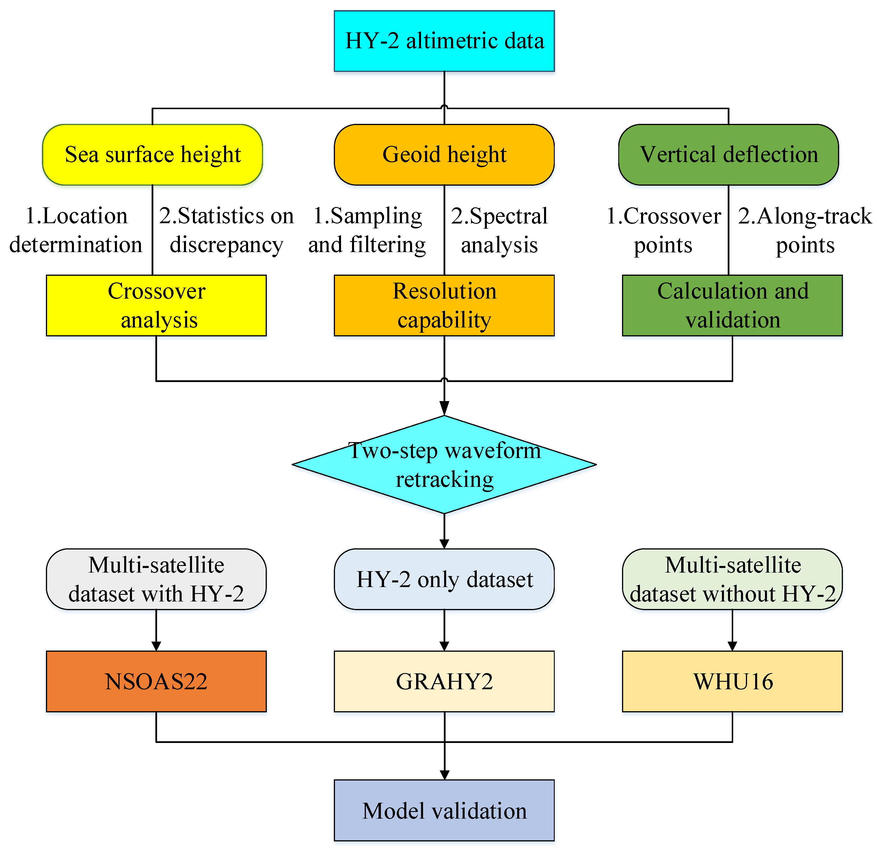
Figure 1.
Flowchart for evaluating HY-2 altimetric data’s performance in marine gravity research.
Figure 1.
Flowchart for evaluating HY-2 altimetric data’s performance in marine gravity research.
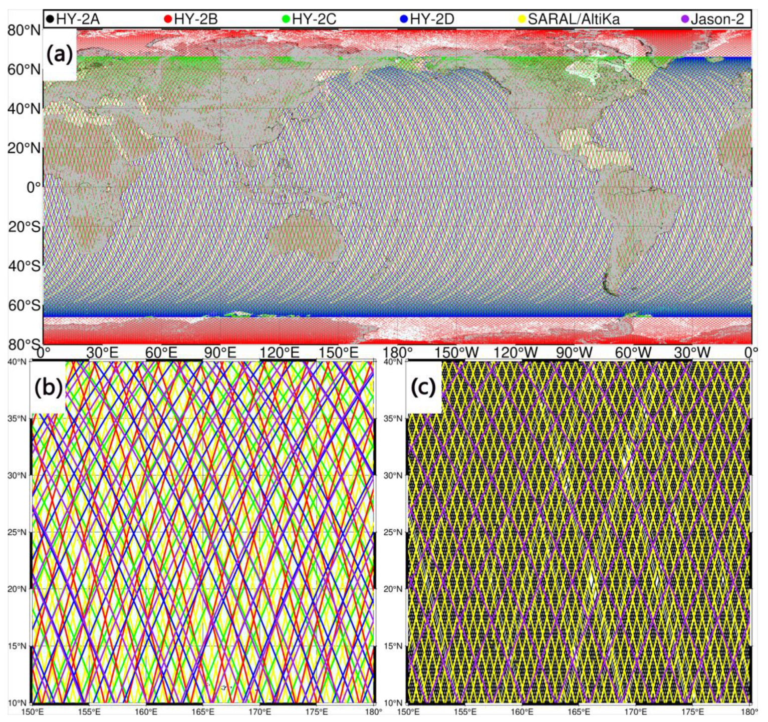
Figure 2.
Global distribution of HY-2 altimetry data and magnification in a 30° × 30° region (Region 1, North Pacific; (a): global distribution of one complete ERM cycle from HY-2B (red), HY-2C (green) and HY-2D (blue); (b): regional distribution of one complete ERM cycle from HY-2B (red), HY-2C (green), HY-2D (blue), SARAL/AltiKa (yellow) and Jason-2 (purple) in Region 1; (c): regional distribution of one complete GM cycle from HY-2A (black) and one complete ERM cycle from SARAL/AltiKa (yellow) and Jason-2 (purple) in Region 1).
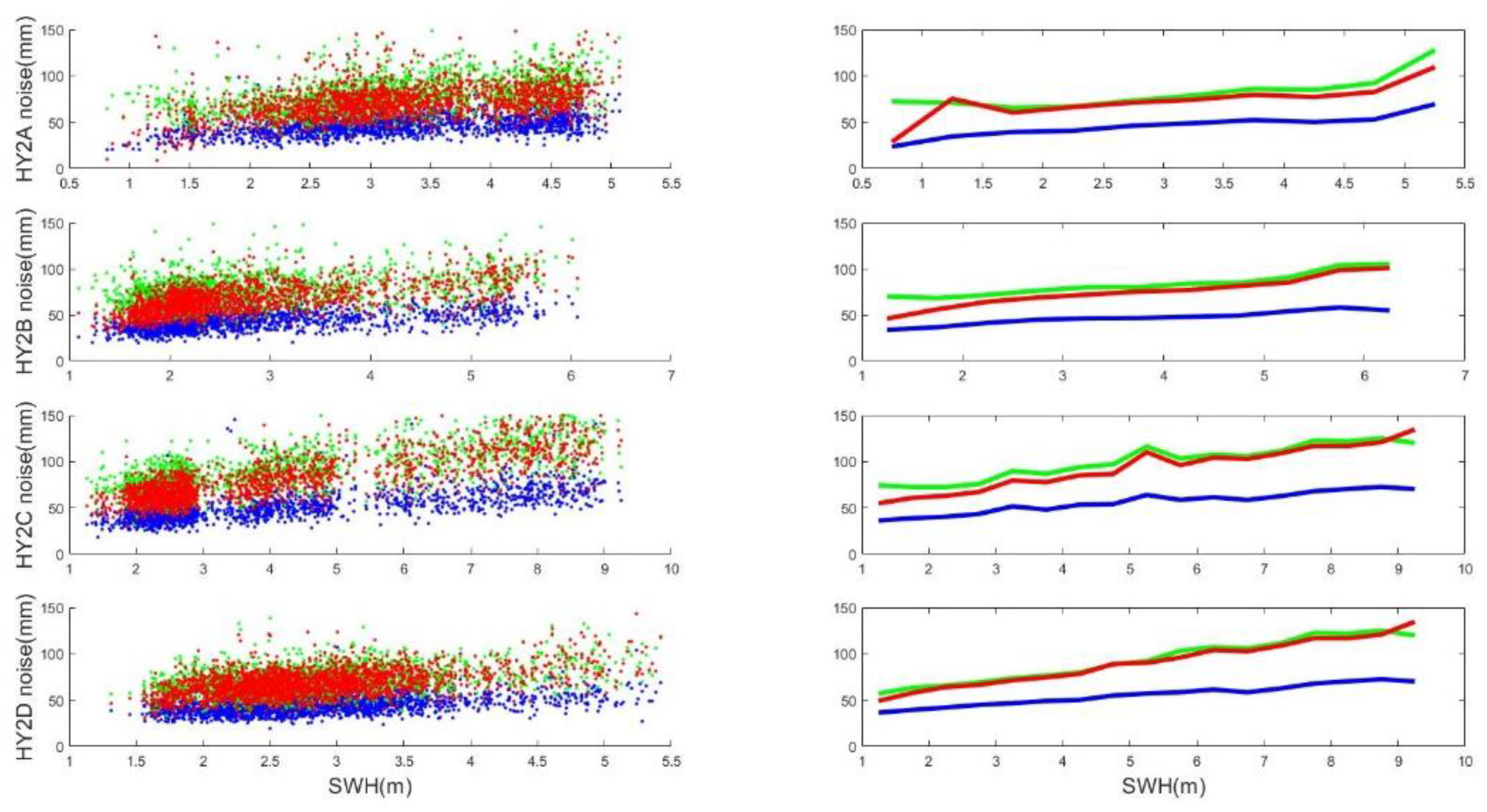
Figure 3.
Standard deviation of retracked height with respect to EGM2008 for HY-2 sample passes. Left figures: statistics for individual points. Right figures: medians over 0.5 m SWH intervals (red: height from sensor geophysical data record; green: height from first step of two-pass retracking; blue: height from second step of two-pass retracking).
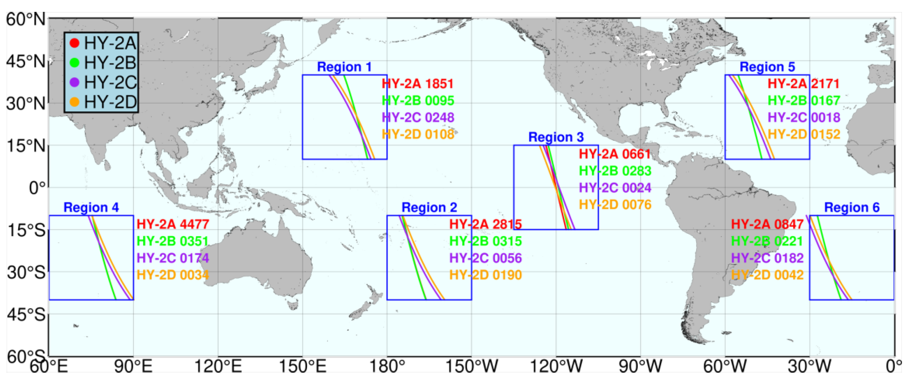
Figure 4.
Selected study regions and sample pass groups of HY-2A, HY-2B, HY-2C and HY-2D with similar spatial distribution (Region 1, North Pacific; Region 2, South Pacific; Region 3, Mid-Pacific; Region 4, Indian Ocean; Region 5, North Atlantic; Region 6, South Atlantic).
Figure 4.
Selected study regions and sample pass groups of HY-2A, HY-2B, HY-2C and HY-2D with similar spatial distribution (Region 1, North Pacific; Region 2, South Pacific; Region 3, Mid-Pacific; Region 4, Indian Ocean; Region 5, North Atlantic; Region 6, South Atlantic).
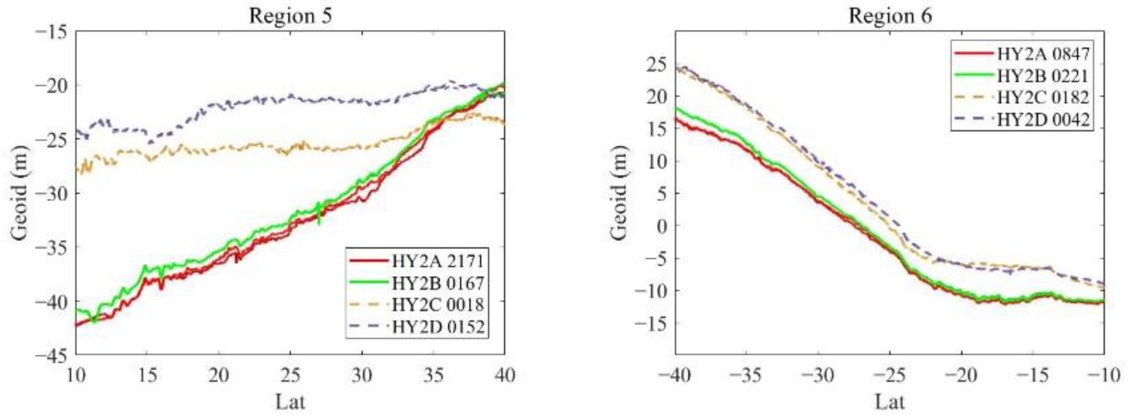
Figure 5.
Variation trend of geoid heights along sample data sequences for HY-2A, HY-2B, HY-2C and HY-2D: Region 1, North Pacific; Region 2, South Pacific; Region 3, Mid-Pacific; Region 4, Indian Ocean; Region 5, North Atlantic; Region 6, South Atlantic.
Figure 5.
Variation trend of geoid heights along sample data sequences for HY-2A, HY-2B, HY-2C and HY-2D: Region 1, North Pacific; Region 2, South Pacific; Region 3, Mid-Pacific; Region 4, Indian Ocean; Region 5, North Atlantic; Region 6, South Atlantic.
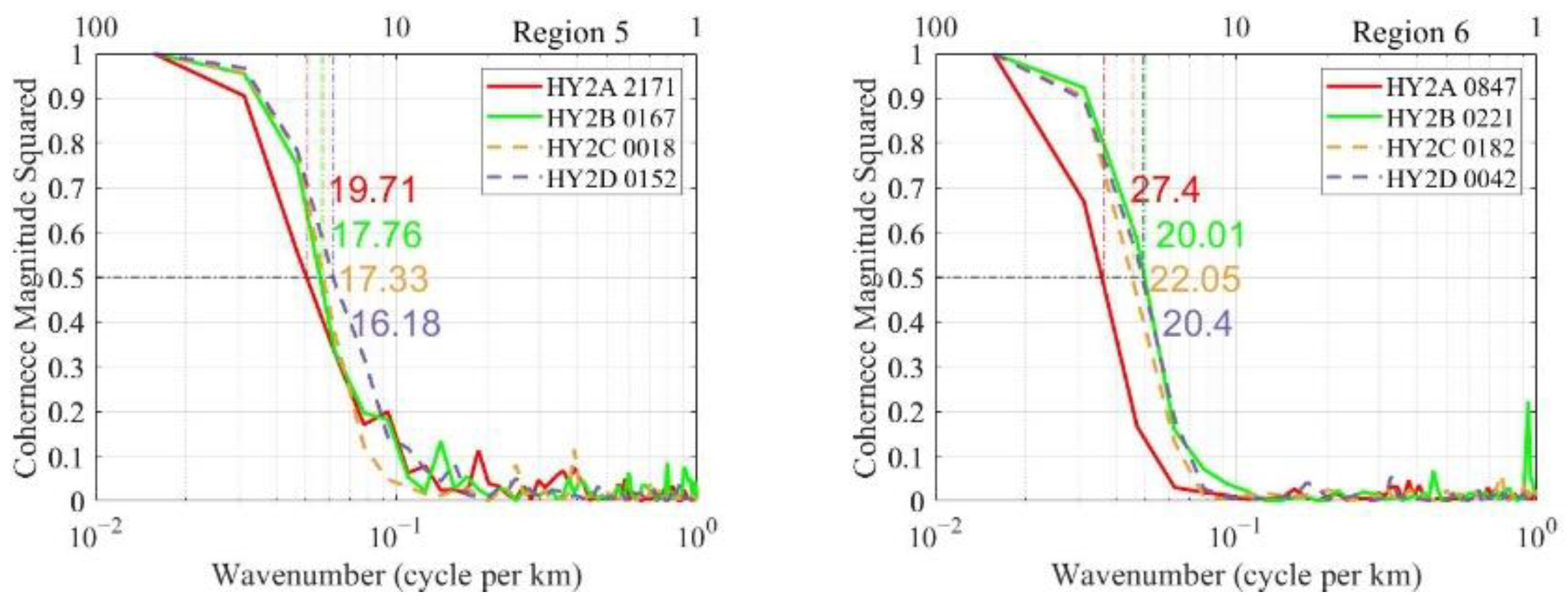
Figure 6.
Coherence map and deduced resolution capabilities of repeat track data sequences for HY-2A, HY-2B, HY-2C and HY-2D over study regions: Region 1, North Pacific; Region 2, South Pacific; Region 3, Mid-Pacific; Region 4, Indian Ocean; Region 5, North Atlantic; Region 6, South Atlantic.
Figure 6.
Coherence map and deduced resolution capabilities of repeat track data sequences for HY-2A, HY-2B, HY-2C and HY-2D over study regions: Region 1, North Pacific; Region 2, South Pacific; Region 3, Mid-Pacific; Region 4, Indian Ocean; Region 5, North Atlantic; Region 6, South Atlantic.
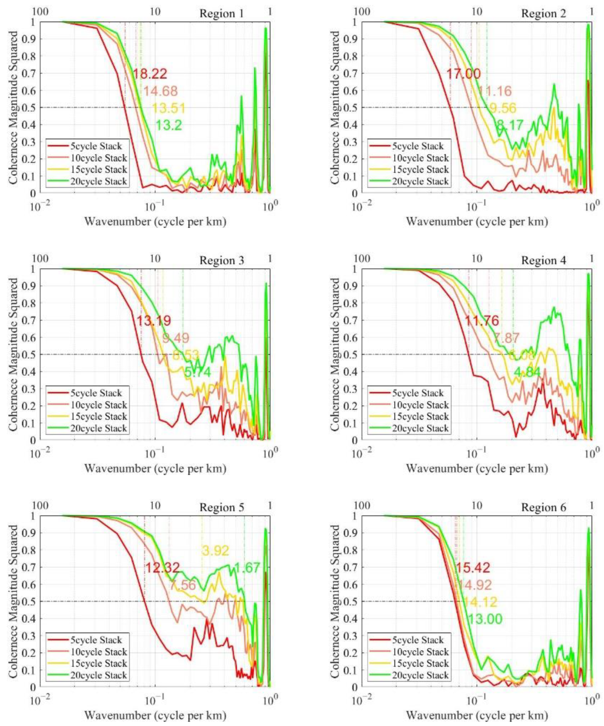
Figure 7.
Coherence map and deduced resolution capabilities of HY-2B repeat track data sequences after stacking 5, 10, 15, 20 cycles’ data: Region 1, North Pacific; Region 2, South Pacific; Region 3, Mid-Pacific; Region 4, Indian Ocean; Region 5, North Atlantic; Region 6, South Atlantic.
Figure 7.
Coherence map and deduced resolution capabilities of HY-2B repeat track data sequences after stacking 5, 10, 15, 20 cycles’ data: Region 1, North Pacific; Region 2, South Pacific; Region 3, Mid-Pacific; Region 4, Indian Ocean; Region 5, North Atlantic; Region 6, South Atlantic.
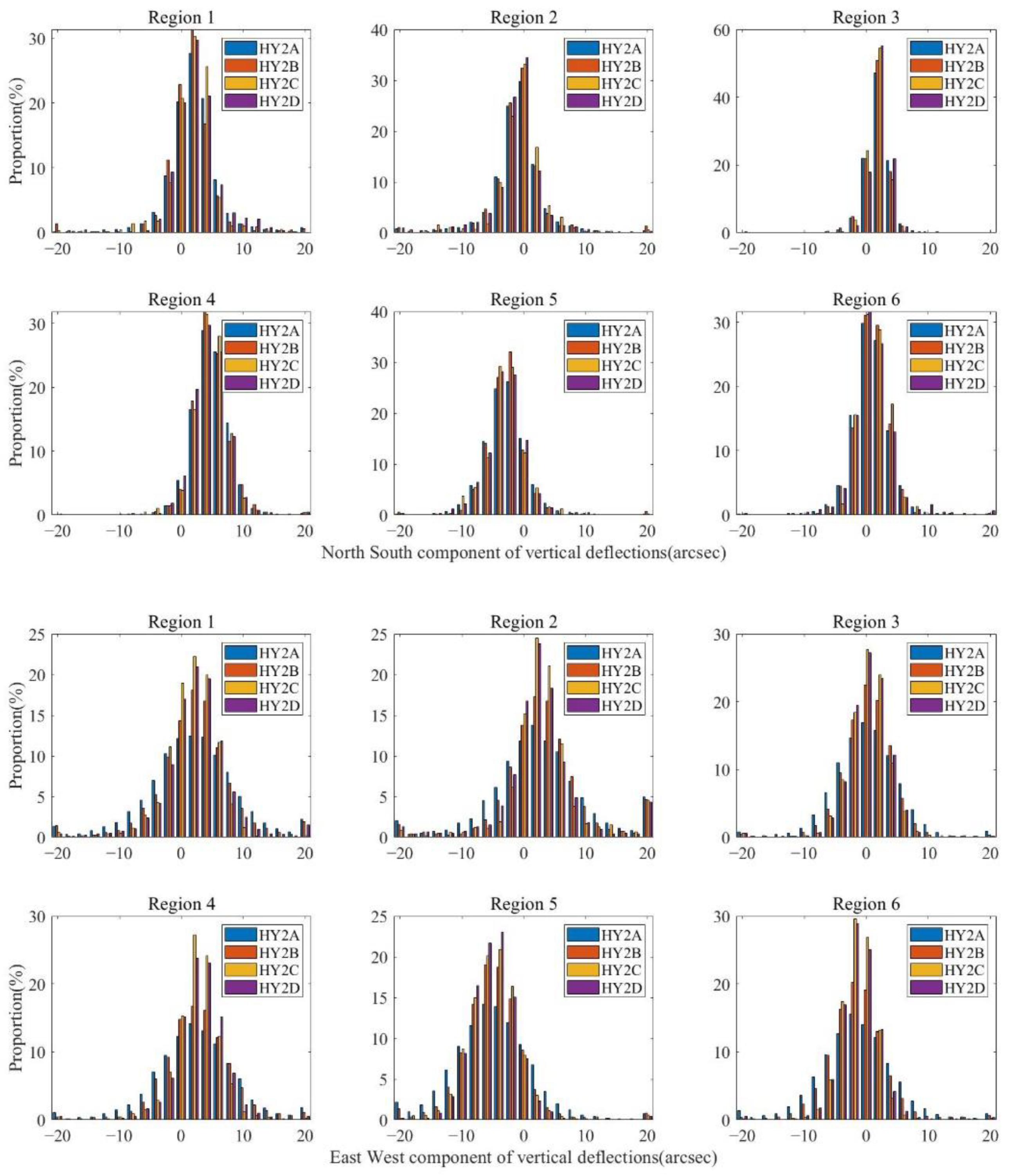
Figure 8.
Distributional proportion of HY-2 directional components of vertical deflection over study regions: Region 1, North Pacific; Region 2, South Pacific; Region 3, Mid-Pacific; Region 4, Indian Ocean; Region 5, North Atlantic; Region 6, South Atlantic.
Figure 8.
Distributional proportion of HY-2 directional components of vertical deflection over study regions: Region 1, North Pacific; Region 2, South Pacific; Region 3, Mid-Pacific; Region 4, Indian Ocean; Region 5, North Atlantic; Region 6, South Atlantic.
Figure 9.
Distributional proportion of discrepancies between HY-2 directional components and XGM2019 model: Region 1, North Pacific; Region 2, South Pacific; Region 3, Mid-Pacific; Region 4, Indian Ocean; Region 5, North Atlantic; Region 6, South Atlantic.
Figure 9.
Distributional proportion of discrepancies between HY-2 directional components and XGM2019 model: Region 1, North Pacific; Region 2, South Pacific; Region 3, Mid-Pacific; Region 4, Indian Ocean; Region 5, North Atlantic; Region 6, South Atlantic.
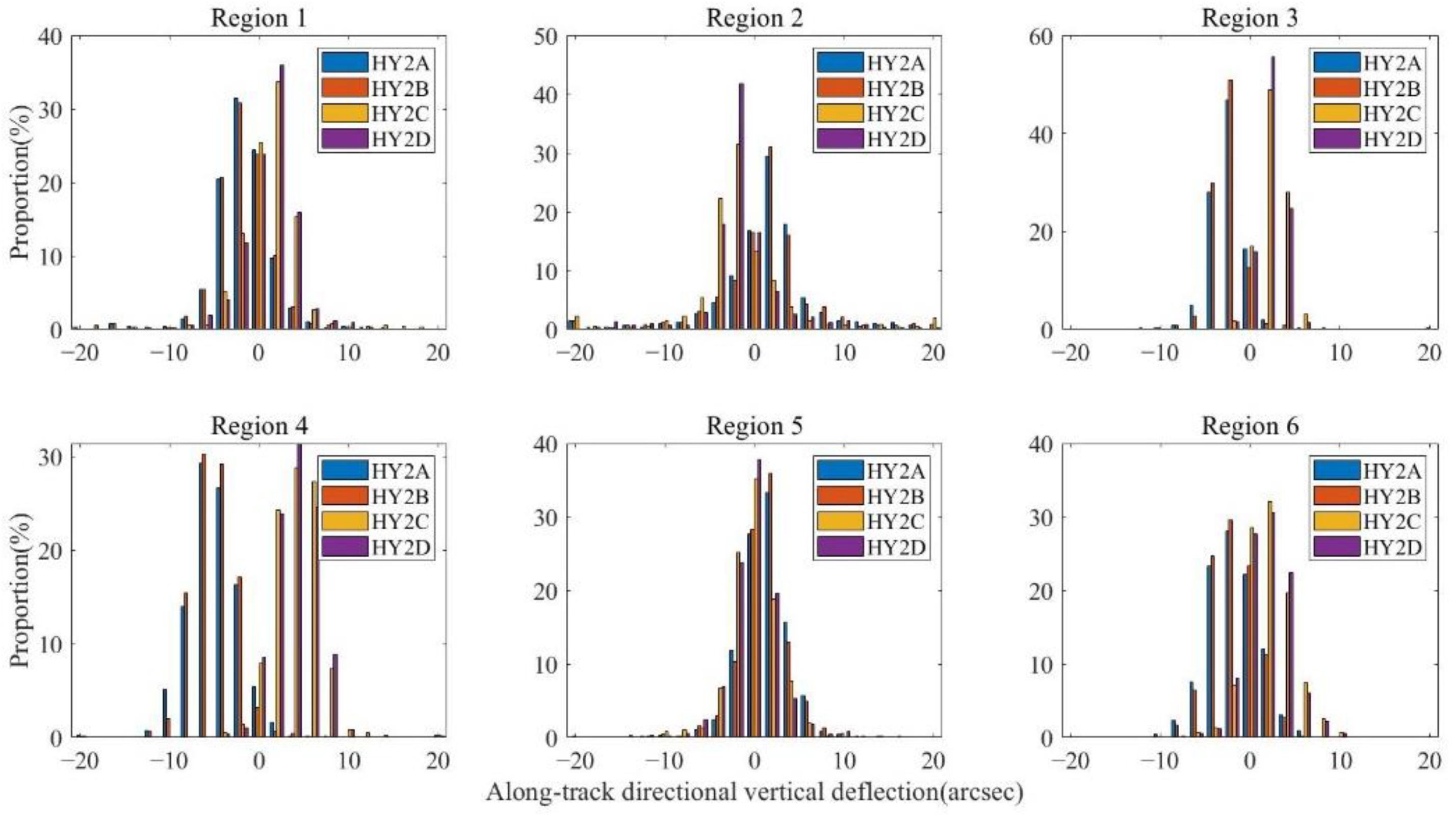
Figure 10.
Distributional proportion of HY-2 along-track vertical deflections over study regions (unit: arcsec): Region 1, North Pacific; Region 2, South Pacific; Region 3, Mid-Pacific; Region 4, Indian Ocean; Region 5, North Atlantic; Region 6, South Atlantic.
Figure 10.
Distributional proportion of HY-2 along-track vertical deflections over study regions (unit: arcsec): Region 1, North Pacific; Region 2, South Pacific; Region 3, Mid-Pacific; Region 4, Indian Ocean; Region 5, North Atlantic; Region 6, South Atlantic.
Figure 11.
Distributional proportion of discrepancies between HY-2 along-track vertical deflections and XGM2019 model (unit: arcsec): Region 1, North Pacific; Region 2, South Pacific; Region 3, Mid-Pacific; Region 4, Indian Ocean; Region 5, North Atlantic; Region 6, South Atlantic.
Figure 11.
Distributional proportion of discrepancies between HY-2 along-track vertical deflections and XGM2019 model (unit: arcsec): Region 1, North Pacific; Region 2, South Pacific; Region 3, Mid-Pacific; Region 4, Indian Ocean; Region 5, North Atlantic; Region 6, South Atlantic.
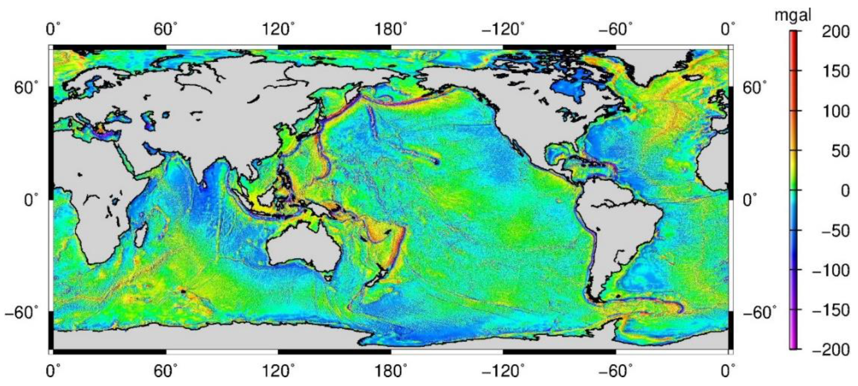
Figure 12.
Global gravity anomaly model NSOAS22.
Figure 12.
Global gravity anomaly model NSOAS22.
Figure 13.
Residual gravity anomaly of GRAHY2, WHU16 and NSOAS22 models in the six study regions and difference between NSOAS22 and WHU16 (the lowercase letters (a–d) represent GRAHY2, WHU16, NSOAS22 and difference between NSOAS22 and WHU16; the Arabic numbers (1–6) represent the study regions).
Figure 13.
Residual gravity anomaly of GRAHY2, WHU16 and NSOAS22 models in the six study regions and difference between NSOAS22 and WHU16 (the lowercase letters (a–d) represent GRAHY2, WHU16, NSOAS22 and difference between NSOAS22 and WHU16; the Arabic numbers (1–6) represent the study regions).
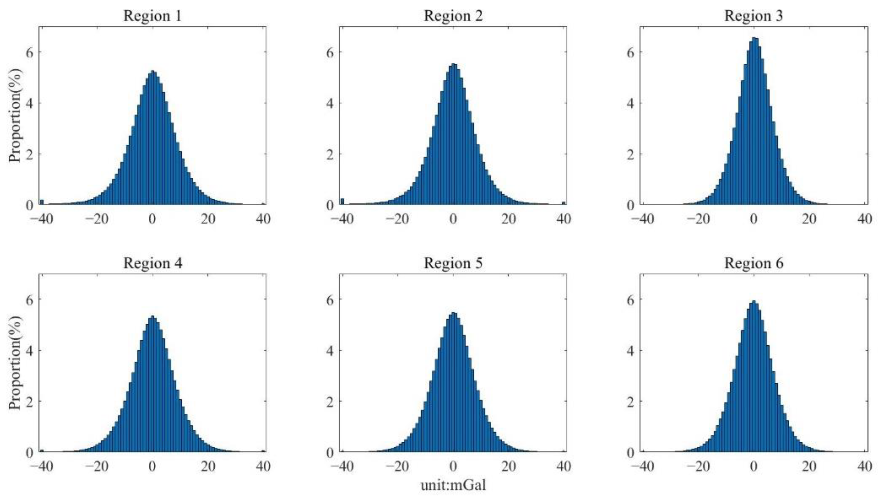
Figure 14.
Histogram of the differences between NSOAS22 and WHU16 in the six study regions: Region 1, North Pacific; Region 2, South Pacific; Region 3, Mid-Pacific; Region 4, Indian Ocean; Region 5, North Atlantic; Region 6, South Atlantic.
Figure 14.
Histogram of the differences between NSOAS22 and WHU16 in the six study regions: Region 1, North Pacific; Region 2, South Pacific; Region 3, Mid-Pacific; Region 4, Indian Ocean; Region 5, North Atlantic; Region 6, South Atlantic.
Table 1.
List of parameters used to estimate the SSH for HY-2 series missions (ECMWF, NCEP and GIM are the European Centre for Medium-Range Weather Forecasts, National Centers for Environmental Prediction, and Global Ionospheric Map).
Table 1.
List of parameters used to estimate the SSH for HY-2 series missions (ECMWF, NCEP and GIM are the European Centre for Medium-Range Weather Forecasts, National Centers for Environmental Prediction, and Global Ionospheric Map).
| Contrastive Parameters | HY-2A | HY-2B, HY-2C and HY-2D |
|---|
| Dry troposphere correction | ECMWF | NCEP |
| Wet troposphere correction | ECMWF | NCEP |
| Ionospheric correction | Dual-frequency | GIM |
| Sea state bias | NSOAS empirical solution | NSOAS empirical solution |
| Ocean tide | GOT00.2 | GOT4.10c |
| Solid earth tide | Cartwright and Tayler tables | Cartwright and Tayler tables |
| Pole tide | Wahr [25] | Wahr [25] |
| Inverted barometer correction | NCEP | NCEP |
Table 2.
Statistics of crossover discrepancy with different time limits for four HY-2 missions: Region 1, North Pacific; Region 2, South Pacific; Region 3, Mid-Pacific; Region 4, Indian Ocean; Region 5, North Atlantic; Region 6, South Atlantic.
Table 2.
Statistics of crossover discrepancy with different time limits for four HY-2 missions: Region 1, North Pacific; Region 2, South Pacific; Region 3, Mid-Pacific; Region 4, Indian Ocean; Region 5, North Atlantic; Region 6, South Atlantic.
| Experimental Region | Time Limit | HY-2A | HY-2B | HY-2C | HY-2D |
|---|
| Num | SD (m) | Num | SD (m) | Num | SD (m) | Num | SD (m) |
|---|
| 1 | <168 days | 8370 | 0.1942 | 8564 | 0.1935 | 7413 | 0.1482 | 7566 | 0.1352 |
| <14 days | 1314 | 0.1289 | 2024 | 0.1339 | 2369 | 0.1136 | 2432 | 0.1034 |
| <5 days | 463 | 0.1060 | 812 | 0.1134 | 901 | 0.0990 | 920 | 0.0953 |
| <1 day | 166 | 0.0666 | 241 | 0.0910 | 256 | 0.0726 | 264 | 0.0599 |
| 2 | <168 days | 8315 | 0.1679 | 8492 | 0.1082 | 7418 | 0.1183 | 7195 | 0.1331 |
| <14 days | 1324 | 0.1506 | 2010 | 0.0900 | 2390 | 0.1091 | 2309 | 0.1102 |
| <5 days | 472 | 0.1214 | 807 | 0.0855 | 905 | 0.0945 | 869 | 0.1036 |
| <1 day | 168 | 0.0823 | 236 | 0.0559 | 255 | 0.0793 | 243 | 0.0621 |
| 3 | <168 days | 7286 | 0.1236 | 7695 | 0.1154 | 5608 | 0.1071 | 5647 | 0.1220 |
| <14 days | 1216 | 0.0936 | 1821 | 0.0875 | 1760 | 0.0883 | 1772 | 0.1064 |
| <5 days | 481 | 0.0778 | 705 | 0.0877 | 682 | 0.0831 | 687 | 0.0993 |
| <1 day | — | — | — | — | 173 | 0.0697 | 175 | 0.0640 |
| 4 | <168 days | 8055 | 0.1810 | 8457 | 0.1641 | 7712 | 0.1386 | 7461 | 0.1368 |
| <14 days | 1271 | 0.1365 | 2008 | 0.1273 | 2482 | 0.1153 | 2407 | 0.1036 |
| <5 days | 452 | 0.1176 | 810 | 0.1202 | 941 | 0.1033 | 911 | 0.0889 |
| <1 day | 154 | 0.0929 | 238 | 0.0538 | 260 | 0.0755 | 261 | 0.0745 |
| 5 | <168 days | 8215 | 0.1913 | 8741 | 0.1516 | 7769 | 0.1346 | 7836 | 0.1311 |
| <14 days | 1326 | 0.1628 | 2074 | 0.1074 | 2490 | 0.1083 | 2508 | 0.1161 |
| <5 days | 471 | 0.1052 | 830 | 0.0921 | 941 | 0.0912 | 944 | 0.1034 |
| <1 day | 167 | 0.0681 | 242 | 0.0664 | 259 | 0.0760 | 269 | 0.0610 |
| 6 | <168 days | 8150 | 0.1446 | 8611 | 0.0903 | 7674 | 0.0973 | 7745 | 0.1099 |
| <14 days | 1292 | 0.1248 | 2037 | 0.0822 | 2458 | 0.0884 | 2491 | 0.0966 |
| <5 days | 455 | 0.1352 | 820 | 0.0706 | 928 | 0.0855 | 944 | 0.0862 |
| <1 day | 159 | 0.1205 | 240 | 0.0507 | 259 | 0.0666 | 269 | 0.0577 |
Table 3.
Summary of information for sample data sequences in 6 research regions: Region 1, North Pacific; Region 2, South Pacific; Region 3, Mid-Pacific; Region 4, Indian Ocean; Region 5, North Atlantic; Region 6, South Atlantic.
Table 3.
Summary of information for sample data sequences in 6 research regions: Region 1, North Pacific; Region 2, South Pacific; Region 3, Mid-Pacific; Region 4, Indian Ocean; Region 5, North Atlantic; Region 6, South Atlantic.
| Experimental Region | Satellite | Track Direction | Track Number | Cycle | Date | Data Quantity | Average Distance between Two Cycles |
|---|
| 1 | HY-2A | ascending | 1851 | 005 | 2 April | 9285 | 1.101 km |
| 006 | 17 September | 9283 |
| HY-2B | ascending | 0095 | 032 | 10 January | 10,532 | 0.086 km |
| 033 | 24 January | 10,571 |
| HY-2C | descending | 0248 | 019 | 13 March | 11,668 | 0.242 km |
| 020 | 10 April | 11,667 |
| HY-2D | descending | 0108 | 025 | 24 January | 11,633 | 0.156 km |
| 026 | 3 February | 11,676 |
| 2 | HY-2A | ascending | 2815 | 004 | 20 November | 9242 | 0.695 km |
| 006 | 22 October | 9261 |
| HY-2B | ascending | 0315 | 014 | 11 May | 10,504 | 0.195 km |
| 015 | 25 May | 10,522 |
| HY-2C | descending | 0056 | 019 | 24 March | 11,672 | 0.276 km |
| 020 | 3 April | 11,644 |
| HY-2D | descending | 0190 | 026 | 6 February | 11,672 | 0.025 km |
| 028 | 26 February | 11,676 |
| 3 | HY-2A | ascending | 0661 | 005 | 18 February | 9254 | 0.131 km |
| 006 | 5 August | 9251 |
| HY-2B | ascending | 0283 | 017 | 21 June | 10,479 | 0.230 km |
| 019 | 19 July | 10,477 |
| HY-2C | descending | 0024 | 011 | 2 January | 11,337 | 0.011 km |
| 012 | 12 January | 11,349 |
| HY-2D | descending | 0076 | 028 | 22 February | 11,364 | 0.249 km |
| 032 | 2 April | 11,318 |
| 4 | HY-2A | ascending | 4477 | 003 | 4 August | 9218 | 0.113 km |
| 005 | 6 July | 9249 |
| HY-2B | ascending | 0351 | 019 | 21 July | 10,453 | 0.054 km |
| 020 | 4 August | 10,518 |
| HY-2C | descending | 0174 | 017 | 8 March | 11,636 | 0.159 km |
| 019 | 28 March | 11,637 |
| HY-2D | descending | 0034 | 027 | 10 February | 11,633 | 0.156 km |
| 028 | 20 February | 11,676 |
| 5 | HY-2A | ascending | 2171 | 005 | 13 April | 8689 | 1.369 km |
| 007 | 15 March | 8693 |
| HY-2B | ascending | 0167 | 012 | 7 April | 10,529 | 0.146 km |
| 013 | 21 April | 10,567 |
| HY-2C | descending | 0018 | 015 | 11 February | 11,663 | 0.271 km |
| 016 | 21 February | 11,663 |
| HY-2D | descending | 0152 | 025 | 26 January | 11,661 | 0.160 km |
| 028 | 24 February | 11,674 |
| 6 | HY-2A | ascending | 0847 | 004 | 9 September | 9256 | 0.444 km |
| 006 | 11 August | 9236 |
| HY-2B | ascending | 0221 | 014 | 9 March | 10,524 | 0.084 km |
| 015 | 18 March | 10,520 |
| HY-2C | descending | 0182 | 017 | 9 March | 11,665 | 0.130 km |
| 018 | 18 March | 11,672 |
| HY-2D | descending | 0042 | 027 | 11 February | 11,145 | 0.119 km |
| 028 | 20 February | 11,628 |
Table 4.
Summary of resolution capabilities for HY-2 data sequences: Region 1, North Pacific; Region 2, South Pacific; Region 3, Mid-Pacific; Region 4, Indian Ocean; Region 5, North Atlantic; Region 6, South Atlantic.
Table 4.
Summary of resolution capabilities for HY-2 data sequences: Region 1, North Pacific; Region 2, South Pacific; Region 3, Mid-Pacific; Region 4, Indian Ocean; Region 5, North Atlantic; Region 6, South Atlantic.
| Experimental Region | Satellite | Resolution |
|---|
| 1 | HY-2A | 27.27 km |
| HY-2B | 24.51 km |
| HY-2C | 23.92 km |
| HY-2D | 25.12 km |
| 2 | HY-2A | 23.36 km |
| HY-2B | 22.58 km |
| HY-2C | 17.74 km |
| HY-2D | 19.95 km |
| 3 | HY-2A | 21.03 km |
| HY-2B | 16.44 km |
| HY-2C | 20.09 km |
| HY-2D | 16.71 km |
| 4 | HY-2A | 20.51 km |
| HY-2B | 18.58 km |
| HY-2C | 14.99 km |
| HY-2D | 15.53 km |
| 5 | HY-2A | 19.71 km |
| HY-2B | 17.76 km |
| HY-2C | 17.33 km |
| HY-2D | 16.18 km |
| 6 | HY-2A | 27.40 km |
| HY-2B | 20.01 km |
| HY-2C | 22.05 km |
| HY-2D | 20.40 km |
Table 5.
The average resolution capabilities and improvement effect of HY-2B stacking data.
Table 5.
The average resolution capabilities and improvement effect of HY-2B stacking data.
| HY-2B Stacking Cycles | Resolution of Mean Geoid | Effect of Every Cycle Improving | Improving Percentage |
|---|
| Reference pass | 19.98 km | —— | —— |
| 5 cycles | 14.65 km | 1.332 km/cycle | 26.67% |
| 10 cycles | 10.94 km | 1.004 km/cycle | 45.24% |
| 15 cycles | 9.28 km | 0.713 km/cycle | 53.55% |
| 20 cycles | 7.77 km | 0.610 km/cycle | 61.11% |
Table 6.
Validation for directional components of vertical deflection at crossover points with XGM2019 model (unit: arcsec): Region 1, North Pacific; Region 2, South Pacific; Region 3, Mid-Pacific; Region 4, Indian Ocean; Region 5, North Atlantic; Region 6, South Atlantic.
Table 6.
Validation for directional components of vertical deflection at crossover points with XGM2019 model (unit: arcsec): Region 1, North Pacific; Region 2, South Pacific; Region 3, Mid-Pacific; Region 4, Indian Ocean; Region 5, North Atlantic; Region 6, South Atlantic.
| Experimental Region | HY-2A | HY-2B | HY-2C | HY-2D |
|---|
| NS-SD | EW-SD | NS-SD | EW-SD | NS-SD | EW-SD | NS-SD | EW-SD |
|---|
| 1 | 1.8158 | 5.8641 | 1.8111 | 3.6730 | 1.4160 | 2.4234 | 1.4950 | 2.8535 |
| 2 | 1.8060 | 6.0823 | 1.3033 | 3.8435 | 1.3650 | 2.6606 | 1.4224 | 2.6351 |
| 3 | 1.2695 | 4.8377 | 0.9614 | 3.0489 | 0.9961 | 2.3396 | 0.9435 | 2.1194 |
| 4 | 1.8012 | 6.0917 | 1.4912 | 4.3776 | 1.5263 | 2.3788 | 1.3558 | 2.4246 |
| 5 | 1.9329 | 5.8834 | 1.5815 | 3.3820 | 1.7654 | 2.4545 | 1.5086 | 2.2948 |
| 6 | 1.8720 | 5.6527 | 1.4436 | 3.7008 | 1.5509 | 2.1746 | 1.6584 | 2.1735 |
| Average | 1.7495 | 5.7353 | 1.4320 | 3.6709 | 1.4366 | 2.4052 | 1.3972 | 2.4168 |
Table 7.
Comparison of determined along-track vertical deflections with XGM2019 for HY-2 missions (unit: arcsec): Region 1, North Pacific; Region 2, South Pacific; Region 3, Mid-Pacific; Region 4, Indian Ocean; Region 5, North Atlantic; Region 6, South Atlantic.
Table 7.
Comparison of determined along-track vertical deflections with XGM2019 for HY-2 missions (unit: arcsec): Region 1, North Pacific; Region 2, South Pacific; Region 3, Mid-Pacific; Region 4, Indian Ocean; Region 5, North Atlantic; Region 6, South Atlantic.
| Experimental Region | HY-2A | HY-2B | HY-2C | HY-2D |
|---|
| Num | SD | Num | SD | Num | SD | Num | SD |
|---|
| 1 | 1057 | 1.4130 | 1058 | 1.3100 | 1167 | 1.0749 | 1166 | 1.2805 |
| 2 | 1060 | 1.4783 | 1060 | 1.0544 | 1168 | 1.0571 | 1167 | 0.9400 |
| 3 | 1054 | 1.2890 | 1054 | 0.8987 | 1135 | 1.0829 | 1137 | 0.8626 |
| 4 | 1059 | 1.7919 | 1059 | 1.1186 | 1168 | 1.1093 | 1161 | 1.0600 |
| 5 | 994 | 1.4002 | 1056 | 0.9773 | 1166 | 1.1223 | 1167 | 0.9631 |
| 6 | 1060 | 1.3742 | 1060 | 0.9170 | 1051 | 1.0810 | 1167 | 0.9359 |
| Average | 6284 | 1.4578 | 6347 | 1.0460 | 6855 | 1.0879 | 6965 | 1.0070 |
Table 8.
Statistics of the differences between NSOAS22 and WHU16 in the six study regions (unit: mGal): Region 1, North Pacific; Region 2, South Pacific; Region 3, Mid-Pacific; Region 4, Indian Ocean; Region 5, North Atlantic; Region 6, South Atlantic.
Table 8.
Statistics of the differences between NSOAS22 and WHU16 in the six study regions (unit: mGal): Region 1, North Pacific; Region 2, South Pacific; Region 3, Mid-Pacific; Region 4, Indian Ocean; Region 5, North Atlantic; Region 6, South Atlantic.
| NSOAS22-WHU16 | Region 1 | Region 2 | Region 3 | Region 4 | Region 5 | Region 6 |
|---|
| Max | 89.0 | 180.4 | 74.6 | 109.4 | 91.0 | 120.0 |
| Min | −150.6 | −209.4 | −93.2 | −95.2 | −99.2 | −138.8 |
| Mean | −0.056 | 0.017 | 0.235 | 0.067 | 0.082 | −0.102 |
| SD | 9.092 | 9.068 | 6.865 | 8.625 | 8.192 | 7.644 |
Table 9.
Statistics of difference between NSOAS22, DTU21 and SS V31.1 (unit: mGal): Region 1, North Pacific; Region 2, South Pacific; Region 3, Mid-Pacific; Region 4, Indian Ocean; Region 5, North Atlantic; Region 6, South Atlantic.
Table 9.
Statistics of difference between NSOAS22, DTU21 and SS V31.1 (unit: mGal): Region 1, North Pacific; Region 2, South Pacific; Region 3, Mid-Pacific; Region 4, Indian Ocean; Region 5, North Atlantic; Region 6, South Atlantic.
| SD(Model) | Region 1 | Region 2 | Region 3 | Region 4 | Region 5 | Region 6 |
|---|
| SD (DTU21-NSOAS22) | 2.1984 | 2.1382 | 1.2778 | 1.8634 | 1.7846 | 1.7260 |
| SD (V31.1-NSOAS22) | 2.2945 | 2.2386 | 1.4460 | 1.9923 | 1.8450 | 1.7619 |
| SD (V31.1-DTU21) | 1.2943 | 1.4832 | 1.1498 | 1.3503 | 1.2564 | 1.1988 |
Table 10.
Statistics of difference between shipborne measurements and typical gravity models (unit: mGal): Region 1, North Pacific; Region 2, South Pacific; Region 3, Mid-Pacific; Region 4, Indian Ocean; Region 5, North Atlantic; Region 6, South Atlantic. (The upper table shows the original statistics, while the lower table shows the accuracy results after a gross error elimination of shipborne measurements.).
| Experimental Region | Ship Num | EGM2008 | V31.1 | DTU21 | NSOAS22 | WHU16 | GRAHY-2 |
|---|
| Comparison with original NGDC shipborne data |
| 1 | 154307 | 8.9969 | 8.4055 | 8.4498 | 8.6485 | 8.7617 | 9.5523 |
| 2 | 223215 | 6.7261 | 6.1551 | 6.0829 | 6.4873 | 6.4206 | 7.9747 |
| 3 | 183428 | 7.0148 | 6.5585 | 6.5938 | 6.6597 | 6.6070 | 7.2480 |
| 4 | 100646 | 5.8313 | 5.2628 | 5.2111 | 5.2717 | 5.3690 | 6.6649 |
| 5 | 77656 | 8.2512 | 8.0527 | 8.0360 | 8.2659 | 8.1806 | 8.8939 |
| 6 | 106374 | 10.0158 | 9.6352 | 9.6369 | 9.9101 | 9.7588 | 10.5042 |
| Average | - | 7.8060 | 7.3449 | 7.3350 | 7.5405 | 7.5162 | 8.4730 |
| Comparison with NGDC shipborne data after a gross error elimination |
| 1 | 130048 | 4.8749 | 4.3306 | 4.3088 | 4.6215 | 4.8435 | 6.0770 |
| 2 | 197434 | 4.8451 | 4.2817 | 4.2640 | 4.3932 | 4.5215 | 6.2772 |
| 3 | 153836 | 4.1413 | 3.9048 | 3.8843 | 3.7998 | 3.9424 | 4.6622 |
| 4 | 68245 | 4.8880 | 4.3855 | 4.3446 | 4.1921 | 4.4148 | 5.8480 |
| 5 | 55325 | 5.5377 | 5.2586 | 5.2472 | 5.2753 | 5.3840 | 6.1715 |
| 6 | 88587 | 4.3236 | 3.6457 | 3.6818 | 4.0168 | 3.8482 | 5.1531 |
| Average | - | 4.7684 | 4.3011 | 4.2884 | 4.3831 | 4.4924 | 5.6981 |


