A Novel Method for Improving Quality of Oblique Incidence Sounding Ionograms Based on Eigenspace-Based Beamforming Technology and Capon High-Resolution Range Profile

Abstract

Ground-based oblique incidence sounding (OIS) is an important means to investigate the ionosphere. As the OIS ionogram is a visual representation of the OIS parameters, such as group distance and maximum usable frequency (MUF), it is of great significance for improving the quality and the range resolution. This will facilitate the automatic interpretation and inversion of OIS ionograms to obtain the fine structure and spatial–temporal evolutions of the ionosphere. In this paper, a novel OIS signal processing scheme is proposed based on the Eigenspace-based (ESB) beamforming technology and Capon high-resolution range profile (HRRP). First, by applying the ESB beamformer to a compact L-shaped antenna array, the energy of the OIS signals received by multiple antennas can be added, while the interference and noise will be suppressed. Subsequently, the Capon HRRP algorithm is used to improve the range resolution. This is achieved due to the slow variation in the characteristics of the ionosphere resulting in good short-term coherence of the narrowband signals. The experimental results show that the two-stage signal-processing method significantly improves the imaging quality of OIS ionograms. In particular, the structure inside the ionosphere and its temporal and spatial evolution can be observed more precisely after the range resolution of the OIS ionogram is improved; therefore, it has great application potential.

1. Introduction

As an important part of the earth’s space environment, the ionosphere can reflect, refract, scatter, and absorb electromagnetic waves. Therefore, the investigation of the ionosphere is of far-reaching significance to space weather and high-frequency radio communications. As is well known, ground-based ionospheric OIS is one of the main ways of sounding the ionosphere, with the advantages of large detecting range, easy networking, and good practicability. It has always been an interesting topic in ionospheric sounding [1,2,3,4]. It should be of great significance to improve the quality and range resolution of OIS ionograms to observe the ionosphere more accurately and finely, such as the internal fine structure of different sporadic E-layers (Es) and the spread F-layers [5,6,7,8].

At present, the methods of improving the quality and range resolution of OIS ionograms can be mainly divided into two categories. (1) Hardware equipment-based, for instance, improving the transmitting power to suppress interference and noise better, as well as increasing the signal bandwidth of the system to improve the range resolution [9,10,11]. However, this means that higher requirements of the hardware and cost will be put forward. At the same time, the larger bandwidth often leads to a poorer sensitivity. It is clearly not particularly suitable for the existing hardware system designed in this paper. (2) Software- and algorithm-based, such as the wavelet image processing method [12], wavelet objective projection filter method [13,14], autoregressive interpolation method [15], and so on. However, due to the large spatial scale, the time-varying spatial distribution, and the internal relative movement of the ionosphere and the resulting complexity, imaging algorithms to improve the range resolution of the OIS ionograms have not been widely considered and applied. In this paper, the Capon HRRP algorithm, which is often used for the detection of aircraft, ships, buildings, and other hard targets [16,17,18,19,20], is first applied to OIS ionogram imaging. Then, the ESB adaptive beamforming technology is also combined to process the OIS signals and reconstruct the ionograms. The implementation process is mainly divided into two steps. First, after the I/Q data of multiple channels is collected by the Wuhan Multi-channel Ionospheric Sounding System (WMISS) [21,22], the ESB adaptive beamforming algorithm is used to synthesize the data of multiple channels, gather the signal energy of each channel and suppress interference and noise. Then, considering that the ionosphere is a soft target that moves slowly, the Capon HRRP algorithm [23,24] is used to improve its range resolution. The experimental results show that the quality of the OIS ionogram is significantly improved. In particular, using the Capon HRRP algorithm, the range resolution is improved, so the fine structure and spatiotemporal changes inside the ionosphere can be observed more precisely. This means that the traditional signal processing technology of OIS still has great room for improvement and application value, which will also be of great significance to the high-precision spatiotemporal observation of the ionosphere in the future.

This paper is roughly divided into seven parts: Section 1. Introduction, which mainly introduces the research background and briefly describes the outline of the problem and our solution; Section 2. WMISS description and introduction; Section 3. Method and data processing flow, in which the. methods of solving the problem and whole data processing flow are described in general; Section 4. ESB algorithm, which describes the principle of ESB adaptive beamforming algorithm; Section 5. High-resolution principle of range profile, which mainly introduces the principle of Capon HRRP algorithm and how to use it in our scheme; Section 6. Results and discussion; Section 7. Conclusions.

2. WMISS Description and Introduction

The original baseband data of OIS comes from WMISS, which is a multifunctional sounding system for the ionosphere. WMISS is mainly composed of three modules: the transmitting module, the receiving module, and the time-frequency synchronization module. The transmitting module is mainly responsible for the transmission of the signal, and the transmitted signal is modulated by pseudo-random two-phase coding. For the OIS of ionosphere, a 16-bit completely complementary code (CCC) is used as the modulation form of the transmitted signal, to make full use of the excellent correlation characteristics of CCC and obtain high gain [21]. The width t_p of each code chip is 25.6 μs, which means that the bandwidth of the transmitted signal is 39.0625 kHz. The transmitting antenna is an inverted V antenna with a frame height of about 8 m, and the transmitting peak power is 200 W.

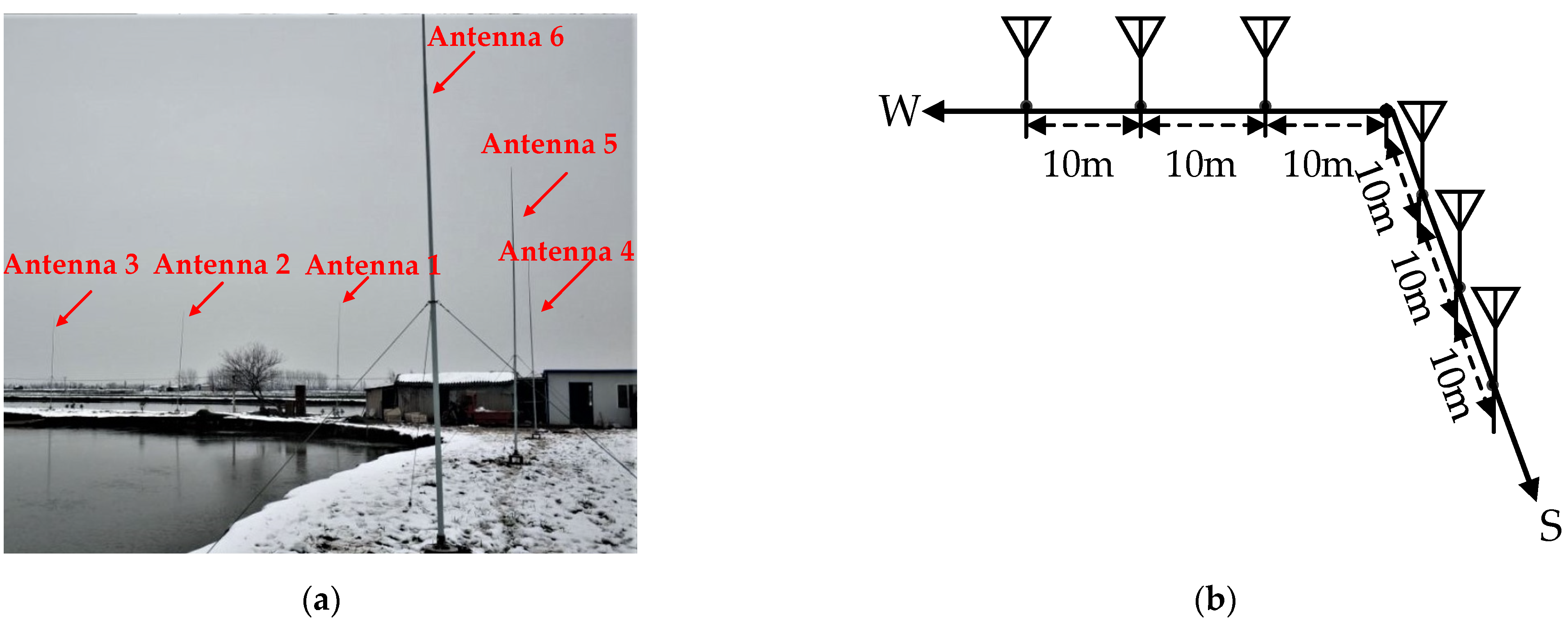
The receiving module is the core of the WMISS system, which is mainly composed of a receiving antenna array and a multi-channel receiver. Its structure diagram is shown in Figure 1. The receiving antenna is a compact “L-shaped” array, composed of 6 monopole antennas with a height of 6 m. 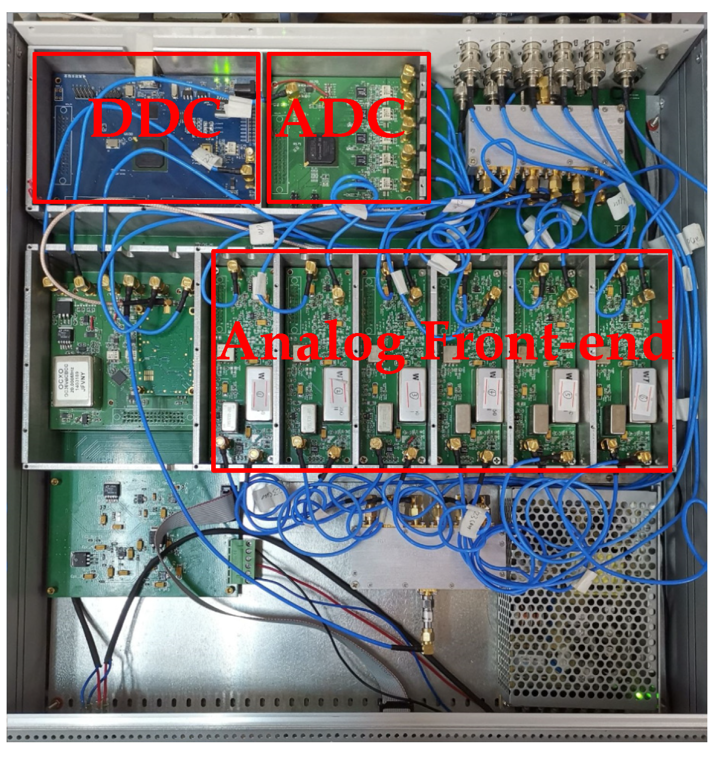The distance between adjacent antennas is 10 m, the actual scene and layout of the site of the “L-shape” array is shown in Figure 2. The received signal of each channel is mixed after preselection filtering to obtain an intermediate frequency signal, which is amplified to an appropriate magnitude after narrowband filtering in the analog front-ends, respectively. Then, it is sampled with high-performance analog/digital (A/D) converters, and the resulting signal is digitally mixed with a quadrature signal generated by a Numerically Controlled Oscillator (NCO), and then filtered by cascaded integrator–comb (CIC) filter and finite impulse response (FIR) filter. The baseband I/Q data stream can be obtained after filtering and decimation. Finally, the baseband I/Q data are uploaded through the USB3.0 transmission bus, and the next step of correlation operation and pulse compression processing is conducted. 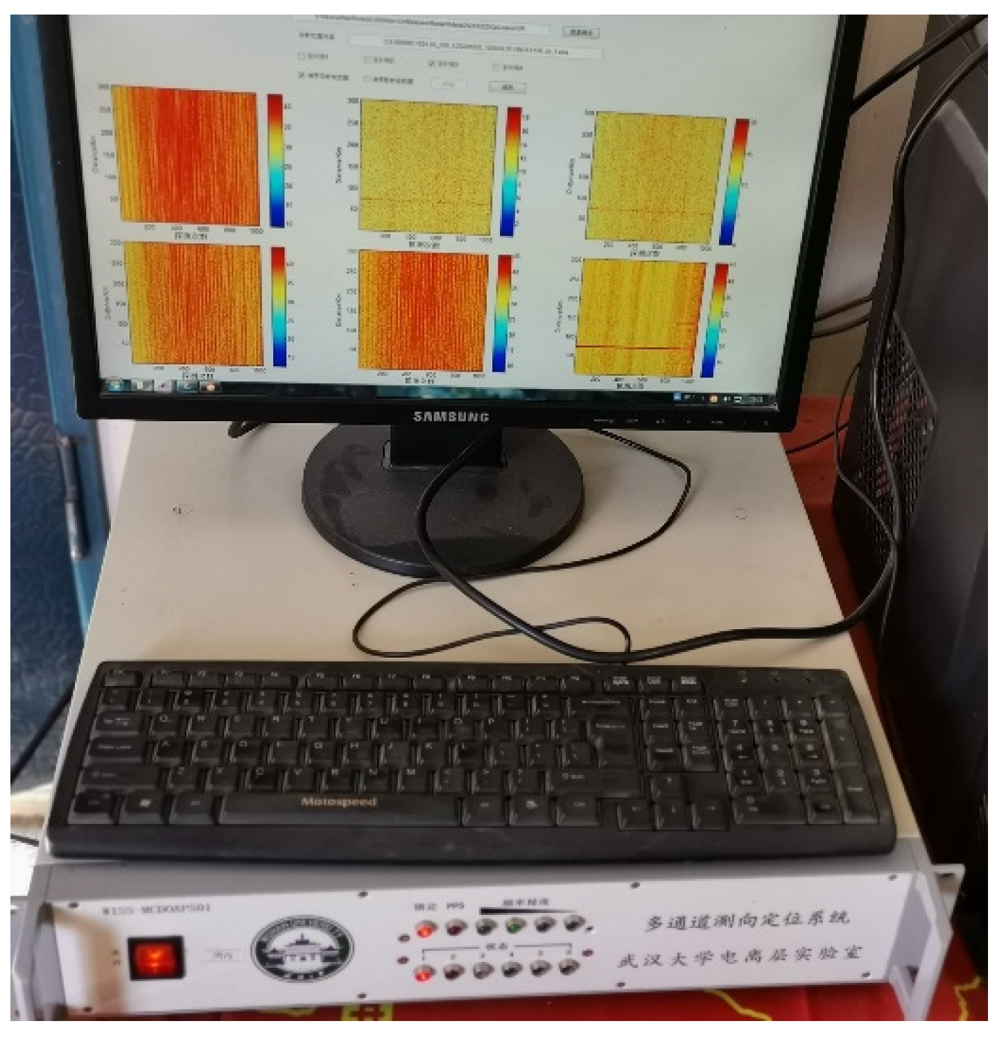The signal processing part of the indoor equipment of the receiving module is shown in Figure 3. Each hardware submodule is independently encapsulated in the aluminum alloy frame, which is conducive to electromagnetic shielding between components. In the multi-channel analog front-end, each analog channel is arranged in parallel, and the adjacent channels are also isolated by an aluminum alloy frame to prevent the mutual crosstalk of electromagnetic signals. Moreover, after the local oscillator source of WMISS is sampled by A/D, it is mixed with the received signal of each channel after a one-to-six power divider (WMISS has six independent channels) to ensure the consistency of the local oscillator source of each channel. At the same time, the connection and internal wiring of each analog channel in the six channels of WMISS use equal-length wires. Finally, in order to ensure that the six channels are phase-coherent, a calibration reference source is introduced, and the amplitude and phase difference between the channels are compared and compensated in the subsequent array signal processing in the upper computer. In addition, the control part of the upper computer is shown in Figure 4, which is mainly responsible for the analysis and storage of data, and downloading instructions and various sounding parameters to the hardware platform of WMISS.

The time–frequency synchronization module provides the operating clock for the entire system and can correct the output frequency of the frequency source in real-time. Furthermore, it ensures the time–frequency synchronization between the transceiver stations.

The main parameters of WMISS are shown in

Table 1. The main parameters of WMISS.

Parameter	Value
Transmitting antenna	Inverted V-shaped
Transmitting power	≤200 W
Receiving antenna	Six monopole antenna
Antenna array shape	L-shaped
Signal coding type	Complete complementary code
Chip width	25.6 μs
Bandwidth	39.0625 kHz
Duty recycle	5%
Sampling number	Fix frequency: 1024/Swept frequency: 32

below.

3. Method and Data Processing Flow

For the scheme designed in this paper, it mainly includes two aspects: Firstly, using ESB adaptive beamforming technology to gather the energy of multiple channels of WMISS, and suppress interference and noise. Through ESB beamforming, the SNR of the echo is significantly improved, and the quality of the OIS ionogram is greatly improved. However, limited by the bandwidth of the short-wave transmitted signal, the original range resolution of the transmitted signal is limited, which limits the further precision observation of the fine structure differences and the temporal–spatial evolution process inside the ionosphere. In view of this situation, combined with the large spatial scale and internal relative movement of the ionosphere, it is a soft target moving slowly. Then, Capon HRRP technology is used to improve the range resolution, which is main innovation of this paper.

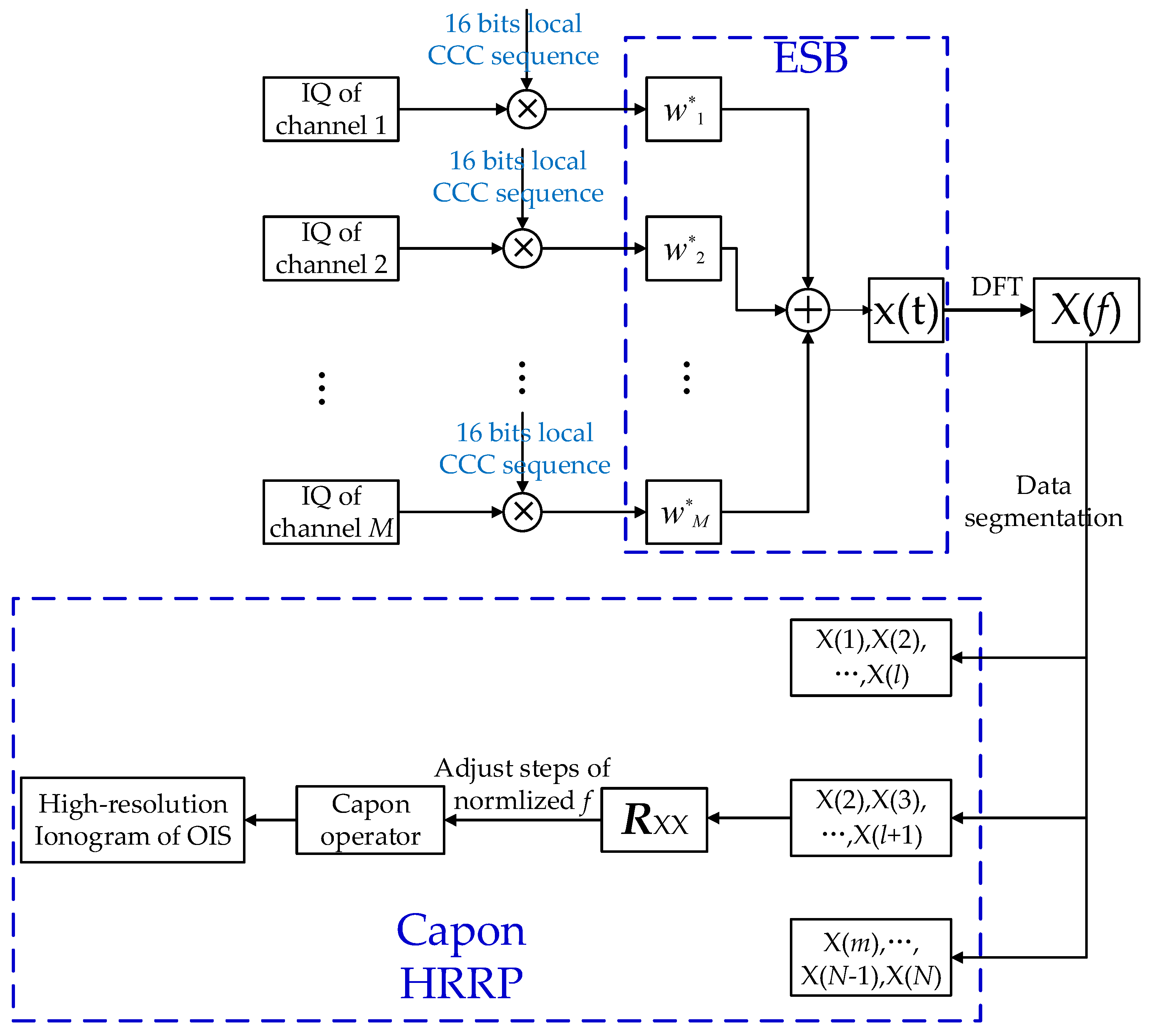
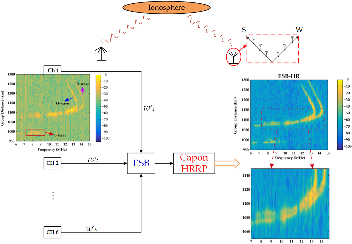
For the scheme proposed in this paper, the general data processing flow is shown in Figure 5: when the OIS baseband I/Q data of each channel are obtained through the WMISS system, it should be cross-correlated with the corresponding local CCC sequence to obtain the imaging results for every range bin. 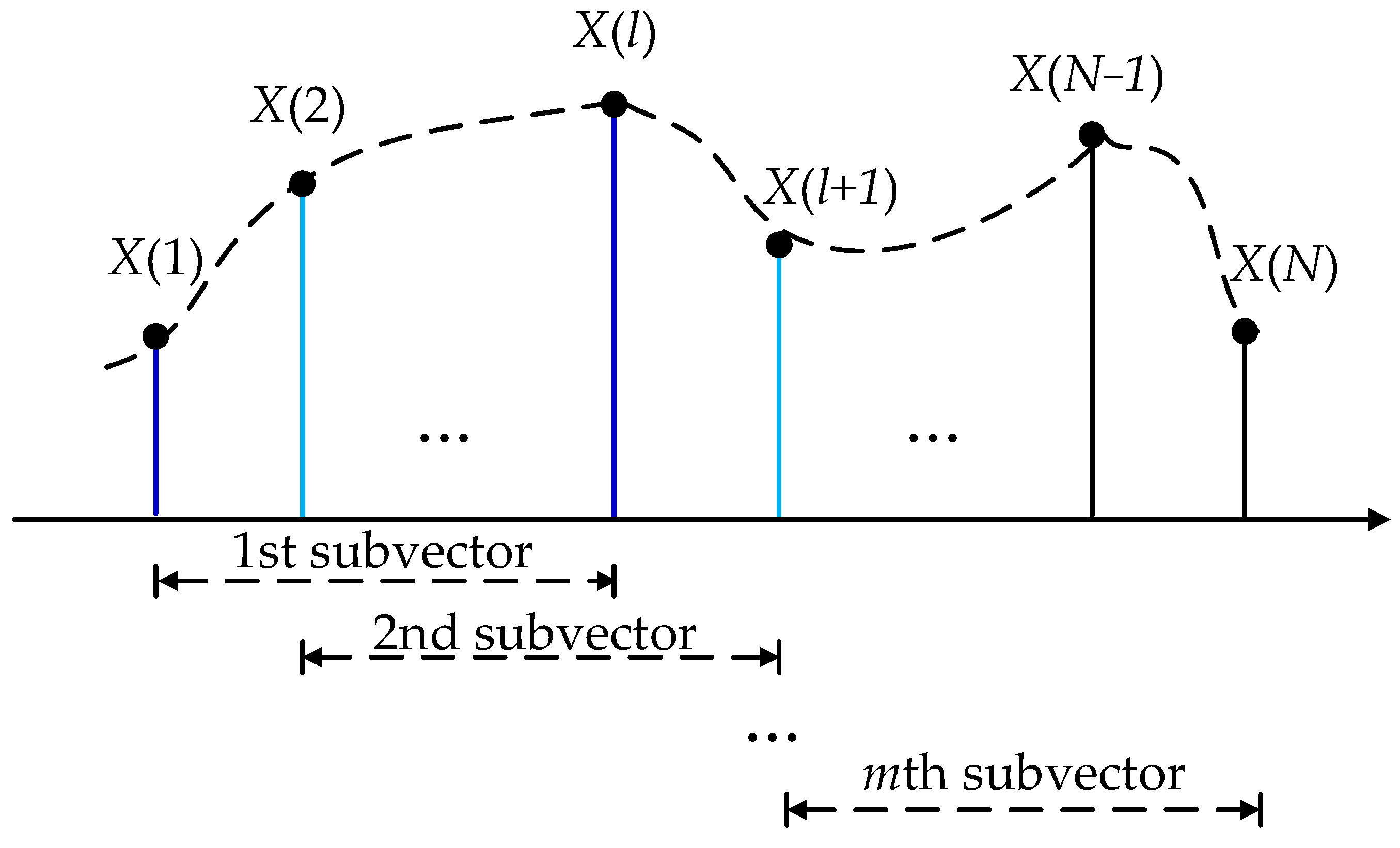Then, taking out the data of the same range bin of M channels, the weighted vector $\mathit{w}$ can be determined by the ESB adaptive beamforming algorithm ((∙)* denotes conjugate in Figure 5). The synthesized signal after weighted summation can be expressed as x(t). Subsequently, discrete Fourier transform (DFT) is performed on the distance dimension of x(t) to obtain the cross energy spectrum X(f). When it is assumed that the echo signal has N range bins, the length of X(f) is N. Through segmenting X(f) into m staggered subvectors of length l, and m + l = N, the covariance matrix Rxx can be constructed. According to the requirements of range resolution, the scanning step should be adjusted and the corresponding steering vector should be calculated. Finally, through using the Capon HRRP algorithm [23,24], the OIS ionogram of the high-resolution range profile can be reconstructed.

The ESB adaptive beamforming technology will be described in the next section, and the Capon HRRP algorithm will be described in detail in Section 5.

4. ESB Adaptive Beamforming Technology

In this paper, ESB beamformer is used in the first step to synthesize the signals of the array optimally, as its excellent processing ability for OIS signal’s synthesis has been proved in the previous research [21]. Its principle can be briefly described as follows.

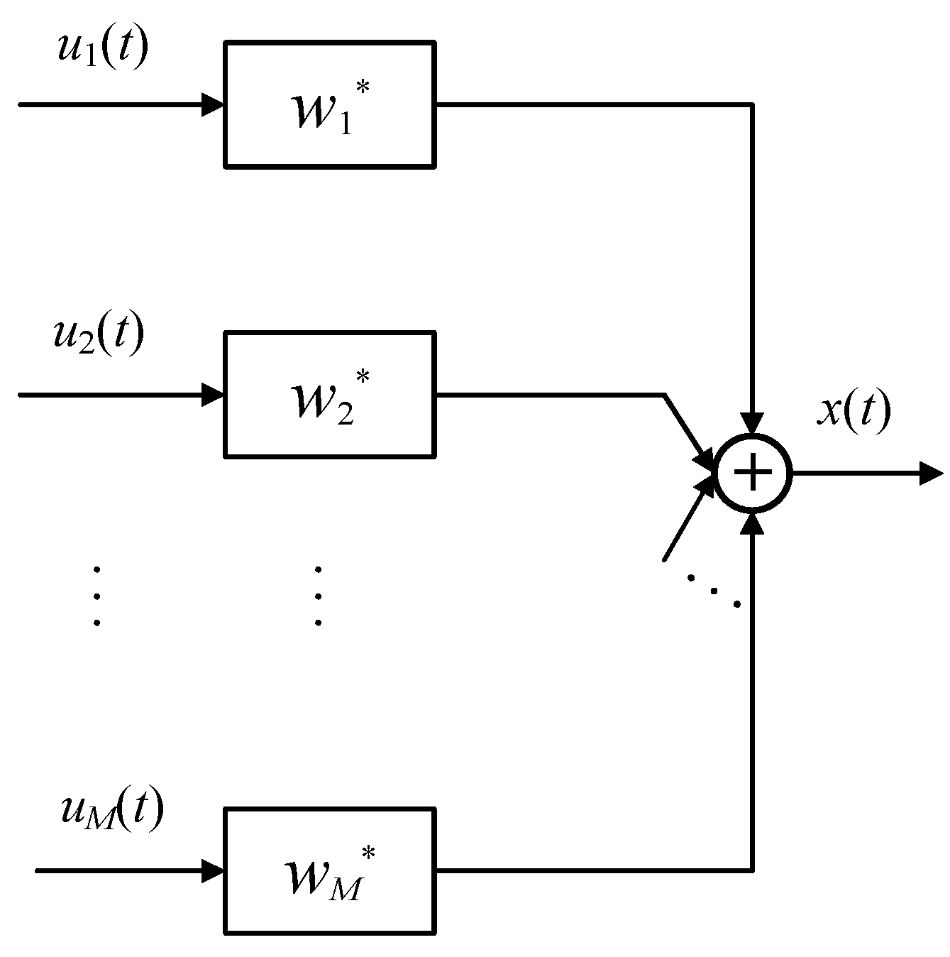
For a general beamformer as shown in Figure 6, assuming there are M array elements, the narrowband beamformer can be written in the form of a vector:

$${\mathit{w}}^H=[w_1^{*},w_2^{*}, \dots ,w_M^{*}]$$

(1)

where $\mathit{w}$ is called the weighted vector. By weighted summation of M array elements, the output of the beamformer is:

$$x(t)={\mathit{w}}^H\mathit{u}(t)$$

(2)

For the most common sampling matrix inversion (SMI) adaptive beamformer, the question of the optimal $\mathit{w}$ can be described as the following constrained minimization problem:

$$\underset{w}{\min } {\mathit{w}}^H{\mathit{R}}_{i+n}\mathit{w} \mathrm{s}.\mathrm{t}.{\mathit{w}}^H{\mathit{a}}_0=1$$

(3)

where R_i+n represents the covariance matrix of interference plus noise, and a₀ represents the steering vector of the desired signal. In practical application, as the received data often contain the desired signal, interference, and noise at the same time, it is impossible to only estimate the covariance matrix of interference and noise R_i+n. Under the condition that the desired signal is guaranteed to be output without distortion, minimizing the variance of the interference and noise output by the beam is equivalent to minimizing the variance of the output received echo. Therefore, the covariance matrix of the desired signal + noise + interference is generally used to replace the covariance matrix of interference + noise [21,25,26]. Then, the weighted vector ${\mathit{w}}_{SMI}$ can be obtained:

$${\mathit{w}}_{SMI}=\frac{{\mathit{R}}_{uu}^{-1}{\mathit{a}}_0}{{\mathit{a}}_0^H{\mathit{R}}_{uu}^{-1}{\mathit{a}}_0}$$

(4)

Assuming the number of signal sources p < M, the eigenvalue decomposition of R_uu can be obtained:

$${\mathit{R}}_{uu}={\displaystyle \sum _{i=1}^M{\lambda }_i{u}_i{u}_i^H}={\mathit{U}}_s{\mathit{\lambda }}_s{\mathit{U}}_s^H+{\mathit{U}}_n{\mathit{\lambda }}_n{\mathit{U}}_n^H$$

(5)

In Equation (5),

${\lambda }_1\ge {\lambda }_2\ge \dots \ge {\lambda }_{p+1}=\dots ={\lambda }_M={\sigma }_n^2$ is the corresponding M eigenvalues, while their corresponding eigenvectors are u_i, i = 1, 2, …, M, λ_s = diag{λ₁, λ₂, …, λ_p}, λ_n = diag{λ_p+1, …, λ_M}, U_s = [u₁, u₂, …, u_p], and U_n = [u_p+1, u_p+2, …, u_M]. The column vectors of U_s and U_n form a signal subspace and a noise subspace, respectively. The ESB beamforming algorithm discards the component of the weighted vector in the noise subspace and only retains the component of the signal subspace. Thus, the optimal weighted vector can be calculated only based on the eigenspace [26], that is,

$${\mathit{w}}_{ESB}={\mathit{U}}_s{\mathit{U}}_s^H{\mathit{w}}_{SMI}$$

(6)

Ideally, the signal subspace and noise subspace are orthogonal. Therefore, compared with SMI beamformer, ESB beamformer may have a better suppression effect on the noise. Previous experiments have also proved that the weighted vector obtained by the ESB algorithm has a good noise and interference suppression effect on the premise of retaining the desired signal’s energy [21].

5. High-Resolution Principle of Range Profile

Since ESB adaptive beamforming technology has good performance in suppressing interference and noise, the quality of the OIS ionogram is significantly enhanced through ESB adaptive beamforming [21,22]. To further improve the quality of the OIS ionogram and reflect the structure inside the ionosphere more accurately and finely, as well as the movement process, the Capon HRRP algorithm is used to improve the range resolution of the OIS ionogram. In addition, the SNR of the received signal can also be further improved through Capon HRRP algorithm. It first calculates the cross spectrum between the received signal and the local code. The relationship between the phase of each frequency component of the cross spectrum is only related to target distance and varies linearly. Then, a Capon spectrum estimator is used to perform the high-resolution imaging in the range dimension. The specific principles can be described as presented below.

5.1. The Calculation of the Cross Spectrum

As shown in Figure 7, the 16-bit CCC sequence is used as the local code, and the time of the local code sequence is used as the benchmark; then, cross-correlation is performed with the 320-bit I/Q data received by the receiving module (because the transmitted signal is encoded with a 16-bit CCC, and the duty cycle is 5%, thus there are 320 chips, namely 320 bits). The specific process is as follows: taking out the 16-bit I/Q data in sequence; if the sequence length is less than 16 bits, fill in zero until all 320-bit I/Q data are taken out, to correlate with the local code sequence. Range bin data are obtained after each cross-correlation. Assuming that the expression of the local CCC sequence in the time domain is $x_0(t)$, the 16-bit I/Q data taken out for the first time is $x_1(t)$, as shown in Equation (7):

$$\begin{array}{l}{x}_0(t)=s(t)+n_0(t)\\ x_1(t)=s(t+\mathrm{\Delta }t)+n_1(t)\end{array}$$

(7)

where $\mathrm{\Delta }t$ represents the delay time of one range bin. For a digital system, $\mathrm{\Delta }t=1/f_s$, and $f_s$ indicates the sampling rate, n₀(t) and n₁(t) are the Gaussian white noise, which are not correlated with each other. Through DFT, Equation (7) can be written in the frequency domain:

$$\begin{array}{l}{X}_0(f)=S(f)+N_0(f)\\ X_1(f)=S(f)e^{-j2\pi f\mathrm{\Delta }t}+N_1(f)\end{array}$$

(8)

Then, the cross-energy spectrum of these two signals can be further determined:

$$\begin{array}{ll}{G}_{01}(f)& =X_0(f)X_1^{*}(f)\\ & =S(f)S^{*}(f)e^{2\pi f\mathrm{\Delta }t}+S(f)N_1^{*}(f)\\ & +S^{*}(f)e^{2\pi f\mathrm{\Delta }t}{N}_0(f)+N_0(f)N_1^{*}(f)\end{array}$$

(9)

Since there is no correlation between the signal and noise, the last three terms in Equation (9) can be ideally equal to 0. Thus, Equation (9) can be simplified as:

$$\begin{array}{ll}{G}_{01}(f)& =S(f)S^{*}(f)e^{2\pi f\mathrm{\Delta }t}\\ & ={\left|S(f)\right|}^2{e}^{2\pi f\mathrm{\Delta }t}\end{array}$$

(10)

Since such a bi-phase modulation sequence should have a certain bandwidth [27], through the DFT with N sampling points to the frequency domain, the phase of a specific frequency should be:

$$\theta (f)=2\pi f\mathrm{\Delta }t$$

(11)

Then, the phase spectrum sequence can be expressed as:

$${\theta }_N(f)=2N\pi f\mathrm{\Delta }t N \in [1,320]$$

(12)

Additionally, because the sampling frequency of the signal is $f_s$ and the number of sampling points is 320, the component sequence of the signal in the intrinsic bandwidth can be expressed as:

$$f=\frac{f_{s}k}{320}k=1,2,\cdots ,320$$

(13)

The phase difference between two adjacent frequency components should be:

$$\begin{array}{ll}\mathrm{\Delta }\theta {(f)}_{kk-1}& =2N\pi \frac{f_{s}k}{320}\mathrm{\Delta }t-2N\pi \frac{f_s(k-1)}{320}\mathrm{\Delta }t\\ & =2N\pi \frac{f_s}{320}\mathrm{\Delta }t\\ & =2\pi \frac{N}{320}\end{array}$$

(14)

where $N\in [1,320]$, thus $\mathrm{\Delta }\theta {(f)}_{kk-1}\in [0,2\pi ]$. In order to facilitate the subsequent calculation, the period is taken as $[-\pi ,\pi ]$, namely $\mathrm{\Delta }\theta {(f)}_{kk-1}\in [-\pi ,\pi ]$.

It can be seen that the phase difference of two adjacent frequency components of one target is equal, and within the range of $[-\pi ,\pi ]$. Therefore, the Capon algorithm can be used for the spectral estimation [24,28], and the range resolution can be improved by accurately scanning the phase spectrum.

5.2. Capon High-Resolution Range Profile

For every fixed-frequency signal transmitted by WMISS, it has a certain bandwidth B. Since the received signal has N range bins for each detection, the bandwidth can be divided into N frequency components. Then, by organizing the N frequency components into m staggered subvectors as shown in Figure 8, the frequency difference between adjacent subvectors should be B/N, where the number of elements of each subvector is l.

Thus, a matrix composed of m staggered subvectors can be constructed as $\mathit{X}$:

$$\mathbf{X}=\left[\begin{array}{c}{\mathit{X}}_1\\ {\mathit{X}}_2\\ ⋮\\ {\mathit{X}}_m\end{array}\right]=\left[\begin{array}{cccc}X(1)& X(2)& \cdots & X(l)\\ X(2)& X(3)& \cdots & X(l+1)\\ ⋮& ⋮& \ddots & ⋮\\ X(m)& X(m+1)& \cdots & X(N)\end{array}\right]$$

(15)

The sample covariance matrix ${\mathit{R}}_{XX}$ can be determined as:

$${\mathit{R}}_{XX}=\frac{1}{l}{\mathbf{X}\mathbf{X}}^{\prime }=\frac{1}{l}\left[\begin{array}{cccc}X(1)& X(2)& \cdots & X(l)\\ X(2)& X(3)& \cdots & X(l+1)\\ ⋮& ⋮& \ddots & ⋮\\ X(m)& X(m+1)& \cdots & X(N)\end{array}\right]*\left[\begin{array}{cccc}X(1)& X(2)& \cdots & X(m)\\ X(2)& X(3)& \cdots & X(m+1)\\ ⋮& ⋮& \ddots & ⋮\\ X(l)& X(l+1)& \cdots & X(N)\end{array}\right]$$

(16)

Obviously, the phase difference between the row vectors of X is the same and it is related to the target distance, so the radial range of the target can be estimated accurately through the spectral estimation method. If the first subvector is taken as the reference, the frequency domain steering vector A(f) can be shown as the following Equation (17). Where $f$ is the normalized frequency according to $f_s$, therefore, $f\in \left[-0.5,0.5\right]$.

$$\begin{array}{ll}\mathit{A}(f)& =\left[\begin{array}{c}\mathit{a}(f(1))\\ \mathit{a}(f(2))\\ ⋮\\ \mathit{a}(f(N-1))\\ \mathit{a}(f(N))\end{array}\right]=\left[\begin{array}{cccc}a(f_1(1))& a(f_2(1))& \cdots & a(f_m(1))\\ a(f_1(2))& a(f_2(2))& \cdots & a(f_m(2))\\ ⋮& ⋮& \ddots & ⋮\\ a(f_1(N-1))& a(f_2(N-1))& \cdots & a(f_m(N-1))\\ a(f_1(N))& a(f_2(N))& \cdots & a(f_m(N))\end{array}\right]\\ & =\left[\begin{array}{cccc}{e}^{j2\pi (\frac{1}{N}-0.5)}& e^{j2\pi (\frac{1}{N}-0.5)•2}& \cdots & e^{j2\pi (\frac{1}{N}-0.5)•m}\\ e^{j2\pi (\frac{2}{N}-0.5)}& e^{j(2\pi (\frac{2}{N}-0.5)•2}& \cdots & e^{j2\pi (\frac{2}{N}-0.5)•m}\\ ⋮& ⋮& \ddots & ⋮\\ e^{j2\pi (\frac{N-1}{N}-0.5)}& e^{j2\pi (\frac{N-1}{N}-0.5)•2}& \cdots & e^{j2\pi (\frac{N-1}{N}-0.5)•m}\\ e^{j\pi }& e^{j2\pi }& \cdots & e^{j2m\pi }\end{array}\right]\end{array}$$

(17)

However, when the intention is to increase the range resolution by a factor of K, finer steering vectors can be reconstructed as:

$${\mathit{A}}_K(f)=\left[\begin{array}{c}\mathit{a}(f(1))\\ \mathit{a}(f(2))\\ ⋮\\ \mathit{a}(f(KN-1))\\ \mathit{a}(f(KN))\end{array}\right]=\left[\begin{array}{cccc}{e}^{j2\pi (\frac{1}{KN}-0.5)}& e^{j2\pi (\frac{1}{KN}-0.5)•2}& \cdots & e^{j2\pi (\frac{1}{KN}-0.5)•m}\\ e^{j2\pi (\frac{2}{KN}-0.5)}& e^{j(2\pi (\frac{2}{KN}-0.5)•2}& \cdots & e^{j2\pi (\frac{2}{KN}-0.5)•m}\\ ⋮& ⋮& \ddots & ⋮\\ e^{j2\pi (\frac{KN-1}{KN}-0.5)}& e^{j2\pi (\frac{KN-1}{KN}-0.5)•2}& \cdots & e^{j2\pi (\frac{KN-1}{KN}-0.5)•m}\\ e^{j\pi }& e^{j2\pi }& \cdots & e^{j2m\pi }\end{array}\right]$$

(18)

Then, the high-resolution range profile that can be estimated by the Capon HRRP algorithm is actually the Capon spatial spectrum, which is also called the range spectrum:

$$\begin{array}{l}{P}_{Capon}(r)=\frac{1}{{\mathit{a}}^H(f(r)){\mathit{R}}_{XX}^{-1}\mathit{a}(f(r))} r=1,2,\cdots KN\\ \mathrm{where}f(r)=\frac{r}{KN}-0.5\end{array}$$

(19)

6. Results and Discussion

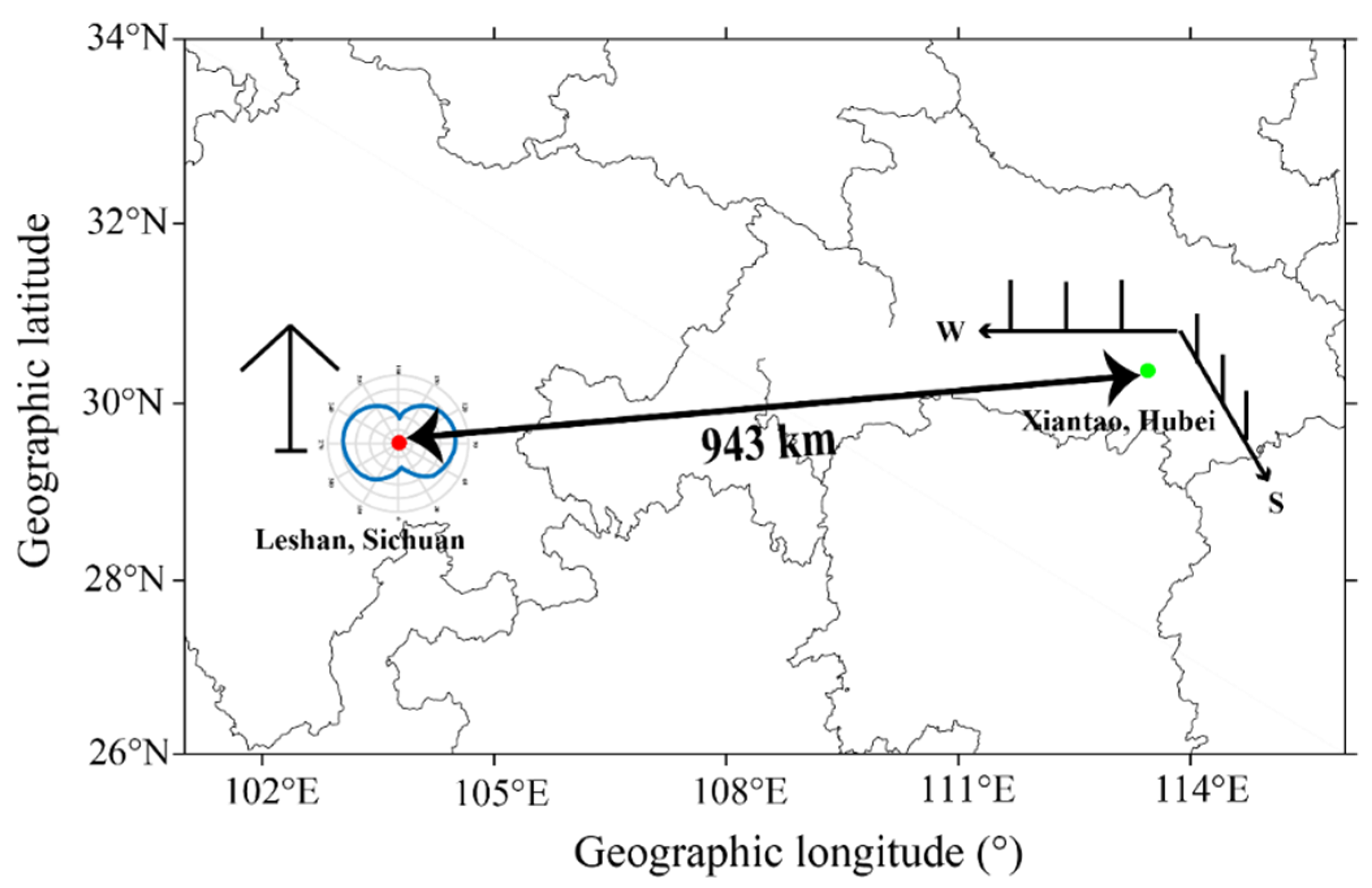
In order to verify the actual effect of the proposed scheme in this paper, the OIS signals used in this paper were transmitted from Leshan station and received by Xiantao multi-channel receiving system. The geographical location diagram of the transceiver station is shown in the Figure 9. The distance between the transceiver stations is about 943 km.

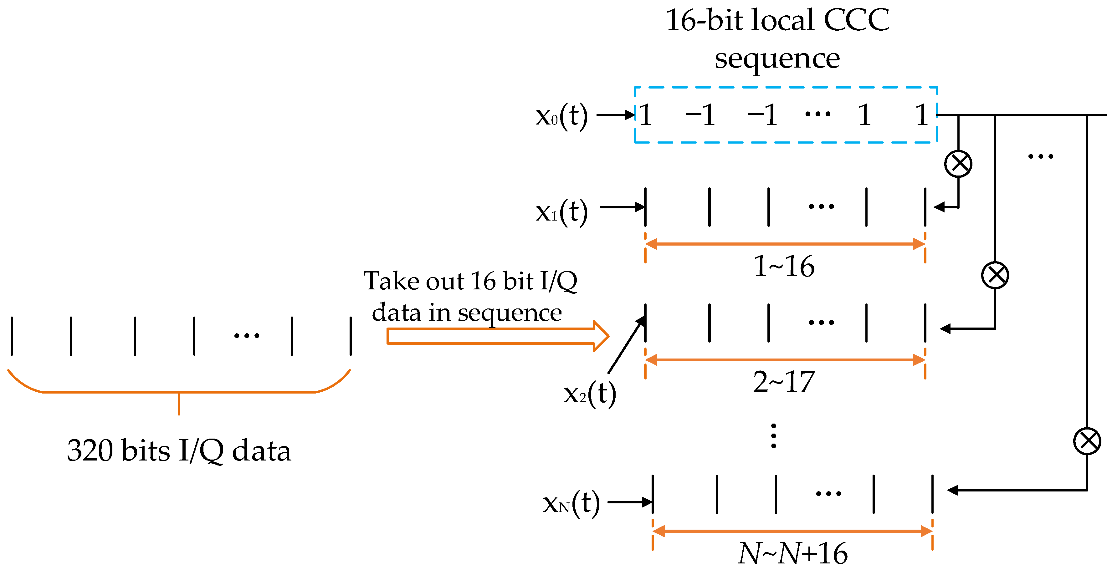
As CCC has excellent correlation characteristic and can obtain high compression gains, the transmitted signal is encoded with a 16-bit CCC sequence [29,30] in our experiments. The width t_p of each code chip is 25.6 us, so the original range resolution △R is 7.68 km, which is the size of each range bin.

The duty cycle of the transmitted signal is 5%, and it is modulated with 16-bit CCC, that is, there can be 320 range bins in one detection; namely the maximum value of N is 320.

In the experiment, the scanning step of the range spectrum is 0.768 km, while the resolution is improved by 10 times.

In the process of data segmentation of the cross spectrum X(f) and the reconstruction of the sample covariance matrix, we found that the strength of Capon spectrum is contradictory to the discrimination ability of signal through experiments. The higher the order of the covariance matrix and the smaller the number of snapshots of the segmented data, the weaker the strength of the Capon spectrum, but the stronger the discrimination ability of signal is, and vice versa. Therefore, to obtain a strong signal discrimination ability and to maintain a certain strength of the Capon spectrum, a compromise value for the order m of the covariance matrix needs to be specified. In this study, the order m is set to 128.

In order to verify the effect of the proposed scheme in this paper, we selected three sets of data at different fixed frequency points for testing and comparison: 7.6 MHz, 8.15 MHz, 11.05 MHz; in addition, we also tested a set of 6~15 MHz OIS data of swept frequency.

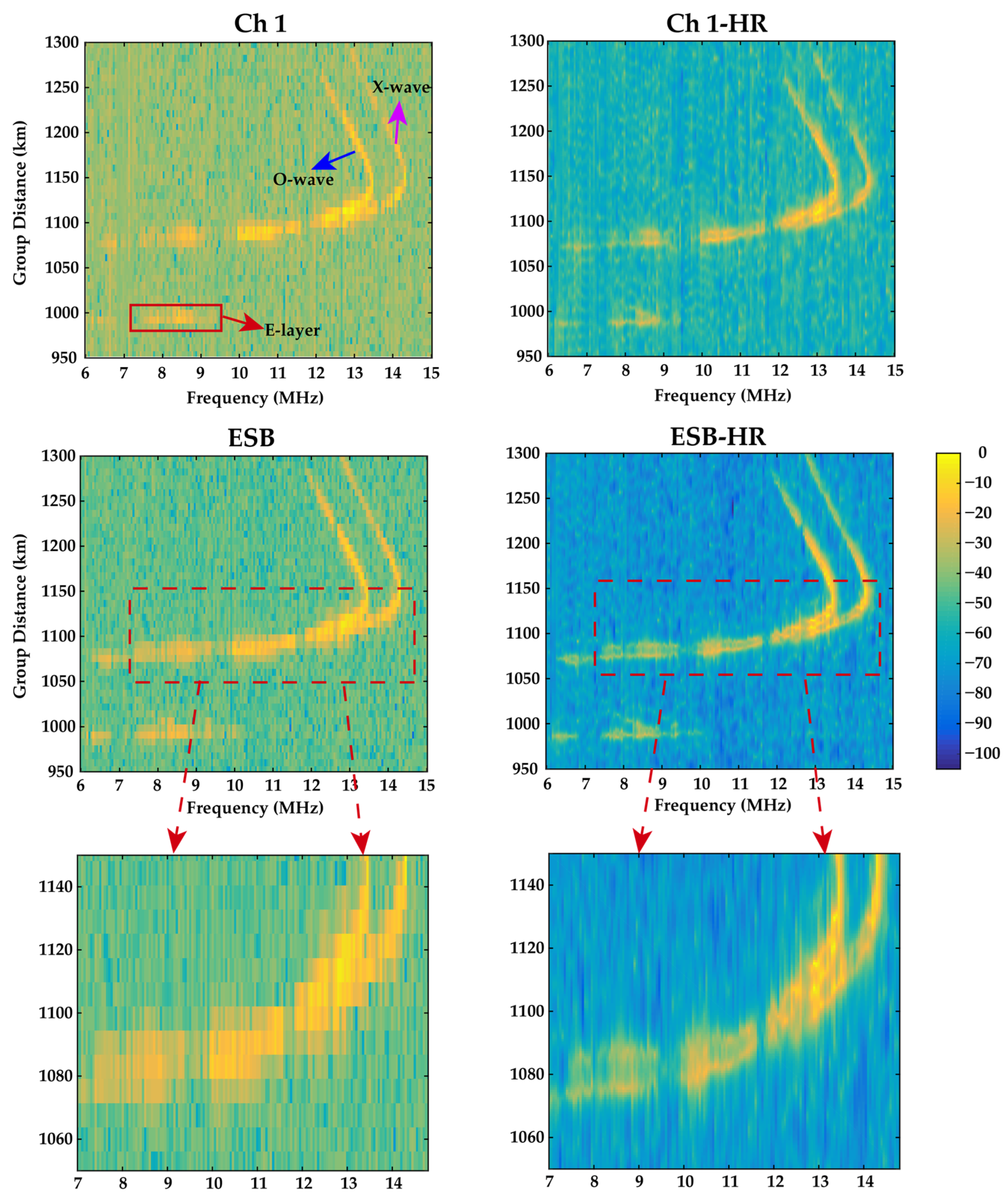
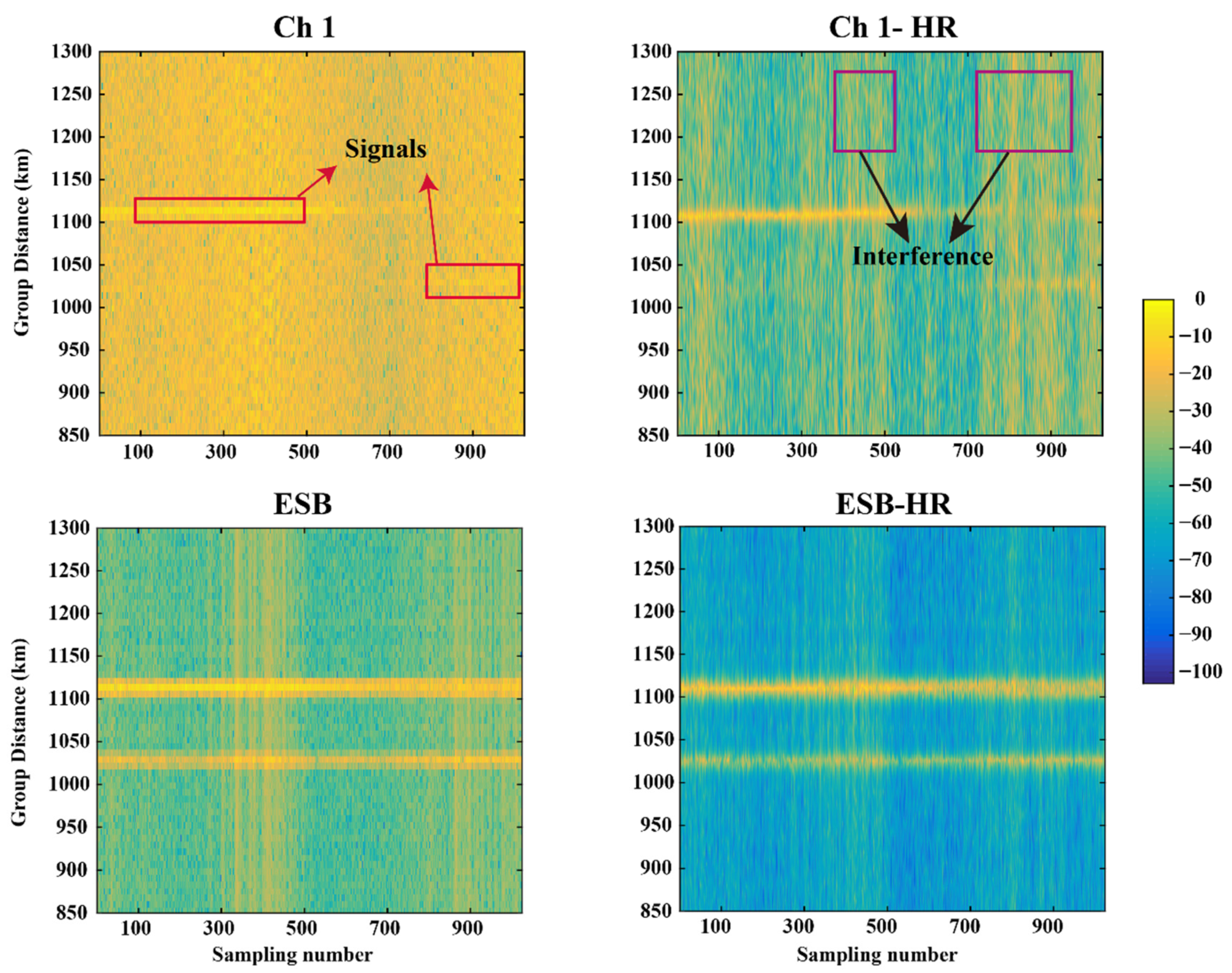
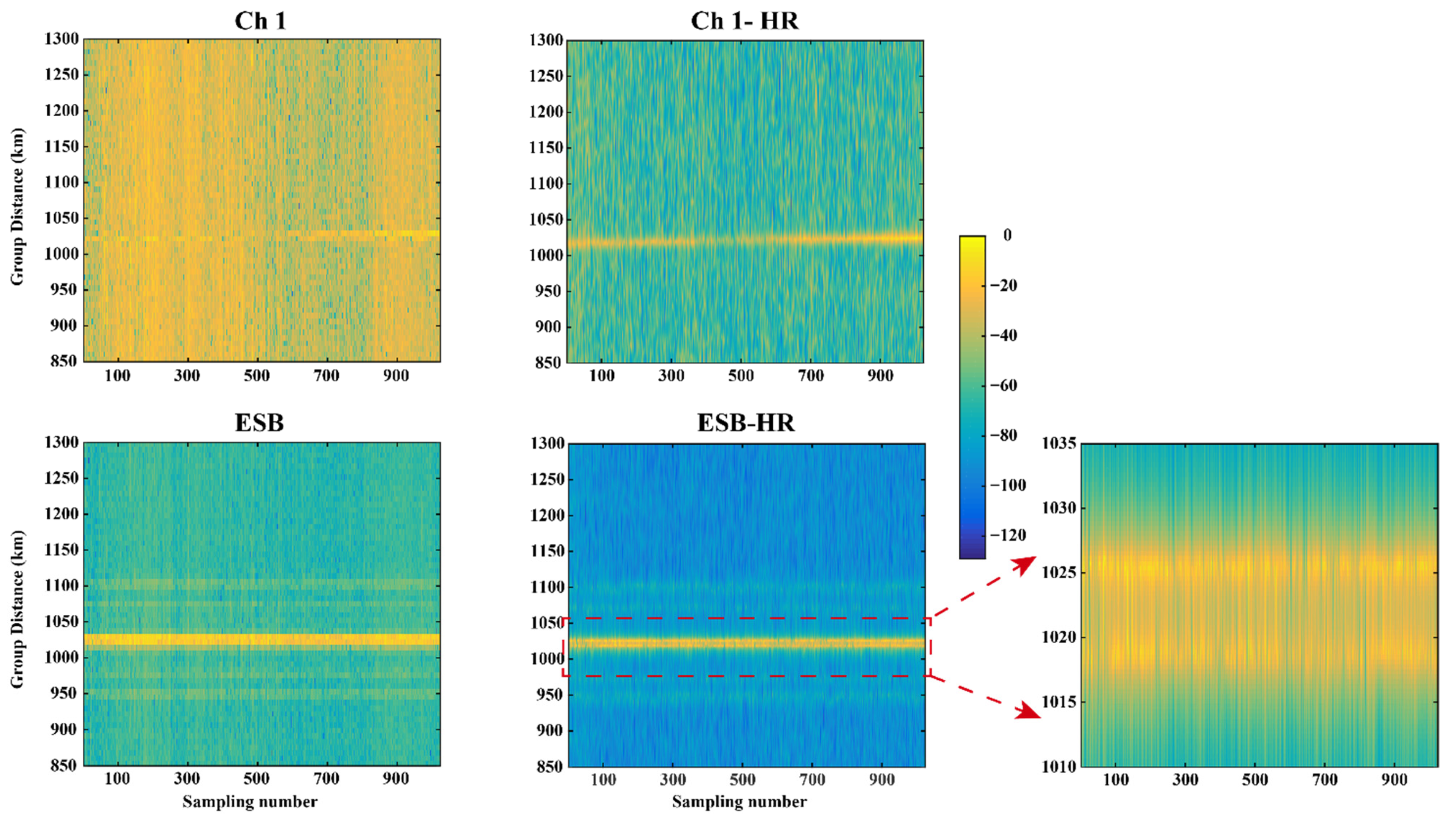
Figure 10 is the normalized ionogram of the 7.6 MHz OIS signal in different situations, this set of data was collected at 17:04:59 Beijing Time (BJT, UTC+8) on 13 January 2020; the sunrise time was 07:34:55 BJT and the sunset time was 17:10:35 BJT. Where “Ch 1” represents the OIS signal of Channel 1, “Ch 1-HR” represents that the range resolution of the OIS signal of Channel 1 is directly increased by 10 times through Capon HRRP algorithm, and “ESB” represents the signal of six channels after being processed by the ESB algorithm, ”ESB-HR” indicates that the signals of six channels are processed by Capon HRRP after ESB adaptive beamforming; the horizontal axis represents the number of sampling points of one detection, that is one range bin, and the vertical axis represents the group distance. It can be seen from the Figure 10 that the background noise and interference of Channel 1 are mixed together, and the mixed values are about −18 dB, which is relatively high, so that the desired signals are submerged and inconspicuous. Specifically, at a group distance of about 1029 km, the desired signal is almost invisible. When the signal of Channel 1 is processed by Capon HRRP, it can be seen that the background noise can be suppressed a lot. The average value is about −27 dB, which is 9 dB lower than the background noise of Channel 1. This is because the interference and noise have no correlation with the local code, so their phase spectrum does not have linear relationship as the Equation (12) between their frequency components of cross spectrum and the local code, resulting in great suppression in the Capon spectrum estimation. However, relatively speaking, the desired signal is more significantly enhanced, and the trace becomes much clearer after the six-channel signal is processed by the ESB adaptive beamforming algorithm, and the effect is better than the signal of Channel 1 only processed with Capon HRRP algorithm. Compared with Capon HRRP algorithm, the ESB algorithm has better suppression effect on interference and noise under the certain conditions. Moreover, when the synthesized signal by the ESB algorithm is processed by the Capon HRRP algorithm, it can be seen that the interference is almost suppressed, the background noise is significantly reduced, to only about −65 dB. In addition, some regions where the desired signal is very weak or even completely overwhelmed by interference and noise becomes much clearer. Furthermore, more details can be observed, such as the widening or compression of the group distance of the received signal and the fluctuation of echo energy. It will be very helpful for research on the fine structure and the spatial–temporal evolution process inside the ionosphere.

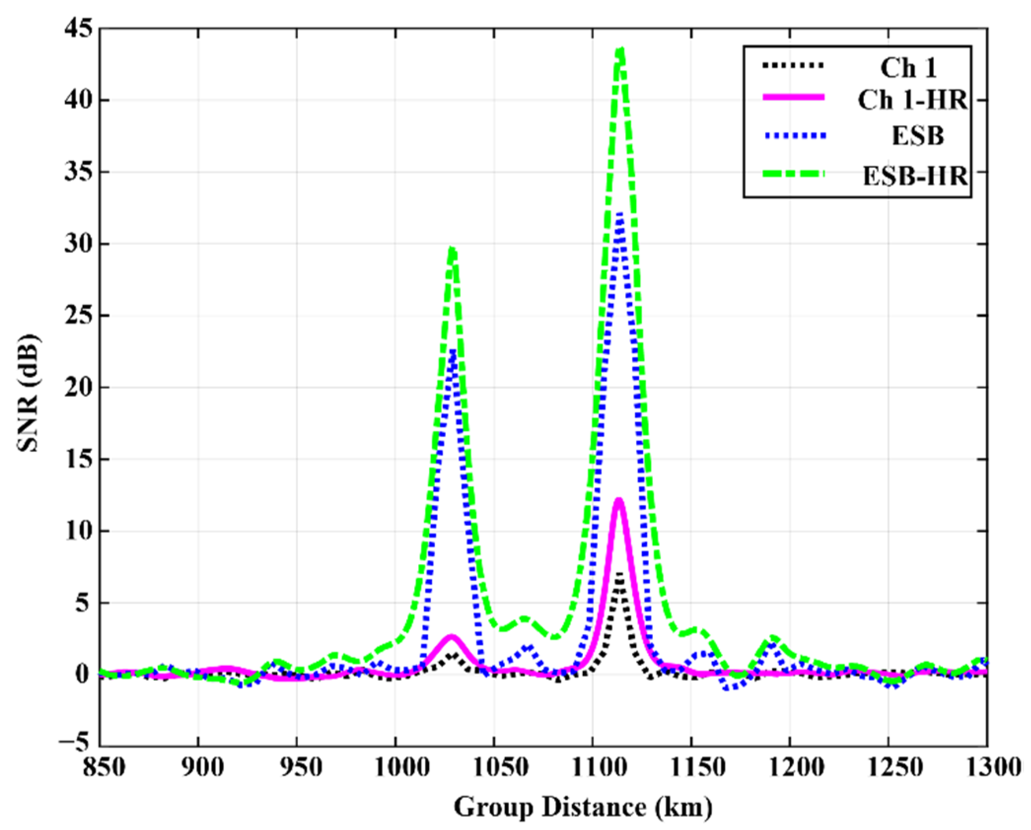
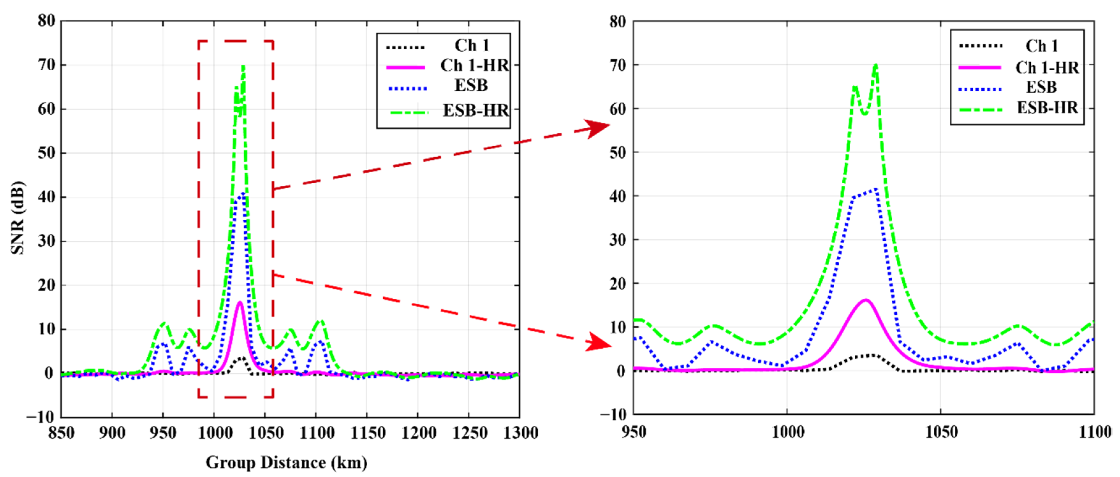
In order to reflect the improvement of SNR more intuitively, the background noise of each ionogram is set as a benchmark. Then, their SNRs can be compared more clearly, as shown in the following Figure 11.

It can be seen from Figure 11, compared with the echo signal of Ch 1, the SNR of ESB-HR at the group distance of 1029 km is improved by 28.28 dB, and by 36.62 dB at 1114 km. The improvement of SNR is obvious.

Moreover, a group of 11.05 MHz data is also tested this was collected at 13:08:59 BJT on 15 January 2020; the sunrise time was 07:34:16 BJT and the sunset time is 17:12:43 BJT. Figure 12 is the OIS ionogram of the 11.05 MHz echo signal, according to the formula of the earth’s great circle distance and curvature radius, it can be known that this echo comes from the Es-layer. It can be clearly seen that the SNR is increased, and the interference and noise are suppressed, so the trace of the echo signal is clearly visible. And the ionogram quality is greatly improved. Furthermore, it also should be noted that the echo signal was synthesized by ESB algorithm, and then the range resolution was increased by 10 times, not only is the SNR significantly improved, but also the details of the echo signal are more abundant and comprehensive. The stratification of the Es-layer can be clearly seen from the ionogram of ESB-HR, while the stratification cannot be observed from the ionogram of Ch 1. When a single imaging result is taken, as shown in Figure 13, it can be observed more clearly.

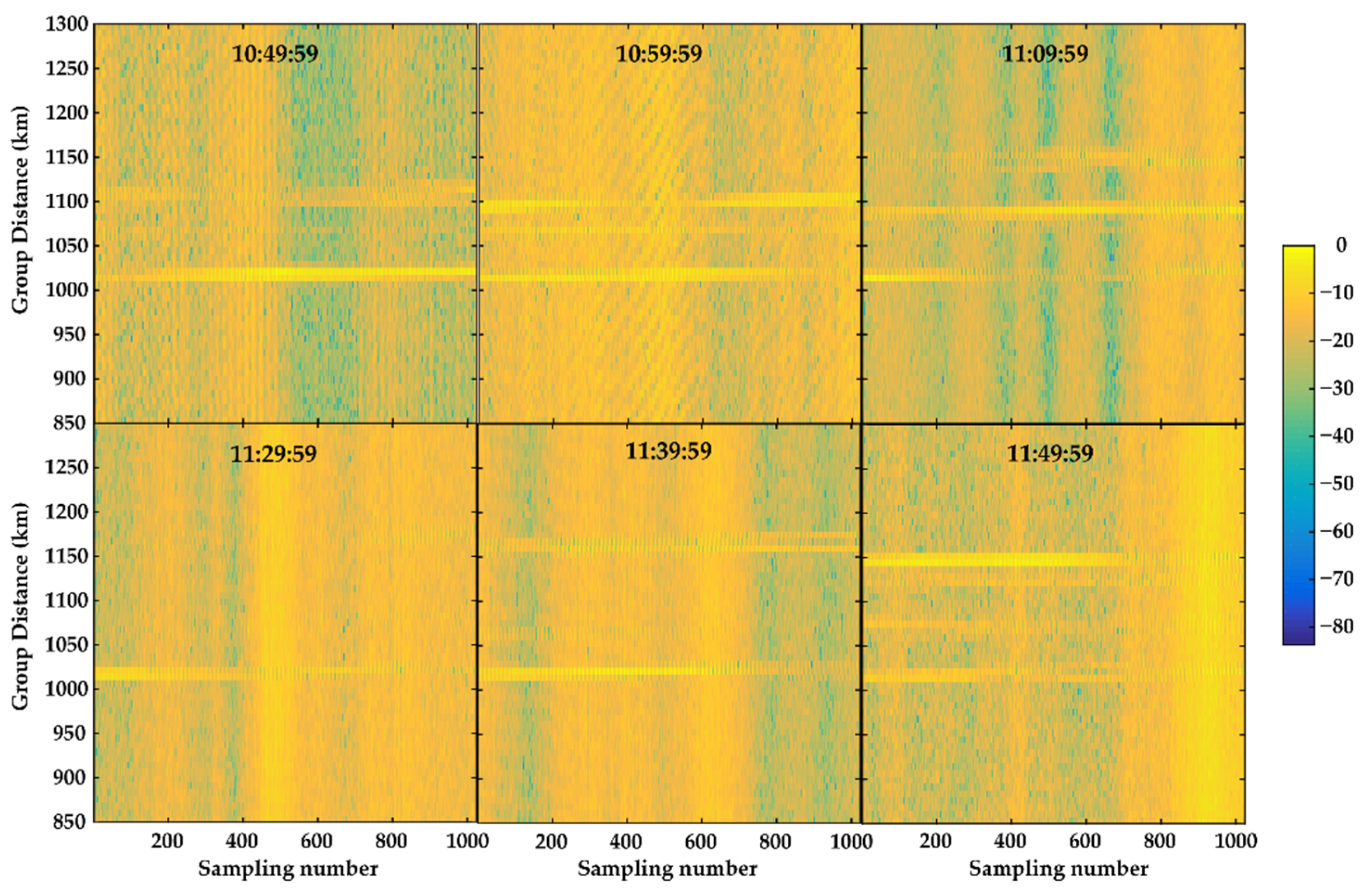
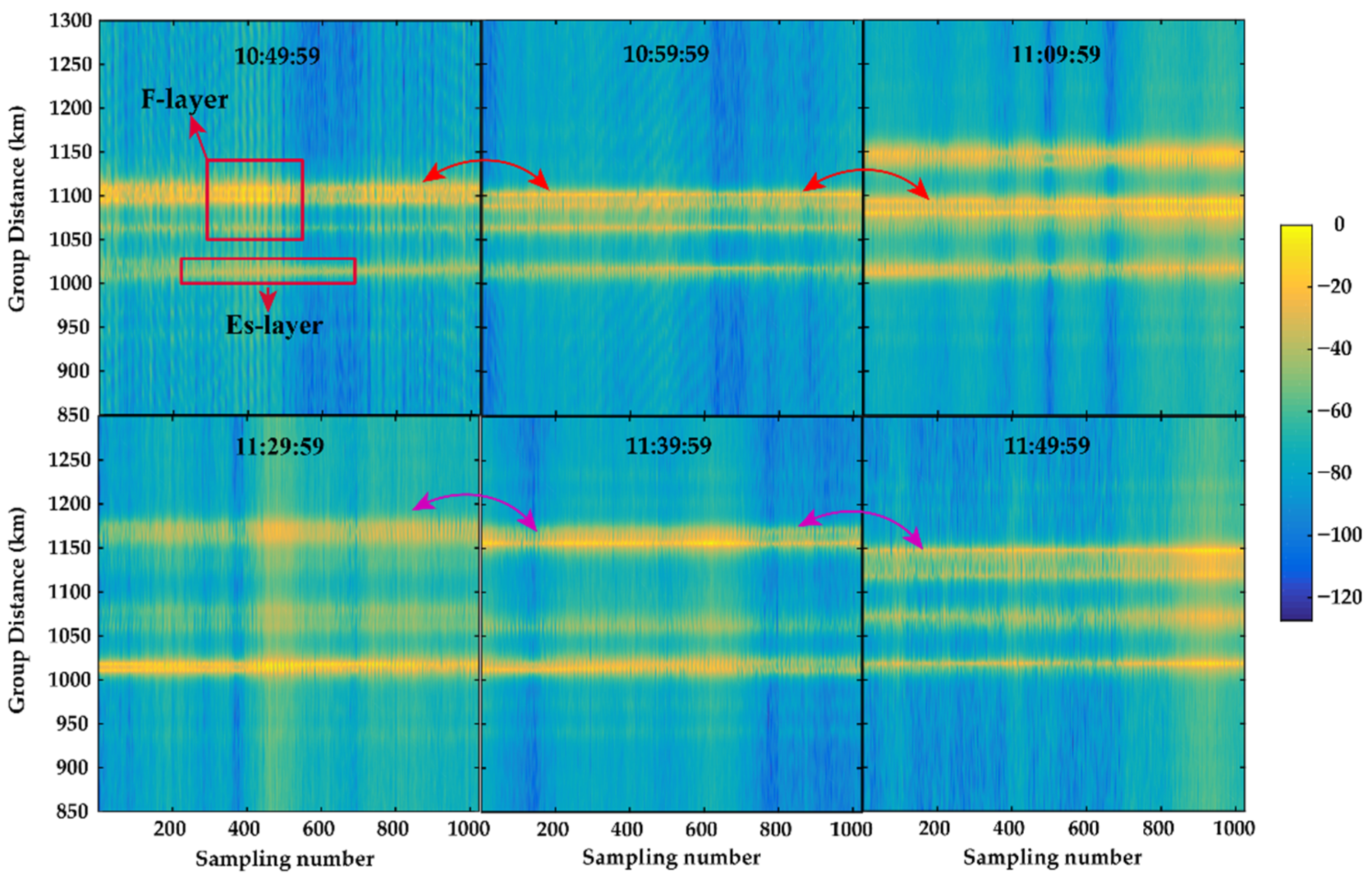
In addition, the movement of the ionosphere can also be monitored after improving the range resolution. As shown in Figure 14, the frequency is 8.15 MHz, from 10:49:59 to 11:49:59 BJT on 18 January 2020; the sunrise time is 07:33:01 BJT and the sunset time is 17:16:01 BJT. Figure 14 shows the OIS ionograms of a single channel at different times. As the ionogram quality and the range resolution is so poor, the traces can only be roughly identified, but the layered structures and finer movement process are difficult to describe. However, the ionogram quality can be significantly improved through the ESB and Capon HRRP algorithm. It can be noticed from Figure 15 that during the period of 10:49:59–11:09:59 BJT, even the movement speed of some layered or internal structure of the F-layer can be roughly estimated. Obviously, it benefits from the improvement of the range resolution and ionogram quality. It also means that the structure and movement inside the ionosphere can be observed more finely, and its evolution process can be monitored in real-time.

Figure 16 is the swept frequency OIS ionogram of 6~15 MHz, it comes from 12:24:59 BJT on 3 April 2021; the sunrise time is 05:55:08 BJT and the sunset time is 18:40:13 BJT. It can be seen from Figure 16 that the SNR of the echo signal has been improved to a certain extent only through Capon HRRP, and the echo trace also has some improvement. The echo trace is much clearer and more continuous after ESB algorithm processing. For example, the echo of the E-layer, which is almost invisible in Channel 1, become clearer after being processed by the ESB algorithm. However, the separation process of O-wave and X-wave in the F2-layer is not obvious at this condition. After the joint processing of ESB and Capon HRRP, it can be seen from the ionogram that the separation process of O-wave and X-wave is obvious in both the high-angle wave and low-angle wave part. The separation process is more obvious and the trace of the echo becomes narrower, which has the potential to reflect the change process of the ionosphere more accurately. At the same time, it is also very conducive to the accurate interpretation of the group distance, MUF, and other parameters.

7. Conclusions

Under the condition of compact antenna arrays, in methods of suppressing interference and noise to improve the quality of OIS ionogram, the Ionospheric Laboratory of Wuhan University has made preliminary achievements in this research direction [21,31]. However, following the improvement of the SNR of OIS ionogram, few researchers have paid attention to improve the range resolution of the OIS ionogram to observe the internal structure and spatiotemporal evolution inside the ionosphere with high precision. This paper has conducted research on this. The scheme proposed in this paper is based on using the ESB algorithm to improve the SNR of OIS ionogram, and then uses the Capon HRRP algorithm to improve the range resolution of OIS ionograms. The experimental results demonstrate that when the range resolution is significantly improved, the specific structure of the ionosphere and its spatial–temporal evolutions can be precisely observed with traditional OIS instruments. It is therefore of great significance to use this method to perform research into the internal structures and the occurrences of different scales and types of disturbances, as well as to explore the underlying physical mechanism.

Nevertheless, the coherent superposition of multi-mode oblique incident signals has not been considered during the processing of this method, which may have a certain deterioration on the imaging effect. The class of the smoothing algorithm for the covariance matrix may be a solution; however, methods to determine the smoothing order are still a problem worthy of consideration. It is also one of our future research objectives.

References

1. Alsina-Pagès, R.; Altadill, D.; Hervás, M.; Blanch, E.; Segarra, A.; Sans, X.G. Variation of Ionospheric Narrowband and Wideband Performance for a 12,760 km Transequatorial Link and Its Dependence on Solar and Ionospheric Activity. Remote Sens. 2020, 12, 2750. [Google Scholar] [CrossRef]
2. Chernogor, L.; Garmash, K.; Guo, Q.; Rozumenko, V.; Zheng, Y.; Luo, Y. Supertyphoon Hagibis action in the ionosphere on 6–13 October 2019: Results from multi-frequency multiple path sounding at oblique incidence. Adv. Space Res. 2021, 67, 2439–2469. [Google Scholar] [CrossRef]
3. Frazer, G.J. Experimental results for MIMO methods applied in over-the-horizon radar. IEEE Aerosp. Electron. Syst. Mag. 2017, 32, 52–69. [Google Scholar] [CrossRef]
4. Chernogor, L.F.; Garmash, K.P.; Guo, Q.; Rozumenko, V.T.; Zheng, Y. Passive Radar for Oblique-Incidence Ionospheric Sounding: Observations of Ionospheric Storms. In Proceedings of the IEEE Ukrainian Microwave Week (UkrMW), Kharkiv, Ukraine, 21–25 September 2020; pp. 253–258. [Google Scholar] [CrossRef]
5. Maeda, J.; Heki, K. Two-dimensional observations of midlatitude sporadic E irregularities with a dense GPS array in Japan. Radio Sci. 2013, 49, 28–35. [Google Scholar] [CrossRef]
6. Hysell, D.; Nossa, E.; Aveiro, H.; Larsen, M.; Munro, J.; Sulzer, M.; González, S. Fine structure in midlatitude sporadic E layers. J. Atmos. Sol.-Terr. Phys. 2013, 103, 16–23. [Google Scholar] [CrossRef]
7. Athparia, R.; Devi, M.; Barbara, A.K. Role of EQ preparatory processes on ionospheric parameters through analysis of ionization density of Spread F-layer and Sporadic E. Indian J. Phys. 2021, 96, 357–371. [Google Scholar] [CrossRef]
8. Takahashi, H.; Espaciais, S.J.d.C.I.N.d.P.; Essien, P.; Figueiredo, C.A.O.B.; Wrasse, C.M.; Barros, D.; Abdu, M.A.; Otsuka, Y.; Shiokawa, K.; Li, G. Multi-instrument study of longitudinal wave structures for plasma bubble seeding in the equatorial ionosphere. Earth Planet. Phys. 2021, 5, 368–377. [Google Scholar] [CrossRef]
9. Restano, M.; Mastrogiuseppe, M.; Masdea, A.; Picardi, G.; Seu, R. Ionosphere compensation and stepped frequency processing in the MARSIS experiment. In Proceedings of the Microwaves, Radar & Remote Sensing Symposium, Kiev, Ukraine, 25–27 August 2011; pp. 149–152. [Google Scholar] [CrossRef]
10. Tian, Y.; Hu, C.; Dong, X.; Zeng, T.; Long, T.; Lin, K.; Zhang, X. Theoretical Analysis and Verification of Time Variation of Background Ionosphere on Geosynchronous SAR Imaging. IEEE Geosci. Remote Sens. Lett. 2014, 12, 721–725. [Google Scholar] [CrossRef]
11. Du, L.; Chen, J.; Hu, J.; Li, Y.; He, H. Statistical Modeling with Label Constraint for Radar Target Recognition. IEEE Trans. Aerosp. Electron. Syst. 2019, 56, 1026–1044. [Google Scholar] [CrossRef]
12. Jangal, F.; Saillant, S.; Helier, M. Ionospheric clutter cancellation and wavelet analysis. In Proceedings of the 2006 First European Conference on Antennas and Propagation, Nice, France, 6–10 November 2006; pp. 1–6. [Google Scholar] [CrossRef]
13. Liu, A.-J.; Mao, X.-P.; Deng, W.-B. Oblique projection polarization filtering and its performance in High Frequency Surface Wave Radar. In Proceedings of the International Conference on Microwave & Millimeter Wave Technology, Chengdu, China, 8–11 May 2010; pp. 1618–1621. [Google Scholar] [CrossRef]
14. Xiang, Z.; Chen, B.; Yang, M. Transmitter/receiver polarisation optimisation based on oblique projection filtering for mainlobe interference suppression in polarimetric multiple-input–multiple-output radar. IET Radar Sonar Navig. 2018, 12, 137–144. [Google Scholar] [CrossRef]
15. Turley, M.D.E.; Heitmann, A.J.; Gardiner-Garden, R.S. Ionogram RFI Rejection Using an Autoregressive Interpolation Process. Radio Sci. 2019, 54, 135–150. [Google Scholar] [CrossRef]
16. Slomka, S.; Gibbins, D.; Gray, D.; Haywood, B. Features for high resolution radar range profile based ship classification. In Proceedings of the International Symposium on Signal Processing & Its Applications, Brisbane, QLD, Australia, 22–25 August 1999. [Google Scholar] [CrossRef]
17. Zhang, X.-D.; Shi, Y.; Bao, Z. A new feature vector using selected bispectra for signal classification with application in radar target recognition. IEEE Trans. Signal Process. 2001, 49, 1875–1885. [Google Scholar] [CrossRef]
18. Kim, K.-T.; Seo, D.-K.; Kim, H.-T. Efficient radar target recognition using the MUSIC algorithm and invariant features. IEEE Trans. Antennas Propag. 2002, 50, 325–337. [Google Scholar] [CrossRef]
19. Pilcher, C.M.; Khotanzad, A. Maritime ATR using Classifier Combination and High Resolution Range Profiles. IEEE Trans. Aerosp. Electron. Syst. 2011, 47, 2558–2573. [Google Scholar] [CrossRef]
20. Wang, J.; Liu, Z.; Xie, R.; Ran, L. Radar HRRP Target Recognition Based on Dynamic Learning with Limited Training Data. Remote Sens. 2021, 13, 750. [Google Scholar] [CrossRef]
21. Zhang, W.; Liu, T.; Yang, G.; Jiang, C.; Hu, Y.; Zhu, X.; Lan, T.; Zhao, Z. The Application of Beamforming Technology in Ionospheric Oblique Incidence Sounding with Wuhan Multi-Channel Ionospheric Sounding System (WMISS). IEEE Geosci. Remote Sens. Lett. 2021, 19, 8016205. [Google Scholar] [CrossRef]
22. Liu, T.; Yang, G.; Zhao, Z.; Jiang, C.; Hu, Y. Application of Beamforming Technology in Ionospheric Oblique Backscatter Sounding with a Miniaturized L-Array. Remote Sens. 2020, 12, 499. [Google Scholar] [CrossRef]
23. Weber, R.J.; Huang, Y. Analysis for Capon and MUSIC DOA estimation algorithms. In Proceedings of the IEEE Antennas and Propagation Society International Symposium, North Charleston, SC, USA, 1–5 June 2009; pp. 1–4. [Google Scholar] [CrossRef]
24. Lin, J.-D.; Fang, W.-H.; Wang, Y.-Y.; Chen, J.-T. FSF MUSIC for Joint DOA and Frequency Estimation and Its Performance Analysis. IEEE Trans. Signal Process. 2006, 54, 4529–4542. [Google Scholar] [CrossRef]
25. Fabrizio, G.A.; Gershman, A.; Turley, M. Robust adaptive beamforming for HF surface wave over-the-horizon radar. IEEE Trans. Aerosp. Electron. Syst. 2004, 40, 510–525. [Google Scholar] [CrossRef]
26. Bai, C.; Xu, S.; Duan, J.; Jing, B.; Yang, M.; Wan, M. Pulse-Inversion Subharmonic Ultrafast Active Cavitation Imaging in Tissue Using Fast Eigenspace-Based Adaptive Beamforming and Cavitation Deconvolution. IEEE Trans. Ultrason. Ferroelectr. Freq. Control 2017, 64, 1175–1193. [Google Scholar] [CrossRef]
27. Yang, G.; Liu, T.; Zhou, A.; Jiang, C.; Hu, Y.; Zhao, Z.; Ni, B. A Novel Land-Based High-Frequency Geolocation System. IEEE Geosci. Remote Sens. Lett. 2020, 18, 48–52. [Google Scholar] [CrossRef]
28. ShahbazPanahi, S.; Gershman, A.; Giannakis, G. Semiblind multiuser MIMO channel estimation using capon and MUSIC techniques. IEEE Trans. Signal Process. 2006, 54, 3581–3591. [Google Scholar] [CrossRef]
29. Yang, G.; Duan, P.; Jiang, C.; Liu, T.; Lan, T.; Zhao, Z.; Shi, S.; Xu, C. Application of Biphase Complete Complementary Code for Ionospheric Sounding. Sensors 2018, 18, 2811. [Google Scholar] [CrossRef] [PubMed]
30. Liu, T.; Yang, G.; Hu, Y.; Jiang, C.; Lan, T.; Zhao, Z.; Ni, B. A Novel Ionospheric Sounding Network Based on Complete Complementary Code and Its Application. Sensors 2019, 19, 779. [Google Scholar] [CrossRef] [Green Version]
31. Shi, S.-Z.; Chen, G.; Yang, G.-B.; Li, T.; Zhao, Z.-Y.; Liu, J.-N. Wuhan Ionospheric Oblique-Incidence Sounding System and Its New Application in Localization of Ionospheric Irregularities. IEEE Trans. Geosci. Remote Sens. 2015, 53, 2185–2194. [Google Scholar] [CrossRef]
Figure 1. Structural diagram of WMISS.
Remotesensing 14 04305 g001
Figure 2. The compacted “L-shape” array: (a) the received array outdoor; (b) schematic diagram of antenna direction and spacing.
Remotesensing 14 04305 g002
Figure 3. The signal processing part of the indoor equipment.
Remotesensing 14 04305 g003
Figure 4. The control part of the upper computer.
Remotesensing 14 04305 g004
Figure 5. Data processing scheme and flow.
Remotesensing 14 04305 g005
Figure 6. A general beamformer.
Remotesensing 14 04305 g006
Figure 7. Range difference model based on received signal.
Remotesensing 14 04305 g007
Figure 8. Schematic diagram of bandwidth division of echo signal.
Remotesensing 14 04305 g008
Figure 9. The geographical location diagram of the transceiver station.
Remotesensing 14 04305 g009
Figure 10. The OIS ionogram of 7.6 MHz under different conditions.
Remotesensing 14 04305 g010
Figure 11. Comparison of SNR at 7.6 MHz under different conditions after subtracting background noise.
Remotesensing 14 04305 g011
Figure 12. The OIS ionogram of 11.05 MHz under different conditions.
Remotesensing 14 04305 g012
Figure 13. Comparison of SNR at 11.05 MHz under different conditions after subtracting background noise.
Remotesensing 14 04305 g013
Figure 14. The OIS ionogram of a single channel from 10:49:59 to 11:49:59.
Remotesensing 14 04305 g014
Figure 15. The OIS ionogram of ESB-HR from 10:49:59 to 11:49:59.
Remotesensing 14 04305 g015
Figure 16. Comparison of OIS signal of 6~15 MHz swept frequency processed by different algorithms.
Remotesensing 14 04305 g016