Contributions of Climate Change, Vegetation Growth, and Elevated Atmospheric CO₂ Concentration to Variation in Water Use Efficiency in Subtropical China

Abstract

Ecosystem water use efficiency (WUE) plays an important role in maintaining the carbon assimilation–water transpiration balance in ecosystems. However, spatiotemporal changes in WUE in the subtropical region of China (STC) and the impact of driving forces remain unclear. In this study, we analyzed the spatiotemporal variation in WUE in the STC and used ridge regression combined with path analysis to identify direct and indirect effects of climate change, vegetation growth, and elevated atmospheric CO₂ concentration (Ca) on the interannual trend in WUE. We then quantified the actual and relative contributions of these drivers to WUE change based on the sensitivity of these variables on WUE and the trends of the variables themselves. Results reveal a mean WUE of 1.57 g C/m²/mm in the STC. The annual WUE series showed a descending trend with a decline rate of 0.0006 g C/m²/mm/year. The annual average temperature (MAT) and leaf area index (LAI) had strong positive direct effects on the WUE, while the vapor pressure deficit (VPD) had a strong negative direct effect. Opposite direct and indirect effects offset each other, but overall there was a total positive effect of Ca and VPD on WUE. In terms of actual contribution, LAI, Ca, and VPD were the main driving factors; LAI caused WUE to increase by 0.0026 g C/m²/mm/year, while Ca and VPD caused WUE to decrease by 0.0021 and 0.0012 g C/m²/mm/year, respectively. In terms of relative contribution, LAI dominated the WUE trend, although Ca and VPD were also important factors. Other drivers contributed less to the WUE trend. The results of this study have implications for ecological management and restoration under environmental climate change conditions in subtropical regions worldwide.

1. Introduction

The conflict between the gain in carbon (through photosynthesis) and loss of water (through transpiration) in plants or terrestrial ecosystems is referred to as water use efficiency (WUE), which is an important component of ecosystem function [1,2,3]. By quantifying spatiotemporal changes in WUE and identifying its drivers, ecosystem responses to changing environments can be revealed, which has important implications for management of ecosystems [4,5].

WUE is defined as the ratio of Gross Primary Productivity (GPP) and evapotranspiration (ET), and there are several ways to estimate GPP and ET. For example, the eddy covariance technique is used for field measurements, evaluation based on a data mining model or process model, and estimation through remote sensing products [6]. Given that observed data are very sparse and limit the data mining model’s function, remote sensing data are currently one of the most commonly used methods for estimating GPP and ET at the regional scale [7]. Many studies have confirmed the applicability of remote sensing data in GPP and ET estimation [5,8,9,10,11].

Changes in WUE are the combined result of changes in GPP and ET and the drivers that affect them. The photosynthetic utilization rate of vegetation can be improved by increasing the photosynthetic rate of vegetation. When the CO₂ absorption rate of leaf stomata reaches saturation, transpiration may be reduced by the reduction in leaf stomata [12]. Sunlight, rainfall, and temperature are important climatic factors that affect the photosynthetic rate of vegetation [8,13]; CO₂ is an important participant in vegetation photosynthesis, and elevated atmospheric CO₂ concentration (Ca) will have a fertilizing effect on plant growth [4]. An increase in vapor pressure deficit may cause reductions in stomatal conductance and photosynthetic rates in vegetation [14,15]. The leaf area index (LAI) can be used as an important indicator of vegetation growth. Increasing LAI leads to increasing ET by affecting canopy transpiration and interception, decreasing the proportion of solar radiation reaching the surface of the soil and decreasing evaporation of bare soil, thereby reducing ET [16]. In addition, plants extract water from the soil, and vegetation growth can be affected by the availability of soil moisture [17,18]. The mechanisms regulating changes in WUE are driven by the highly complex interplay between climatic environmental changes and vegetation growth. In theory, environmental variables impacting GPP or ET can also impact WUE. Potential controlling factors for WUE include air temperature, precipitation, LAI, shortwave radiation, vapor pressure deficit, soil content of water, and atmospheric CO₂ content [7,19,20,21,22].

Scholars have investigated the driving factors underlying WUE. Sun et al. (2016) explored the spatial relationship between global WUE and climate variables through regression analysis [23]. Yang et al. (2021) further analyzed the global annual WUE response to the drought index using Spearman correlation analysis [24]. Subrata et al. (2022) used a random forest algorithm to analyze the control of various biometeorological drivers in WUE for various forest type groups in India [25]. Sun et al. (2021) and Zhao et al. (2022) identified the driving factors of various WUE changes in China through a sensitivity analysis, and argued that vegetation growth and elevated atmospheric CO₂ emissions are the main factors underlying WUE changes in China [26,27,28]. Most studies employing partial correlation analysis or simple correlation have found that the spatial distributions of climate variables show strong correlations with those of WUE [26]. However, the actual contribution of each driver to WUE dynamics remains unknown. The variation trend of WUE cannot be determined solely by the correlation strength between the driving factor and WUE; rather, the trends in drivers, including trends in quantity and direction, must be considered. Each driver’s contribution to the trend in WUE change includes not only the influence of the relationship but also the direction and degree of the change trend of the driver. Based on the sensitivity of WUE to these variables, using the changing trends of the variables themselves to assess contributions can prevent underestimating the contributions of weakly sensitive factors. The dominant factors that influence WUE dynamics can be identified by comparing the contribution of each driver to WUE dynamics. At the same time, the multiple driving factors are interlinked and often jointly regulate the WUE of an ecosystem; therefore, analyzing the control mechanisms of WUE is often difficult. The multiple regression method is commonly utilized to enumerate the contributions of environmental drivers. Although multiple regression is often impacted by the challenge of multicollinearity, ridge regression can effectively eliminate factor collinearity [7,8]. Moreover, apart from its direct effects, environmental variables may also exert indirect effects on WUE through mediating variables. For example, vapor pressure deficit (VPD) directly impacts the characteristics of plant physiology (such as stomatal conductance) as a transient change in GPP and ET, but can also show a delayed impact on WUE by modulating plant phenology and canopy structure; in this process, LAI is the mediating variable [19]. Path analysis has proven to be very effective in assessing both the indirect and direct impacts of assumed causality [1,28].

Approximately 25% of China’s land area contains subtropical forests typified by elevated biodiversity, special types of vegetation, and unique ecological functions; this forest area plays a key function in maintaining the region’s ecological balance [29]. Understanding the water–carbon coupling relationship of vegetation and its driving mechanisms is crucial. However, previous studies have mainly focused on the temporal and spatial variation characteristics of WUE and its relationship with precipitation and temperature [30]. The response of WUE to climate change, vegetation growth, and elevated atmospheric CO₂ concentration remains unclear, especially in the subtropical region of China (STC). Therefore, the goals of this study were as follows: (1) to assess interannual variations in the WUE of the subtropical region of China from 1982 to 2018; (2) to analyze the direct and indirect effects of climate change, vegetation growth, and elevated atmospheric CO₂ concentration on WUE trends; and (3) to estimate relative and actual contributions of drivers to WUE change. It was hypothesized that the interannual variation in WUE was mostly controlled by vegetation growth (as represented by LAI). By studying changes in WUE within different landscape types and the underlying mechanisms, the interaction between ecosystems and climate change will be better understood. As such, the results of this study offer a scientific reference for ecological management and restoration of the STC under climate change.

2. Materials and Methods

2.1. Data and Preprocessing

The present study used GPP, ET, and LAI data with a 0.05° spatial resolution for 1982–2018 obtained from Global Land Surface Satellite (GLASS) products [31,32]. To ensure the reliability of the data, FLUXNET tower data were used to verify the GPP and ET values in the STC (Figure S1). Meteorological data were obtained from the National Tibetan Plateau Data Center (2019). This dataset, with a temporal and spatial resolution of 3 h and 0.1°, respectively, was compiled through a combination of remote sensing data, field station data, and data reanalysis. Included in the dataset are data for seven near-surface climate variables, namely surface pressure, air temperature, specific humidity, downward shortwave radiation, wind speed, downward long-wave radiation, and rate of precipitation [33,34]. In this study, we used average annual temperature (MAT), annual accumulated precipitation (MAP), and annual solar radiation (Rg) data to analyze the impact of climate change on WUE dynamics. VPD data were derived from the Google Earth Engine (GEE) Terra Climate, which provides a climate water balance for terrestrial surfaces at a global scale and monthly resolution [25]. Soil water content (SWC) was obtained from the GLDAS Noah Land Surface Model L4 monthly 0.25 × 0.25° V2.0. Atmospheric CO₂ concentration data were sourced from the Center for Global Environmental Research. Climate zone and landscape data were sourced from the Resource Environmental Science and Data Center. Climate zoning data were used to determine the extent of the STC. For convenience of research, the landscape was divided into evergreen coniferous forest (ECF), evergreen broadleaf forest (EBF), deciduous broadleaf forest (DBF), shrub, grassland, and cropland (Figure S1). All datasets were resampled to 0.05 × 0.05°. To facilitate comparisons between the variables of different units and magnitudes, we normalized all variables based on the time series.

2.2. Methods

2.2.1. WUE

The WUE (g C/m²/mm) of an ecosystem can be defined as the GPP (g C/m²/year)-to-ET (mm/year) ratio [26,35]:

$$WUE=\frac{GPP}{ET}$$

(1)

2.2.2. Trend Analysis

Determination of annual trends in WUE and drivers over the period 1982−2018 was based on a least-square linear regression model. The trend function is:

$$Slope=\frac{n{{\displaystyle \sum }}_{i=1}^n\left(i\times X_i\right)-{{\displaystyle \sum }}_{i=1}^{n}i\times {{\displaystyle \sum }}_{i=1}^n{X}_i}{n\times {{\displaystyle \sum }}_{i=1}^n{i}^2-{({{\displaystyle \sum }}_{i=1}^{n}i)}^2}$$

(2)

In Equation (2), $i$ represents a single year, and varies between 1 and 37; $X_i$ represents WUE and drivers in year i; and n is the total number of years (37). For slope values > 0, $X$ increases; and for slope values < 0, $X$ decreases. An F-test was used to detect the significance of the trends, and p-values < 0.05 were considered significant [36,37].

2.2.3. Ridge Regression

Collinearity among the independent variables during multiple linear regression can result in least-squares estimation errors [38]. The present study overcame this challenge by using ridge regression, which effectively considers collinearity to identify more reliable coefficients compared to those by estimates of least-squares through the introduction of a ridge parameter [7]. The present study used five-fold cross validation to select the ridge parameter. The explanatory variables included the annual-scale potential drivers of WUE, including the MAT, MAP, Rg, SWC, VPD, Ca, and LAI. The dependent variable was the annual WUE.

2.2.4. Path Analysis

Path analysis can be categorized as a multivariate statistical method that can be applied to investigate relationships among multiple variables. Path analysis can be used to quantify the direct and indirect impacts of driving variables on dependent variables [7,28]. The present study applied path analysis to identify the relative indirect and direct impacts of climate change, vegetation growth, and elevated Ca on ecosystem-scale WUE.

A system demonstrating a relationship containing a single response variable, $y$, and driving variables $x_i$ ($i=1,2,\dots ,n)$ can be represented as:

$$\mathrm{y}={\alpha }_0+{\alpha }_1{x}_1+{\alpha }_2{x}_2+\cdots +{\alpha }_n{x}_n$$

(3)

The equation for the regular matrix according to Equation (3) can be written as:

$$\left[\begin{array}{cccc}1& r_{x_1{x}_2}& \cdots & r_{x_1{x}_n}\\ r_{x_2{x}_1}& 1& \cdots & r_{x_2{x}_n}\\ ⋮& ⋮& \ddots & ⋮\\ r_{x_n{x}_1}& r_{x_n{x}_2}& \cdots & 1\end{array}\right]·\left[\begin{array}{c}{\alpha }_1\\ {\alpha }_2\\ ⋮\\ {\alpha }_n\end{array}\right]=\left[\begin{array}{c}{\beta }_1\\ {\beta }_2\\ ⋮\\ {\beta }_n\end{array}\right]$$

(4)

where $r_{x_i{x}_j}$ represents the simple coefficient of correlation of $x_i$ and $x_j$, ${\alpha }_i$ is the direct path coefficient of $x_i$ to $y$, and $r_{x_i{x}_j}·{\alpha }_i$ is the coefficient of the indirect path, reflecting the indirect impact of variable $x_i$ through variable $x_j$ to $y$ [39].

2.2.5. Contribution Analysis

The partial first-order derivative of each regression predictor can be termed a “sensitivity parameter”. Therefore, the sensitivity parameter equated to the ridge regression coefficient, and this parameter indicated changes to the response variable resulting from variations in the corresponding driver [38]. Simultaneously, the linear trend evident in the driving variable is representative of the average variation per unit of time. Therefore, changes to the dependent variable due to the unit time driving variable are enumerated as the product of the linear trend and sensitivity parameter, referred to as contribution of the driver to the dependent variable [7].

The impacts of drivers on WUE were enumerated using the ridge regression coefficient and the trends in the drivers:

$${\eta }_{c1}={\alpha }_1\ast X_{1s\_trend}$$

(5)

where ${\eta }_{c1}$ is the contribution of the normalized WUE variation, ${\alpha }_1$ is the ridge regression coefficient, and $X_{1s trend}$ is the trend evident in the independent normalized factor.

The present study confirmed the actual and relative contributions of different drivers to WUE:

$${\eta }_{rc1}=\frac{{\eta }_{c1}}{\left|{\eta }_{c1}\right|+\left|{\eta }_{c1}\right|+\left|{\eta }_{c1}\right|+\cdots }$$

(6)

$${\eta }_{ac1}=\frac{{\eta }_{c1}}{WU{E}_{s\_trend}}\ast WU{E}_{trend}=\frac{{\alpha }_1\ast X_{1s\_trend}}{WU{E}_{s\_trend}}\ast WU{E}_{trend}$$

(7)

where ${\eta }_{rc1}$ represents the proportional contribution of $X_1$ to the WUE trend, ${\eta }_{ac1}$ represents the contribution to variation in WUE, $WU{E}_{s\_trend}$ is the normalized WUE trend, and $WU{E}_{trend}$ is the trend of WUE [8].

To facilitate the comparative analysis, during the identification of dominant factors, this study considered the combined effects of the MAT, MAP, Rg, SWC, and VPD as the climate change (Cli) effects and that of LAI variations and elevated Ca as separate factors to characterize vegetation growth and environmental change, including Cli, LAI variations, and elevated Ca. In addition, if a factor (e.g., Cli, LAI, or Ca) had a relative contribution rate of more than 50% to the change in WUE in the corresponding pixel, this factor could be used as the dominant factor; moreover, if the sum of the relative contribution rates of the two factors exceeded 80%, then the combination of these factors was considered a dominant factor. The others were balanced by three factors.

3. Results

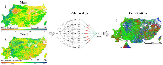
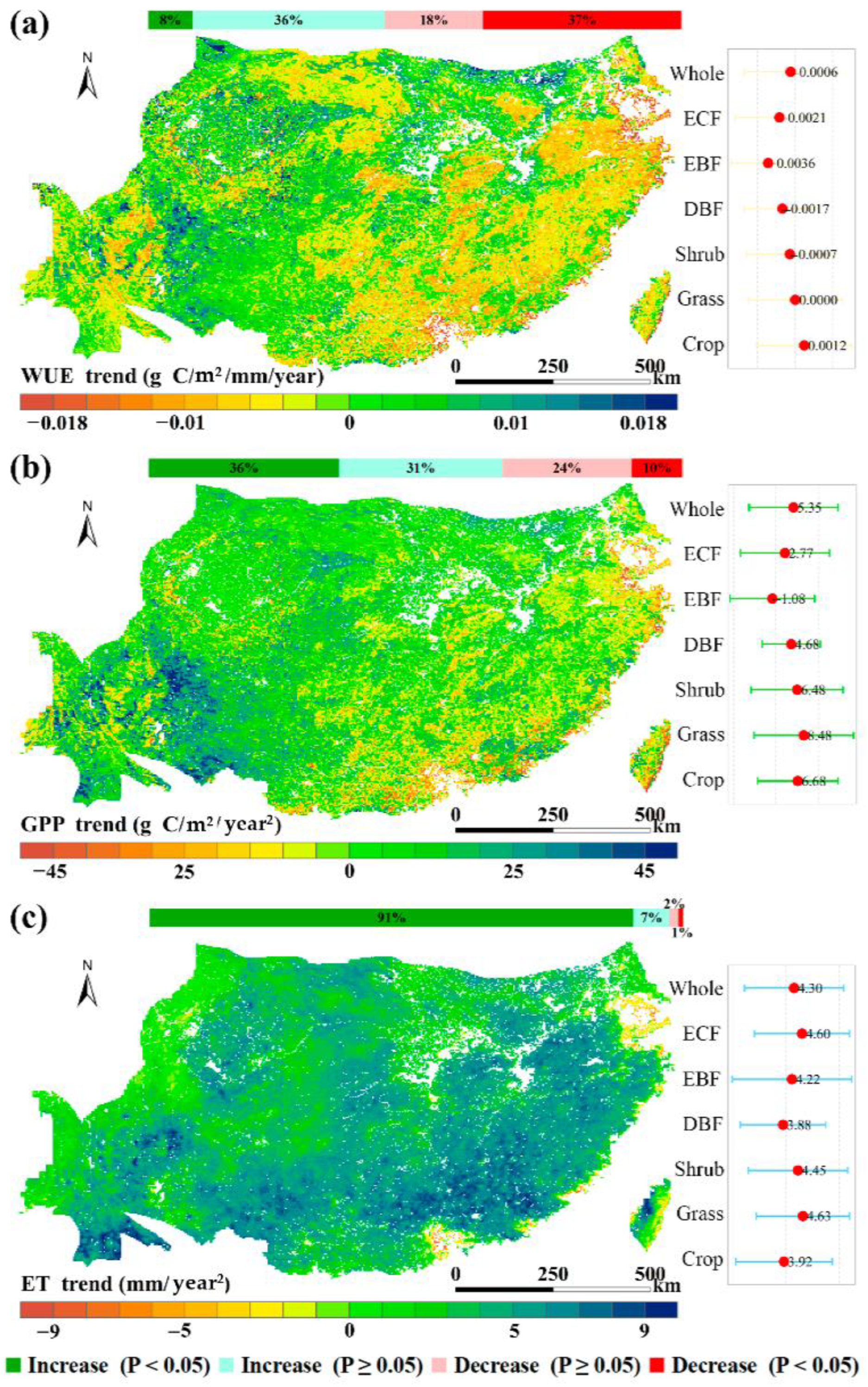
3.1. Distribution of WUE, GPP, ET, and Their Trends

The distributions of the average annual WUE, GPP, and ET in the STC from 1982 to 2018 are illustrated in Figure 1. In the entire vegetation coverage area, the annual average value of WUE ranged from 0 to 7.72 g C/m²/mm, and approximately 90% of the vegetation area had a WUE higher than 1 g C/m²/mm, with 14% of the vegetation area presenting a WUE above 2 g C/m²/mm. In the vegetated area, the annual mean GPP value ranged from 0 to 2944 g C/m²/year. The spatial distribution pattern was consistent with the annual mean WUE (Figure 1a,b). In the same area, the annual mean ET value ranged from 0 to 1703 mm/year; 51.40% of the vegetation area had an annual mean ET value higher than 1000 mm/year, and only 1% of the vegetation area had an annual mean ET value lower than 500 mm/year.

Among the six major landscapes (Figure 1), EBF had the highest annual average WUE at 1.89 g C/m²/mm, followed by DBF at 1.74 g C/m²/mm, and ECF at 1.70 g C/m²/mm. Croplands had the lowest annual average WUE of 1.33 g C/m²/mm. The annual mean GPP was similar to that of the WUE in different landscape types, with EBF having the highest annual mean GPP (1954 g C/m²/year) and cropland having the lowest (1303 g C/m²/year). The annual mean ET values in different landscapes were almost consistent between 910 and 1050 mm/year.

The spatial distributions of the variations in annual WUE, GPP, and ET from 1982 to 2018 are illustrated in Figure 2. Trends for WUE ranged between −0.23 and 0.14 g C/m²/mm/year. The changing trends in GPP and WUE showed similar spatial distribution patterns, but were quite different from those of ET (Figure 2c). For the six landscapes, WUE decreased over the study period, with the strongest downward trend in EBF (−0.0037 g C/m²/mm/year) and a weaker trend in grassland (−0.0001 g C/m²/mm/year). In addition, cropland showed an increasing trend (0.0007 g C/m²/mm/year). The trend of GPP was between −110 and 95 g C/m²/year² (Figure 2b), with the GPP of DBF, ECF, shrub, grassland, and cropland increasing to varying degrees, and the GPP of EBF decreasing slightly. The trend of ET was between −10 and 11 mm/year² (Figure 2c). At the same time, the change in ET showed an increasing trend for all landscapes.

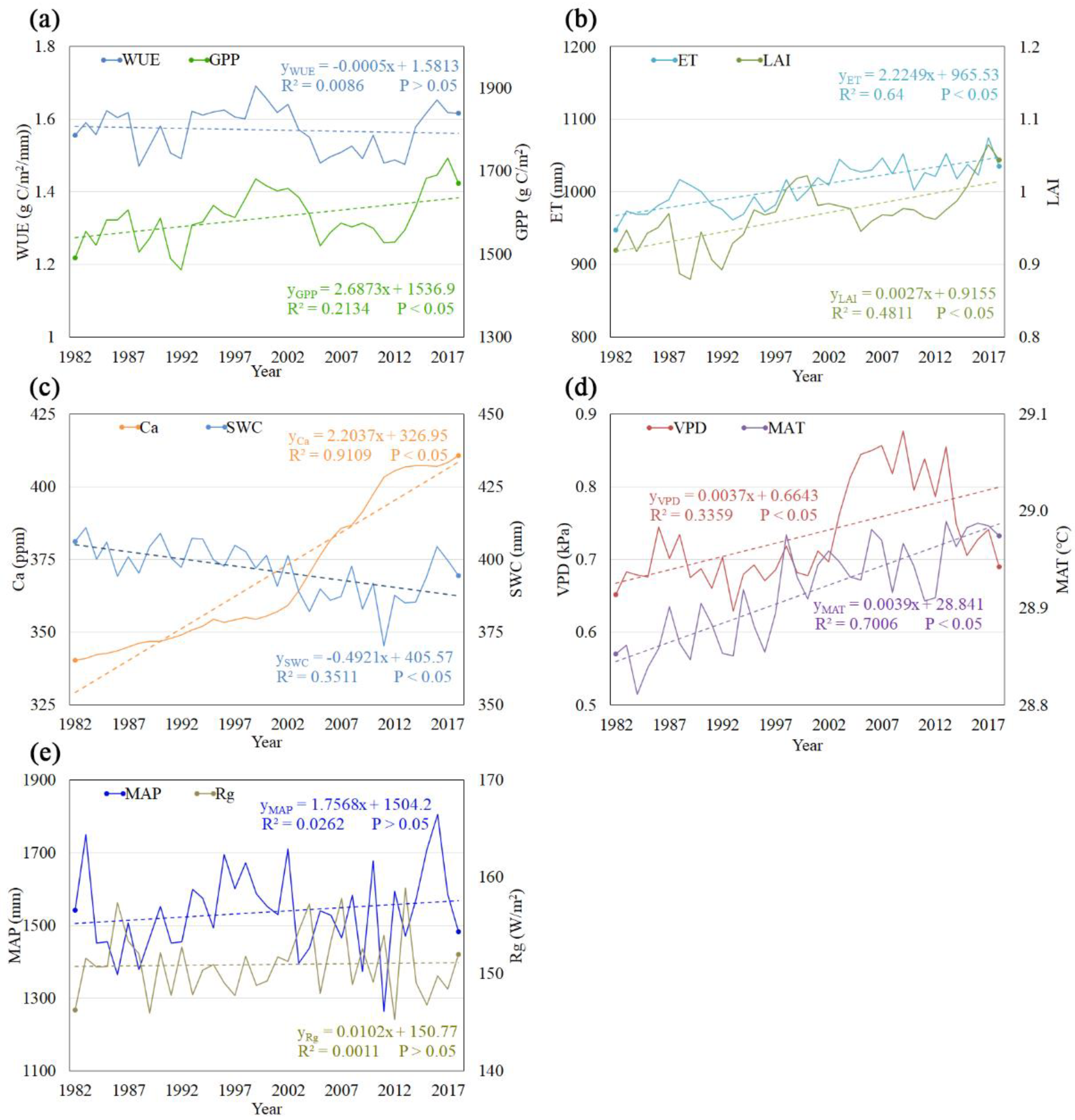
3.2. Relationships of WUE Trend with Driving Factor Trends

The ridge regression coefficient was used to represent the effects of GPP and ET on WUE trends. Among the six major landscape types in the STC, GPP had a positive effect on WUE while ET had a negative effect. The effect of GPP on the trend of WUE was higher than that of ET, and the gap between GPP and ET was largest in cropland (

Table 1. Ridge regression coefficients of GPP and ET for the annual WUE trends for different landscapes in subtropical China.

	Whole	ECF	EBF	DBF	Shrub	Grassland	Cropland
GPP	0.17	0.15	0.14	0.12	0.15	0.16	0.19
ET	−0.06	−0.06	−0.07	−0.07	−0.06	−0.06	−0.05

).

The effects of climate change, vegetation growth, and elevated atmospheric CO₂ concentration (i.e., MAT, MAP, Rg, SWC, VPD, Ca, and LAI) on interannual variations in WUE from 1982 to 2018 are shown in Figure 3. In the STC, MAT, LAI, Rg, and MAP had positive direct effects on the WUE trend; among them, the direct effects of MAT (α = 0.49) and LAI (α = 0.42) were the strongest, while those of Rg (α = 0.10) and MAP (α = 0.02) were the weakest. In contrast, VPD (α = −0.20) and Ca (α = −0.03) had negative direct effects on WUE. The direct effect of SWC on WUE was also relatively weak (Figure 3a). The spatial distribution of the direct effects of the drivers is shown in Figure S4.

The total effect of the driver on the WUE trend is the sum of the direct effect and the cumulative indirect effects. The total effect of LAI on the WUE trend was very strong because the cumulative indirect and direct effects were both positive. LAI, MAT, and Ca had a strong positive correlation, and both LAI and MAT had a strong positive direct effect on the WUE trend; therefore, Ca had a strong positive indirect effect on the WUE trend through LAI and MAT. The opposite direct and indirect effects offset each other and resulted in a total positive effect of Ca. There was a positive correlation between VPD and MAT, Rg, and LAI; the cumulative positive indirect effect resulted in a positive total effect of VPD on the WUE trend. The direct effect of SWC on the WUE trend was weak, and the total effect of SWC on the WUE trend was mainly due to the cumulative indirect effect. There was a positive correlation between MAT and LAI, VPD; however, LAI and VPD had opposite direct effects on the WUE trend. The opposite indirect effects by LAI and VPD offset each other and resulted in a weaker total effect of MAT. The characteristics of MAP were consistent with those of Rg, and the total effect was mainly driven by the direct effect. Among different landscape types, the magnitudes and directions of the direct and indirect effects of drivers on WUE trends were similar to those of the area (i.e., whole; Figure 3a).

3.3. Attribution of Variation in WUE

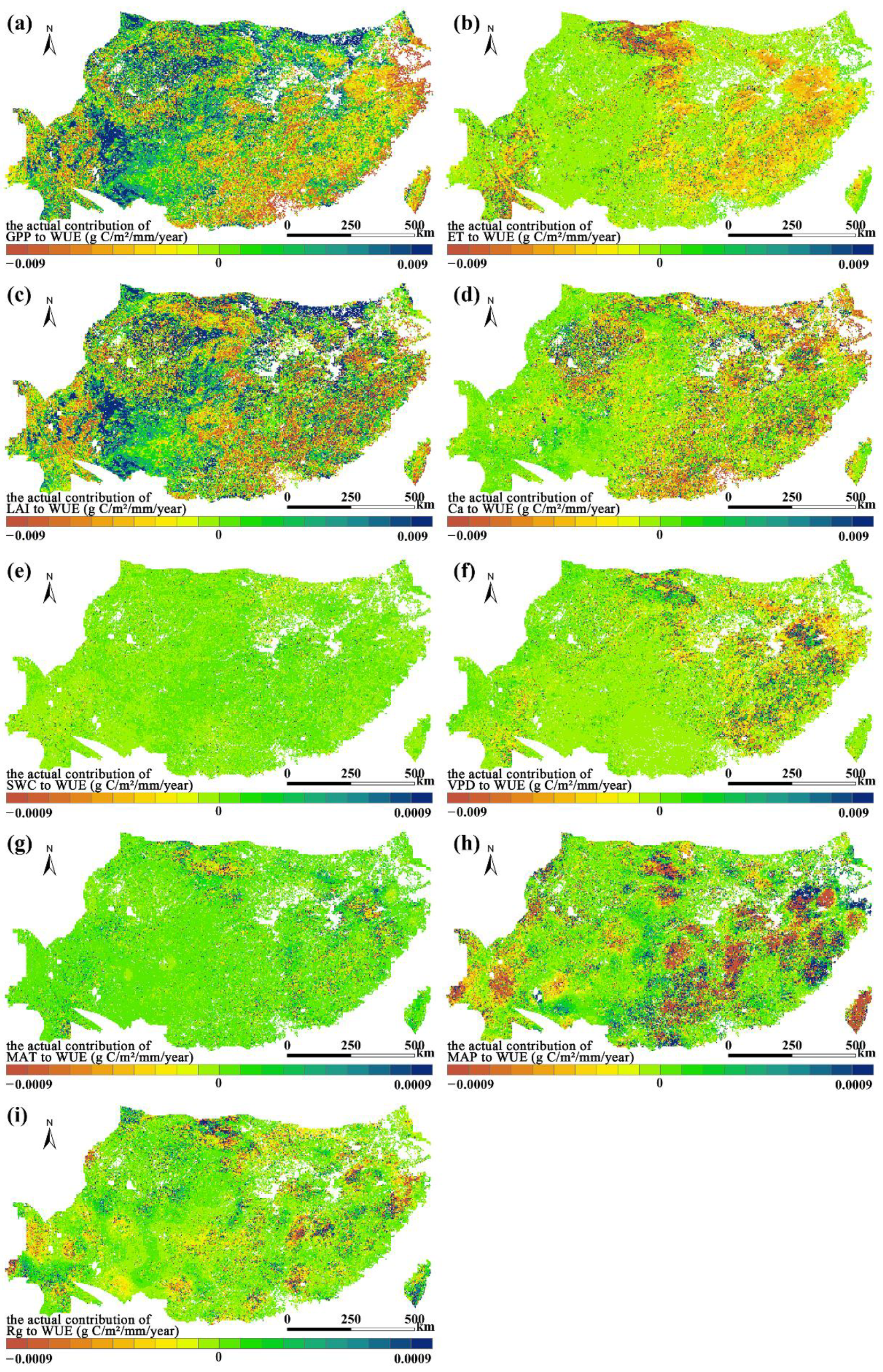
3.3.1. Actual Contribution of Driving Factors

The spatial patterns of the actual contributions of GPP and ET to the variation in WUE (Figure 4a,b, respectively) were as follows: for the whole region, GPP change contributed to a WUE change of 0.0014 g C/m²/mm/year, while ET contributed to a WUE change of −0.0020 g C/m²/mm/year. These findings suggest that the increase and decrease in WUE are mainly affected by changes in GPP and ET, respectively. Among the six major landscapes, ET changes negatively contributed to the WUE of all landscapes while GPP changes positively contributed to the WUE of DBF, grassland, and cropland but negatively contributed to the WUE of ECF, EBF, and shrubland (

Table 2. Actual contributions of GPP, ET, climate change, LAI, and Ca to annual WUE trends for different landscapes in subtropical China (×10⁻⁴ g C/m²/mm/year).

	Whole	ECF	EBF	DBF	Shrub	Grassland	Cropland
GPP	14	−9	−10	5	−1	105	18
ET	−20	−12	−26	−22	−6	−105	−6
LAI	26	−8	−45	36	−15	70	78
Ca	−21	−5	15	−24	−21	−43	−32
SWC	0	0	−1	0	0	0	0
VPD	−12	−7	5	−29	29	−20	−41
MAT	2	0	2	2	0	1	4
MAP	−1	−2	−13	−4	−1	−2	2
Rg	0	1	1	2	1	−7	0

).

The actual contribution maps of the climate change, vegetation growth, and elevated atmospheric CO2 concentration (i.e., MAT, MAP, Rg, SWC, VPD, Ca, and LAI) for the WUE trend from 1982 to 2018 are shown in Figure 4. Overall, the changes in LAI and MAT contributed to increases in WUE (Table 2) of 0.0026 g C/m²/mm/year and 0.0002 g C/m²/mm/year in WUE, respectively. Moreover, changes in Ca, VPD, and MAP caused decreases in WUE of 0.0021 g C/m²/mm/year, 0.0012 g C/m2/mm/year, and 0.0001 g C/m²/mm/year, respectively, while changes in SWC and Rg contributed weakly to the WUE trend (Table 2).

The actual contributions of climate change, LAI changes, and Ca to the WUE trends of different landscape types in the STC show that LAI changes made the largest contribution to the EBF, DBF, and cropland WUE trends at −0.0045 g C/m²/mm/year, 0.0036 g C/m²/mm/year, and 0.0078 g C/m²/mm/year, respectively. For grasslands, Ca had the largest contribution to the WUE trend at −0.0043 g C/m²/mm/year, while for shrubland, VPD contributed the most to the WUE trend at 0.0029 g C/m²/mm/year. In ECF, LAI changes, Ca, and VPD contributed equally to the WUE trends. The actual contributions of the drivers in different landscape types to WUE trends are listed in Table 2.

3.3.2. Relative Contributions of Driving Factors

The dominant factor underlying the WUE trends for each pixel was determined by the relative contribution of the driver to the WUE trend. Figure 5a,b show the WUE trend for the GPP-dominated area, which accounted for 79.98% of the total area. In different landscape types, the proportion of the area dominated by GPP exceeded 60%, indicating that the trend of WUE in most areas of the STC was dominated by changes in GPP.

The relative contribution maps of the three drivers (i.e., climate change, vegetation growth, and elevated atmospheric CO₂ concentration) for the WUE trend during 1982– 2018 are shown in Figure 5c. Figure 5d shows the proportions of areas dominated by different driving factors. In the STC, LAI variation alone dominated the WUE trend in 58.46% of the area. Among the six major landscapes, dominant areas were also all over 50%, indicating that LAI variation is the primary factor in WUE trends across all landscapes. Ca and climate change dominated the WUE trends of 13.79% and 13.43% of the area, respectively. In cropland, the area where elevated Ca was dominant exceeded that of climate variables, indicating that Ca is a more important driver of WUE trends in cropland, while in natural landscapes (i.e., those other than cropland), the area where climate variables were dominant exceeded that of elevated Ca, indicating that climate variables are more important drivers of WUE trends in natural landscapes. Meanwhile, the single-factor categories (Cli, LAI change, or Ca) had a limited ability to control the spatiotemporal dynamics of WUE (controlling the area ratio according to the quantified dominant factor). Excluding the single dominant factors, the coupled effect of LAI change and Ca (Figure 5d) was an important driver of WUE change that dominated 3.61% of the area, while the coupled effect of Cli and LAI change was an important driver that dominated 2.92% of the area. In addition, the proportion of the balanced influence of the three factors accounted for 7.12% of the WUE trend, and the influence of the combined factors was evenly distributed among the various landscapes.

4. Discussion

4.1. WUE Changes in Different Vegetation Types

Using the GPP and ET of GLASS, this study identified an annual average WUE of 1.57 g C/m²/mm for ecosystems in the STC. This value is close to WUE values reported by Wang and Zhao et al. for ecosystems in Southwest China, which belongs to the STC [40,41], which were slightly lower than the those of ecosystems in the mixed subtropical and tropical regions of South Asia [25,42], and higher than those of ecosystems in temperate regions, such as the Loess Plateau of China [43]. From the perspective of different landscape types, EBF had the highest WUE, followed by DBF and ECF; shrubland and grassland had consistent WUE, while cropland had the lowest WUE. Differences in WUE among landscape types may be due to differences in carbon uptake and water consumption [44]. In the STC, the GPP of EBF was much higher than that of other landscapes, and the gap in ET between different landscapes was smaller; therefore, the WUE of EBF was the largest. The GPP of DBF had obvious seasonal variation; therefore, the WUE of this landscape on an annual scale was not high. Previous studies have generally shown that the WUE of forest ecosystems is higher than that of grassland ecosystems [35], which is consistent with our findings. Woodlands have denser canopies and more developed root systems and thus can intercept and utilize a greater quantity of solar radiation and soil moisture, thereby contributing to greater ecosystem WUE and plant growth [35,45].

From 1982 to 2018, global ecosystems generally experienced climate warming. Based on increases in regional precipitation combined with the influence of human activities, such as returning farmland to forests, the ET and GPP in most regions of China have shown upward trends to varying degrees [46,47]. A comparison of the trends of the normalized GPP and ET is shown in Figure S6. The upward trend of ET, which was slightly higher than that of GPP, was the direct cause of the decline in the overall WUE of the STC. Among the different landscape types, the ET of ECF, DBF, and shrubland showed an upward trend that slightly exceeded that of GPP, leading to a decline in WUE; moreover, the ET and GPP of EBF showed upward and downward trends, respectively, resulting in the most significant decline in WUE. Second, the ET and GPP of grassland had similar upward trends, which led to a relatively stable WUE, and the GPP of cropland had a higher upward trend than ET. Therefore, cropland WUE had an upward trend. Huang et al. (2016) and Ji et al. (2021) conducted global WUE studies from 1982 to the present, and showed a decreasing trend of WUE in the STC [48,49], which is consistent with the findings of this study. While afforestation can slow climate warming by sequestering carbon, the decline in WUE means that on top of that, a higher proportion of water needs to be consumed to maintain the same level of vegetation carbon sequestration. Therefore, the planning and management of ecological protection and restoration requires more thinking and trade-offs between water resources and hydrology [50].

4.2. Response of WUE to the Driving Factors

Previous studies have demonstrated that ecosystem WUE is affected by both biotic factors, including vegetation growth, and abiotic factors, including the climatic environment [19,20,51]. The impact of climatic variables on WUE changes has been extensively demonstrated. Warming affects vegetation productivity by extending the growing season in favor of greenery. The ET rate remains constant or increases gradually owing to greenery [8,52]. Therefore, the warming of the STC has a positive effect on the WUE. An increase in solar radiation will lead to an increase in GPP, and radiation is positively correlated with canopy conductance and transpiration [52,53]. In the STC, changes in solar radiation stimulated GPP more significantly than ET, which ultimately led to changes in WUE. Precipitation is the dominant factor in surface ecohydrological processes. Increased precipitation promotes vegetation growth and surface evapotranspiration (both vegetation transpiration and surface evaporation). The response of vegetation to changes in precipitation may exhibit a threshold effect; when precipitation exceeds a certain threshold, the GPP’s response to increased rainfall is weakened [54], Thus, in the humid STC, fluctuating increases in rainfall have a negative impact on WUE. In humid areas, moisture is usually not a limiting factor for vegetation growth. Other studies have shown that SWC is not a major driver of humid ecosystem GPP and ET [35,55]. The effect of VPD on WUE is well-known, with elevated VPD leading to decreased WUE, which is also consistent with previous studies [27]. Elevated VPD can lead to a decrease in the stomatal conductance of vegetation, resulting in a decrease in the photosynthetic rate and GPP. Simultaneously, reduced stomatal conductance reduces ET. Studies have shown that under high humidity conditions, GPP is more sensitive to VPD changes than ET, resulting in a negative impact of VPD increases on WUE [56] (Figure 6).

LAI, as an indicator reflecting the biological characteristics of vegetation affected by climate change and human activities, varies in different landscapes. LAI changes affect the rate of absorption of photosynthetically active radiation and the allocation of radiation among latent and sensible heat fluxes. Many previous analyses have demonstrated that LAI shows a strong positive influence on GPP, whereas LAI shows a greater positive impact on seasonal ET but a weaker effect on long-term ET [56,57]. Thus, on an interannual scale, the impact on GPP by LAI exceeds that on ET [58]. Several studies have also reported a positive relationship between LAI and ecosystem WUE trends [59,60]. In the STC, strong spatial heterogeneity was observed in the contribution of LAI variations to the WUE trend due to the LAI trend and the spatial heterogeneity of WUE sensitivity to LAI.

Elevated atmospheric CO₂ concentration directly affects photosynthesis (i.e., the fertilization effect of increased CO₂) by raising the CO₂ concentration gradient between cells and leaf surfaces [27,60]; moreover, an increase in the concentration of CO₂ will impact the stomatal conductance of the surface by altering the number, shape, and density of stomata [19]. In addition, when leaf stomatal CO₂ uptake rate reaches a level of saturation, there may be a reduction in transpiration due to decreases in the diameter of leaf stomata. These twin processes can result in a reduction in transpiration while vegetation productivity is maintained or improved, thereby increasing WUE. However, a higher CO₂ concentration over a long time is also expected to increase the effective evaporation area of the leaf and surface, which can increase the total evaporation at the ecosystem level [61]. In areas with high CO₂ concentrations and abundant water resources, the effect of an elevated CO₂ concentration on water transpiration may be greater than that of CO₂ assimilation [47]. In terms of direct effects, elevated CO₂ concentrations negatively impact WUE in the STC.

The contributions of drivers to the WUE trends depend on WUE sensitivity to these drivers and to changing trends of the variables themselves. WUE showed the highest sensitivity to LAI, and the change was significant; thus, LAI is the main driver of changes in WUE. The elevated atmospheric CO₂ concentration represents an important driver of changes in WUE of the STC owing to its significant change trend.

4.3. Limitations and Future Improvements

The data used in this study were obtained from satellite remote-sensed products, which typically suffer from a relatively low spatial resolution. Although we used eddy covariance data from flux towers to validate the GPP and ET results, owing to the limitations of field monitoring data, unavoidable uncertainties were observed in our validation process. In the future, further comparison and optimization should be carried out in combination with analyses of more monitoring data. Although the WUE trend in the study area contained some insignificant pixels, to fully analyze the contribution of the driving factors of vegetation coverage to the WUE trend in the STC, performing statistical analyses on all pixels may introduce certain errors. In future research, we will strive to pursue both the stability of the trend and integrity of the study area. In this study, both vegetation growth and elevated Ca were affected by human activity. However, the impacts of human activities differ and vary in different landscapes, and identifying a surrogate index that represents various human activities is difficult; therefore, regression analysis alone cannot determine the contribution of anthropogenic activities to changes in WUE. Accurately assessing the impact of human activities on ecosystems remains a focus of future research. Although this study identified the indirect effects of driving factors on WUE trends, an effective method of quantifying the indirect contribution has not been developed. Therefore, the contribution rate is still estimated based on the trends and direct effects of the variables, which may lead to an underestimation of the contribution of climate change. It is expected that the estimation method for indirect contributions will be improved in future research.

5. Conclusions

This study investigated the spatiotemporal characteristics of WUE and driving factors in the STC from 1982 to 2018. The main results are as follows. (1) The annual average WUE of the STC was 1.57 g C/m²/mm, and the annual average WUE of woodland was slightly higher than that of grassland and cropland. Meanwhile, from 1982 to 2018, the annual cropland WUE showed an upward trend while the annual grassland WUE trend was relatively stable. The annual WUE of all other landscape types showed a downward trend. (2). MAT and LAI had strong positive direct effects on WUE, while VPD showed a strong negative direct effect on WUE. In addition, the total effect of LAI on the WUE trend was very strong because both the indirect and direct effects were positive. The opposing indirect and direct effects cancelled each other out, resulting in the total effect of Ca and VPD on WUE trends being positive. The influence of SWC on WUE trends is mainly through indirect effects. The influence of MAT, MAP, and Rg on the WUE trend is mainly through direct effects, because the opposite indirect effects of their different paths are offset. (3). LAI had a major contribution to the increasing trend of WUE, whereas Ca and VPD had a major contribution to the decreasing trend of WUE. LAI was the primary driving factor of WUE change in the STC and dominated WUE changes in more than 50% of the total area. Ca and VPD were also important driving factors, while other drivers contributed less to the WUE trend. This study deepens our understanding of the impact of changes in the climatic environment and biological factors of vegetation on the annual variation in WUE. These findings can be used to guide ecological rehabilitation and management under a future changing climate in subtropical regions.

References

1. Baodi, D.; Mengyu, L.; Hongbo, S.; Quanqi, L.; Lei, S.; Feng, D.; Zhengbin, Z. Investigation on the relationship between leaf water use efficiency and physio-biochemical traits of winter wheat under rained condition. Colloids Surf. B Biointerfaces 2008, 62, 280–287. [Google Scholar] [CrossRef]
2. Frank, D.C.; Poulter, B.; Saurer, M.; Esper, J.; Huntingford, C.; Helle, G.; Treydte, K.; Zimmermann, N.E.; Schleser, G.H.; Ahlström, A.; et al. Water-use efficiency and transpiration across European forests during the Anthropocene. Nat. Clim. Change 2015, 5, 579–583. [Google Scholar] [CrossRef]
3. Tian, H.; Chen, G.; Liu, M.; Zhang, C.; Sun, G.; Lu, C.; Xu, X.; Ren, W.; Pan, S.; Chappelka, A. Model estimates of net primary productivity, evapotranspiration, and water use efficiency in the terrestrial ecosystems of the southern United States during 1895–2007. For. Ecol. Manag. 2010, 259, 1311–1327. [Google Scholar] [CrossRef]
4. Keenan, T.F.; Hollinger, D.Y.; Bohrer, G.; Dragoni, D.; Munger, J.W.; Schmid, H.P.; Richardson, A.D. Increase in forest water-use efficiency as atmospheric carbon dioxide concentrations rise. Nature 2013, 499, 324–327. [Google Scholar] [CrossRef]
5. Yang, L.; Feng, Q.; Wen, X.; Barzegar, R.; Adamowski, J.F.; Zhu, M.; Yin, Z. Contributions of climate, elevated atmospheric CO2 concentration and land surface changes to variation in water use efficiency in Northwest China. Catena 2022, 213, 106220. [Google Scholar] [CrossRef]
6. Cai, W.; Ullah, S.; Yan, L.; Lin, Y. Remote Sensing of Ecosystem Water Use Efficiency: A Review of Direct and Indirect Estimation Methods. Remote Sens. 2021, 13, 2393. [Google Scholar] [CrossRef]
7. Liu, W.; Mo, X.; Liu, S.; Lin, Z.; Lv, C. Attributing the changes of grass growth, water consumed and water use efficiency over the Tibetan Plateau. J. Hydrol. 2021, 598, 126464. [Google Scholar] [CrossRef]
8. Xie, S.; Mo, X.; Hu, S.; Liu, S. Contributions of climate change, elevated atmospheric CO2 and human activities to ET and GPP trends in the Three-North Region of China. Agric. For. Meteorol. 2020, 295, 108183. [Google Scholar] [CrossRef]
9. Aboelsoud, H.M.; AbdelRahman, M.A.E.; Kheir, A.M.S.; Eid, M.S.M.; Ammar, K.A.; Khalifa, T.H.; Scopa, A. Quantitative Estimation of Saline-Soil Amelioration Using Remote-Sensing Indices in Arid Land for Better Management. Land 2022, 11, 1041. [Google Scholar] [CrossRef]
10. Jin, Z.; Liang, W.; Yang, Y.; Zhang, W.; Yan, J.; Chen, X.; Li, S.; Mo, X. Separating Vegetation Greening and Climate Change Controls on Evapotranspiration trend over the Loess Plateau. Sci. Rep. 2017, 7, 8191. [Google Scholar] [CrossRef]
11. Yang, S.; Zhang, J.; Zhang, S.; Wang, J.; Bai, Y.; Yao, F.; Guo, H. The potential of remote sensing-based models on global water-use efficiency estimation: An evaluation and intercomparison of an ecosystem model (BESS) and algorithm (MODIS) using site level and upscaled eddy covariance data. Agric. For. Meteorol. 2020, 287, 107959. [Google Scholar] [CrossRef]
12. Yang, L.; Feng, Q.; Yin, Z.; Deo, R.C.; Wen, X.; Si, J.; Liu, W. Regional hydrology heterogeneity and the response to climate and land surface changes in arid alpine basin, northwest China. Catena 2020, 187, 104345. [Google Scholar] [CrossRef]
13. Wu, L.; Wang, S.; Bai, X.; Tian, Y.; Luo, G.; Wang, J.; Li, Q.; Chen, F.; Deng, Y.; Yang, Y.; et al. Climate change weakens the positive effect of human activities on karst vegetation productivity restoration in southern China. Ecol. Indic. 2020, 115, 106392. [Google Scholar] [CrossRef]
14. Zhou, S.; Yu, B.; Huang, Y.; Wang, G. Daily underlying water use efficiency for AmeriFlux sites. J. Geophys. Res. Biogeosciences 2015, 120, 887–902. [Google Scholar] [CrossRef]
15. Zhu, Z.; Piao, S.; Myneni, R.B.; Huang, M.; Zeng, Z.; Canadell, J.G.; Ciais, P.; Sitch, S.; Friedlingstein, P.; Arneth, A.; et al. Greening of the Earth and its drivers. Nat. Clim. Change 2016, 6, 791–795. [Google Scholar] [CrossRef]
16. Hungate, B.A.; Reichstein, M.; Dijkstra, P.; Johnson, D.; Hymus, G.; Tenhunen, J.; Hinkle, C.; Drake, B. Evapotranspiration and soil water content in a scrub-oak woodland under carbon dioxide enrichment. Glob. Change Biol. 2002, 8, 289–298. [Google Scholar] [CrossRef]
17. Liu, X.; Feng, X.; Fu, B. Changes in global terrestrial ecosystem water use efficiency are closely related to soil moisture. Sci. Total Environ. 2020, 698, 134165. [Google Scholar] [CrossRef]
18. Nie, C.; Huang, Y.; Zhang, S.; Yang, Y.; Zhou, S.; Lin, C.; Wang, G. Effects of soil water content on forest ecosystem water use efficiency through changes in transpiration/evapotranspiration ratio. Agric. For. Meteorol. 2021, 308–309, 108605. [Google Scholar] [CrossRef]
19. Gentine, P.; Green, J.K.; Guérin, M.; Humphrey, V.; Seneviratne, S.I.; Zhang, Y.; Zhou, S. Coupling between the terrestrial carbon and water cycles—A review. Environ. Res. Lett. 2019, 14, 83003. [Google Scholar] [CrossRef]
20. Migliavacca, M.; Musavi, T.; Mahecha, M.D.; Nelson, J.A.; Knauer, J.; Baldocchi, D.D.; Perez-Priego, O.; Christiansen, R.; Peters, J.; Anderson, K.; et al. The three major axes of terrestrial ecosystem function. Nature 2021, 598, 468–472. [Google Scholar] [CrossRef]
21. Tang, X.; Ma, M.; Ding, Z.; Xu, X.; Yao, L.; Huang, X.; Gu, Q.; Song, L. Remotely Monitoring Ecosystem Water Use Efficiency of Grassland and Cropland in China’s Arid and Semi-Arid Regions with MODIS Data. Remote Sens. 2017, 9, 616. [Google Scholar] [CrossRef]
22. Wang, Y.; Zhou, L.; Ping, X.; Jia, Q.; Li, R. Ten-year variability and environmental controls of ecosystem water use efficiency in a rainfed maize cropland in Northeast China. Field Crops Res. 2018, 226, 48–55. [Google Scholar] [CrossRef]
23. Sun, Y.; Piao, S.; Huang, M.; Ciais, P.; Zeng, Z.; Cheng, L.; Li, X.; Zhang, X.; Mao, J.; Peng, S.; et al. Global patterns and climate drivers of water-use efficiency in terrestrial ecosystems deduced from satellite-based datasets and carbon cycle models. Glob. Ecol. Biogeogr. 2016, 25, 311–323. [Google Scholar] [CrossRef]
24. Yang, S.; Zhang, J.; Han, J.; Wang, J.; Zhang, S.; Bai, Y.; Cao, D.; Xun, L.; Zheng, M.; Chen, H.; et al. Evaluating global ecosystem water use efficiency response to drought based on multi-model analysis. Sci. Total Environ. 2021, 778, 146356. [Google Scholar] [CrossRef]
25. Nandy, S.; Saranya, M.; Srinet, R. Spatio-temporal variability of water use efficiency and its drivers in major forest formations in India. Remote Sens. Environ. 2022, 269, 112791. [Google Scholar] [CrossRef]
26. Sun, H.; Bai, Y.; Lu, M.; Wang, J.; Tuo, Y.; Yan, D.; Zhang, W. Drivers of the water use efficiency changes in China during 1982-2015. Sci. Total Environ. 2021, 799, 149145. [Google Scholar] [CrossRef]
27. Zhao, F.; Wu, Y.; Ma, S.; Lei, X.; Liao, W. Increased Water Use Efficiency in China and Its Drivers During 2000–2016. Ecosystems 2022, 1–17. [Google Scholar] [CrossRef]
28. Hu, X.; Lei, H. Fifteen-year Variations of Water Use Efficiency over a Wheat-Maize Rotation Cropland in the North China Plain. Agric. For. Meteorol. 2021, 306, 108430. [Google Scholar] [CrossRef]
29. Ren, P.; Liu, Z.; Zhou, X.; Peng, C.; Xiao, J.; Wang, S.; Li, X.; Li, P. Strong controls of daily minimum temperature on the autumn photosynthetic phenology of subtropical vegetation in China. For. Ecosyst. 2021, 8, 31. [Google Scholar] [CrossRef]
30. Zhang, T.; Peng, J.; Liang, W.; Yang, Y.; Liu, Y. Spatial-temporal patterns of water use efficiency and climate controls in China’s Loess Plateau during 2000–2010. Sci. Total Environ. 2016, 565, 105–122. [Google Scholar] [CrossRef]
31. Yao, Y.; Liang, S.; Li, X.; Hong, Y.; Fisher, J.B.; Zhang, N.; Chen, J.; Cheng, J.; Zhao, S.; Zhang, X.; et al. Bayesian multimodel estimation of global terrestrial latent heat flux from eddy covariance, meteorological, and satellite observations. J. Geophys. Res. Atmos. 2014, 119, 4521–4545. [Google Scholar] [CrossRef]
32. Yuan, W.; Liu, S.; Yu, G.; Bonnefond, J.-M.; Chen, J.; Davis, K.; Desai, A.R.; Goldstein, A.H.; Gianelle, D.; Rossi, F.; et al. Global estimates of evapotranspiration and gross primary production based on MODIS and global meteorology data. Remote Sens. Environ. 2010, 114, 1416–1431. [Google Scholar] [CrossRef]
33. He, J.; Yang, K.; Tang, W.; Lu, H.; Qin, J.; Chen, Y.; Li, X. The first high-resolution meteorological forcing dataset for land process studies over China. Sci. Data 2020, 7, 25. [Google Scholar] [CrossRef] [PubMed]
34. Yang, K.; He, J.; Tang, W.; Qin, J.; Cheng, C.C.K. On downward shortwave and longwave radiations over high altitude regions: Observation and modeling in the Tibetan Plateau. Agric. For. Meteorol. 2010, 150, 38–46. [Google Scholar] [CrossRef]
35. Hu, Z.; Yu, G.; Fu, Y.; Sun, X.; Li, Y.; Shi, P.; Wang, Y.; Zheng, Z. Effects of vegetation control on ecosystem water use efficiency within and among four grassland ecosystems in China. Glob. Change Biol. 2008, 14, 1609–1619. [Google Scholar] [CrossRef]
36. Sun, S.; Song, Z.; Wu, X.; Wang, T.; Wu, Y.; Du, W.; Che, T.; Huang, C.; Zhang, X.; Ping, B.; et al. Spatio-temporal variations in water use efficiency and its drivers in China over the last three decades. Ecol. Indic. 2018, 94, 292–304. [Google Scholar] [CrossRef]
37. Wang, M.; Ding, Z.; Wu, C.; Song, L.; Ma, M.; Yu, P.; Lu, B.; Tang, X. Divergent responses of ecosystem water-use efficiency to extreme seasonal droughts in Southwest China. Sci. Total Environ. 2021, 760, 143427. [Google Scholar] [CrossRef]
38. Meng, D.; Mo, X. Assessing the effect of climate change on mean annual runoff in the Songhua River basin, China. Hydrol. Processes 2012, 26, 1050–1061. [Google Scholar] [CrossRef]
39. Xing, X.; Liu, Y.; Zhao, W.g.; Kang, D.g.; Yu, M.; Ma, X. Determination of dominant weather parameters on reference evapotranspiration by path analysis theory. Comput. Electron. Agric. 2016, 120, 10–16. [Google Scholar] [CrossRef]
40. Zhao, J.; Xu, T.; Xiao, J.; Liu, S.; Mao, K.; Song, L.; Yao, Y.; He, X.; Feng, H. Responses of Water Use Efficiency to Drought in Southwest China. Remote Sens. 2020, 12, 199. [Google Scholar] [CrossRef] [Green Version]
41. Wang, H.; Li, X.; Xiao, J.; Ma, M. Evapotranspiration components and water use efficiency from desert to alpine ecosystems in drylands. Agric. For. Meteorol. 2021, 298–299, 108283. [Google Scholar] [CrossRef]
42. Kayiranga, A.; Chen, B.; Guo, L.; Measho, S.; Hirwa, H.; Liu, S.; Bofana, J.; Sun, S.; Wang, F.; Karamage, F.; et al. Spatiotemporal variations of forest ecohydrological characteristics in the Lancang-Mekong region during 1992–2016 and 2020–2099 under different climate scenarios. Agric. For. Meteorol. 2021, 310, 108662. [Google Scholar] [CrossRef]
43. Zheng, H.; Lin, H.; Zhou, W.; Bao, H.; Zhu, X.; Jin, Z.; Song, Y.; Wang, Y.; Liu, W.; Tang, Y. Revegetation has increased ecosystem water-use efficiency during 2000–2014 in the Chinese Loess Plateau: Evidence from satellite data. Ecol. Indic. 2019, 102, 507–518. [Google Scholar] [CrossRef]
44. Gao, Y.; Zhu, X.; Yu, G.; He, N.; Wang, Q.; Tian, J. Water use efficiency threshold for terrestrial ecosystem carbon sequestration in China under afforestation. Agric. For. Meteorol. 2014, 195–196, 32–37. [Google Scholar] [CrossRef]
45. Li, G.; Chen, W.; Li, R.; Zhang, X.; Liu, J. Assessing the spatiotemporal dynamics of ecosystem water use efficiency across China and the response to natural and human activities. Ecol. Indic. 2021, 126, 107680. [Google Scholar] [CrossRef]
46. Li, H.; Wu, Y.; Liu, S.; Xiao, J. Regional contributions to interannual variability of net primary production and climatic attributions. Agric. For. Meteorol. 2021, 303, 108384. [Google Scholar] [CrossRef]
47. Tian, J.; Zhang, Y.; Zhang, X. Impacts of heterogeneous CO2 on water and carbon fluxes across the global land surface. Int. J. Digit. Earth 2021, 14, 1175–1193. [Google Scholar] [CrossRef]
48. Ji, Y.; Li, Y.; Yao, N.; Biswas, A.; Zou, Y.; Meng, Q.; Liu, F. The lagged effect and impact of soil moisture drought on terrestrial ecosystem water use efficiency. Ecol. Indic. 2021, 133, 108349. [Google Scholar] [CrossRef]
49. Huang, M.; Piao, S.; Zeng, Z.; Peng, S.; Ciais, P.; Cheng, L.; Mao, J.; Poulter, B.; Shi, X.; Yao, Y.; et al. Seasonal responses of terrestrial ecosystem water-use efficiency to climate change. Glob. Change Biol. 2016, 22, 2165–2177. [Google Scholar] [CrossRef]
50. Yang, W.; Zhao, Y.; Wang, Q.; Guan, B. Climate, CO2, and Anthropogenic Drivers of Accelerated Vegetation Greening in the Haihe River Basin. Remote Sens. 2022, 14, 268. [Google Scholar] [CrossRef]
51. Li, X.; Farooqi, T.J.A.; Jiang, C.; Liu, S.; Sun, O.J. Spatiotemporal variations in productivity and water use efficiency across a temperate forest landscape of Northeast China. For. Ecosyst. 2019, 6, 22. [Google Scholar] [CrossRef]
52. Huang, M.; Piao, S.; Sun, Y.; Ciais, P.; Cheng, L.; Mao, J.; Poulter, B.; Shi, X.; Zeng, Z.; Wang, Y. Change in terrestrial ecosystem water-use efficiency over the last three decades. Glob. Change Biol. 2015, 21, 2366–2378. [Google Scholar] [CrossRef] [PubMed]
53. Pieruschka, R.; Huber, G.; Berry, J.A. Control of transpiration by radiation. Proc. Natl. Acad. Sci. USA 2010, 107, 13372–13377. [Google Scholar] [CrossRef] [PubMed]
54. Ma, S.; Wang, L.-J.; Jiang, J.; Chu, L.; Zhang, J.-C. Threshold effect of ecosystem services in response to climate change and vegetation coverage change in the Qinghai-Tibet Plateau ecological shelter. J. Clean. Prod. 2021, 318, 128592. [Google Scholar] [CrossRef]
55. Jiang, S.; Zhao, L.; Liang, C.; Hu, X.; Yaosheng, W.; Gong, D.; Zheng, S.; Huang, Y.; He, Q.; Cui, N. Leaf- and ecosystem-scale water use efficiency and their controlling factors of a kiwifruit orchard in the humid region of Southwest China. Agric. Water Manag. 2022, 260, 107329. [Google Scholar] [CrossRef]
56. Li, Y.; Shi, H.; Zhou, L.; Eamus, D.; Huete, A.; Li, L.; Cleverly, J.; Hu, Z.; Harahap, M.; Yu, Q.; et al. Disentangling Climate and LAI Effects on Seasonal Variability in Water Use Efficiency Across Terrestrial Ecosystems in China. J. Geophys. Res. Biogeosciences 2018, 123, 2429–2443. [Google Scholar] [CrossRef]
57. Kompanizare, M.; Petrone, R.M.; Macrae, M.L.; De Haan, K.; Khomik, M. Assessment of effective LAI and water use efficiency using Eddy Covariance data. Sci. Total Environ. 2022, 802, 149628. [Google Scholar] [CrossRef]
58. Puma, M.J.; Koster, R.D.; Cook, B.I. Phenological versus meteorological controls on land-atmosphere water and carbon fluxes. J. Geophys. Res. Biogeosciences 2013, 118, 14–29. [Google Scholar] [CrossRef]
59. Cao, R.; Hu, Z.; Jiang, Z.; Yang, Y.; Zhao, W.; Wu, G.; Feng, X.; Chen, R.; Hao, G. Shifts in ecosystem water use efficiency on china’s loess plateau caused by the interaction of climatic and biotic factors over 1985–2015. Agric. For. Meteorol. 2020, 291, 108100. [Google Scholar] [CrossRef]
60. Cheng, L.; Zhang, L.; Wang, Y.P.; Canadell, J.G.; Chiew, F.H.S.; Beringer, J.; Li, L.; Miralles, D.G.; Piao, S.; Zhang, Y. Recent increases in terrestrial carbon uptake at little cost to the water cycle. Nat. Commun. 2017, 8, 110. [Google Scholar] [CrossRef] [Green Version]
61. Lemordant, L.; Gentine, P.; Swann, A.S.; Cook, B.I.; Scheff, J. Critical impact of vegetation physiology on the continental hydrologic cycle in response to increasing CO2. Proc. Natl. Acad. Sci. USA 2018, 115, 4093–4098. [Google Scholar] [CrossRef] [PubMed] [Green Version]
62. Chen, X.F.; Jiang, H.; Niu, X.D.; Zhang, J.M.; Liu, Y.L.; Fang, C.Y. Effect of seasonal high temperature and drought on carbon flux of bamboo forest ecosystem in subtropical region. Chin. J. Appl. Ecol. 2016, 27, 335–344. [Google Scholar]
63. Han, S. Productivity Estimation of the Poplar Plantations on the Beaches in Middle and Lower Reaches of Yangtze River Using Eddy Correlation Measurement; Chinese Academy of Forestry: Beijing, China, 2008. [Google Scholar]
64. Rao, Z.; Liu, X.; Wang, R. Characteristics and impact factors of surface fluxesin Poyang Lake area. Meteorol. Disaster Res. Res. 2021, 44, 25–33. [Google Scholar]
65. Sun, H. The Study on Characteristics of Carbon and Water Fluxes and Energy Fluxes in Mixed Evergreen and Deciduous Broad-Leaved Forest in Tianmu Mountain. Master’s Thesis, Zhejiang A&F University, Hangzhou, China, 2017. [Google Scholar]
66. Wang, Z. Energy Balance and Water Vapor Flux of Snail Control and Schistosomiasis Prevention Forest Ecosystem in the Yangtze River Beach Land; Chinese Academy of Forestry: Beijing, China, 2008. [Google Scholar]
67. Zhao, Z. A Study on Carbon Flux between Chinese Fir Plantations and Atmosphere in Subtropical Belts; Central South University of Forestry and Technology: Changsha, China, 2011. [Google Scholar]
Figure 1. Spatial patterns of (a) mean annual water use efficiency (WUE), (b) Gross Primary Productivity (GPP), and (c) evapotranspiration (ET) in subtropical China. The right insets indicate the mean annual WUE, GPP, and ET of different landscapes, with whiskers indicating the standard deviations of all grid cell values. Other abbreviations: ECF, evergreen coniferous forest; EBF, evergreen broadleaf forest; DBF, deciduous broadleaf forest.
Remotesensing 14 04296 g001
Figure 2. Spatial patterns of interannual trends in (a) WUE, (b) GPP, and (c) ET in subtropical China. The top insets indicate the frequencies of significances; spatial pattern of significances is shown in Figure S2. The right insets indicate the interannual trends of WUE, GPP, and ET of different landscapes, with whiskers indicating the standard deviation of all grid cell values.
Remotesensing 14 04296 g002
Figure 3. Path diagrams between climate variables (average annual temperature (MAT), annual accumulated precipitation (MAP), and annual solar radiation (Rg), soil water content (SWC), vapor pressure deficit (VPD)), leaf area index (LAI), and elevated atmospheric CO2 (Ca), and WUE in the study area. Numbers on arrows between each factor and WUE represent direct effects, and numbers in parentheses represent total effects. Numbers on arrows between every two factors represent correlation coefficients. (a) Whole of the study area, (b) ECF, (c) EBF, (d) DBF, (e) shrub, (f) grassland, (g) cropland. R2 values beside the response variables represent the variance explained by the environmental factors and the constructed relationships. (α indicates direct effect and β indicates total effect.)
Remotesensing 14 04296 g003
Figure 4. Spatial variations in the actual contribution of (a) GPP, (b) ET (c) LAI, (d) Ca, (e) SWC, (f) VPD, (g) MAT, (h) MAP, and (i) Rg to WUE in the subtropical region of China (STC).
Remotesensing 14 04296 g004
Figure 5. Relative contributions of different driving factors to annual WUE trends based on pixel statistics. (a) Spatial patterns of the relative contributions of GPP and ET to WUE trends. (b) Controlling area ratios of GPP and ET for WUE trends. (c) Spatial patterns of the relative contributions of climate change (Cli), LAI, and Ca to WUE trends. (d) Controlling area ratios of the dominant drivers for WUE trends. The combinations of Cli, LAI, and Ca indicate that the coupled impacts of different drivers dominate WUE trends; “other” indicates the equilibrium impact of Cli, LAI, and Ca.
Remotesensing 14 04296 g005
Figure 6. Time series of annual (a) WUE and GPP, (b) ET and LAI, (c) Ca and SWC, (d) VPD and MAT, and (e) MAP and Rg in the STC.
Remotesensing 14 04296 g006