


A Fully Unsupervised Machine Learning Framework for Algal Bloom Forecasting in Inland Waters Using MODIS Time Series and Climatic Products

 ,
,  , , and
Abstract
:1. Introduction
- (i)
- A fully unsupervised learning methodology, designed to characterize, detect and predict algal blooms as time-varying anomalous events in wetland areas.
- (ii)
- The proposed approach is modular, i.e., it can be integrated with any classification model in addition to those presented in our formalization.
- (iii)
- A conceptual formalization that can be extended to other environmental issues besides inland water anomaly detection for algal blooms.
2. Methods
2.1. Machine Learning Models
2.2. Algal Bloom Detection via Spectral Index Thresholding
2.3. Characterizing and Forecasting an Algal Bloom as an Anomalous Event
2.3.1. Conceptual Formalization
2.3.2. Implementation Details and Parametrization
- Spectral Indices and Thresholds: In order to appropriately select the best set of thresholds for the spectral indices, we followed the methods of [37,42,44,45] to take the values established in these studies.Although different thresholds may result in more accurate outputs for certain study areas, the authors in [37,42,44,45] verified that the variations were minimal for a multitude of areas analyzed. Therefore, we opted to take the pre-established thresholds given in [37,42,44,45] to drive our method, but with the advantage of keeping them as free parameters in our implementation, making the method flexible enough to meet the requirements of other study areas and applications of interest.
- Model Parameter Tuning: The selection of suitable hyperparameters for each classification method (Section 2.1) was conducted by applying the randomized grid search procedure [58,59,60] with a five-fold cross-validation. The hyperparameter space-search taken for the LSTM model comprised , , . Hyperparameters related to the RF method ranged as part of the following sets: , , , and . Regarding the SVM method, the examined hyperparameters varied as follows: and .
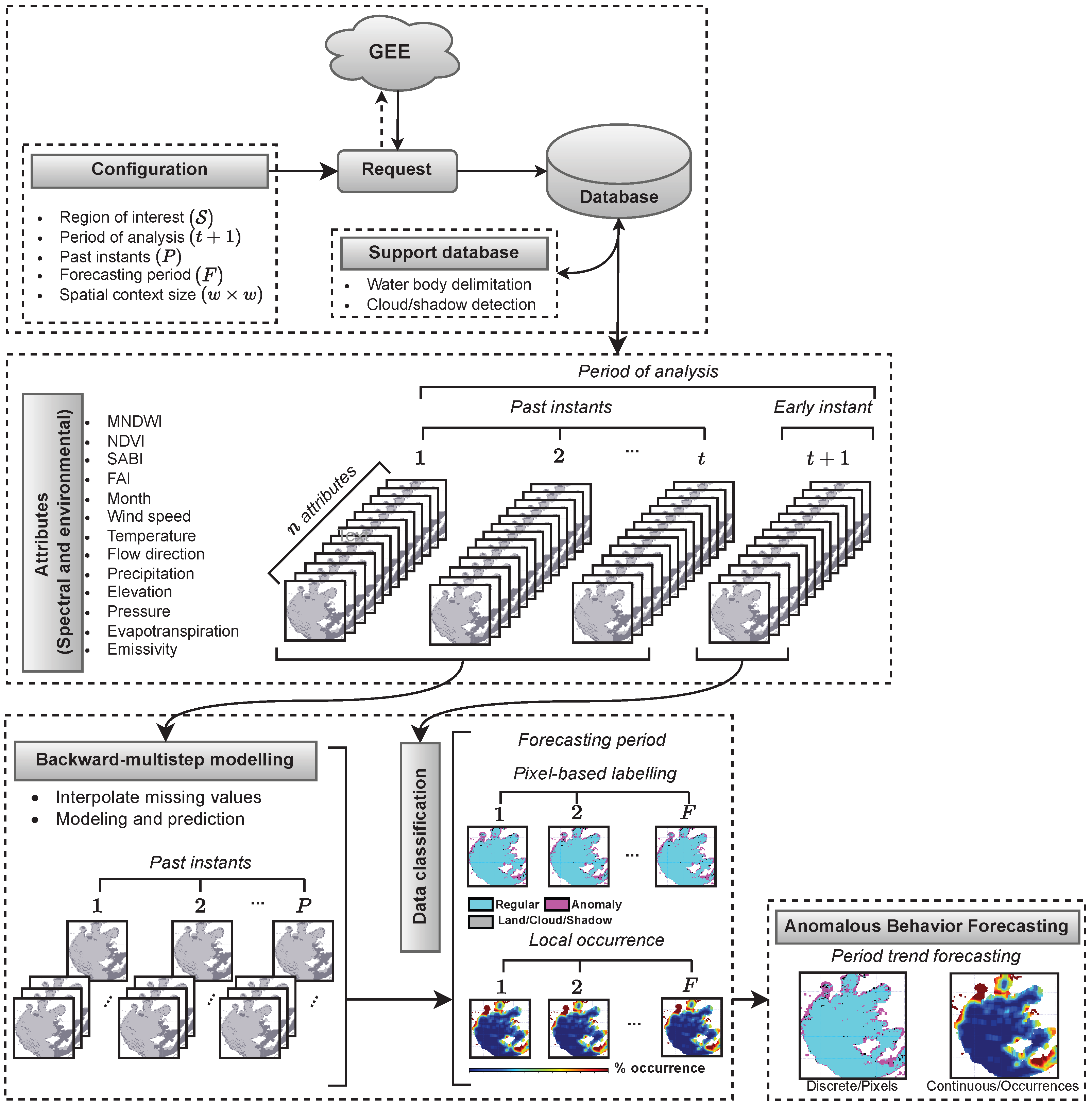
- Support Database: This database comprised the water body spatial boundaries and the occurrences of cloud/shadow during the period of analysis. Concerning water body identification, we employed the “water_mask” sub-product from MODIS (MOD44W.006/“Terra Land Water Mask”) to deliver water surface mapping with 250 m spatial resolution. Furthermore, bitwise operations were applied on the “state_1km” sub-product to detect the presence of clouds and shadows.
- Period of Analysis: This consisted of an image time series used as input data to train a machine learning model in our ABF framework. Depending on the availability of data for each study area, we were able to take different “periods of analysis” when applying our methodology. Since the period of analysis used to train the predictive models may influence the outputs, we ran an extensive battery of tests to select the most suitable training window: 180 days. More specifically, we used the following periods when performing our experimental tests: 30, 60, 90, 180, 365, 730 and 1825 days.
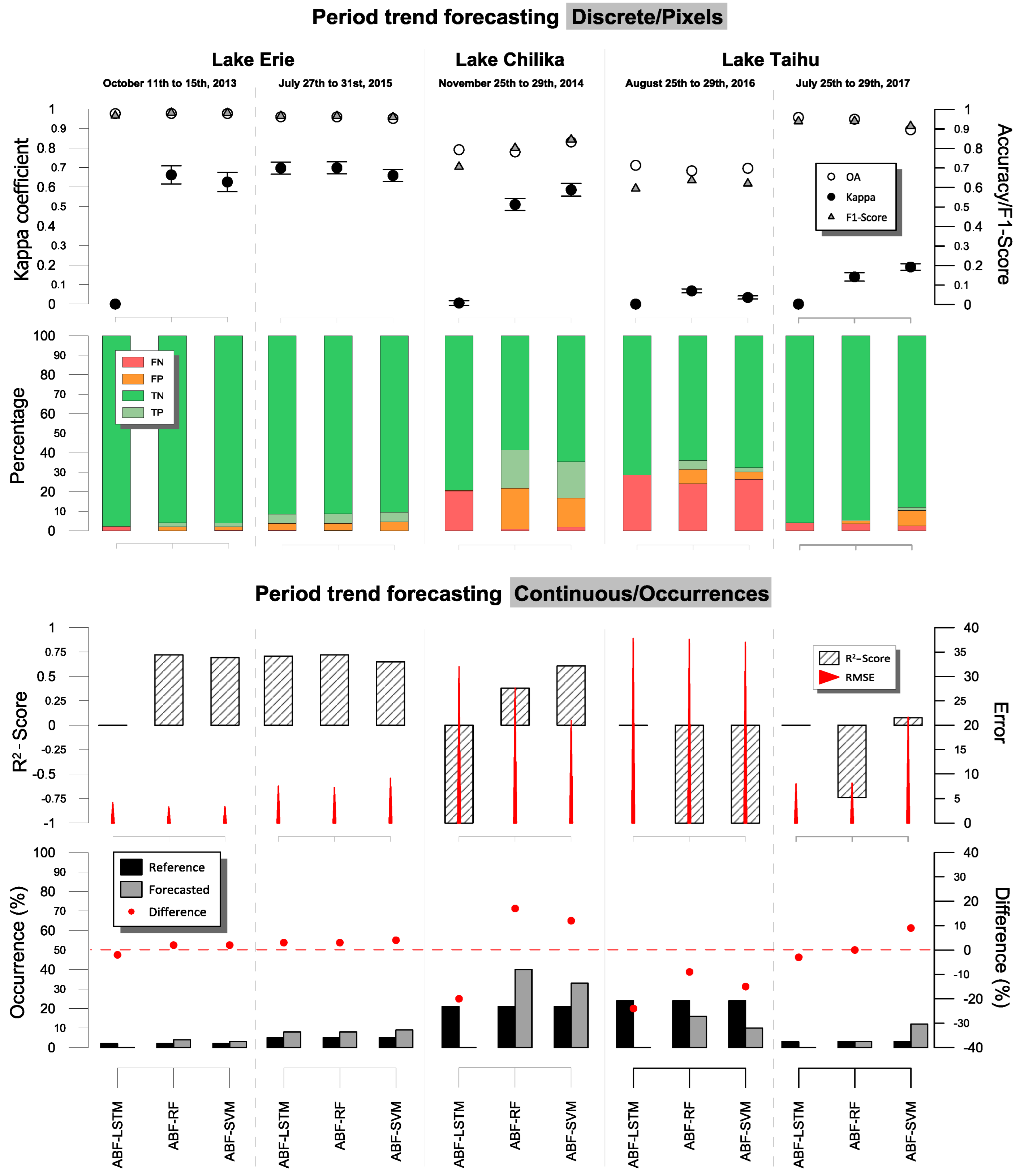
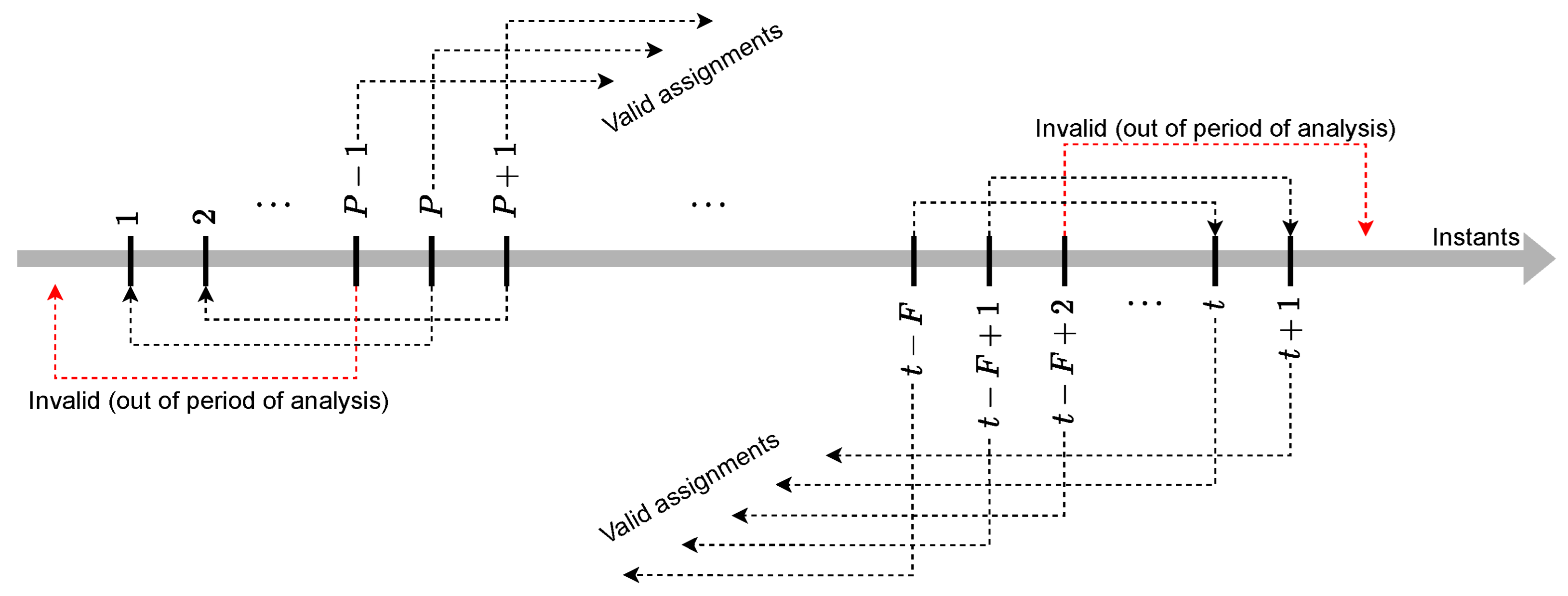
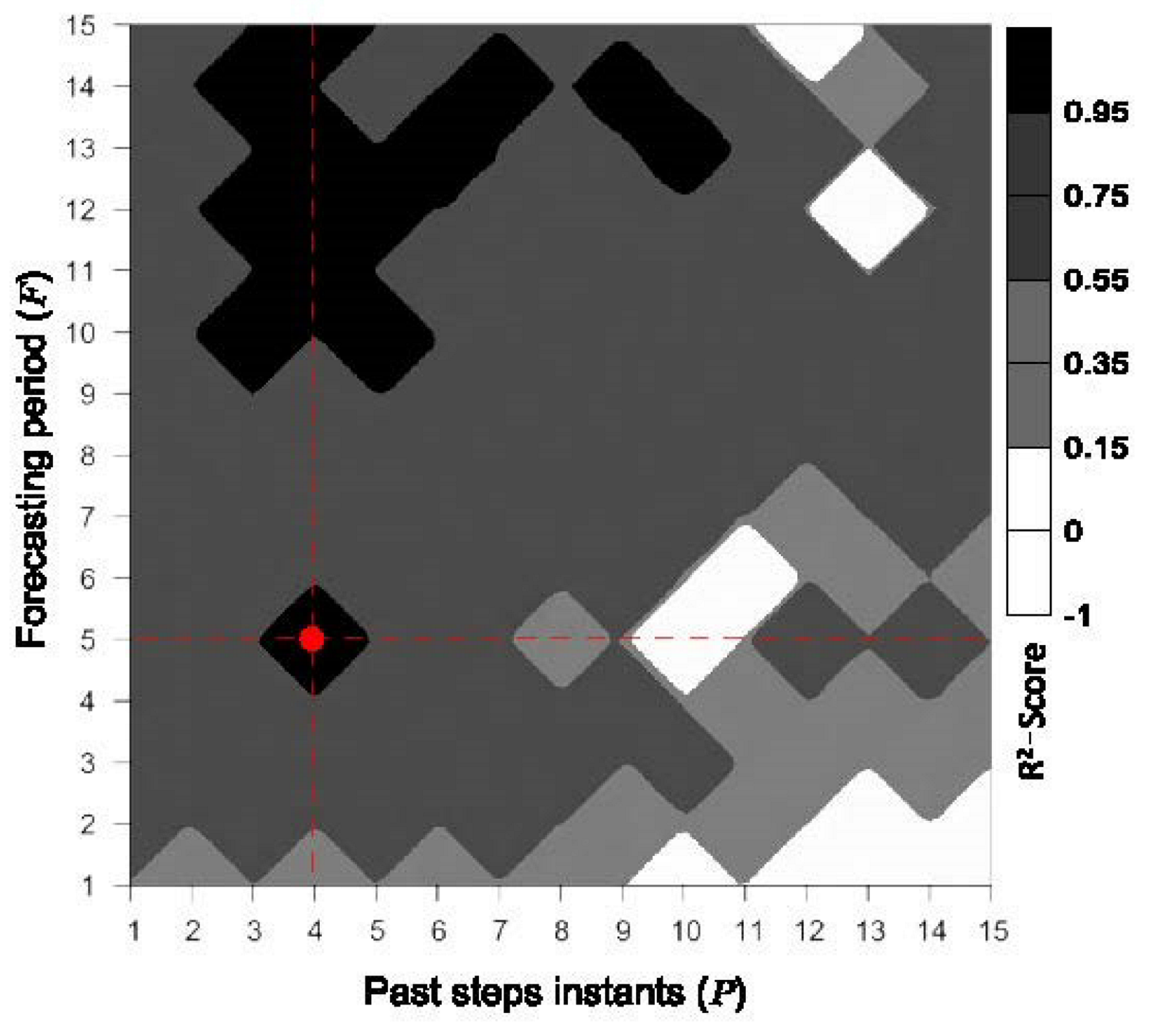
- Past Instants and Forecasting Period: The parameters of past step instants (the number of past instants required to generate the attribute vectors) and the forecasting period (the number of future instants that comprise the prediction interval) are related to the performance and computational cost of the proposed approach. Suitable values for these parameters were analyzed after considering a battery of tests from distinct study areas (Section 3.1 and Section 3.2). Figure 4 depicts a median profile, in terms of the -Score, regarding the estimated algae occurrence concentration. The results indicated that four past step instants and a forecasting period of five instants produced the best outcomes.
- Spatial Context Size: This parameter defines the dimension of the convolution filter applied on the classifications , to measure the occurrence of algae. After performing a series of tests where w varied in 3, 5 and 7, the adoption of provided the best consistency.
- Data Projection: With the aim of alleviating the computational cost, the principal component analysis (PCA) [61] technique was applied to the full set of attribute vectors (i.e., considering all instants and positions), thus allowing the projection of the data onto a feature space of reduced dimensions without losing significant accuracy in the results. More specifically, after a preliminary battery of tests regarding all study areas, the proposed methodology achieved the average values of 0.97, 0.96 and 0.96 for R2-Scores when data projections were applied with 99%, 95% and 90% of explained variance, respectively. However, the computational time drastically decreased by about 70% and 50% when comparing the multidimensional projection with 90% against 99% and 95%, respectively. Consequently, we found that the choice of 90% provided a good trade-off between satisfactory performance and computational cost.

3. Results
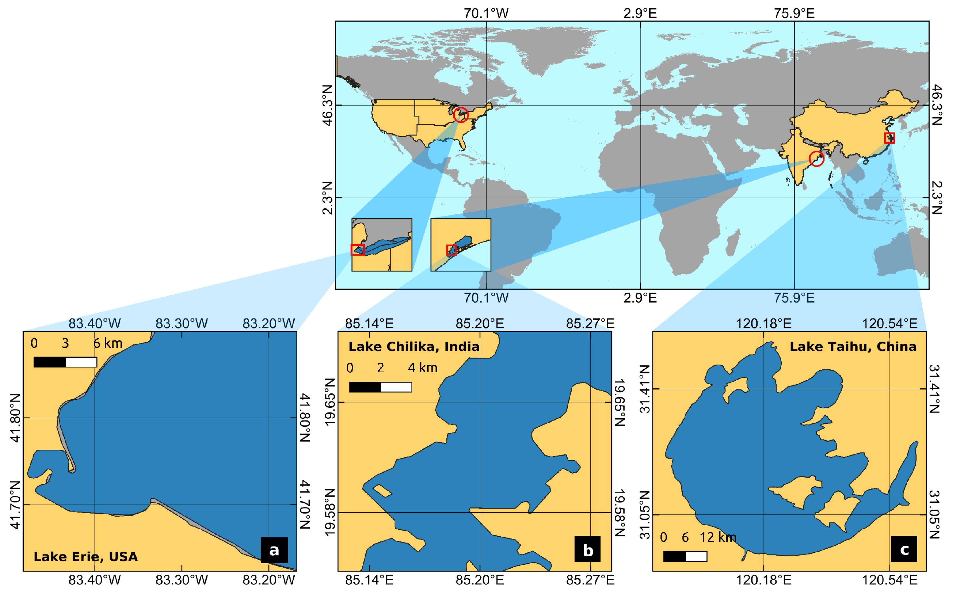
3.1. Study Areas
3.2. Reference Data
3.3. Experimental Analysis
3.4. Discussion
4. Conclusions
Author Contributions
Funding
Data Availability Statement
Conflicts of Interest
References
- Yang, K.; Luo, Y.; Chen, K.; Yang, Y.; Shang, C.; Yu, Z.; Xu, J.; Zhao, Y. Spatial–temporal variations in urbanization in Kunming and their impact on urban lake water quality. Land Degrad. Dev. 2020, 31, 1392–1407. [Google Scholar] [CrossRef]
- Chawla, I.; Karthikeyan, L.; Mishra, A.K. A review of remote sensing applications for water security: Quantity, quality, and extremes. J. Hydrol. 2020, 585, 124826. [Google Scholar]
- Mishra, A.K.; Coulibaly, P. Developments in hydrometric network design: A review. Rev. Geophys. 2009, 47, 1–24. [Google Scholar]
- Wells, M.L.; Trainer, V.L.; Smayda, T.J.; Karlson, B.S.; Trick, C.G.; Kudela, R.M.; Ishikawa, A.; Bernard, S.; Wulff, A.; Anderson, D.M.; et al. Harmful algal blooms and climate change: Learning from the past and present to forecast the future. Harmful Algae 2015, 49, 68–93. [Google Scholar]
- Shi, K.; Zhang, Y.; Qin, B.; Zhou, B. Remote sensing of cyanobacterial blooms in inland waters: Present knowledge and future challenges. Sci. Bull. 2019, 64, 1540–1556. [Google Scholar]
- Gons, H.J. Optical Teledetection of Chlorophyll a in Turbid Inland Waters. Environ. Sci. Technol. 1999, 33, 1127–1132. [Google Scholar]
- Rousso, B.Z.; Bertone, E.; Stewart, R.; Hamilton, D.P. A systematic literature review of forecasting and predictive models for cyanobacteria blooms in freshwater lakes. Water Res. 2020, 182, 115959. [Google Scholar]
- Qi, L.; Hu, C.; Duan, H.; Barnes, B.B.; Ma, R. An EOF-Based Algorithm to Estimate Chlorophyll a Concentrations in Taihu Lake from MODIS Land-Band Measurements: Implications for Near Real-Time Applications and Forecasting Models. Remote Sens. 2014, 6, 10694–10715. [Google Scholar]
- Allen, J.I.; Smyth, T.J.; Siddorn, J.R.; Holt, M. How well can we forecast high biomass algal bloom events in a eutrophic coastal sea? Harmful Algae 2008, 8, 70–76. [Google Scholar]
- Hu, C. A novel ocean color index to detect floating algae in the global oceans. Remote Sens. Environ. 2009, 113, 2118–2129. [Google Scholar]
- Mishra, S.; Mishra, D.R. Normalized Difference Chlorophyll Index: A novel model for remote estimation of chlorophyll-a concentration in turbid productive waters. Remote Sens. Environ. 2012, 117, 394–406. [Google Scholar]
- Zhang, Y.; Ma, R.; Duan, H.; Loiselle, S.A.; Xu, J.; Ma, M. A novel algorithm to estimate algal bloom coverage to subpixel resolution in Lake Taihu. IEEE J. Sel. Top. Appl. Earth Obs. Remote Sens. 2014, 7, 3060–3068. [Google Scholar]
- Houborg, R.; McCabe, M.F.; Angel, Y.; Middleton, E.M. Detection of chlorophyll and leaf area index dynamics from sub-weekly hyperspectral imagery. In Proceedings of the Remote Sensing for Agriculture, Ecosystems, and Hydrology XVIII, International Society for Optics and Photonics, Edinburgh, UK, 26–29 September 2016; Volume 9998, p. 999812. [Google Scholar]
- Watanabe, F.; Alcantara, E.; Rodrigues, T.; Rotta, L.; Bernardo, N.; Imai, N. Remote sensing of the chlorophyll-a based on OLI/Landsat-8 and MSI/Sentinel-2A (Barra Bonita reservoir, Brazil). An. Acad. Bras. Ciências 2018, 90, 1987–2000. [Google Scholar]
- Yuan, Q.; Shen, H.; Li, T.; Li, Z.; Li, S.; Jiang, Y.; Xu, H.; Tan, W.; Yang, Q.; Wang, J.; et al. Deep learning in environmental remote sensing: Achievements and challenges. Remote Sens. Environ. 2020, 241, 111716. [Google Scholar]
- Martínez-Álvarez, F.; Tien Bui, D. Advanced Machine Learning and Big Data Analytics in Remote Sensing for Natural Hazards Management. Remote Sens. 2020, 12, 301. [Google Scholar]
- Zhang, T.; Huang, M.; Wang, Z. Estimation of chlorophyll-a Concentration of lakes based on SVM algorithm and Landsat 8 OLI images. Environ. Sci. Pollut. Res. 2020, 27, 14977–14990. [Google Scholar]
- Ananias, P.H.M.; Negri, R.G. Anomalous behaviour detection using one-class support vector machine and remote sensing images: A case study of algal bloom occurrence in inland waters. Int. J. Digit. Earth 2021, 14, 921–942. [Google Scholar]
- Silveira Kupssinskü, L.; Thomassim Guimarães, T.; Menezes de Souza, E.; Zanotta, C.D.; Roberto Veronez, M.; Gonzaga, L.; Mauad, F.F. A Method for Chlorophyll-a and Suspended Solids Prediction through Remote Sensing and Machine Learning. Sensors 2020, 20, 2125. [Google Scholar]
- Cho, H.; Choi, U.; Park, H. Deep learning application to time-series prediction of daily chlorophyll-a concentration. WIT Trans. Ecol. Environ. 2018, 215, 157–163. [Google Scholar]
- Lee, M.S.; Park, K.A.; Chae, J.; Park, J.E.; Lee, J.S.; Lee, J.H. Red tide detection using deep learning and high-spatial resolution optical satellite imagery. Int. J. Remote Sens. 2020, 41, 5838–5860. [Google Scholar]
- Barzegar, R.; Aalami, M.T.; Adamowski, J. Short-term water quality variable prediction using a hybrid CNN–LSTM deep learning model. Stoch. Environ. Res. Risk Assess. 2020, 34, 415–433. [Google Scholar]
- Yu, Z.; Yang, K.; Luo, Y.; Shang, C. Spatial-temporal process simulation and prediction of chlorophyll-a concentration in Dianchi Lake based on wavelet analysis and long-short term memory network. J. Hydrol. 2020, 582, 124488. [Google Scholar] [CrossRef]
- Körting, T.S.; Fonseca, L.M.G.; Castejon, E.F.; Namikawa, L.M. Improvements in Sample Selection Methods for Image Classification. Remote Sens. 2014, 6, 7580–7591. [Google Scholar]
- Wang, X.; Yan, H.; Huo, C.; Yu, J.; Pant, C. Enhancing Pix2Pix for Remote Sensing Image Classification. In Proceedings of the 2018 24th International Conference on Pattern Recognition (ICPR), Beijing, China, 20–24 August 2018; pp. 2332–2336. [Google Scholar]
- Cortes, C.; Vapnik, V. Support-vector networks. Mach. Learn. 1995, 20, 273–297. [Google Scholar]
- Breiman, L. Random forests. Mach. Learn. 2001, 45, 5–32. [Google Scholar]
- Vapnik, V. Estimation of Dependences Based on Empirical Data; Springer: Berlin/Heidelberg, Germany, 1982. [Google Scholar] [CrossRef]
- Mountrakis, G.; Im, J.; Ogole, C. Support Vector Machines in Remote Sensing: A review. ISPRS J. Photogramm. Remote Sens. Soc. 2011, 66, 247–259. [Google Scholar]
- Shawe-Taylor, J.; Cristianini, N. Kernel Methods for Pattern Analysis; Cambridge University Press: Cambridge, UK, 2004. [Google Scholar]
- Bruzzone, L.; Persello, C. A Novel Context-Sensitive Semisupervised SVM Classifier Robust to Mislabeled Training Samples. IEEE Trans. Geosci. Remote Sens. 2009, 47, 2142–2154. [Google Scholar]
- Theodoridis, S.; Koutroumbas, K. Pattern Recognition, 4th ed.; Academic Press: San Diego, CA, USA, 2008; p. 984. [Google Scholar]
- Dietterich, T.G. Ensemble learning. In The Handbook of Brain Theory and Neural Networks; MIT Press: Cambridge, MA, USA, 2002; Volume 2, pp. 110–125. [Google Scholar]
- Hochreiter, S.; Schmidhuber, J. Long Short-Term Memory. Neural Comput. 1997, 9, 1735–1780. [Google Scholar] [CrossRef]
- McFeeeters, S.K. The use of the Normalized Difference Water Index (NDWI) in the delineation of open water features. Int. J. Remote Sens. 1996, 17, 1425–1432. [Google Scholar]
- Gao, B.C. NDWI—A normalized difference water index for remote sensing of vegetation liquid water from space. Remote Sens. Environ. 1996, 58, 257–266. [Google Scholar]
- Xu, H. Modification of normalised difference water index (NDWI) to enhance open water features in remotely sensed imagery. Int. J. Remote Sens. 2006, 27, 3025–3033. [Google Scholar]
- Rouse, J.W., Jr.; Haas, R.H.; Schell, J.; Deering, D. Monitoring the Vernal Advancement and Retrogradation (Green Wave Effect) of Natural Vegetation; Texas A&M University: College Station, TX, USA, 1973. [Google Scholar]
- Huete, A. A soil-adjusted vegetation index (SAVI). Remote Sens. Environ. 1988, 25, 295–309. [Google Scholar]
- Liu, H.Q.; Huete, A. A feedback based modification of the NDVI to minimize canopy background and atmospheric noise. IEEE Trans. Geosci. Remote Sens. 1995, 33, 457–465. [Google Scholar]
- Wang, Z.; Liu, C.; Huete, A. From AVHRR-NDVI to MODIS-EVI: Advances in vegetation index research. Acta Ecol. Sin. 2003, 23, 979–987. [Google Scholar]
- Zhao, D. Application of NDVI to detecting algal bloom in the Bohai Sea of China from AVHRR. In Ocean Remote Sensing and Applications, Proceedings of the Third International Asia-Pacific Environmental Remote Sensing Remote Sensing of the Atmosphere, Ocean, Environment, and Space, Hangzhou, China, 24–26 October 2002; SPIE: Bellingham, WA, USA, 2003; Volume 4892, pp. 241–246. [Google Scholar]
- Han-Qiu, X. A study on information extraction of water body with the modified normalized difference water index (MNDWI). J. Remote Sens. 2005, 5, 589–595. [Google Scholar]
- Alawadi, F. Detection of surface algal blooms using the newly developed algorithm surface algal bloom index (SABI). In Remote Sensing of the Ocean, Sea Ice, and Large Water Regions 2010, Proceedings of the SPIE Remote Sensing, Toulouse, France, 20 September 2010; SPIE: Bellingham, WA, USA, 2010; Volume 7825, pp. 45–58. [Google Scholar]
- Oyama, Y.; Fukushima, T.; Matsushita, B.; Matsuzaki, H.; Kamiya, K.; Kobinata, H. Monitoring levels of cyanobacterial blooms using the visual cyanobacteria index (VCI) and floating algae index (FAI). Int. J. Appl. Earth Obs. Geoinf. 2015, 38, 335–348. [Google Scholar]
- Rodell, M.; Houser, P.R.; Jambor, U.; Gottschalck, J.; Mitchell, K.; Meng, C.J.; Arsenault, K.; Cosgrove, B.; Radakovich, J.; Bosilovich, M.; et al. The Global Land Data Assimilation System. Bull. Am. Meteorol. Soc. 2004, 85, 381–394. [Google Scholar]
- Lehner, B.; Verdin, K.; Jarvis, A. New Global Hydrography Derived From Spaceborne Elevation Data. Eos Trans. Am. Geophys. Union 2008, 89, 93–94. [Google Scholar]
- Takaku, J.; Tadono, T.; Doutsu, M.; Ohgushi, F.; Kai, H. Updates OF ‘AW3D30’ Alos Global Digital Surface Model with Other Open Access Datasets. Int. Arch. Photogramm. Remote Sens. Spat. Inf. Sci. 2020, 43, 183–189. [Google Scholar]
- Wan, Z.; Hook, S.; Hulley, G. MOD11A1 MODIS/Terra Land Surface Temperature/Emissivity Daily L3 Global 1km SIN Grid V006; Type: Dataset; NASA EOSDIS Land Processes DAAC: Sioux Falls, SD, USA, 2015.
- McKinney, W. Python for Data Analysis: Data Wrangling with PANDAS, NumPy, and IPython; O’Reilly Media, Inc.: Sebastopol, CA, USA, 2012. [Google Scholar]
- van Rossum, G.; Drake, F.L. The Python Language Reference Manual; Network Theory Ltd.: Godalming, UK, 2011. [Google Scholar]
- van der Walt, S.; Colbert, S.C.; Varoquaux, G. The NumPy Array: A Structure for Efficient Numerical Computation. Comput. Sci. Eng. 2011, 13, 22–30. [Google Scholar]
- McKinney, W. Data structures for statistical computing in Python. In Proceedings of the 9th Python in Science Conference, Austin, TX, USA, 28 June–3 July 2010; Volume 445, pp. 51–56. [Google Scholar]
- Pedregosa, F.; Varoquaux, G.; Gramfort, A.; Michel, V.; Thirion, B.; Grisel, O.; Blondel, M.; Prettenhofer, P.; Weiss, R.; Dubourg, V.; et al. Scikit-learn: Machine learning in Python. J. Mach. Learn. Res. 2011, 12, 2825–2830. [Google Scholar]
- Ketkar, N. Introduction to keras. In Deep learning with Python; Springer: Berlin/Heidelberg, Germany, 2017; pp. 97–111. [Google Scholar]
- GEE-API. Google Earth Engine API. 2019. Available online: https://developers.google.com/earth-engine (accessed on 24 July 2022).
- USGS. MODIS/Terra Surface Reflectance Daily L2G Global 1 km and 500 m. 2020. Available online: https://lpdaac.usgs.gov/products/mod09gav006/ (accessed on 24 July 2022).
- Rastrigin, L. The convergence of the random search method in the extremal control of a many parameter system. Autom. Remote Control. 1963, 24, 1337–1342. [Google Scholar]
- Baba, N. Convergence of a random optimization method for constrained optimization problems. J. Optim. Theory Appl. 1981, 33, 451–461. [Google Scholar]
- Bergstra, J.; Bengio, Y. Random search for hyper-parameter optimization. J. Mach. Learn. Res. 2012, 13, 281–305. [Google Scholar]
- Jolliffe, I. Principal component analysis. Encycl. Stat. Behav. Sci. 2005. [Google Scholar] [CrossRef]
- Congalton, R.G.; Green, K. Assessing the Accuracy of Remotely Sensed Data; CRC Press: Boca Raton, FL, USA, 2009; p. 183. [Google Scholar]
- van Rijsbergen, C.J. Information Retrieval, 2nd ed.; Butterworths: London, UK, 1979. [Google Scholar]
- Draper, N.R.; Smith, H. Applied Regression Analysis; John Wiley & Sons: Hoboken, NJ, USA, 1998; Volume 326. [Google Scholar]
- Chai, T.; Draxler, R.R. Root mean square error (RMSE) or mean absolute error (MAE)? – Arguments against avoiding RMSE in the literature. Geosci. Model Dev. 2014, 7, 1247–1250. [Google Scholar] [CrossRef]
- Bolsenga, S.J.; Herdendorf, C.E. Lake Erie and Lake St. Clair Handbook; Wayne State University Press: Detroit, MI, USA, 1993. [Google Scholar]
- Zhu, M.; Zhu, G.; Zhao, L.; Yao, X.; Zhang, Y.; Gao, G.; Qin, B. Influence of algal bloom degradation on nutrient release at the sediment–water interface in Lake Taihu, China. Environ. Sci. Pollut. Res. 2012, 20, 1803–1811. [Google Scholar]
- Stumpf, R.P.; Wynne, T.T.; Baker, D.B.; Fahnenstiel, G.L. Interannual Variability of Cyanobacterial Blooms in Lake Erie. PLoS ONE 2012, 7, e42444. [Google Scholar]
- Sengupta, M.; Anandurai, R.; Nanda, S.; Datti, A.A. Geospatial identification of algal blooms in inland waters: A post cyclone case study of Chilka Lake, Odisha, India. RASAYAN J. Chem. 2017, 10, 234–239. [Google Scholar]
- Panigrahi, J.K. Water Quality, Biodiversity and Livelihood Issues: A Case Study of Chilika Lake, India. In Proceedings of the 2007 Atlanta Conference on Science, Technology and Innovation Policy, Atlanta, GA, USA, 19–20 October 2007; pp. 1–6. [Google Scholar]
- Ranjan, R. A forestry-based PES mechanism for enhancing the sustainability of Chilika Lake through reduced siltation loading. For. Policy Econ. 2019, 106, 101944. [Google Scholar] [CrossRef]
- Liu, L.; Dong, Y.; Kong, M.; Zhou, J.; Zhao, H.; Wang, Y.; Zhang, M.; Wang, Z. Towards the comprehensive water quality control in Lake Taihu: Correlating chlorphyll a and water quality parameters with generalized additive model. Sci. Total Environ. 2020, 705, 135993. [Google Scholar] [CrossRef] [PubMed]
- Gao, Y.; Zhu, G.; Paerl, H.W.; Qin, B.; Yu, J.; Song, Y. A study of bioavailable phosphorus in the inflowing rivers of Lake Taihu, China. Aquat. Sci. 2020, 82, 1. [Google Scholar]
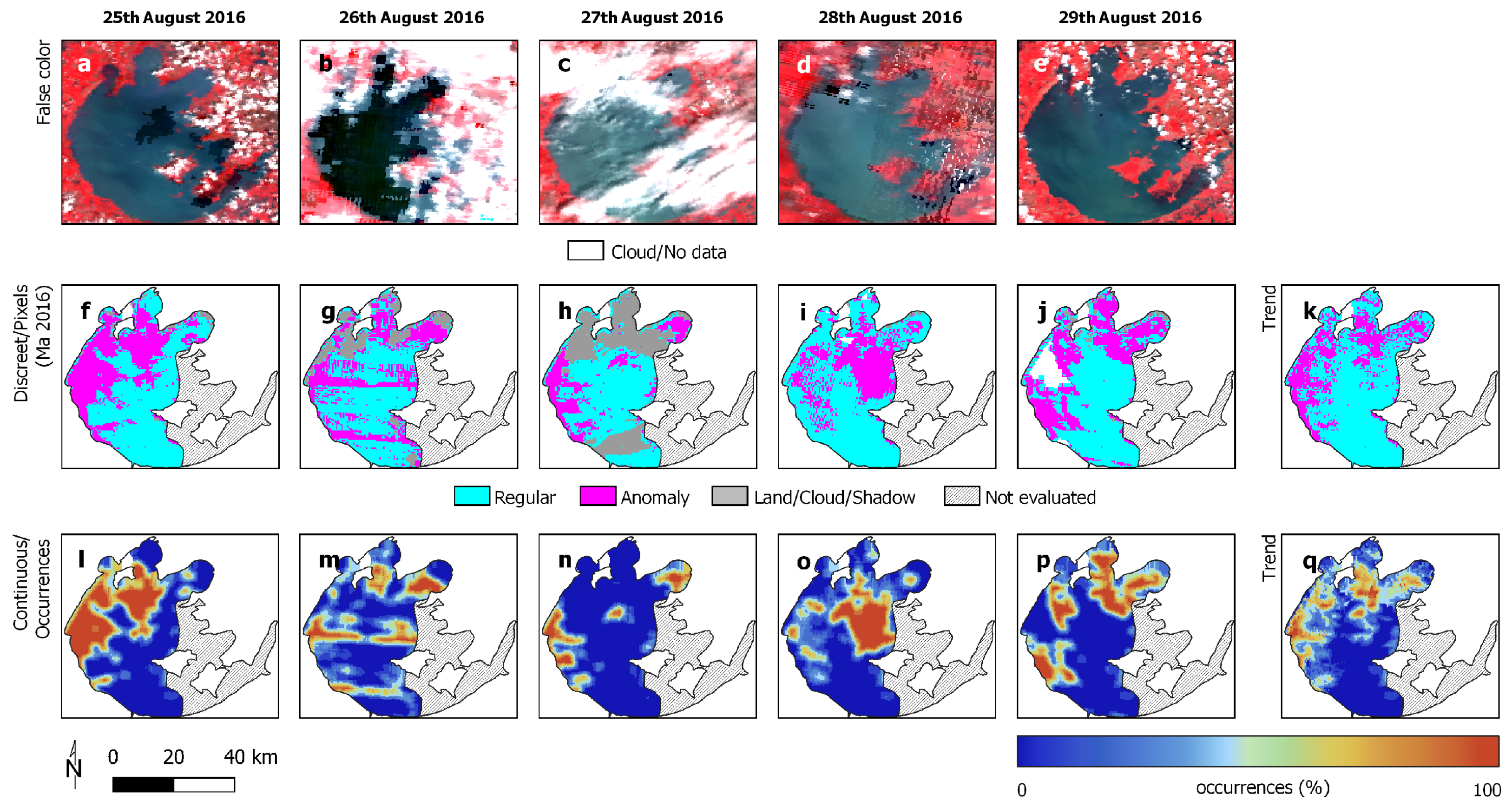
- Ma, R. Lake Taihu Chlorophyll Inversion Product Data Set (2016); National Earth System Science Data Center, National Science and Technology Infrastructure of China: Beijing, China, 2016. [Google Scholar]
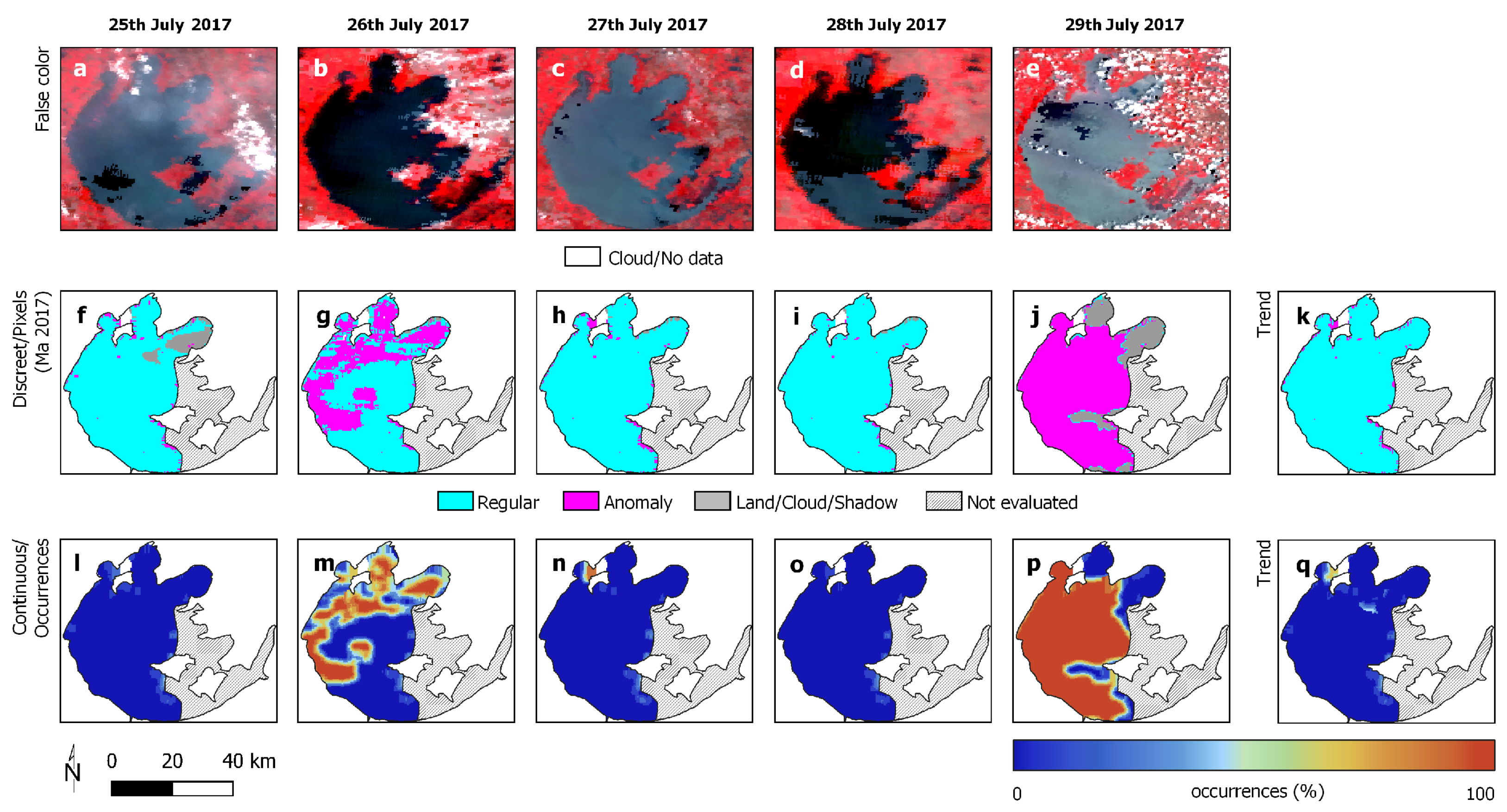
- Ma, R. Lake Taihu Chlorophyll Inversion Product Data Set (2017); National Earth System Science Data Center, National Science and Technology Infrastructure of China: Beijing, China, 2017. [Google Scholar]
- Xu, H.; Paerl, H.W.; Qin, B.; Zhu, G.; Hall, N.S.; Wu, Y. Determining Critical Nutrient Thresholds Needed to Control Harmful Cyanobacterial Blooms in Eutrophic Lake Taihu, China. Environ. Sci. Technol. 2015, 49, 1051–1059. [Google Scholar] [CrossRef] [PubMed]
- Wang, M.; Strokal, M.; Burek, P.; Kroeze, C.; Ma, L.; Janssen, A.B. Excess nutrient loads to Lake Taihu: Opportunities for nutrient reduction. Sci. Total Environ. 2019, 664, 865–873. [Google Scholar] [CrossRef] [PubMed]
- Kane, D.D.; Conroy, J.D.; Richards, R.P.; Baker, D.B.; Culver, D.A. Re-eutrophication of Lake Erie: Correlations between tributary nutrient loads and phytoplankton biomass. J. Great Lakes Res. 2014, 40, 496–501. [Google Scholar] [CrossRef]
- Scavia, D.; Allan, J.D.; Arend, K.K.; Bartell, S.; Beletsky, D.; Bosch, N.S.; Brandt, S.B.; Briland, R.D.; Daloğlu, I.; DePinto, J.V.; et al. Assessing and addressing the re-eutrophication of Lake Erie: Central basin hypoxia. J. Great Lakes Res. 2014, 40, 226–246. [Google Scholar] [CrossRef]
- Barik, S.K.; Bramha, S.N.; Mohanty, A.K.; Bastia, T.K.; Behera, D.; Rath, P. Sequential extraction of different forms of phosphorus in the surface sediments of Chilika Lake. Arab. J. Geosci. 2016, 9, 135. [Google Scholar] [CrossRef]


| Spectral Index | Expression | Algae Threshold | Reference |
|---|---|---|---|
| NDVI | >−0.15 | [42] | |
| MNDWI | <0 | [37] | |
| SABI | >−0.1 | [44] | |
| FAI | >−0.004 | [45] |
| Lake Erie | ||
|---|---|---|
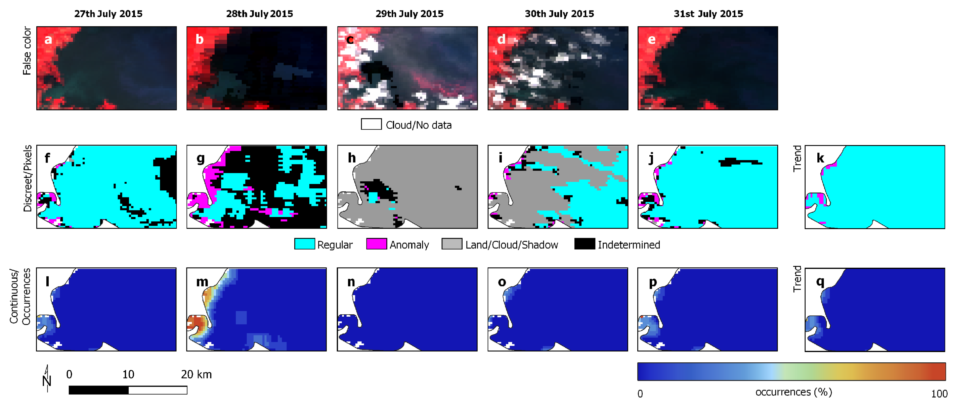
| 11–15 October 2013 | 27–31 July 2015 | |
| Regular | 277,328 | 233,137 |
| Anomaly | 19,041 | 13,210 |
| Average occurrence | 0.8% | 3.2% |
| Stand. deviation occurrences | 4.5% | 11.3% |
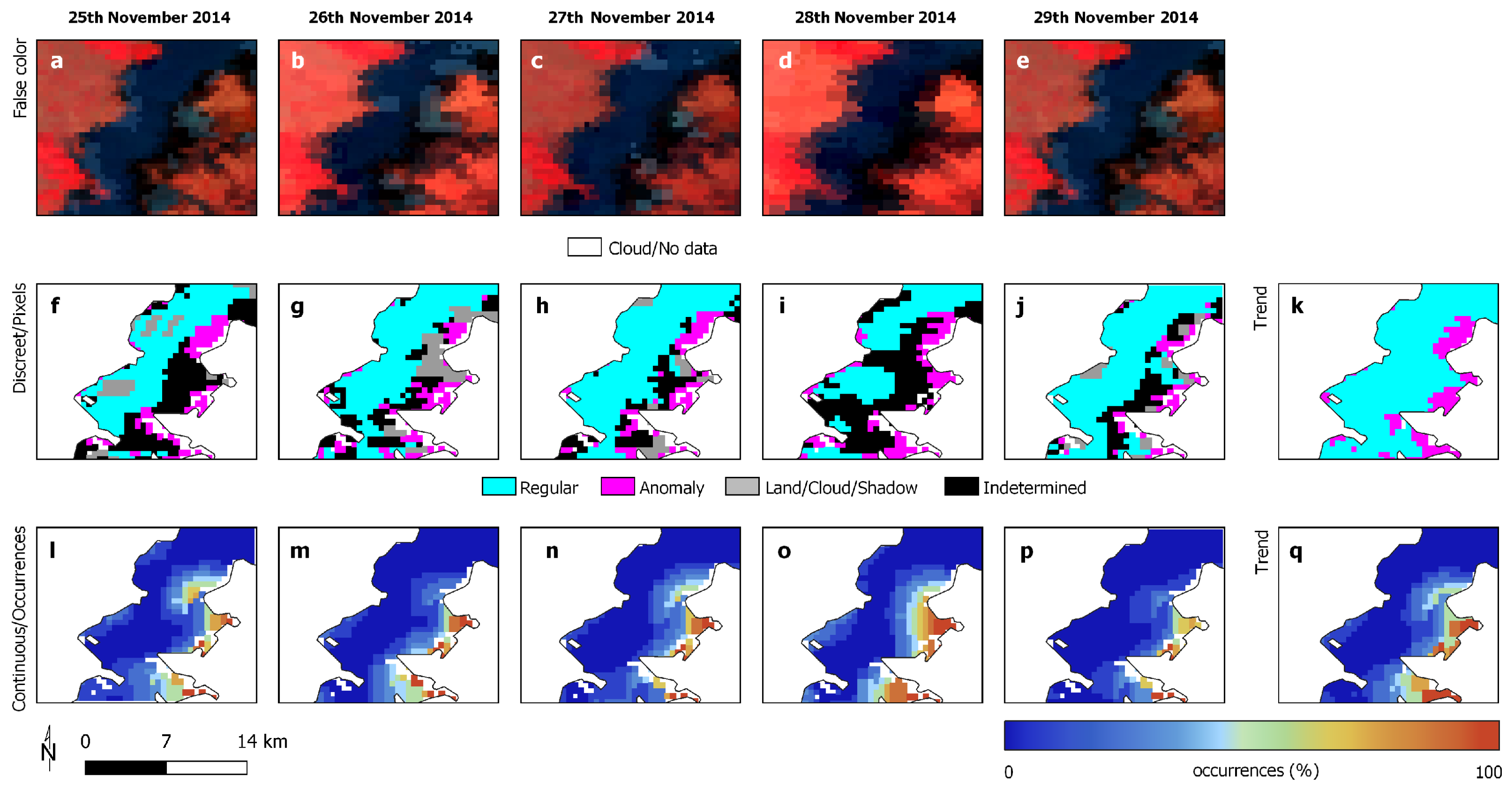
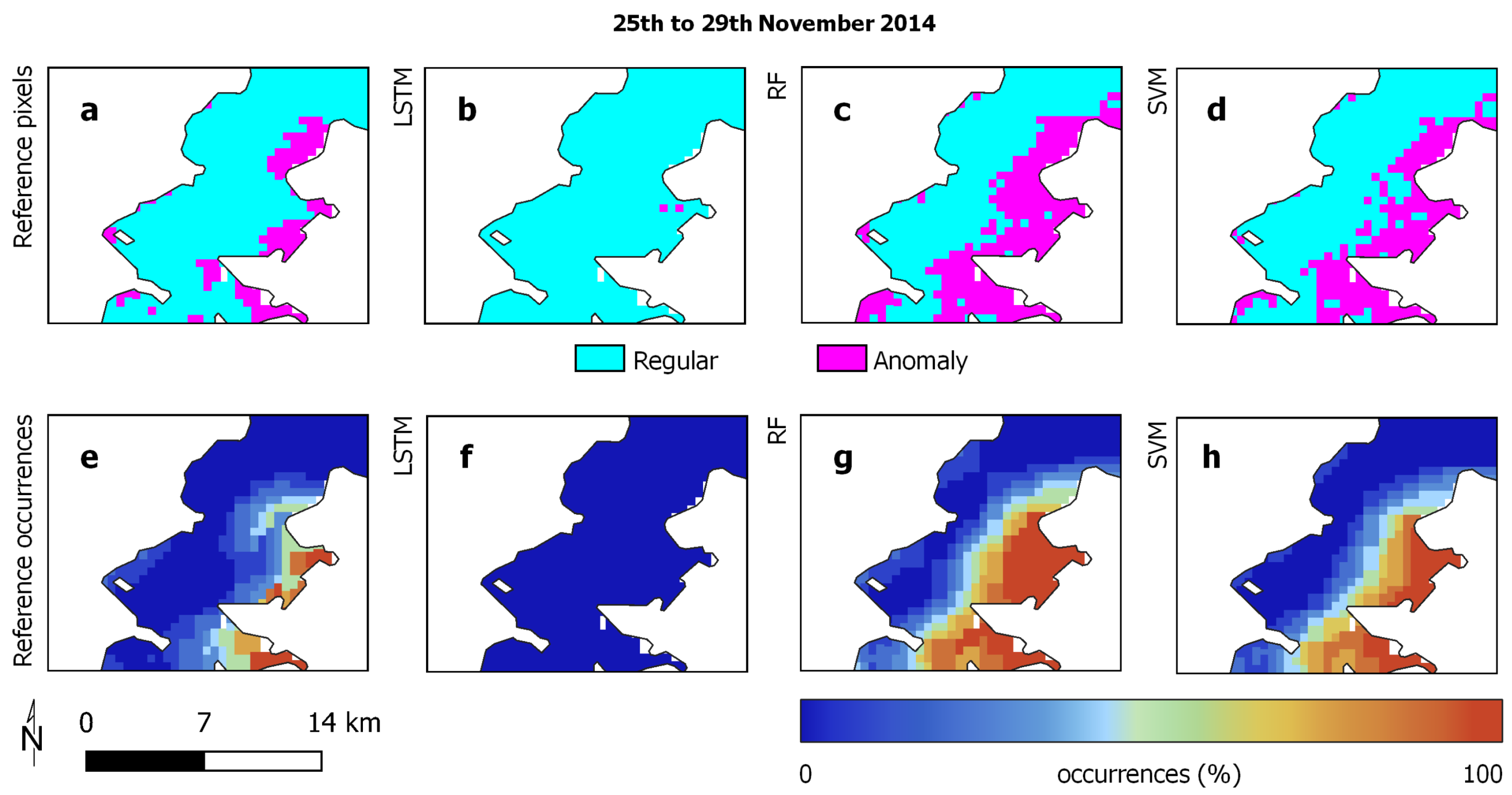
| Lake Chilika | ||
| 25–29 November 2014 | ||
| Regular | 41,272 | |
| Anomaly | 21,692 | |
| Average occurrence | 19.4% | |
| Stand. deviation occurrences | 26.5% | |
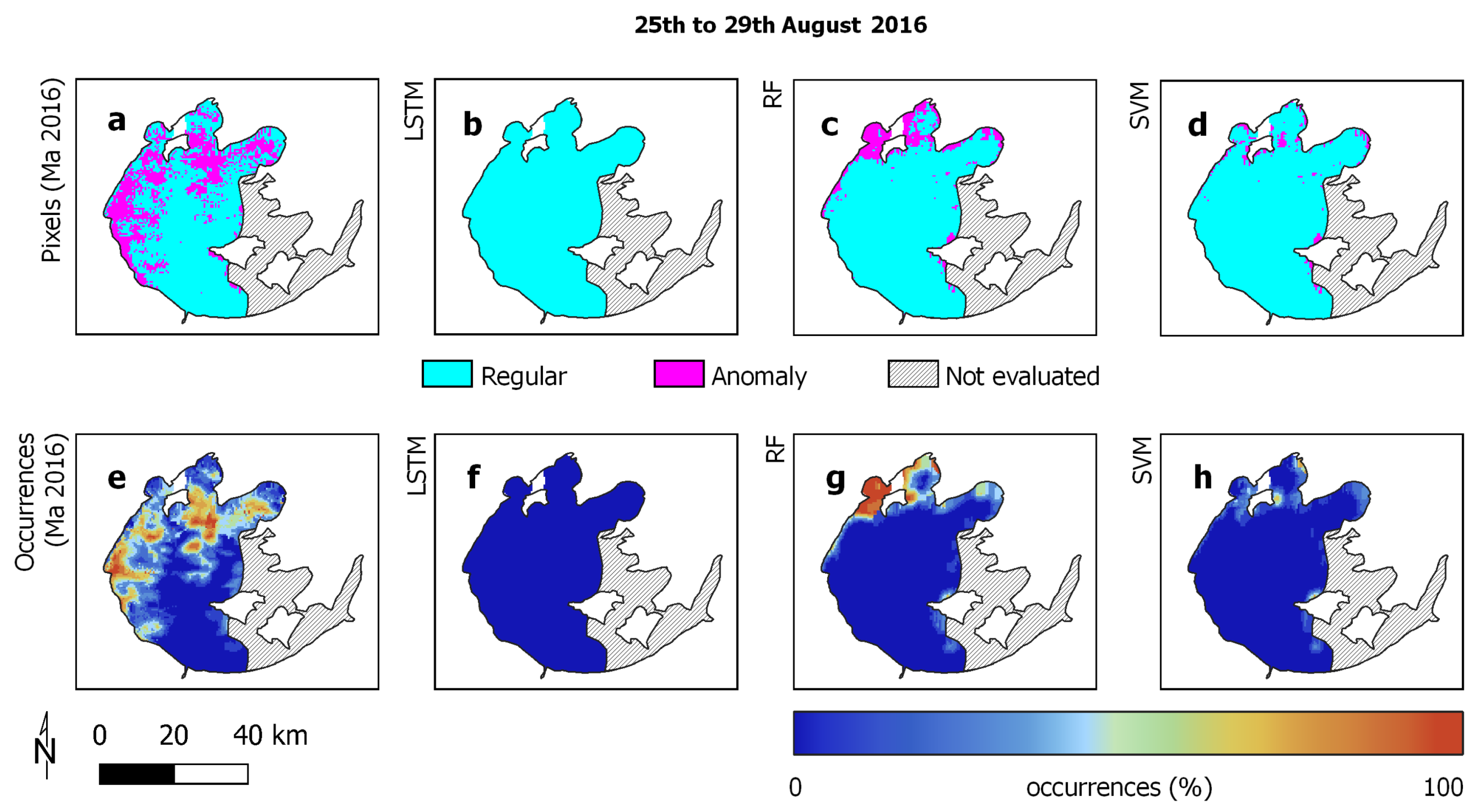
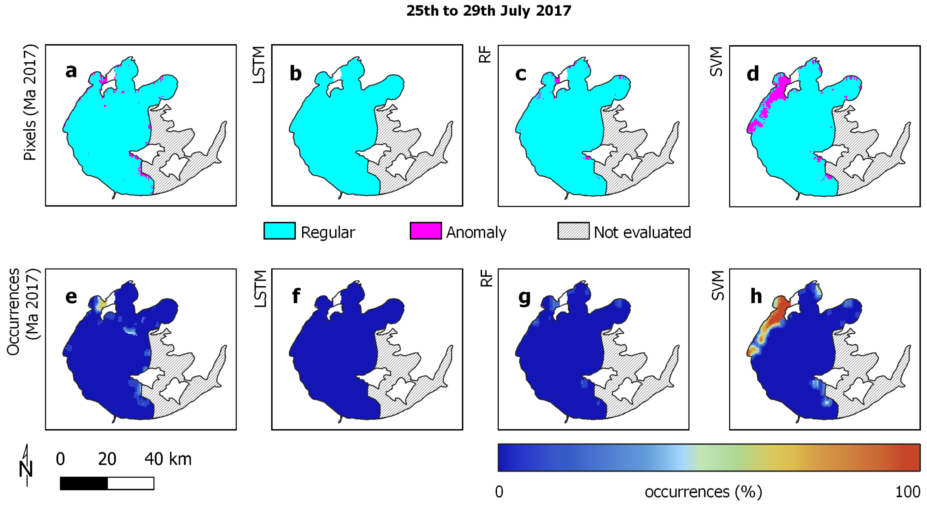
| Lake Taihu | ||
| 25–29 August 2016 | 25–29 July 2017 | |
| Regular | 631,398 | 1,259,410 |
| Anomaly | 72,399 | 142,685 |
| Average occurrence | 22.6% | 19.1% |
| Stand. deviation occ. | 27.7% | 33.8% |
Publisher’s Note: MDPI stays neutral with regard to jurisdictional claims in published maps and institutional affiliations. |
© 2022 by the authors. Licensee MDPI, Basel, Switzerland. This article is an open access article distributed under the terms and conditions of the Creative Commons Attribution (CC BY) license (https://creativecommons.org/licenses/by/4.0/).
Share and Cite
Ananias, P.H.M.; Negri, R.G.; Dias, M.A.; Silva, E.A.; Casaca, W. A Fully Unsupervised Machine Learning Framework for Algal Bloom Forecasting in Inland Waters Using MODIS Time Series and Climatic Products. Remote Sens. 2022, 14, 4283. https://doi.org/10.3390/rs14174283
Ananias PHM, Negri RG, Dias MA, Silva EA, Casaca W. A Fully Unsupervised Machine Learning Framework for Algal Bloom Forecasting in Inland Waters Using MODIS Time Series and Climatic Products. Remote Sensing. 2022; 14(17):4283. https://doi.org/10.3390/rs14174283
Chicago/Turabian StyleAnanias, Pedro Henrique M., Rogério G. Negri, Maurício A. Dias, Erivaldo A. Silva, and Wallace Casaca. 2022. "A Fully Unsupervised Machine Learning Framework for Algal Bloom Forecasting in Inland Waters Using MODIS Time Series and Climatic Products" Remote Sensing 14, no. 17: 4283. https://doi.org/10.3390/rs14174283
APA StyleAnanias, P. H. M., Negri, R. G., Dias, M. A., Silva, E. A., & Casaca, W. (2022). A Fully Unsupervised Machine Learning Framework for Algal Bloom Forecasting in Inland Waters Using MODIS Time Series and Climatic Products. Remote Sensing, 14(17), 4283. https://doi.org/10.3390/rs14174283