Validating Ionospheric Scintillation Indices Extracted from 30s-Sampling-Interval GNSS Geodetic Receivers with Long-Term Ground and In-Situ Observations in High-Latitude Regions

Abstract

As a frequently-occurred phenomenon in the high-latitude region, ionospheric scintillations affect the stable service of the positioning navigation and timing service of the Global Navigation Satellite System (GNSS), calling for an urgent need of monitoring the scintillations accurately. The monitoring of scintillations usually adopts a special type of receiver, called an ionospheric scintillation monitoring receiver (ISMR), which cannot cover the whole high-latitude region due to its loss distribution. Geodetic receivers are densely distributed, but set at a 30s-sampling-interval usually. It is a controversial issue, namely, the accuracy of the scintillation index extracted from 30s-sampling-interval observations. This paper evaluates the accuracy of two 30s-sampling-interval indices in monitoring scintillations from both the time and space aspects using observations collected in the whole year of 2020. The accuracy in the time aspect is assessed with the phase scintillation index from ISMR as the reference through the following three-pronged approaches, i.e., the accuracy of the daily scintillation occurrence rates in the year 2020, the correlation with space weather parameters, and the variation pattern of the scintillation occurrence rate with the local time and day of the year 2020. The accuracy in space is studied based on the scintillation grid model considering the following two aspects, i.e., the scintillation monitoring performance in a Swarm satellite observation arc, and the statistical scintillation occurrence rate in the whole research region throughout the year 2020. The results of this paper reveal the efficiency of the 30s-sampling-interval scintillation indices in monitoring scintillations and detecting the occurrence patterns in the high-latitude region. The outcome of this paper can provide a basic idea for introducing the widely distributed geodetic receivers to monitor and model the scintillations in the high-latitude region.

1. Introduction

Electromagnetic waves passing through ionospheric irregularities can have rapid fluctuations in both the amplitude and phase, which is usually known as an ionospheric scintillation [1]. The signal tracking and acquisition process of Global Navigation Satellite System (GNSS) receivers can be highly affected by severe scintillations, leading to cycle slips or even a loss of loop. To maintain the stable service of the GNSS, there is in an urgent need for monitoring scintillations effectively.

The ionospheric scintillation monitoring receiver (ISMR) is the typical equipment that is widely used in monitoring scintillations. An ISMR collects data at a 50 Hz rate, making a substantial memory necessary to store the large amount of data. A highly stable receiver clock is also required to maintain the tracking performance during scintillations. Due to the large memory and the stable clock, the price of an ISMR is usually high, which limits the distribution of ISMRs, especially in the high-latitude region. To the knowledge of the authors, only about 30 ISMR stations are located in the high-latitude region [2,3,4]; thus, the sparse distribution of ISMR stations makes it impossible to study the scintillations in a large area.

Compared to ISMRs, geodetic receivers are less expensive and more densely distributed [5]. The observations of geodetic GNSS receivers can be freely available at several agencies, e.g., the International GNSS service (IGS), the National Oceanic and Atmospheric Administration (NOAA), Canadian Geodetic Survey (CGS), and the United States Satellite Navigation System and Crust Deformation Observation and Research University Alliance. During the past several years, a number of studies have been conducted to try to introduce these dense geodetic GNSS stations to assist the monitoring of ionospheric scintillations, especially from the aspect of developing a suitable scintillation index based on the observations of geodetic receivers [6,7,8,9,10,11]. Most of the existing scintillation indices, which are suitable for the geodetic receivers, were proposed based on 1s-sampling-interval observations, without considering the fact that most of the standard geodetic receivers are set to collecting observations at 30s-sampling-interval. It will be more practical and meaningful to introduce these 30s-sampling-interval observations into the study of scintillations, so as to achieve the aim of monitoring scintillations in a large region; however, the changes in the sampling interval affect the accuracy of the above geodetic-receiver-based scintillation indices significantly [12], making it still a controversial issue of whether the scintillation index extracted from 30s-sampling-interval GNSS observations are reliable to be used in monitoring scintillations.

The accuracy of the scintillation indices extracted from geodetic receivers are traditionally verified in the time series with the scintillation indices provided by ISMRs as the references, as it is impossible to achieve space-continuous large-area scintillation monitoring results using an ISMR, especially in the high-latitude region. With the increased number of launched low Earth polar orbiting satellites, it is possible to research the ionospheric scintillations in a large region. Early studies mainly adopted the in situ ion density and electric field data of the Dynamics Explorer (DE) 2 satellites to study the ionospheric irregularities in the high-latitude region with the power spectral analysis method [13,14]. During the past a few years, Swarm satellites have been widely used in studying the ionospheric irregularities, such as the high-latitude polar cap patches [15,16,17,18,19], using their in situ plasma density measurements. These studies provide the initial feasibility research on the cross-comparison between the ground and the in situ ionospheric observations.

Pi et al. [20] proposed the rate of total electron content (TEC) index (ROTI), which can be applied in 30s-sampling-interval data by increasing the period for taking the standard deviation to 5 min. Zhao et al. [21] proposed a scintillation index extracted from each carrier of GNSS observations with the continuous wavelet transform technique. Although this index was initially proposed to be applied in the 1s-sampling-interval, it has been tested to achieve a good scintillation monitoring performance with 30s-sampling-interval observations in the research group of the authors. Taking these two scintillation indices as the examples, this paper aims to validate the accuracy of the scintillation indices extracted from 30s-sampling-interval observations in monitoring scintillations in the high-latitude region. The verification will be conducted from both the time and space aspects with the phase scintillation index of the ISMR and the in situ observations of Swarm satellites as the references.

2. Methods to Estimating the Scintillation Indices

In order to analyze the scintillation monitoring performance of the two scintillation indices, i.e., ROTI and the ${\sigma }_{\varnothing f,30s}$ index extracted from 30s-sampling-interval observations [21], the phase scintillation index from the ISMR and the RODI from the in situ Swarm observations were selected as the references. This section will briefly introduce the calculation of these indices.

2.1. Phase Scintillation Index (${\sigma }_{\varphi }$) from 50 Hz ISMR Observations

The ${\sigma }_{\varphi }$ index was extracted from the 50 Hz ISMR carrier phase observations. Compared to the amplitude scintillation index, the ${\sigma }_{\varphi }$ index is believed to be more suitable for monitoring scintillations in the high-latitude region [22,23]. The ${\sigma }_{\varphi }$ index can be estimated as follows:

$${\sigma }_{\varphi }=\sqrt{{\varphi }^2-{\varphi }^2}$$

(1)

where $\varphi$ represents the carrier phase measurement detrended by the six-order Butterworth filter with 0.1 Hz as the cutoff frequency. The optimal cutoff frequency for the high-latitude region is still a controversial problem. Although some of the existing research showed that the 0.1 Hz cutoff frequency may lead to the overestimation of the scintillation index, and suggested a higher cutoff frequency [24,25], it should be noted that no agreement has been reached on the optimal cutoff frequency. Our previous research revealed that the increased cutoff frequency could lead to a decrease in the duration and magnitude of the detected scintillation, while a high correlation was obtained between the scintillation index extracted with the 0.1 Hz cutoff frequency and that with a higher frequency [23], indicating that an equivalent scintillation monitoring performance can be expected between the scintillations with different cutoff frequencies by changing the threshold of determining the occurrence of the scintillation. Therefore, we think it is still reasonable to adopt the ${\sigma }_{\varphi }$ index estimated with a 0.1 Hz cutoff frequency to evaluate the performance of the scintillation indices from 30s-sampling-interval observations. Additionally, 60 s was adopted as the moving window for calculating the ${\sigma }_{\varphi }$ index, while a 0.2 rad was selected as the threshold.

2.2. Rate of Change of Density Index (RODI) Estimated from the Electric Field Instrument of Swarm Satellites

Swarm measures the in situ electron density ($N_e$) with its electric field instrument, namely, the Langmuir probe, at a 2 Hz sampling rate. The RODI can be estimated as follows [19]:

$$RODI\left(t\right)=\sqrt{\frac{1}{N-1}{\displaystyle \sum }_{t_i=t-\Delta t/2}^{t_i=t+\Delta t/2}{\left|ROD\left(t_i\right)-\overline{ROD}\right|}^2}$$

(2)

where $\mathsf{\Delta }t$ is the length of the moving window, which was set as 10 s [19]; $N$ represents the number of observations within the moving window; the time derivative of $N_e$ and its mean are denoted as $ROD$ and $\overline{ROD}$, respectively, which are calculated as follows:

$$ROD\left(t\right)=\frac{N_e\left(t+\delta t\right)-N_e\left(t\right)}{\delta t}$$

(3)

$$\overline{ROD}=\frac{1}{N}{\displaystyle \sum }_{t_i=t-\mathsf{\Delta }t/2}^{t_i=t+\mathsf{\Delta }t/2}ROD\left(t_i\right)$$

(4)

where $\delta t$ denotes the sampling interval of the $N_e$ observation, which was 0.5 s. RODI has been used to study ionospheric plasma irregularities [19,26], which are believed to be associated with the occurrence of scintillations.

2.3. Rate of TEC Index (ROTI) Estimated from 30s-Sampling-Interval GNSS Observations

The ROTI is calculated as the standard deviation of the rate of slant TEC [20], shown as follows:

$$ROTI=\sqrt{⟨RO{T}^2⟩-⟨RO{T}^2⟩}$$

(5)

where 〈$\cdot$〉 denotes the expectation within 5 min; ROT represents the rate of slant TEC as follows:

$$ROT=\frac{STEC\left(i\right)-STEC\left(i-1\right)}{T\left(i\right)-T\left(i-1\right)}$$

(6)

where $T$ represents time in the unit of minute; $i$ means the $i$th epoch; $STEC$ stands for the slant TEC, which can be calculated with the geometry-free combination of the dual-frequency GNSS carrier phase measurements.

2.4. The ${\sigma }_{\varnothing f,30s}$ Index Based on Continuous Wavelet Transform

The ${\sigma }_{\varnothing f,30s}$ index can be extracted from 30s-sampling-interval GNSS carrier phase observations based on the Morse continuous wavelet transform [21]. Compared to the ROTI, which can only provide the scintillation of the geometry-free combination, the scintillation on each carrier can be obtained with the ${\sigma }_{\varnothing f,30s}$ index. This is of importance for the reason that the scintillation effects on different carrier frequencies are not always proportional. The procedure to extract the ${\sigma }_{\varnothing f,30s}$ index is briefly introduced as follows.

Firstly, cycle slips in the GNSS carrier phase measurements are fixed with the modified Hatch–Melbourne–Wübbena combinations [27,28] and the ionosphere-free combination. Then, the geodetic detrending process is conducted to remove the error sources in the carrier phase measurements with existing models and methods [6], which are listed as follows. The precision point positioning (PPP) solution and International GNSS Service (IGS) precise ephemeris product are used to remove the geometric distance between the satellite and the receiver. The solid Earth tide error is reduced by the second-order simplified tide model. The satellite and receiver antenna corrections are estimated by the IGS satellite and ground antenna calibrations. The satellite clock, the phase wind-up, the relativistic effect and the tropospheric zenith hydrostatic delay are eliminated with the following references [29,30,31]. The precision point positioning technique [32,33] and the epoch-differenced ionosphere-free combination are utilized to estimate and correct the tropospheric wet delay and the receiver clock error, respectively.

After the above cycle-slip correction and geodetic detrending, the residual of the GNSS carrier phase observations can be denoted as follows:

$${\widehat{\dot{r}}}_f=I_f^r+I_f^d+B_f+{\lambda }_f{N}_f+{ϵ}_f$$

(7)

where ${\widehat{\dot{r}}}_f$ denotes the residual of the frequency $f$; $I_f^r$ and $I_f^d$ denote the ionospheric refraction and scintillation signal, respectively; $B_f$ represents the hardware delay; ${\lambda }_f$ is the wavelength; $N$ denotes the ambiguity and ${ϵ}_f$ is the measurement noise. The continuous wavelet transform (CWT) is used to extract the ionospheric scintillation signal from the residuals given by Equation (7), considering its frequency difference from the other components in the residuals. The frequencies of the hardware delay and the ambiguity are zero, as they are constant values in one observation arc. The CWT can transform the residual into the time-frequency matrix, where the coefficients in the middle-frequency range are corresponding to the ionospheric scintillation; therefore, the ionospheric scintillation signal can be obtained by applying the inverse continuous wavelet transform (ICWT) to the coefficients in the middle-frequency range. For details about the implementation of the CWT and ICWT refer to Olhede and Walden [34] and Liu et al. [35], respectively. Finally, the ${\sigma }_{\varnothing f,30s}$ index is constructed by calculating the standard deviation of the scintillation signal with a 5 min moving window, shown as follows:

$${\sigma }_{\varnothing f,30s}=\sqrt{\langle I_f^d{}^2\rangle -\langle I_f^d\rangle {}^2}$$

(8)

where ${\sigma }_{\varnothing f,30s}$ is the extracted phase scintillation index. More details about the extraction of the ${\sigma }_{\varnothing f,30s}$ index refer to [21].

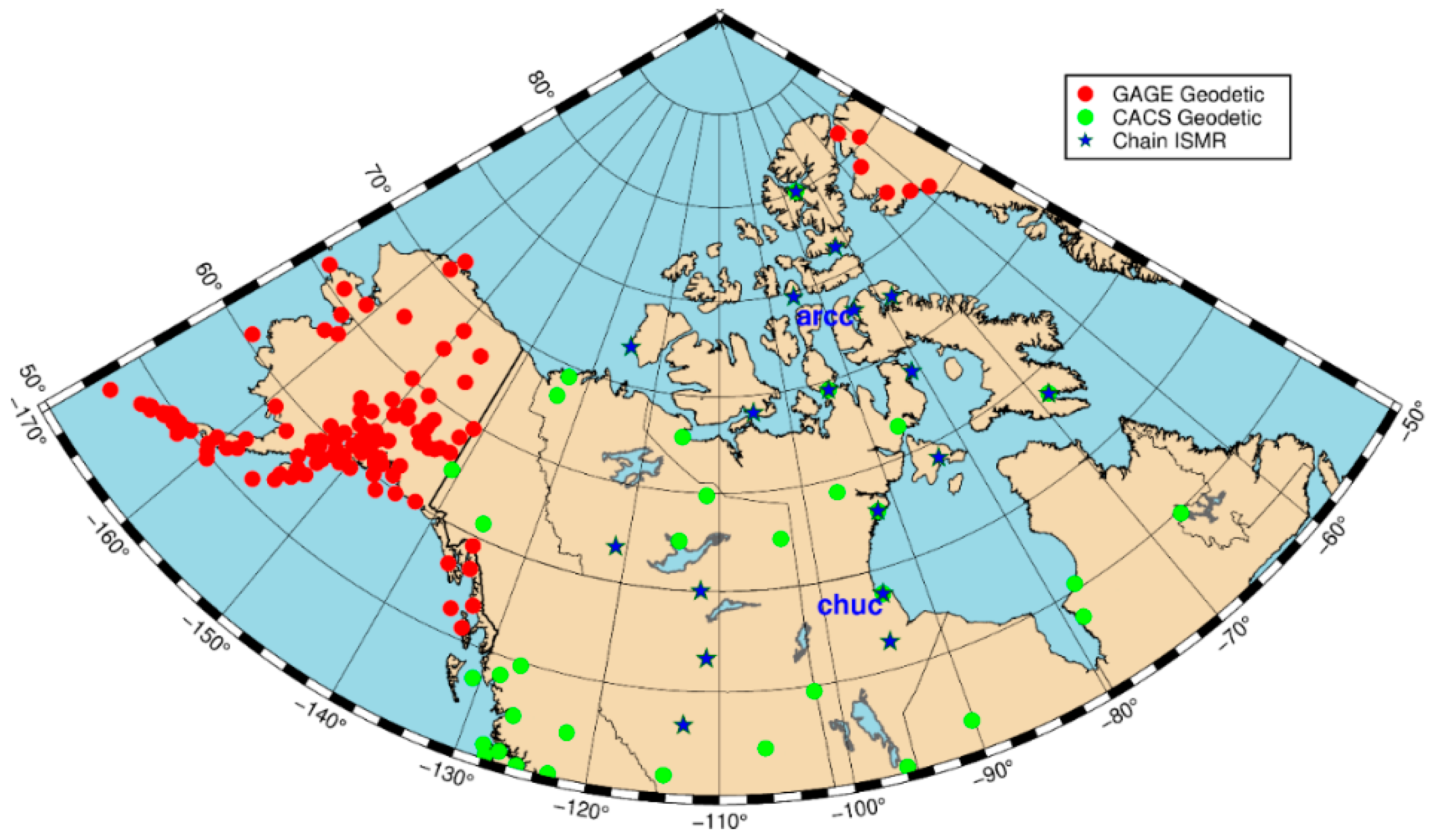
3. Introduction to the Adopted Data

Three types of data, including the in situ observations from Swarm satellites and the ground-based GNSS observations from both the ISMR receivers and the geodetic receivers, were adopted to analyze the accuracy of the 30s-sampling-interval scintillation indices in monitoring scintillations in the high-latitude regions. The ISMR observations were collected from 18 GNSS ionospheric scintillation and TEC monitors (GISTM) operated by the Canadian High Arctic Ionospheric Network (CHAIN). As displayed in Figure 1, these GISTM stations are located throughout the Canadian Arctic region, with the aim to understand the generation and dynamics of ionization structures with different scales in this region. Besides serving as the ISMR to log out the ${\sigma }_{\varphi }$ index, the GISTM can also be used as a normal dual-frequency GNSS receiver to provide the 30s-sampling-interval receiver independent exchange (RINEX) files, making it possible to compare the 30s-sampling-interval scintillation index with the ${\sigma }_{\varphi }$ index directly at the same station. The observations collected at all the 18 stations during the year of 2020 are adopted in this paper, while one high-latitude station arcc and one middle-latitude station chuc are used as examples to illustrate the accuracy of the 30s-sampling-interval scintillation indices in the time series. The geomagnetic coordinate of the station arcc is 81.85°N, 26.32°W, while that of the station chuc is 67.12°N, 29.29°W, which is close to the auroral oval.

The ground-based geodetic GNSS observations were collected from the continuously operating networks of the Geodetic Facility for the Advancement of Geosciences (GAGE) and Canadian Active Control System (CACS) with the sampling interval of 30 s. Considering the interest research area of this paper is the high-latitude region of North America (>50°), 139 stations and 38 stations were selected from the GAGE and CACS, respectively, shown as the red and green dots in Figure 1. Compared to the ISMR, the geodetic receivers are much more widely distributed as shown in Figure 1, making them more suitable to study the spatial accuracy of the scintillations detected by the 30s-sampling-interval scintillation indices. The observations from all the above stations collected in the whole year of 2020 were used in the following analysis.

The in situ electron density observations were collected from a Swarm, a constellation with three identical satellites, operating on a polar low Earth orbit. Swarm A and C ran at an altitude of 470 km, while Swarm B flew at 520 km. Although there were differences in the operation latitude, the scintillation monitoring results of the three satellites were identical statistically. Considering that a Swarm was utilized to validate the spatial accuracy of the scintillations detected by the 30s-sampling-interval scintillation indices, the observations of Swarm A collected during the year of 2020 were adopted in this paper.

4. Performance of the 30s-Sampling-Interval Scintillation Indices in Monitoring Scintillations

This section will evaluate the performance of the two scintillation indices extracted from 30s-sampling-interval observations using long-term ground and in situ data. The accuracy of the 30s-sampling-interval scintillation indices were assessed from both the time and space aspects using the ${\sigma }_{\varphi }$ index from ground ISMR stations and RODI and $N_e$ as the references, respectively. The daily scintillation occurrence rate and its correlation with the space weather parameters was adopted to evaluate the accuracy of the 30s-sampling-interval scintillation indices in the time aspect, while the scintillation monitoring accuracy in the space aspect was assessed from one observation arc and statistical scintillation occurrence rate in the study region based on the Swarm A satellite.

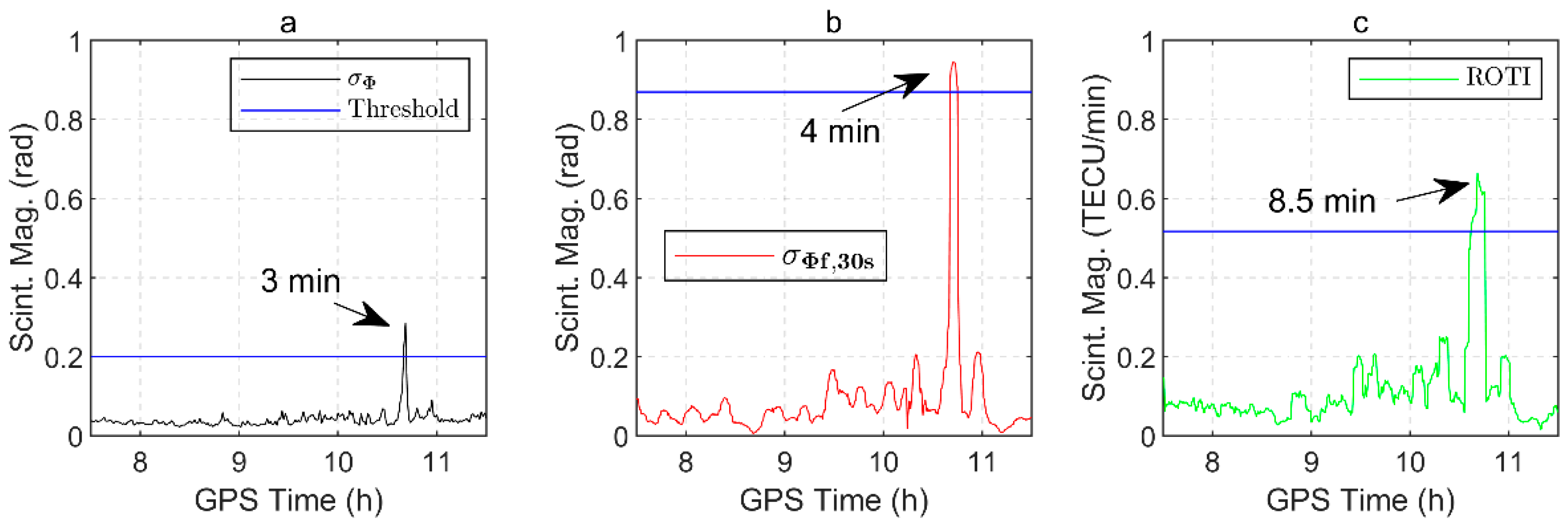
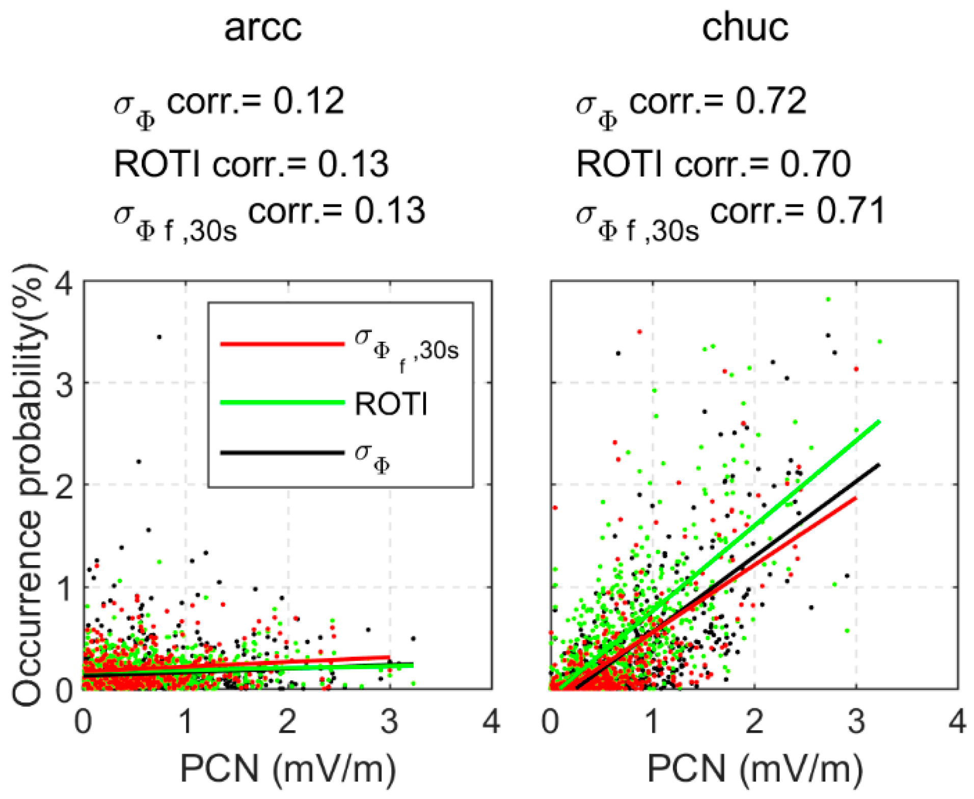
4.1. Analysis on the Accuracy of the 30s-Sampling-Interval Scintillation Indices in the Time Aspect

The accuracy of the two 30s-sampling-interval scintillation indices were firstly evaluated on account of the daily scintillation occurrence rate, which is defined as the number of epochs with scintillations above the total number of epochs in one day. The 30s-sampling-interval scintillation index can be considered as accurate if it can provide a consistent daily scintillation occurrence rate with the ${\sigma }_{\varphi }$ index obtained from the co-located ISMR. A proper scintillation threshold is needed to judge the occurrence of a scintillation, but compared to the ${\sigma }_{\varphi }$ index, the magnitude of the 30s-sampling-interval scintillation index was significantly different, leading to the inapplicability of the threshold of the ${\sigma }_{\varphi }$ index in these low-sampling-interval indices. The Complementary Cumulative Distribution Function (CCDF) method was used to determine the threshold of the 30s-sampling-interval scintillation indices [21], as follows. With the assumption that the 30s-sampling-interval indices can provide the same scintillation occurrence rate as the ${\sigma }_{\varphi }$ index in the whole year, the threshold for the 30s-sampling-interval indices can be determined as the magnitude corresponding to the percentile in the CCDF of the 30s-sampling-interval indices providing the same scintillation rate as the ${\sigma }_{\varphi }$ index. Based on the above CCDF method, the thresholds for the ${\sigma }_{\varnothing f,30s}$ index and ROTI were selected as 0.8693 rad and 0.5167 TECU/min at the station arcc, and 0.8008 rad and 0.2995 TECU/min at the station chuc, respectively. It should be noted that these thresholds were only determined to obtain a better scintillation monitoring performance based on the trial calculation. Although these thresholds are only valid at these two stations, they will not affect the following experiments and the conclusions for the following reason—these thresholds are only needed to determine the scintillation occurrence rate in the time series where only observations collected at these two stations are adopted, while the magnitude of the scintillation index is adopted in the space aspect where all the stations are used.

Figure 2 displays the scintillation detection performance of the ${\sigma }_{\varphi }$, ${\sigma }_{\varnothing f,30s}$ and ROTI indices with the selected thresholds on one observation arc. It shows that all three scintillation indices could detect the occurrence of scintillation; however, the durations of the scintillation given by the 30s-sampling-interval indices were longer than the ${\sigma }_{\varphi }$ index. Compared to the duration given by the ${\sigma }_{\varnothing f,30s}$ index, that provided by ROTI was much larger than the ${\sigma }_{\varphi }$ index, which might be due to the effect of the not-eliminated ionospheric refraction error. This result meets with our previous findings [12], where the rate of epochs with scintillations given by ROTI were larger than that given by the ${\sigma }_{\varphi }$ index due to the same reason. Another reason for the longer duration detected by the two 30s-sampling-interval-based scintillation indices could be the difference in the length of period used for calculating the indices. A duration of 60 s was adopted for the ${\sigma }_{\varphi }$ index, while the ${\sigma }_{\varnothing f,30s}$ and ROTI utilized 5 min. This figure also shows that low magnitude scintillations in the ${\sigma }_{\varphi }$ index, e.g., the arc during 9:00 to 10:00, can lead to violent fluctuations in the 30s-sampling-interval indices, which was the reason for selecting new thresholds for the two 30s-sampling-interval scintillation indices.

Panels a and b of Figure 3 show the daily scintillation occurrence rates in the whole year of 2020 at the stations’ arcc and chuc, respectively, while the scintillation occurrence rate differences between the 30s-sampling-interval scintillation index and the reference, namely, the ${\sigma }_{\varphi }$ index, are displayed in Panels c and d. It can be seen that the ${\sigma }_{\varnothing f,30s}$ index had a consistent scintillation occurrence rate with the reference at both high-latitude and middle-latitude stations. The ROTI can provide an accurate daily scintillation occurrence rate at the middle-latitude station, while that in the high-latitude station is obviously larger than the reference, leading to a clear positive skewness in the rate difference. The above results indicate that the ${\sigma }_{\varnothing f,30s}$ index might be more suitable to monitoring high-latitude scintillation than the ROTI, which meets with our previous findings [12]. The reason leading to the inaccurate scintillation monitoring performance of the ROTI might have been that the drastically varying ionospheric irregularities in the high-latitude region cause a drastic variation gradient of the slant total electron content measured by the ROTI, hence, larger scintillation alerts and less accuracy of the ROTI.

The accuracy of the 30s-sampling-interval scintillation indices in the time aspect was further evaluated on account of the correlation between the scintillation occurrence rate and the parameters of space weather, which is defined as the conditions on the sun and in the solar wind, magnetosphere, ionosphere, and thermosphere that can influence the performance and reliability of spaceborne and ground-based technological systems, and can endanger human life or health [36,37]. The electron content in the high-latitude region is highly vulnerable to the disturbance of space weather, hence generating ionospheric irregularities, which fluctuate the amplitude and the phase of the GNSS signals, resulting in scintillations [38,39]. The 30s-sampling-interval index can be considered as accurate if a similar correlation can be achieved compared to the reference.

Two types of factors, i.e., the Ap index and polar cap north (PCN) index, were adopted to characterize the disturbance of space weather. The Ap index reflects the solar particle radiation by its magnetic effects [40] with a time resolution of three hours. The PCN index can be used to measure the ionospheric condition in the high-latitude region by monitoring the polar cap magnetic activity generated by the geoeffective solar wind parameters.

Figure 4 displays the distribution of the daily scintillation occurrence rates with the daily averaged Ap index, while the correlations are also shown on the top of each panel. The linear fitted lines to the distribution using the least square principle are also displayed in each panel. Compared to the ROTI, the correlations and the slopes of the linear fitted lines obtained by the ${\sigma }_{\varnothing f,30s}$ index were closer to those given by the reference at both stations, although the differences were not obvious, indicating that the scintillation monitoring performance of the ${\sigma }_{\varnothing f,30s}$ index was better than the ROTI. It can also be seen from this figure that the correlations obtained by all the three types of scintillation indices at the high-latitude station were lower than those at the middle-latitude station.

Figure 5 shows the distribution of the daily scintillation rates with the daily averaged PCN index. Similar to the Ap index, the correlations obtained from all three types of scintillation indices at the high-latitude station were lower than those at the middle-latitude station, which could be reached at 0.7. Moreover, it can also be seen from the figure that the slope of the linear fitted line given by the ${\sigma }_{\varnothing f,30s}$ index at the middle-latitude station was better than that provided by the ROTI compared to the reference, indicating the advantages of the ${\sigma }_{\varnothing f,30s}$ index, especially at the station chuc. The corresponding probability values for all the correlations in both Figure 4 and Figure 5 were lower than the significance level of 0.05, indicating the rejection of the null hypothesis, namely, that a correlation exists between the scintillation indices and the space weather parameters, although some correlations were weak.

The existing research has proved that the scintillation occurrence rate is highly dependent on the local time [22]. The ability to detect this local-time-dependent scintillation variation pattern can be used to evaluate the accuracy of the 30s-sampling-interval scintillation index. The local time was calculated based on the methods provided by Meeus [41], with regards to the atmospheric refraction correction. In order to reflect the impact of solar radiation on the ionosphere, the calculated local time refers to the height of the ionospheric pierce point, instead of the height of an antenna. According to the thin shell ionosphere model, the height of the ionosphere is assumed to be 470 km, which is the same altitude where the Swarm A satellite was operated. The calculated time does not change much if a slightly different ionosphere height is selected. The variation pattern of the ionospheric scintillation with the local time is illustrated by the scintillation occurrence rate per hour, i.e., the rate of epochs with scintillations in each hour.

Figure 6 displays the variation of the scintillation occurrence rate with the local time and day of the year 2020 at the stations’ arcc and chuc. As shown in the left two panels, the results of the ${\sigma }_{\varphi }$ index reveal that the occurrence of the scintillation was highly depended on the local time. Scintillations occur more often during local noon at a high-latitude station arcc, while the station chuc located close to the auroral oval region witnesses the highest occurrence rate from the local sunset to around midnight. The intensity of the solar activity can be illustrated by the number of sunspots in each month. As shown in Figure 7, the solar activity was gradually increased in the year 2020, changing from the 24th solar cycle to the 25th. The scintillation occurrence rate might also be affected by the strength of solar activity [23], as revealed by the upper left panel of Figure 6.

Considering the scintillation occurrence patterns provided by the ${\sigma }_{\varphi }$ index, the two 30s-sampling-interval scintillation indices both provided similar patterns at the middle-latitude station chuc, while both the scintillation indices were not effective in detecting the above patterns at the high-latitude station arcc, as shown in the middle and right panels of Figure 6, as well as Figure 4 and Figure 5. Compared to the ${\sigma }_{\varnothing f,30s}$ index, the ROTI was less accurate in the high-latitude region, as incorrect scintillations could be detected nearly at any time of a day, as shown in the upper right panel, as well as Figure 3. This further illustrates that the ROTI is less effective in monitoring scintillations at high-latitude regions, which is consistent with our previous research results [12].

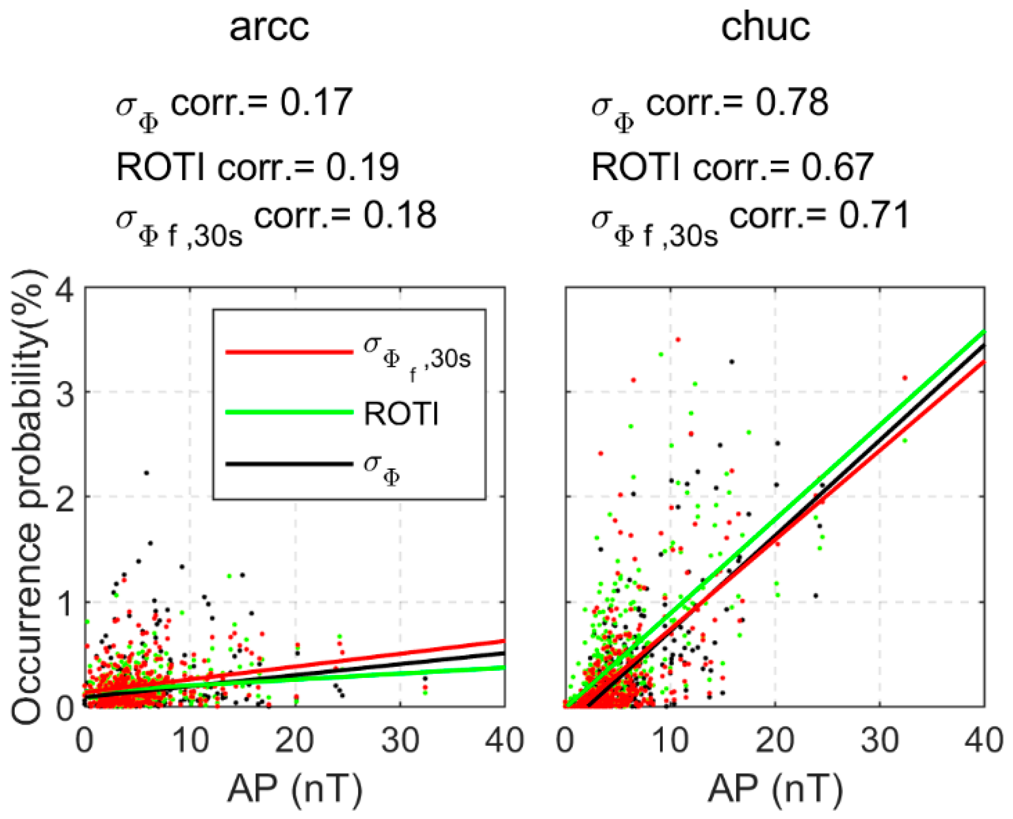
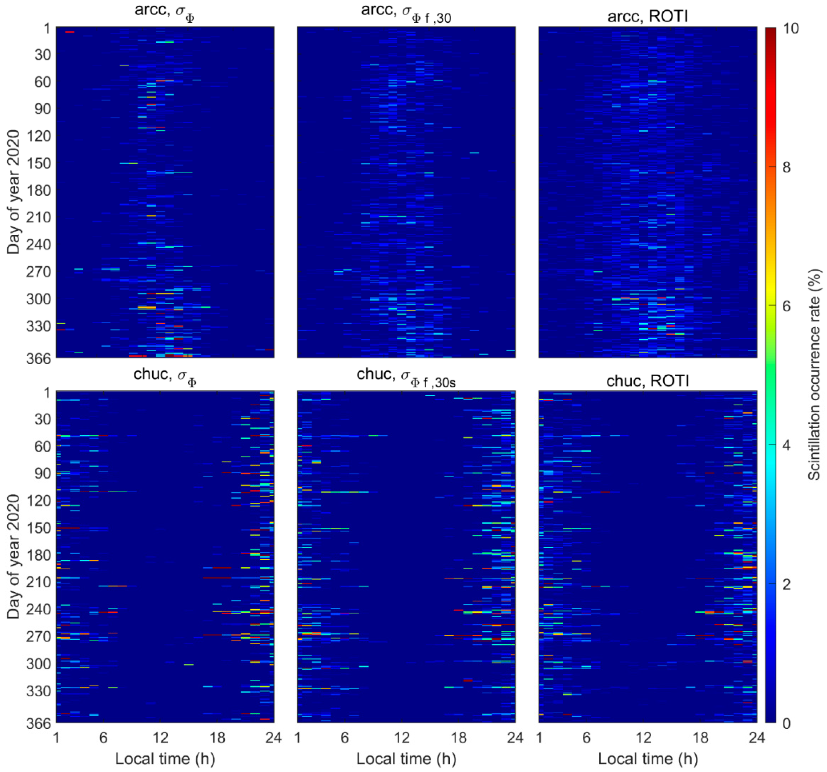
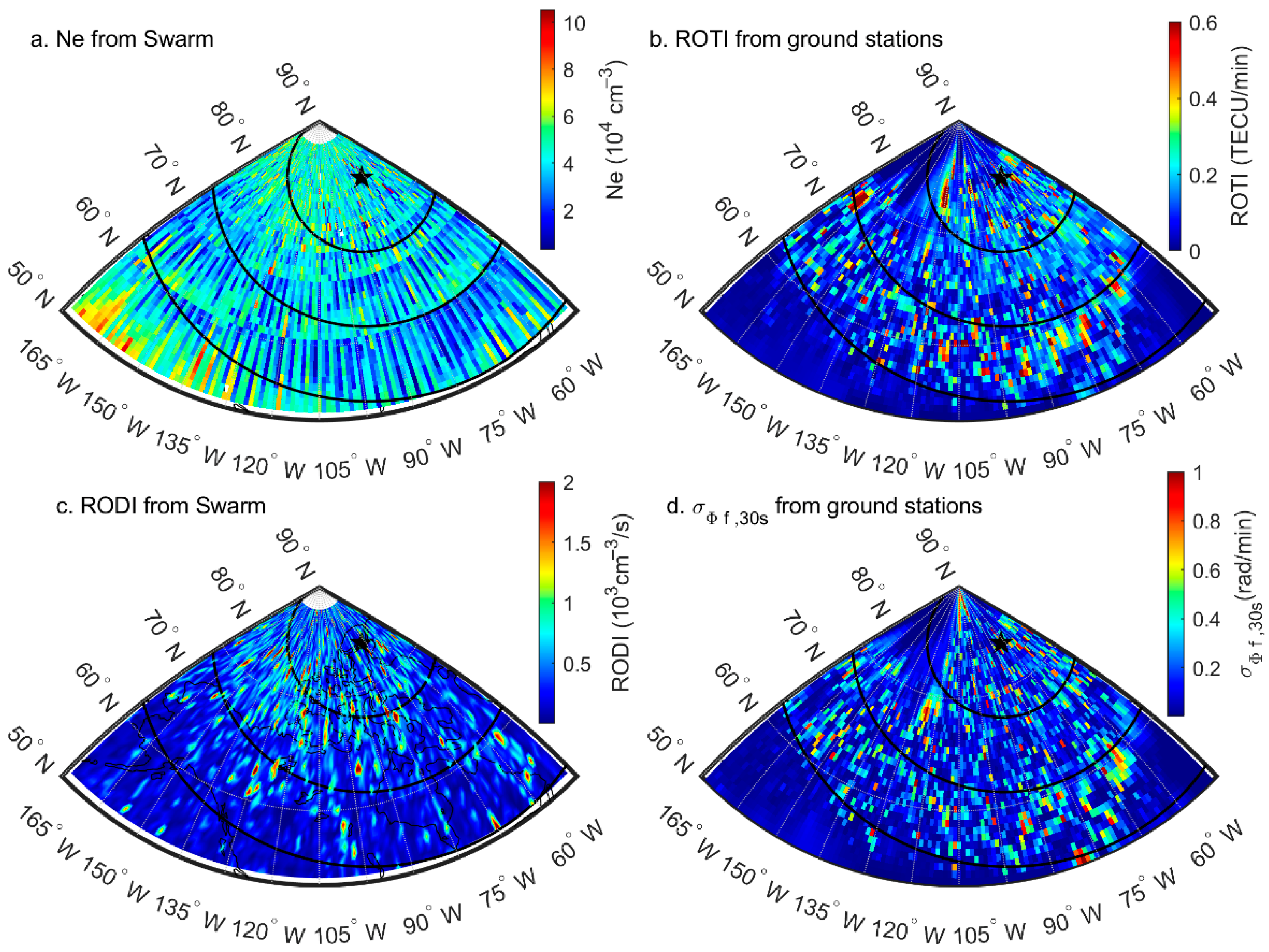
4.2. Analysis on the Accuracy of the 30s-Sampling-Interval Scintillation Indices in the Space Aspect

The performance of the 30s-sampling-interval scintillation index was evaluated by analyzing the accuracy in detecting the spatial distribution of the scintillations in a time span. Due to its sparse distribution, an ISMR is difficult to be used in detecting the spatial distribution of scintillations in a large area, while the densely distributed geodetic receivers make it possible to monitor the spatial distribution of ionospheric scintillations during a short period of time. This paper adopted the in situ observations of the Swarm A satellite to analyze the accuracy of the two 30s-sampling-interval scintillation indices in detecting the spatial distribution of scintillations, from the following two aspects. The first was to analyze the accuracy in detecting the scintillation pattern in one observation arc of the Swarm A satellite. The other was to analyze the statistical accuracy of the spatial distribution of scintillations in the year of 2020.

Figure 8 shows the comparison between the in situ observations of Swarm A and the cross-sectional scintillation index obtained from the grid model based on dense ground geodetic receivers. Panel a displays the arc of Swarm A, moving from a low latitude to the North Pole at 1:19–1:28 local time on 19 April 2020. This observation arc was located at the region between 85°W–116°W longitude and 50°N–85°N latitude. The covered region of this observation arc can be divided into three parts, i.e., the middle latitude, Auroral oval, and Polar cap, which was determined by detecting the field-aligned current (FAC) density [42], as the appearance of the FAC is highly related to the auroral oval. The FAC density was derived by the multiplication of the radial current (IRC) density with the inclination angle of the geomagnetic field using the observations from the vector magnetometer of Swarm A. The variation of the plasma density along the observation arc is displayed in Panel d. The plasma density was obtained directly from Langmuir probe files of Swarm A. Regarding the previous determined three regions, it can be seen from Panel d that the plasma density did not fluctuate widely in the middle-latitude region, although the magnitude was high, while significant variation was witnessed in the auroral oval region. The aurora is associated with significant particle precipitation and FACs from the magnetosphere, providing free energy for the development of ionospheric irregularities, hence, scintillations in the passing-through signals [43], as shown in Panel e. Some small-scale plasma density variations occurred in the polar cap region, which might have been due to the tiny polar cap patches, leading to scintillations with a small magnitude as well, as shown in Panels d and e.

In order to analyze the spatial accuracy of the 30s-sampling-interval scintillation index in the observation arc of Swarm A, a regional scintillation grid model was constructed using the 30s-sampling-interval observations collected at all the stations listed in Figure 1 during the observation period of Swarm A. Panels b and c show the scintillation grid model of the ROTI and the ${\sigma }_{\varnothing f,30s}$ index, respectively, without considering the movement of the ionospheric irregularity, which can be neglected during such a short period. The scintillation grid model was built up with the following procedures. First, all the GNSS observations with the elevation angle above 30° were adopted to calculate the ionospheric scintillation indices, i.e., the ${\sigma }_{\varnothing f,30s}$ index and the ROTI, and the corresponding coordinates of the ionospheric pierce points. Then, the ionosphere was divided into grids with a resolution of 0.2 degrees for both the latitude and longitude at the height of the ionospheric pierce point. Lastly, the biharmonic spline interpolation (BSI) was adopted to construct the scintillation grid model based on the previous calculated scintillation indices, coordinates and grids [44]. The advantage of the BSI method is that it supports a two-dimension interpolation without triangulation.

The scintillation from the 30s-sampling-interval ground GNSS observation along the arc of Swarm A could be obtained by applying the interpolation method to the above scintillation grid models regarding the coordinates of Swarm A. Due to the high resolution of the above scintillation grid model, an acceptable accuracy could be achieved by applying a linear interpolation. Panels f and g display the interpolated ROTI and the ${\sigma }_{\varnothing f,30s}$ index along the arc of Swarm A. It can be seen that the ${\sigma }_{\varnothing f,30s}$ index and ROTI provided a consistent performance with the in situ observations in the middle-latitude and auroral oval region, which means that the scintillation in the auroral oval region was much stronger than that in the middle-latitude region. Slightly different scintillation monitoring performances were witnessed for the ${\sigma }_{\varnothing f,30s}$ index and ROTI in the polar cap region for the following reason. As shown in Panels b and c, the grid model results for the ROTI and ${\sigma }_{\varnothing f,30s}$ index in the polar cap region were of significant difference, due to the unavailability of ground GNSS observations in such a region. Although the inaccurate model in the no-data region distorted the interpolation results of the ROTI and the ${\sigma }_{\varnothing f,30s}$ index, the overall fluctuation trends for both scintillation indices were consistent, indicating the accuracy of the 30s-sampling-interval scintillation indices in the space aspect.

The spatial accuracy of the 30s-sampling-interval scintillation index was further evaluated with all the in situ observations of Swarm A in the whole research region during the year 2020, as shown in Figure 9. The research region was divided into grids with a spatial resolution of 0.2 degrees in both the latitudes and longitudes. Then the BSI method was applied to obtain the statistical grid model of the plasma density and RODI from Swarm A in the whole year of 2020, as shown in Panels a and c, respectively. The ROTI and the ${\sigma }_{\varnothing f,30s}$ index grid models in the research region were also constructed using all the ground GNSS observations with the BSI method, as shown in Panels b and d, respectively. The black arcs in each panel represent the geomagnetic latitudes in a cadence of 10 degrees, while the black star stands for the geomagnetic north pole. The geomagnetic latitudes were calculated using the International Geomagnetic Reference Field (IGRF-13) model [45]. As shown in Panels a and c, the statistical results of the plasma density and RODI of Swarm A revealed that the middle latitude region, which was lower than the geomagnetic latitude of 60°, had a higher plasma density, while the ionospheric irregularities occurred more frequently at the geomagnetic polar pole, namely, the open geomagnetic area. Panels b and d display that the ionospheric scintillations provided by the ground GNSS observations were concentrated in the region above the geomagnetic latitude of 60°, especially within the geomagnetic latitude circle at 80°, although a random distribution pattern could be observed. A little inconsistency between the statistical scintillation monitoring performance of Swarm A and the ground GNSS receivers might be due to the different observation geometry. The plasma density and RODI were taken from the in situ observations of Swarm A at about 470 km, while the ROTI and the ${\sigma }_{\varnothing f,30s}$ index were calculated based on the integration from the ground to the GNSS satellites, causing the observations to contain plasma that was not necessarily along the same magnetic flux tube. The line-of-sight (LOS) direction is also one of the key factors to determine the magnitude of the scintillation indices based on ground GNSS receivers. Due to the limitations of orbit inclination angles, most GNSS satellites cannot reach high-latitude regions, making it so that no truly field aligned LOS can be observed in the high-latitude region, while high-latitude magnetic field lines are approximately radial. Moreover, the ground-based GNSS scintillation indices are affected by E-layer disturbances, which cannot be detected by the in situ observations of Swarm satellites. Park et al. provides a detailed discussion on the magnitude of scintillations observed by different geometries of the GNSS LOS direction with respect to in situ observations [18].

5. Conclusions

The accuracy of the scintillation monitoring performance in the high-latitude region using two 30s-sampling-interval scintillation indices were studied in both time and space aspects, with the phase scintillation index from an ISMR and the in situ observations from Swarm A as the references. The accuracy of the 30s-sampling-interval scintillation indices in the time aspect was analyzed in the following three-pronged approaches, i.e., the accuracy of the daily scintillation occurrence rates in the year 2020, the correlation with two space weather parameters, and the variation pattern of the scintillation occurrence with the local time and day of the year 2020. From the research results of the time accuracy, it can be seen that the performance of both 30s-sampling-interval scintillation indices met better with the reference at the middle-latitude station than that at the high-latitude station, where the accuracy of the ${\sigma }_{\varnothing f,30s}$ index performed better than the ROTI. As confirmed by the results of the daily scintillation occurrence rate and the variation pattern with local time at the high-latitude station, the results achieved by the ROTI were obviously greater than those given by the reference, indicating that the ROTI might not be reliable in high-latitude regions, which is consistent with previous research conclusions [12]. The poor performance of the ROTI in high-latitude regions might be due to the rapid drift characteristics of ionospheric irregularities in the polar region and the insufficient error elimination of the geometry-free method used in calculating the ROTI.

The accuracy of the two 30s-sampling-interval scintillation indices was further analyzed with the two parameters from the Swarm A satellite as the references, i.e., the plasma density and RODI. The performance of both 30s-sampling-interval scintillation indices in the space aspect was studied in the following two-pronged approaches, i.e., the scintillation monitoring performance in a Swarm A observation arc, and the statistical scintillation occurrence in the whole research region throughout the year 2020. Due to the distribution limitation of GNSS satellites, it was impossible to obtain the space-continuous scintillation monitoring performance directly from the GNSS observations. For this reason, this paper constructed the scintillation grid model based on the biharmonic spline interpolation method, hence, obtaining the scintillation indices of the ground observations on the arc of Swarm A with interpolation. From the scintillation monitoring results on the arc of Swarm A, both 30s-sampling-interval scintillation indices provided a consistent performance with the references in the middle-latitude and auroral oval regions, while the performance of the ROTI was less reliable than that of the ${\sigma }_{\varnothing f,30s}$ index, indicating the inapplicability of the ROTI in the polar region. Both the scintillation indices can provide similar scintillation monitoring results based on the statistical space distribution of the scintillations, which concentrate in the region with a geomagnetic latitude over 60 degrees.

Overall, considering the efficiency of both 30s-sampling-interval scintillation indices in monitoring scintillations and detecting the occurrence patterns in both time and space aspects, it is reasonable to believe that the scintillation index extracted from 30s-sampling-interval ground-based GNSS receivers can be used in scintillation monitoring research; however, it is also worth noting that the 30s sampling interval made it difficult to extract scintillations with high frequencies and short durations, especially for the ROTI. Consequently, future research should deal with the errors caused by the reduction in the sampling interval accuracy, to further improve the extraction accuracy of the ionospheric scintillation indices; thus, a more accurate two-dimensional scintillation grid model can then be constructed in the high-latitude region. By doing this, dense geodetic receivers can truly serve the prediction and early warning of the ionospheric scintillation in the high-latitude region. Moreover, the 30s-sampling-interval scintillation indices were validated with observations collected in a solar minimum year in this paper, but although the solar activity increased in the end of year 2020, the amount of data was not enough to fully test the effectiveness of the scintillation indices under strong solar activity. More experiments, with more observations collected with higher geomagnetic and solar activities, are left for future research.

References

1. Aarons, J. Global morphology of ionospheric scintillations. Proc. IEEE 1982, 70, 360–378. [Google Scholar] [CrossRef]
2. Béniguel, Y.; Cherniak, I.; Garcia-Rigo, A.; Hamel, P.; Hernández-Pajares, M.; Kameni, R.; Kashcheyev, A.; Krankowski, A.; Monnerat, M.; Nava, B. MONITOR Ionospheric Network: Two case studies on scintillation and electron content variability. Ann. Geophys. 2017, 35, 377–391. [Google Scholar] [CrossRef]
3. Vani, B.C.; Shimabukuro, M.H.; Galera Monico, J.F. Visual exploration and analysis of ionospheric scintillation monitoring data: The ISMR Query Tool. Comput. Geosci. 2017, 104, 125–134. [Google Scholar] [CrossRef]
4. Jayachandran, P.; Langley, R.; MacDougall, J.; Mushini, S.; Pokhotelov, D.; Hamza, A.; Mann, I.; Milling, D.; Kale, Z.; Chadwick, R. Canadian high arctic ionospheric network (CHAIN). Radio Sci. 2009, 44, 1–10. [Google Scholar] [CrossRef]
5. Wu, Z.; Wang, Q.; Hu, C.; Yu, Z.; Wu, W. Modeling and assessment of five-frequency BDS precise point positioning. Satell. Navig. 2022, 3, 8. [Google Scholar] [CrossRef]
6. Juan, J.M.; Aragon-Angel, A.; Sanz, J.; González-Casado, G.; Rovira-Garcia, A. A method for scintillation characterization using geodetic receivers operating at 1 Hz. J. Geod. 2017, 91, 1383–1397. [Google Scholar] [CrossRef]
7. Juan, J.M.; Sanz, J.; Rovira-Garcia, A.; González-Casado, G.; Ibáñez, D.; Perez, R.O. AATR an ionospheric activity indicator specifically based on GNSS measurements. J. Space Weather Space Clim. 2018, 8, A14. [Google Scholar] [CrossRef]
8. Nguyen, V.K.; Rovira-Garcia, A.; Juan, J.M.; Sanz, J.; González-Casado, G.; La, T.V.; Ta, T.H. Measuring phase scintillation at different frequencies with conventional GNSS receivers operating at 1 Hz. J. Geod. 2019, 93, 1985–2001. [Google Scholar] [CrossRef]
9. Ahmed, A.; Tiwari, R.; Strangeways, H.; Dlay, S.; Johnsen, M. Wavelet-based analogous phase scintillation index for high latitudes. Space Weather 2015, 13, 503–520. [Google Scholar] [CrossRef]
10. Zhao, D.; Li, W.; Li, C.; Tang, X.; ZHANG, K. Extracting an ionospheric phase scintillation index based on 1 Hz GNSS observations and its verification in the Arctic region. Acta Geod. Cartogr. Sin. 2021, 50, 368–383. [Google Scholar] [CrossRef]
11. Olwendo, J.O.; Cilliers, P.; Weimin, Z.; Ming, O.; Yu, X. Validation of ROTI for ionospheric amplitude scintillation measurements in a low-latitude region over Africa. Radio Sci. 2018, 53, 876–887. [Google Scholar] [CrossRef]
12. Zhao, D.; Li, W.; Li, C.; Hancock, C.M.; Roberts, G.W.; Wang, Q. Analysis on the ionospheric scintillation monitoring performance of ROTI extracted from GNSS observations in high-latitude regions. Adv. Space Res. 2022, 69, 142–158. [Google Scholar] [CrossRef]
13. Kivanç, Ö.; Heelis, R.A. Structures in ionospheric number density and velocity associated with polar cap ionization patches. J. Geophys. Res. Space Phys. 1997, 102, 307–318. [Google Scholar] [CrossRef]
14. Coley, W.R.; Heelis, R.A. Seasonal and universal time distribution of patches in the northern and southern polar caps. J. Geophys. Res. Space Phys. 1998, 103, 29229–29237. [Google Scholar] [CrossRef]
15. Chartier, A.T.; Mitchell, C.N.; Miller, E.S. Annual Occurrence Rates of Ionospheric Polar Cap Patches Observed Using Swarm. J. Geophys. Res. Space Phys. 2018, 123, 2327–2335. [Google Scholar] [CrossRef]
16. Goodwin, L.V.; Iserhienrhien, B.; Miles, D.M.; Patra, S.; Van der Meeren, C.; Buchert, S.C.; Burchill, J.K.; Clausen, L.B.N.; Knudsen, D.J.; McWilliams, K.A.; et al. Swarm in situ observations of F region polar cap patches created by cusp precipitation. Geophys. Res. Lett. 2015, 42, 996–1003. [Google Scholar] [CrossRef]
17. Spicher, A.; Cameron, T.; Grono, E.M.; Yakymenko, K.N.; Buchert, S.C.; Clausen, L.B.N.; Knudsen, D.J.; McWilliams, K.A.; Moen, J.I. Observation of polar cap patches and calculation of gradient drift instability growth times: A Swarm case study. Geophys. Res. Lett. 2015, 42, 201–206. [Google Scholar] [CrossRef]
18. Park, J.; Lühr, H.; Kervalishvili, G.; Rauberg, J.; Stolle, C.; Kwak, Y.-S.; Lee, W.K. Morphology of high-latitude plasma density perturbations as deduced from the total electron content measurements onboard the Swarm constellation. J. Geophys. Res. Space Phys. 2017, 122, 1338–1359. [Google Scholar] [CrossRef]
19. Jin, Y.; Spicher, A.; Xiong, C.; Clausen, L.B.N.; Kervalishvili, G.; Stolle, C.; Miloch, W.J. Ionospheric Plasma Irregularities Characterized by the Swarm Satellites: Statistics at High Latitudes. J. Geophys. Res. Space Phys. 2019, 124, 1262–1282. [Google Scholar] [CrossRef]
20. Pi, X.; Mannucci, A.J.; Lindqwister, U.J.; Ho, C.M. Monitoring of global ionospheric irregularities using the Worldwide GPS Network. Geophys. Res. Lett. 1997, 24, 2283–2286. [Google Scholar] [CrossRef]
21. Zhao, D.; Li, W.; Li, C.; Tang, X.; Wang, Q.; Hancock, C.M.; Roberts, G.W.; Zhang, K. Ionospheric Phase Scintillation Index Estimation Based on 1 Hz Geodetic GNSS Receiver Measurements by Using Continuous Wavelet Transform. Space Weather 2022, 20, e2021SW003015. [Google Scholar] [CrossRef]
22. Priyadarshi, S.; Zhang, Q.; Ma, Y.; Xing, Z.; Hu, Z.; Li, G. The Behaviors of Ionospheric Scintillations Around Different Types of Nightside Auroral Boundaries Seen at the Chinese Yellow River Station, Svalbard. Front. Astron. Space Sci. 2018, 5, 26. [Google Scholar] [CrossRef]
23. Zhao, D.; Li, W.; Wang, Q.; Liu, X.; Li, C.; Hancock, C.M.; Roberts, G.W.; Zhang, K. Statistical study on the characterization of phase and amplitude scintillation events in the high-latitude region during 2014–2020 based on ISMR. Adv. Space Res. 2022, 69, 3435–3459. [Google Scholar] [CrossRef]
24. Forte, B.; Radicella, S.M. Problems in data treatment for ionospheric scintillation measurements. Radio Sci. 2002, 37, 1–5. [Google Scholar] [CrossRef]
25. Forte, B. Optimum detrending of raw GPS data for scintillation measurements at auroral latitudes. J. Atmos. Sol. Terr. Phys. 2005, 67, 1100–1109. [Google Scholar] [CrossRef]
26. Spicher, A.; Clausen, L.B.N.; Miloch, W.J.; Lofstad, V.; Jin, Y.; Moen, J.I. Interhemispheric study of polar cap patch occurrence based on Swarm in situ data. J. Geophys. Res. Space Phys. 2017, 122, 3837–3851. [Google Scholar] [CrossRef]
27. Zhao, D.; Hancock, C.M.; Roberts, G.W.; Jin, S. Cycle Slip Detection during High Ionospheric Activities Based on Combined Triple-Frequency GNSS Signals. Remote Sens. 2019, 11, 250. [Google Scholar] [CrossRef]
28. Zhao, D.; Roberts, G.W.; Hancock, C.M.; Lau, L.; Bai, R. A triple-frequency cycle slip detection and correction method based on modified HMW combinations applied on GPS and BDS. GPS Solut. 2019, 23, 22. [Google Scholar] [CrossRef]
29. Wu, J.-T.; Wu, S.C.; Hajj, G.A.; Bertiger, W.I.; Lichten, S.M. Effects of antenna orientation on GPS carrier phase. In Astrodynamics 1991, Proceedings of the AAS/AIAA Astrodynamics Conference, Durango, CO, 19–22 August 1991; Univelt, Inc.: San Diego, CA, USA, 1992; pp. 1647–1660. [Google Scholar]
30. Beard, R.; Senior, K. Clock. In Springer Handbook of Global Navigation Satellite Systems; Springer: Cham, Switzerland, 2017; pp. 121–164. [Google Scholar]
31. Lagler, K.; Schindelegger, M.; Böhm, J.; Krásná, H.; Nilsson, T. GPT2: Empirical slant delay model for radio space geodetic techniques. Geophys. Res. Lett. 2013, 40, 1069–1073. [Google Scholar] [CrossRef]
32. Zhang, B.; Chen, Y.; Yuan, Y. PPP-RTK based on undifferenced and uncombined observations: Theoretical and practical aspects. J. Geod. 2019, 93, 1011–1024. [Google Scholar] [CrossRef]
33. Zhang, B.; Hou, P.; Zha, J.; Liu, T. Integer-estimable FDMA model as an enabler of GLONASS PPP-RTK. J. Geod. 2021, 95, 91. [Google Scholar] [CrossRef]
34. Olhede, S.C.; Walden, A.T. Generalized Morse wavelets. IEEE Trans. Signal Process. 2002, 50, 2661–2670. [Google Scholar] [CrossRef]
35. Liu, L.; Su, X.; Wang, G. On Inversion of Continuous Wavelet Transform. Open J. Stat. 2015, 5, 714–720. [Google Scholar] [CrossRef]
36. Sharma, G. Manifestation of earthquake preparation zone in the ionosphere before 2021 Sonitpur, Assam earthquake revealed by GPS-TEC data. Geod. Geodyn. 2022, 13, 230–237. [Google Scholar] [CrossRef]
37. Khazanov, G.V. Space Weather Fundamentals, 1st ed.; CRC Press: Boca Raton, FL, USA, 2016. [Google Scholar]
38. Eshkuvatov, H.E.; Ahmedov, B.J.; Tillayev, Y.A.; Tariq, M.A.; Shah, M.A.; Liu, L. Ionospheric precursors of strong earthquakes observed using six GNSS stations data during continuous five years (2011–2015). Geod. Geodyn. 2022. [Google Scholar] [CrossRef]
39. Maltseva, O.; Nikitenko, T. The effect of space weather on the ionosphere at the 110° meridian during CAWSES-II period. Geod. Geodyn. 2021, 12, 93–101. [Google Scholar] [CrossRef]
40. Matzka, J.; Stolle, C.; Yamazaki, Y.; Bronkalla, O.; Morschhauser, A. The geomagnetic Kp index and derived indices of geomagnetic activity. Space Weather 2021, 19, e2020SW002641. [Google Scholar] [CrossRef]
41. Meeus, J. Astronomical Algorithms, 2nd ed.; Willmann-Bell, Inc.: Cambridge, MA, USA, 1998. [Google Scholar]
42. Xiong, C.; Lühr, H. An empirical model of the auroral oval derived from CHAMP field-aligned current signatures—Part 2. Ann. Geophys. 2014, 32, 623–631. [Google Scholar] [CrossRef]
43. Jin, Y.; Moen, J.I.; Miloch, W.J.; Clausen, L.B.; Oksavik, K. Statistical study of the GNSS phase scintillation associated with two types of auroral blobs. J. Geophys. Res. Space Phys. 2016, 121, 4679–4697. [Google Scholar] [CrossRef]
44. Deng, X.; Tang, Z. Moving Surface Spline Interpolation Based on Green’s Function. Math. Geosci. 2011, 43, 663–680. [Google Scholar] [CrossRef]
45. Alken, P.; Thébault, E.; Beggan, C.D.; Amit, H.; Aubert, J.; Baerenzung, J.; Bondar, T.N.; Brown, W.J.; Califf, S.; Chambodut, A.; et al. International Geomagnetic Reference Field: The thirteenth generation. Earth Planets Space 2021, 73, 49. [Google Scholar] [CrossRef]
Figure 1. Distribution of the selected ground-based GNSS stations.
Remotesensing 14 04255 g001
Figure 2. Scintillation detection performance of the σ ϕ (a), σ f , 30 s (b) and ROTI (c) indices on the observation arc of PRN 32 at station arcc on the 111th day of year 2020. The “Scint. Mag.” in the y label stands for the scintillation magnitude.
Remotesensing 14 04255 g002
Figure 3. Daily scintillation occurrence rates in the year 2020 at stations arcc (a) and chuc (b). The rate differences between ROTI and σ ϕ at stations arcc and chuc are shown in panels (c) and (e) respectively, while those between σ ϕ f , 30 s and σ ϕ at stations arcc and chuc are displayed in panels (d) and (f).
Remotesensing 14 04255 g003
Figure 4. Correlation between the daily scintillation occurrence rate and the Ap index. The “corr.” denotes correlation.
Remotesensing 14 04255 g004
Figure 5. Correlation between the daily scintillation occurrence rate and the PCN index.
Remotesensing 14 04255 g005
Figure 6. Local time and seasonal dependency analysis of the ionospheric scintillation occurrence rate.
Remotesensing 14 04255 g006
Figure 7. Number of sunspots in each month of year 2020.
Remotesensing 14 04255 g007
Figure 8. Scintillation monitoring performance of the grid model constructed with the 30s-sampling-interval scintillation indices along an observation arc of Swarm A. (a) Observation arc of Swarm A in the research region, with timestamps, (b,c) the scintillation grid model based on the ground geodetic GNSS observations during the period of the observation arc of Swarm A, (d) the in situ plasma density from Swarm A, (e) the in situ RODI from Swarm A, (f) the variation of ROTI along the observation arc of Swarm A and (g) the variation of the σ f , 30 s index along the observation arc of Swarm A. The ionosphere region flags 1, 2 and 3 represent the middle latitudes, the auroral oval and the polar cap region, respectively.
Remotesensing 14 04255 g008
Figure 9. Statistical analysis on the scintillation monitoring performance of Swarm A (Panels (a,c)) and the ground GNSS geodetic receivers (Panels (b,d)) in the whole year of 2020.
Remotesensing 14 04255 g009
Publisher’s Note: MDPI stays neutral with regard to jurisdictional claims in published maps and institutional affiliations.