Abstract
Accurate bathymetric data is crucial for marine and coastal ecosystems. A lot of studies have been carried out for nearshore bathymetry using satellite data. The approach adopted extensively in shallow water depths estimation has recently been one of empirical models. However, the linear empirical model is simple and only takes limited band information at each bathymetric point into consideration. It may be not suitable for complex environments. In this paper, a deep learning framework was proposed for nearshore bathymetry (DL-NB) from ICESat-2 LiDAR and Sentinel-2 Imagery datasets. The bathymetric points from the spaceborne ICESat-2 LiDAR were extracted instead of in situ measurements. By virtue of the two-dimensional convolutional neural network (2D CNN), DL-NB can make full use of the initial multi-spectral information of Sentinel-2 at each bathymetric point and its adjacent areas during the training. Based on the trained model, the bathymetric maps of several study areas were produced including the Appalachian Bay (AB), Virgin Islands (VI), and Cat Island (CI) of the United States. The performance of DL-NB was evaluated by empirical method, machine learning method and multilayer perceptron (MLP). The results indicate that the accuracy of the DL-NB is better than comparative methods can in nearshore bathymetry. After quantitative analysis, the RMSE of DL-NB could achieve 1.01 m, 1.80 m and 0.28 m in AB, VI and CI respectively. Given the same data conditions, the proposed method can be applied for high precise global scale and multitemporal nearshore bathymetric maps generation, which are beneficial to marine environmental change assessment and conservation.
1. Introduction
The nearshore areas are vital to both humans and ecology. They provide an important resource for human productive life; hence, they are valued by the military forces of all countries. Accurate bathymetric maps are of economic value and importance to human activities such as sailing navigation, fishing, coastal planning, etc. The commonly used methods of bathymetry include passive and active bathymetry [1].
Light Detection and Ranging (LiDAR) is an active method extensively used for bathymetry. It can actively detect the spatial information of underwater features and then display the underwater environment in three dimensions through laser point clouds with very low error in the vertical direction. Traditional airborne LiDAR and shipborne LiDAR are highly accurate, high-density and short-period marine mapping technology recognized by mankind. Traditional airborne LiDAR and shipborne LiDAR would be unable to perform measurements due to the complex topography and harsh environment of the near-shore waters, as well as the inaccessibility of some of the shallower waters that are in dispute [2,3]. In situ measurements make airborne and shipborne bathymetry limited in certain areas. To break through this limitation, scholars have tried to use satellite-based LiDAR to obtain water depth information. A lot of studies have proved that satellite-based LiDAR can also obtain bathymetric points with enough accuracy through processing [4]. Consequently, this method is gradually becoming an alternative to in situ measurements for obtaining bathymetric information [5,6]. Although the problem of inaccessibility can be overcome with satellite-based LiDAR, the accuracy of the water depth from satellite-based LiDAR is difficult to ensure because the bathymetric pulse signals emitted by satellite-based LiDAR are subject to more interference over long distances and complex paths. Therefore, even though the LiDAR beam has a high penetration capacity underwater, it is essential to acquire further developments in bathymetry.
Compared with the active bathymetry method, optical depth inversion is a passive bathymetry method, which is based on the radiative transfer model. With the advantage in economic terms, global coverage and timeliness, remote sensing images are extensively adopted in nearshore bathymetry. The most commonly used images are Landsat and Sentinel-2 [7,8,9]. Based on these images, the main bathymetry approaches can be divided into two general classes: physical models and empirical models. Physics-based model inversion approaches can be used for bathymetry in the absence of known bathymetric points [10,11]. Gonzalo et al. [12] proposed a physical bathymetry inversion model by studying the wave frequency variation law. Inverting bathymetry through physical models not only misses many influences, but also lacks mathematical statistics [13,14]. Meanwhile, it is difficult to comprehensively estimate the factors for physical models; therefore, this method is difficult to use widely [15]. The empirical model makes use of the relationship between the radiation intensity of natural light and water depth. Because the radiation intensity of light is influenced by atmospheric conditions, water quality, etc. [16], known water depth data is required to calibrate the empirical model parameters [17]. Chen et al. [18] proposed a dual-band bathymetry method without bathymetric control points, which is difficult to implement and has low inversion accuracy. Kerr et al. [19] proposed a more accurate multispectral water depth inversion method. Later researchers proposed a physical model to extract bathymetry based on Gaussian regression statistics [20]. Bian et al. [21] inferred bathymetry by underwater photogrammetry. The regression kriging method [22] used multispectral remote sensing images and interpolated water depth data for bathymetry, which generated errors in the interpolation and leads to low accuracy of model inversion. Ma et al. [23] proposed a complex mathematical model for bathymetry inversion, but the model was not universal. Nevertheless, most of the empirical models do not take into account the spatial correlation between bathymetric points and surrounding pixels [24], and the traditional linear model is too simple to be suitable for complex environments.
At present, machine learning methods have attracted much attention due to their advantages in accepting high-dimensional features to build non-linear models [25,26,27,28]. Wang et al. [29] performed bathymetry using support vector machines considering spatial correlation. Sagawa et al. [30] gained bathymetry data using random forest. Wang et al. [31] employed a multi-layer perceptron which takes into account the different substrates for bathymetry. Wan et al. [32] proposed a deep learning network based on data perturbation for bathymetric inversion. Increasing a certain interference rate can increase the robustness of the model. However, this interference undoubtedly add artificial noise, resulting in low accuracy of bathymetric inversion. Bo Ai [33] combined the local connectivity properties of CNNs and local spatial correlation of water depth inversion image pixels to establish a model for remote sensing images and airborne LiDAR data. The results show that adding spatial information can improve the bathymetry accuracy; however, the method still relies on in situ measurements.
To summarize, prior research has thoroughly investigated the nearshore bathymetry from remote sensing data. The active-passive fusion inversion method has become a prevailing method for nearshore bathymetry. However, little research has been conducted to show the capability of the deep learning approach in bathymetry from remote sensing datasets. In the literature, a deep learning framework was proposed for nearshore bathymetry (DL-NB) from ICESat-2 LiDARand Sentinel-2 Imagery datasets. First, the bathymetric points from the spaceborne ICESat-2 LiDAR were extracted instead of in situ measurements. Then, the DL-NB made full use of the initial regional multi-spectral information of Sentinel-2 at each bathymetric point to train the model. Finally, based on the trained model, the bathymetric maps of selected study areas were produced including the Appalachian Bay (AB), Virgin Islands (VI), and Cat Island (CI) of the United States. To Evaluate the bathymetry accuracy of the proposed method, the traditional linear method [34], machine learning method [26] and multilayer perceptron (MLP) [35] were selected as the baseline.
2. Data
2.1. Sentinel-2 Data
There are abundant remote sensing image data sources for optical depth inversion; however, the sentinel-2 L2A data was selected as its following characteristics.
- The spatial resolution of 13 bands, including band 2 (blue), band 3 (green), band 4 (red), and band 8 (near-infrared) can reach 10 m, which provides the detailed characteristics of coastal areas where the seabed depth may be highly uneven.
- The 10 spectral bands selected in the study cover the range of 490–2190 nm, including the optical properties, depth, and spectral information of the bottom substrate (visible domain).
- L2A data is the surface reflectance data product obtained by the official atmospheric correction based on L1C. There is no need for other preprocessing. The cloud content of remote sensing images selected for water depth inversion is less than 1%, so there is no need for cloud removal.
The Appalachian Bay (AB), Virgin Islands (VI), and Cat Island (CI) of the United States were selected as the study areas. Table 1 lists the multispectral remote sensing image information of each study area.

Table 1.
Information of multispectral remote images.
True color images of these three areas, which represent benthic types (coral reefs, seagrasses, and sand), are shown in Figure 1, providing a completely independent evaluation of the models developed for the study.
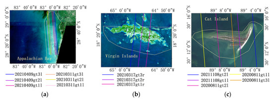
Figure 1.
Sentinel-2 true-color images of study areas. (a) Appalachian Bay. (b) Virgin Islands. (c) Cat Island. The colored lines in the figure are the ground track data of ICESat-2 used in the study.
2.2. Bathymetric Data
Both ICESat-2 and NOAA NGS Topobathy Lidar data were used in the study. The water depth points extracted from ICESat-2 were used as a priori data for network training. NOAA bathymetric points were used as the reference bathymetric points for accuracy assessment. ICESat-2 satellite-based LiDAR satellite provides us with an active remote sensing detection technology that uses 531 nm photon-counting LiDAR [36] with higher agility and underwater penetration capability. A diameter of 17 m per pulse and a spacing of 0.7 m along the track represent the spatial resolution of ICESat-2. After calibrating the bathymetric error and other errors, the spaceborne photon-counting LiDAR have a potential to achieve the bathymetric accuracy in shallow and clean water areas [6], and are capable of quantitatively obtaining shallow water depths. The bathymetric points of the nearshore were extracted from ICESat-2 for the model training. The Advanced Topographic Laser Altimeter System (ATLAS) [37] ATL03 disciplines information, and NOAA NGS Topobathy Lidar information used in this article were described in Table 2. Each ATLAS ATL03 data contains three groups (6 pieces) of ground track data: gt1l, gt1r, gt2l, gt2r, gt3l, and gt3r. Each group of data contains a strong information track and a weak information track. In this study, we only select strong information track data of each group to extract water depth.

Table 2.
Information of LiDAR data.
Topographic and bathymetric LiDAR data from the U.S. coastal islands provided by the NOAA Office of Coastal Management [38] was employed as verification bathymetric points. This LiDAR bathymetric data has the following characteristics:
- The vertical accuracy of the LiDAR in measuring shallow water areas can reach ((0.252) + (0.0075 × d)2) m under 95% confidence level (d is water depth); the vertical accuracy of the LiDAR in measuring deep water areas can reach ((0.302) + (0.013 × d)2) m under a 95% confidence level.
- The horizontal accuracy of the LiDAR can reach (3.5 + 0.05 × d) m at a 95% confidence level.
- The LiDAR data can be obtained free of charge and processed conveniently.
The verification bathymetric points of AB vary from 0 m to greater than 20 m. The verification bathymetric points of VI vary from 0 m to 35 m. Concurrently, the verification bathymetric points of CI range from 0 to 5 m.
3. Methods
3.1. Method Overview
The proposed method mainly includes the following steps. Firstly, bathymetric points were extracted from ICESat-2 ATLAS ATL03 data as the prior data. Then, the feature tensors were extracted from the registered Sentinel-2 images with a certain window size at each prior water depth point. Subsequently, the feature tensors were input into the depth learning framework (DL-NB) designed in this paper for model training. The airborne LiDAR data was used as validation data for performance evaluation. Finally, the large-scale bathymetric maps were generated. At the same time, a comparative analysis with baselines was performed.
3.2. Bathymetry from ICESat-2 ATL03
The bathymetric points were extracted from ICESat-2 ATL03 data instead of in situ measurements. The processing mainly consists of four steps:
- It is necessary to convert the point cloud from WGS84 ellipsoidal height to orthogonal height; this is because even though the length of the laser track in our study area is short, there is a tilt of the sea level in the ellipsoidal height.
- Noise filtering is implemented based on a two-dimensional window filter, with each point as the center, setting the window size and the point density threshold within the window to filter out discrete noise points. In most cases, the manual process is necessary.
- Sea level and seafloor determination are important to depth calculation. The sea level was determined based on histogram statistics at each points segment near the sea level, referring to two rules: 1. the points density of sea level is relatively high near the surface; 2. sea level is higher than seafloor.
- Refraction correction is performed on the seafloor points according to the algorithm proposed by Parrish et al. [6].
A schematic diagram of the ICESat-2 point cloud before and after processing is shown in Figure 2.
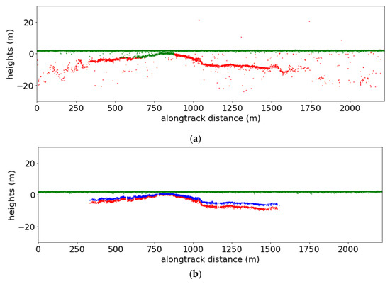
Figure 2.
Diagram of ICESat-2 before and after processing. (a) Pre-processing point cloud. (b) Point cloud after filtering and refraction correction. The green points represent the sea level, red points show the initial extracted seafloor topography, and the blue points show the refraction-corrected seafloor topography.
As can be seen from the above figure, after processing, the bathymetry value is calculated by differentiating the sea level and the refraction-corrected seafloor point clouds.
Assuming negligible changes in ocean bathymetry within a short period, the Sentinel-2 optical remote sensing images and airborne LiDAR data need to be matched in time. The tidal correction of the corresponding time on the Sentinel-2 optical remote sensing images should be considered [42,43], and the bathymetry values can be expressed as:
where is the image inversion bathymetry value, is the water depth after tidal correction by LiDAR, is the tidal height at the acquisition time of satellite-based LiDAR data (available in the .h5 file), is the tidal height at the acquisition time of Sentinel-2 optical remote sensing image, and the tide information of the corresponding tide stations in the study area can be viewed through the National Ocean Data Center for correction [44].
3.3. Deep Learning Architecture
CNN has shown its advantages in image recognition and classification, as well as regression analysis. In this paper, a 2D CNN-based deep learning framework was designed for bathymetric inversion. Its potential ability for bathymetric data estimation was evaluated. To train the model, the bathymetric point extracted from ICESat-2 should be registered with the pixel value in the sentinel-2 images. The pixel can be regarded as weighted averages of nearby known pixels. Hence, the method took into account the impact of adjacent pixels on water depth retrieval through 2D CNN.
Figure 3 shows the structure of the DL-NB. The role of the convolutional kernel of the CNN is to expand the feature, and the role of pooling is to reduce the width and height of the input image to make the model deeper. ReLU is the activation function, and the expression is shown as follows:
where is the input-independent variable and is the function value.
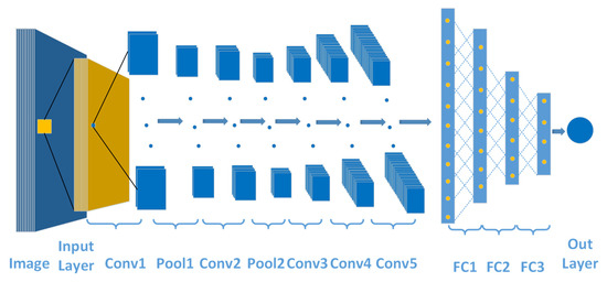
Figure 3.
2D CNN model (DL-NB) structure.
The neurons are adjusted nonlinearly after linear transformation, that is to say, the input vector from the previous layer of the neural network is transformed by and then output by transformation. Using the ReLU function can be more efficient than retrograde gradient descent and backward propagation, avoiding the problems of gradient explosion and gradient disappearance. The ReLU function is not affected by the complex activation function like the exponential function. The dispersion of activity can also reduce the overall computational cost of the neural network, which in turn simplifies the whole computational process [45]. In this paper, the most basic CNN was used, and the input layer was 10 neurons. We used the water depth points extracted from ICESat-2 as the a priori bathymetric points. At the same time, we extracted a 7 × 7 sub-image on the Sentinel-2 image (10 bands used in the study) with the a priori bathymetric point as the center. Feature tensors of size 10 × 7 × 7 (bands × width × height) were input into the network, whereas the depths of the priori bathymetric points were input into the network as labels for model training. The 2D CNN has a total of 5 layers, containing 64, 128, 256, 256, 512 neurons respectively. The output of each neuron was transferred to the input of the next neuron by the nonlinear activation function, and the activation functions of the hidden layers all adopted the ReLU function, which largely reduces the gradient disappearance. At last, the water depth was predicted by the linear activation function.
Backpropagation is the process used along with optimization methods to train the network [46], in which the weights in the network are updated according to the learning rate (α = 0.001) by calculating the gradient of the loss function and then using gradient descent for adaptive moment estimation (Adam, β1 = 0.9, β2 = 0.99), iterating continuously. When the iteration (epoch = 1000) stops and when the loss function converges at the same time the training of the model is completed.
3.4. Accuracy Assessment
To evaluate the performance of our trained model (DL-NB), several classic methods were employed as the baseline, including linear regression, MLP and Random Forest. The root means square error (RMSE) was calculated as an absolute metric. The smaller the RMSE, the higher the accuracy of the model. The RMSE expression is shown in formula 3.
Moreover, the coefficient of determination (R2) was employed to describe the model fitting effect; the value of R2 is in the range of [0, 1]; the larger the value, the better the model fitting effect. The expression is shown in formula 4.
N in the above equations denotes the sample size of test, is the estimated water depth, indicates the mean value of the estimated depth and is the corresponding depth from the NOAA airborne LiDAR data.
4. Model Results
4.1. Convolution Window Size Tuning
The convolution window size is important to the 2D CNN as well as the inversion accuracy. Considering the learning efficiency of the model, different window sizes were employed in Table 3. The result shows that the model (DL-NB) can achieve relatively high accuracy using the window size of 7 × 7 pixels. A window size too small or too large is not suitable for the model. Hence, the 7 × 7 window size was selected in our experiment.

Table 3.
Contrast experiment of different window sizes.
4.2. Bathymetry Maps of Models
Using the trained model and the pre-processed Sentinel-2 images, the nearshore bathymetric maps of three study areas were generated in Figure 4. Figure 4a–l correspond to the bathymetric maps derived from DL-NB, linear model, MLP and RF respectively. The comparison results show that there were clear visual differences between the results of DL-NB and the maps from the other models. The maps of DL-NB had richer details and better spatial continuity. The results from the linear model and the random forest show similar spatial distribution, while the maps of MLP show some differences, especially in the shallow areas of the Appalachian Bay.
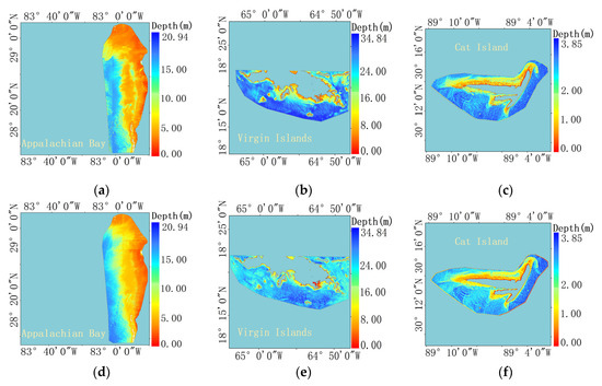
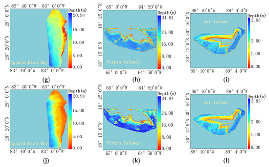
Figure 4.
Bathymetric maps of four study areas. (a–c) are the Bathymetric maps of Appalachian Bay, Virgin Islands, and Cat Island obtained through the DL-NB. (d–l) are acquired from linear regression, multilayer perceptron and random forest respectively.
4.3. Accuracy Analysis of Bathymetric Estimates
The correlation between the satellite-derived bathymetry (SDB) and in situ bathymetric points captured by the airborne LiDAR system was illustrated by scatter plots in each study area. As shown in Figure 5, the red line is the y = x line. Although the validate points are not evenly distributed, generally there is a strong correlation between the SDB and the in situ data. To further evaluate the performance of the DL-NB, R2 and RMSE between the retrieved water depths and in situ depths in three study areas were calculated and a comparison of accuracy with baselines were summarized in Table 4.

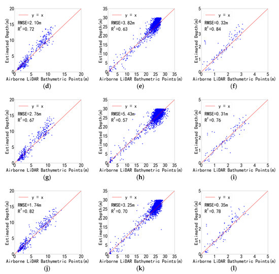
Figure 5.
Scatter plots drawn by the retrieved water depth values of the test sets and the water depth labels of the test sets in the four study areas. (a–c) are the scatter plots of Appalachian Bay, Virgin Islands, and Cat Island obtained through the DL-NB. (d–l) are acquired from linear regression, multilayer perceptron and random forest respectively.

Table 4.
Performance comparison of different models.
As shown in Table 4, the DL-NB can significantly outperform the baselines especially, in the Appalachian Bay and Virgin Islands. The RMSE of the Appalachian Bay improved by 173% overusing the MLP and the R2 improves from 67% to 93%. Similarly, the RMSE for the Virgin Islands improved by 202% overusing the MLP, and the R2 improved from 57% to 84%. Bathymetric inversions using the MLP had the worst accuracy in both the Appalachian Bay and the Virgin Islands. The LR and RF can achieve comparable performance.
5. Discussion
5.1. Error Analysis of SDB
The error of SDB in this paper mainly comes from Sentinel-2 image, the a priori water depth points extracted by ICESat-2, and in situ data provided by NOAA. Firstly, although the ICESat-2 ATL03 datasets were preprocessed to eliminate most of the errors during the prior water depth points extraction, the estimated refractive index of the water column will still lead to errors [47]. Besides, as shown in Figure 2, the filtered sea floor point cloud has a certain thickness, likely due to the noise or multi-path effect, which brings errors too. Secondly, atmospheric correction of Sentinel-2 images is essential for SDB; yet, sun glint and cloud may still persist after the correction and cause error [48]. Apart from that, the water quality, underwater topography and cover type in the study areas may affect the inversion accuracy of water depth as well [9,49,50,51]. Thirdly, it is difficult to maintain temporal synchronization for in situ data and other remote sensing data. Although the in situ data was employed as validation data, the accuracy of in situ data is affected by many factors such as geographical location, sea tidal and acquisition process [9].
5.2. Comparative Analysis of the Results of the Study Area
As can be seen from Table 4, the depth inversion accuracy of the DL-NB model is higher than the other three methods in each study area. Notably, another finding is that Cat Island has the highest accuracy, which is much higher than Virgin Islands. This may be explained by several reasons. One potential reason is that deeper water makes the water column more complex, and the inversion accuracy of the DL-NB model decreases with the increase of water depth. In addition, the water quality, underwater topography and cover types in different study areas are different. The underwater terrain of the Appalachian Bay is relatively flat, and the underwater cover of the Virgin Islands is more complex, which may affect the results of depth inversion as well.
5.3. Spatial Distribution of the Error
In order to deeply investigate the inversion methods, the error spatial distribution maps were generated by retrieved bathymetric maps and in situ DEM. As shown in Figure 6. Figure 6a–l correspond with the spatial distribution of bathymetric estimates error by different methods. Generally, there is no distinct rule in the error distribution. For DL-NB, the overestimation often happened in the shallow area of Appalachian Bay, and the underestimation always occurred in the deep area of Appalachian Bay. However, the error distribution was opposite in the Virgin Islands with the same method. By comparison, the results of DL-NB had the smallest differences in each study area, while the other three models tended to largely deviate from the in situ data. In particular, the MLP had the largest deviation in the Virgin Islands, which was over 6.6 m in deep areas.
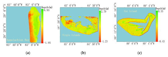
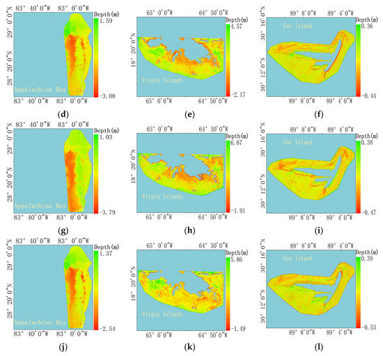
Figure 6.
Spatial distribution of bathymetric estimates error of different methods. (a–c) are the bathymetric maps of Appalachian Bay, Virgin Islands, and Cat Island obtained through the DL-NB. (d–l) are acquired from linear regression, multilayer perceptron and random forest respectively.
5.4. Model Portability
The data pre-processing is important to obtain a more accurate bathymetric map. Besides, there are many other factors affecting bathymetric results, including seawater turbidity, water column conditions and bottom type, etc. It makes sense to check the portability of the model in different environments. Based on the DL-NB, cross-validation was performed between the Virgin Islands and the Appalachian Bay. The DL-NB model was trained in one area and used in another. The validation result is shown in Table 5 indicates that the portability of the DL-NB model is poor. A possible reason is that there is great diversity in underwater terrain and coverage types among these areas, which will be reflected in the pixel values of remote sensing images. Figure 7 illustrates the average band value curves of 5 m and 10 m water depth in the same period of the US Appalachian Bay and the US Virgin Islands. There are great differences in the band values curve at a certain water depth in different study areas. Therefore, it is difficult to apply the trained model in one area to another different area for bathymetry.

Table 5.
Model portability test.
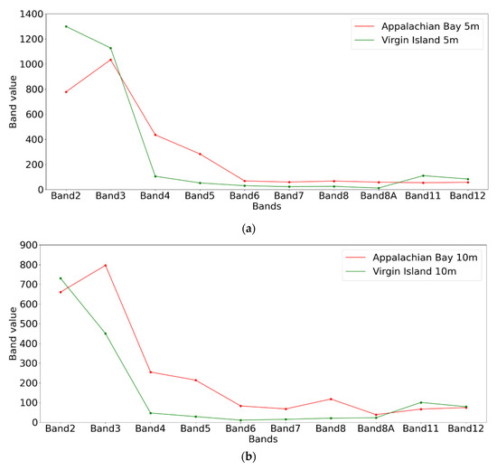
Figure 7.
Difference of average value in the same water depth band in different study areas. (a) average image band value of 5 m water depth. (b) average image band value of 10 m water depth.
6. Conclusions
In this study, a CNN-based deep learning framework was proposed for nearshore bathymetry (DL-NB). The bathymetric points from the spaceborne ICESat-2 lidar were extracted as the a priori measurement to train the DL-NB model with pre-processed sentinel-2 Images in selected study areas. Three classic methods were employed as baselines. The bathymetric maps, retrieved by different methods, show that the DL-NB model has richer details and better continuity visually.
To validate the performance of the proposed method, the inversion results were compared with in situ airborne LiDAR data from NOAA. The comparison suggested that the DL-NB model can outperform all the baselines, with the RMSE of 1.01, 1.8, 0.28 and the R2 of 0.93, 0.94, 0.82 in the three study areas respectively. RF can obtain a relatively higher accuracy than LR, and the performance of MLP was relatively poor. The results from different study areas also indicated that the uncertainty of accuracy increases with depth. Moreover, the spatial distribution of error was analyzed between the bathymetric maps and in situ data. It was found that, although there is no distinct rule in the error distribution, DL-NB had the smallest differences in each study area.
Finally, cross-validation was performed between different study areas to check the portability of DL-NB. The result indicate that the portability of the DL-NB model was poor in the study. It can be concluded that the diversity of environmental factors may limit the portability.
In the future, the proposed method can be tested by different remote sensing data and applied for high-precision global scale and multitemporal nearshore bathymetric map generation. These maps would be beneficial to marine environmental change assessment and conservation.
Author Contributions
Conceptualization, J.S.; Data Management, J.Z.; Capital Acquisition, J.S.; Survey, J.Z.; Methodology, J.Z.; Resources, J.Z.; Supervision, J.S.; Verification, J.Z.; Writing—Original Draft, J.Z.; Writing—Review and editing, J.S., Z.L. and Y.S. All authors have read and agreed to the published version of the manuscript.
Funding
This work was supported by the National Natural Science Foundation of China No.42171373.
Acknowledgments
The authors would like to thank the ESA’s Sentinel Scientific Data Hub for distributing the Sentinel-2 data, and the Goddard Space Flight Center for distributing the ICESat-2 data, besides, the authors also thank the editors and reviewers for their detailed comments and efforts toward improving the study.
Conflicts of Interest
The authors declare no conflict of interest. The authors declare that they have no known competing financial interests or personal relationships that could have appeared to influence the work reported in this paper.
References
- Su, H.; Liu, H.; Wang, L.; Filippi, A.M.; Heyman, W.D.; Beck, R.A. Geographically Adaptive Inversion Model for Improving Bathymetric Retrieval From Satellite Multispectral Imagery. IEEE Trans. Geosci. Remote Sens. 2013, 52, 465–476. [Google Scholar] [CrossRef]
- Schwarz, R.; Mandlburger, G.; Pfennigbauer, M.; Pfeifer, N. Design and Evaluation of a Full-Wave Surface and Bottom-Detection Algorithm for Lidar Bathymetry of Very Shallow Waters. ISPRS J. Photogramm. Remote Sens. 2019, 150, 1–10. [Google Scholar] [CrossRef]
- Janowski, Ł.; Tęgowski, J.; Nowak, J. Seafloor Mapping Based on Multibeam Echosounder Bathymetry and Backscatter Data Using Object-Based Image Analysis: A Case Study from the Rewal Site, the Southern Baltic. Oceanol. Nowak Hydrobiol. Stud. 2018, 47, 248–259. [Google Scholar] [CrossRef]
- Albright, A.; Glennie, C. Nearshore Bathymetry From Fusion of Sentinel-2 and ICESat-2 Observations. IEEE Geosci. Remote Sens. Lett. 2020, 18, 900–904. [Google Scholar] [CrossRef]
- Forfinski-Sarkozi, N.A.; Parrish, C.E. Analysis of MABEL Bathymetry in Keweenaw Bay and Implications for ICESat-2 ATLAS. Remote Sens. 2016, 8, 772. [Google Scholar] [CrossRef]
- Parrish, C.E.; Magruder, L.A.; Neuenschwander, A.L.; Forfinski-Sarkozi, N.; Alonzo, M.; Jasinski, M. Validation of ICESat-2 ATLAS Bathymetry and Analysis of ATLAS’s Bathymetric Mapping Performance. Remote Sens. 2019, 11, 1634. [Google Scholar] [CrossRef]
- Zhang, X.; Chen, Y.; Le, Y.; Zhang, D.; Yan, Q.; Dong, Y.; Han, W.; Wang, L. Nearshore Bathymetry Based on Icesat-2 and Multispectral Im-ages: Comparison between Sentinel-2, Landsat-8, and Testing Gaofen-2. IEEE J. Sel. Top. Appl. Earth Obs. Remote Sens. 2022, 15, 2449–2462. [Google Scholar] [CrossRef]
- Pacheco, A.; Horta, J.; Loureiro, C.; Ferreira, Ó. Retrieval of nearshore bathymetry from Landsat 8 images: A tool for coastal monitoring in shallow waters. Remote Sens. Environ. 2015, 159, 102–116. [Google Scholar] [CrossRef]
- Caballero, I.; Stumpf, R.P. Retrieval of nearshore bathymetry from Sentinel-2A and 2B satellites in South Florida coastal waters. Estuarine, Coast. Shelf Sci. 2019, 226, 106277. [Google Scholar] [CrossRef]
- Dekker, A.G.; Phinn, S.R.; Anstee, J.; Bissett, P.; Brando, V.E.; Casey, B.; Fearns, P.; Hedley, J.; Klonowski, W.; Lee, Z.P.; et al. Intercomparison of shallow water bathymetry, hydro-optics, and benthos mapping techniques in Australian and Caribbean coastal environments. Limnol. Oceanogr. Methods 2011, 9, 396–425. [Google Scholar] [CrossRef] [Green Version]
- Lyzenga, D.; Malinas, N.; Tanis, F. Multispectral bathymetry using a simple physically based algorithm. IEEE Trans. Geosci. Remote Sens. 2006, 44, 2251–2259. [Google Scholar] [CrossRef]
- Simarro, G.; Calvete, D.; Luque, P.; Orfila, A.; Ribas, F. Ubathy: A New Ap-proach for Bathymetric Inversion from Video Imagery. Remote Sens. 2019, 11, 2722. [Google Scholar] [CrossRef]
- Hedley, J.; Roelfsema, C.; Phinn, S. Efficient radiative transfer model inversion for remote sensing applications. Remote Sens. Environ. 2009, 113, 2527–2532. [Google Scholar] [CrossRef]
- Nazeer, M.; Nichol, J.E.; Yung, Y.-K. Evaluation of atmospheric correction models and Landsat surface reflectance product in an urban coastal environment. Int. J. Remote Sens. 2014, 35, 6271–6291. [Google Scholar] [CrossRef]
- Hedley, J.D.; Roelfsema, C.; Brando, V.; Giardino, C.; Kutser, T.; Phinn, S.; Mumby, P.J.; Barrilero, O.; Laporte, J.; Koetz, B. Coral reef applications of Sentinel-2: Coverage, characteristics, bathymetry and benthic mapping with comparison to Landsat 8. Remote Sens. Environ. 2018, 216, 598–614. [Google Scholar] [CrossRef]
- Ma, Y.; Xu, N.; Liu, Z.; Yang, B.; Yang, F.; Wang, X.H.; Li, S. Satellite-derived bathymetry using the ICESat-2 lidar and Sentinel-2 imagery datasets. Remote Sens. Environ. 2020, 250, 112047. [Google Scholar] [CrossRef]
- Casal, G.; Monteys, X.; Hedley, J.; Harris, P.; Cahalane, C.; McCarthy, T. Assessment of empirical algorithms for bathymetry extraction using Sentinel-2 data. Int. J. Remote Sens. 2018, 40, 2855–2879. [Google Scholar] [CrossRef]
- Chen, B.; Yang, Y.; Xu, D.; Huang, E. A dual band algorithm for shallow water depth retrieval from high spatial resolution imagery with no ground truth. ISPRS J. Photogramm. Remote Sens. 2019, 151, 1–13. [Google Scholar] [CrossRef]
- Kerr, J.M.; Purkis, S. An algorithm for optically-deriving water depth from multispectral imagery in coral reef landscapes in the absence of ground-truth data. Remote Sens. Environ. 2018, 210, 307–324. [Google Scholar] [CrossRef]
- Danilo, C.; Melgani, F. High-Coverage Satellite-Based Coastal Bathymetry through a Fusion of Physical and Learning Methods. Remote Sens. 2019, 11, 376. [Google Scholar] [CrossRef] [Green Version]
- Bian, X.; Shao, Y.; Wang, S.; Tian, W.; Wang, X.; Zhang, C. Shallow Water Depth Retrieval From Multitemporal Sentinel-1 SAR Data. IEEE J. Sel. Top. Appl. Earth Obs. Remote Sens. 2018, 11, 2991–3000. [Google Scholar] [CrossRef]
- Su, H.; Liu, H.; Wu, Q. Prediction of Water Depth From Multispectral Satellite Imagery—The Regression Kriging Alternative. IEEE Geosci. Remote Sens. Lett. 2015, 12, 2511–2515. [Google Scholar] [CrossRef]
- Ma, Y.; Zhang, J.; Zhang, Z.; Zhang, J.-Y. Bathymetry Retrieval Method of LiDAR Waveform Based on Multi-Gaussian Functions. J. Coast. Res. 2019, 90, 324–331. [Google Scholar] [CrossRef]
- Tremeau, A.; Colantoni, P. Regions adjacency graph applied to color image segmentation. IEEE Trans. Image Process. 2000, 9, 735–744. [Google Scholar] [CrossRef] [PubMed]
- Awad, M.; Khanna, R. Support Vector Regression. In Efficient Learning Machines; Springer: Berlin, Germany, 2015; pp. 67–80. [Google Scholar]
- Mutanga, O.; Adam, E.; Cho, M.A. High density biomass estimation for wetland vegetation using WorldView-2 imagery and random forest regression algorithm. Int. J. Appl. Earth Obs. Geoinf. 2012, 18, 399–406. [Google Scholar] [CrossRef]
- Tonion, F.; Pirotti, F.; Faina, G.; Paltrinieri, D. A machine learning approach to multispectral satellite derived bathymetry. ISPRS Ann. Photogramm. Remote Sens. Spat. Inf. Sci. 2020, V-3-2020, 565–570. [Google Scholar] [CrossRef]
- Zhang, J.-Y.; Zhang, J.; Ma, Y.; Chen, A.-N.; Cheng, J.; Wan, J.-X. Satellite-Derived Bathymetry Model in the Arctic Waters Based on Support Vector Regression. J. Coast. Res. 2019, 90, 294–301. [Google Scholar] [CrossRef]
- Wang, L.; Liu, H.; Su, H.; Wang, J. Bathymetry retrieval from optical images with spatially distributed support vector machines. GIScience Remote Sens. 2018, 56, 323–337. [Google Scholar] [CrossRef]
- Sagawa, T.; Yamashita, Y.; Okumura, T.; Yamanokuchi, T. Satellite Derived Ba-thymetry Using Machine Learning and Multi-Temporal Satellite Images. Remote Sens. 2019, 11, 1155. [Google Scholar] [CrossRef]
- Wang, Y.; Zhou, X.; Li, C.; Chen, Y.; Yang, L. Bathymetry Model Based on Spectral and Spatial Multifeatures of Remote Sensing Image. IEEE Geosci. Remote Sens. Lett. 2019, 17, 37–41. [Google Scholar] [CrossRef]
- Wan, J.; Ma, Y. Shallow Water Bathymetry Mapping of Xinji Island Based on Multispectral Satellite Image using Deep Learning. J. Indian Soc. Remote Sens. 2021, 49, 2019–2032. [Google Scholar] [CrossRef]
- Ai, B.; Wen, Z.; Wang, Z.; Wang, R.; Su, D.; Li, C.; Yang, F. Convolutional Neural Network to Retrieve Water Depth in Marine Shallow Water Area From Remote Sensing Images. IEEE J. Sel. Top. Appl. Earth Obs. Remote Sens. 2020, 13, 2888–2898. [Google Scholar] [CrossRef]
- Stumpf, R.P.; Holderied, K.; Sinclair, M. Determination of water depth with high-resolution satellite imagery over variable bottom types. Limnol. Oceanogr. 2003, 48, 547–556. [Google Scholar] [CrossRef]
- Lai, W.; Lee, Z.; Wang, J.; Wang, Y.; Garcia, R.; Zhang, H. A Portable Algorithm to Retrieve Bottom Depth of Optically Shallow Waters from Top-Of-Atmosphere Measurements. J. Remote Sens. 2022, 2022, 9831947. [Google Scholar] [CrossRef]
- Markus, T.; Neumann, T.; Martino, A.; Abdalati, W.; Brunt, K.; Csatho, B.; Farrell, S.; Fricker, H.; Gardner, A.; Harding, D.; et al. The Ice, Cloud, and land Elevation Satellite-2 (ICESat-2): Science requirements, concept, and implementation. Remote Sens. Environ. 2017, 190, 260–273. [Google Scholar] [CrossRef]
- Neumann, T.A.; Brenner, A.; Hancock, D.; Robbins, J.; Saba, J.; Harbeck, K.; Gibbons, A.; Lee, J.; Luthcke, S.B.; Rebold, T. ATLAS/ICESat-L2A Global Geolocated Photon Data, Version 5; NASA National Snow and Ice Data Center Distributed Active Archive Center: Boulder, CO, USA, 2021. [Google Scholar] [CrossRef]
- NOAA Office for Coastal Management [EB/OL]. Available online: https://coast.noaa.gov (accessed on 5 February 2022).
- National Geodetic Survey, 2022: 2019 NOAA NGS Topobathy Lidar DEM: Tampa Bay, FL. Available online: https://www.fisheries.noaa.gov/inport/item/64532 (accessed on 5 February 2022).
- National Geodetic Survey, 2022: 2019 NOAA NGS Topobathy Lidar: U.S. Virgin Islands. Available online: https://www.fisheries.noaa.gov/inport/item/65631 (accessed on 5 February 2022).
- OCM Partners, 2022: 2018 USACE NCMP Topobathy Lidar: Gulf Coast (AL, MS). Available online: https://www.fisheries.noaa.gov/inport/item/55844 (accessed on 5 February 2022).
- Holland, T.K. Application of the Linear Dispersion Relation with Respect to Depth Inversion and Remotely Sensed Imagery. IEEE Trans. Geosci. Remote Sens. 2001, 39, 2060–2072. [Google Scholar] [CrossRef]
- Lee, Z.; Hu, C.; Arnone, R.; Liu, Z. Impact of sub-pixel variations on ocean color remote sensing products. Opt. Express 2012, 20, 20844–20854. [Google Scholar] [CrossRef]
- National Marine Science Data Center [EB/OL]. Available online: http://mds.nmdis.org.cn/pages/tidalCurrent.html (accessed on 1 February 2022).
- Dubey, A.K.; Jain, V. Comparative Study of Convolution Neural Network’s ReLu and Leaky-ReLu Activation Functions. In Applications of Computing, Automation and Wireless Systems in Electrical Engineering; Springer: Berlin/Heidelberg, Germany, 2019; pp. 873–880. [Google Scholar]
- Raharjo, B.; Farida, N.; Subekti, P.; Siburian, R.H.S.; Ardana, P.D.H.; Rahim, R. Optimization Forecasting using Back-Propagation Algorithm. J. Appl. Eng. Sci. 2021, 19, 1083–1089. [Google Scholar] [CrossRef]
- Su, D.; Yang, F.; Ma, Y.; Wang, X.H.; Yang, A.; Qi, C. Propagated Uncertainty Models Arising From Device, Environment, and Target for a Small Laser Spot Airborne LiDAR Bathymetry and its Verification in the South China Sea. IEEE Trans. Geosci. Remote Sens. 2019, 58, 3213–3231. [Google Scholar] [CrossRef]
- Kay, S.; Hedley, J.D.; Lavender, S. Sun Glint Correction of High and Low Spatial Reso-lution Images of Aquatic Scenes: A Review of Methods for Visible and near-Infrared Wavelengths. Remote Sens. 2009, 1, 697–730. [Google Scholar] [CrossRef]
- Casal, G.; Harris, P.; Monteys, X.; Hedley, J.; Cahalane, C.; McCarthy, T. Understanding satellite-derived bathymetry using Sentinel 2 imagery and spatial prediction models. GIScience Remote Sens. 2019, 57, 271–286. [Google Scholar] [CrossRef]
- Lafon, V.; Froidefond, J.; Lahet, F.; Castaing, P. SPOT shallow water bathymetry of a moderately turbid tidal inlet based on field measurements. Remote Sens. Environ. 2002, 81, 136–148. [Google Scholar] [CrossRef]
- Vahtmäe, E.; Kutser, T. Airborne mapping of shallow water bathymetry in the optically complex waters of the Baltic Sea. J. Appl. Remote Sens. 2016, 10, 025012. [Google Scholar] [CrossRef]
Publisher’s Note: MDPI stays neutral with regard to jurisdictional claims in published maps and institutional affiliations. |
© 2022 by the authors. Licensee MDPI, Basel, Switzerland. This article is an open access article distributed under the terms and conditions of the Creative Commons Attribution (CC BY) license (https://creativecommons.org/licenses/by/4.0/).