Abstract
The Cross-Calibrated Multi-Platform (CCMP) Ocean vector wind analysis is a level-4 product that uses a variational method to combine satellite retrievals of ocean winds with a background wind field from a numerical weather prediction (NWP) model. The result is a spatially complete estimate of global ocean vector winds on six-hour intervals that are closely tied to satellite measurements. The current versions of CCMP are fairly accurate at low to moderate wind speeds (<15 m/s) but are systematically too low at high winds at locations/times where a collocated satellite measurement is not available. This is mainly because the NWP winds tend to be lower than satellite winds, especially at high wind speed. The current long-term CCMP version, version 2.0, also shows spurious variations on interannual to decadal time scales caused by the interaction of satellite/model bias with the varying amount of satellite measurements available as satellite missions begin and end. To alleviate these issues, here we explore methods to adjust the source datasets to more closely match each other before they are combined. The resultant new CCMP wind analysis agrees better with long-term trend estimates from satellite observations and reanalysis than previous versions.
1. Introduction
Ocean surface vector winds (OSVW) are important to scientific research and operational applications in oceanography, meteorology, and climate with strong societal relevance. In the past few decades, significant progress has been made in observing OSVW from satellites and in situ platforms (most notably the tropical moored buoy array). Because of the rich spectrum of spatiotemporal variability of OSVW, monitoring OSVW adequately over the global ocean across various spatial and temporal scales remains challenging [1,2,3]. Moorings provide accurate measurements of OSVW but are sparse and mostly confined to the tropics and continental margins. Satellite winds generally have more uniform spatiotemporal sampling and good geographical coverage, and enable the estimation of wind stress curl and divergence. However, the sampling and coverage on shorter (e.g, daily to sub-daily) time scales are inadequate. Reanalysis systems assimilate satellite and mooring winds and thus have the potential to alleviate some limitations of the wind observing systems (e.g., sampling and coverage). However, reanalysis winds have significant uncertainties due to model errors, inhomogeneity of input data (part of which related to observing system changes), and limitation in data assimilation methods [4].
There is a broad range of needs for OSVW products with even space-time distributions, such as driving ocean circulation and wave models, informing decisions around commercial activity such as shipping and wind power, and facilitating research for climate variability and change. In the previous decade, statistically based methods have been developed to produce gridded OSVW products at evenly distributed time intervals down to sub-daily time scales by synthesizing satellite and in situ ocean surface wind measurements with reanalysis products used as background winds to fill observational gaps [5,6,7]. In particular, the Cross-Calibrated Multi-Platform (CCMP) Ocean Surface Wind Vector analysis is a wind synthesis product that has been widely used by the community. CCMP Version 1 (CCMP 1.0) was produced by NASA Goddard Space Flight Center [5] and available through NASA Physical Oceanography Data Active Archive Center (PO.DAAC) (podaac.jpl.nasa.gov/Cross-Calibrated_Multi-Platform_OceanSurfaceWindVectorAnalyses, accessed on 15 January 2022). The current version, CCMP Version 2 (CCMP 2.0), is produced by the Remote Sensing Systems (RSS) (http://www.remss.com/measurements/ccmp/, accessed on 15 January 2022) [8].
The CCMP wind analysis is provided on a 0.25°-grid from 80°S to 80°N, currently every 6 h. It provides a method to use scalar wind speed measurements from imaging radiometers in addition to vector wind measurements from satellite scatterometers. CCMP combines winds from a background field derived from numerical weather prediction (NWP) analysis fields with satellite measurements using a variational analysis which minimizes a cost function. The analysis constrains both the differences between the inputs and the final product, and the smoothness of these differences. The resulting wind field is very close to the satellite winds at locations and times where they are available, and then smoothly transitions to the background field with increasing distance from the satellite swath. The analysis method is described in some more detail in Section 2.4, and in depth in [5].
CCMP 1.0 [5] used a combination of the ECMWF Reanalysis—40 years (ERA-40) reanalysis [9] and the European Centre for Medium-Range Weather Forecasts (ECMWF) operational analysis as the background, and included SSM/I radiometers, QuikSCAT scatterometer winds and in situ winds from moored buoys. (See Table 1 below for acronyms used in this work.) Several years ago, CCMP processing was moved to RSS and updated in several ways to produce CCMP 2.0: (1) newer versions of SSM/I and QuikSCAT winds are used; (2) data from the newer wind-sensing satellites (TMI, GMI, AMSRE, WindSat and AMSR2) are included; (3) the ERA-Interim [10] reanalysis is used as the background field to provide more consistent background winds over the CCMP period. Subsequent analysis revealed several limitations of CCMP 2.0. McGregor et al. [11] showed that the inclusion of point-wise in situ winds in the analysis tended to produce distortions in the estimated wind fields surrounding the buoys that had a significant effect on the divergence and curl of the winds. Analysis at RSS showed that the long-term trends in CCMP 2.0 did not agree well with long-term trends in the satellite data alone. This is because the relative bias between satellite and background winds significantly influenced the long-term trends in the analyzed winds as the amount of satellite data increased over time.

Table 1.
Satellites and Sensors included in the analysis.
Many processes at the ocean surface behave differently with increasing wind speed, including sensible and latent heat fluxes, exchange of momentum (and thus the production of currents and waves), and exchange of gaseous species. This drives the need for accurate and consistent wind products at high wind speed and provides part of the motivation for the work described here. As described in more detail below, previous versions of CCMP are degraded by systematically low wind speeds in the NWP-derived background fields relative to RSS satellite retrievals, particularly at winds above about 17 m/s. This leads to a bias at high wind speed in the final CCMP product, and also a substantial difference in overall wind speed statistics in CCMP depending on whether or not a satellite retrieval was available for the CCMP analysis at a given location and time.
To address this problem, we developed a method to derive and apply wind speed adjustments to the background wind field so that it agrees better with satellite winds. While we apply the method to the specific case of forcing winds from the fifth generation ECMWF atmospheric reanalysis (ERA5) winds [12] to agree with the satellite wind retrievals produced by RSS, the method could be easily applied to other wind calibration problems, especially those that mix scalar and vector winds. Our investigation also revealed persistent regional biases between scatterometer winds and radiometer winds, particularly for radiometers that lack the lower frequency 11 GHz measurements. We have also developed a method to correct radiometer wind speeds before including them in CCMP. While this effort cannot alleviate all the limitations in CCMP, it is an important step towards improving CCMP winds: in particular, our focus has been to alleviate the influence of biases in the background winds and to improve the consistency with satellite winds at all times, locations, and wind regimes.
In Section 2 we describe the winds input to the CCMP processing system, and the adjustments we apply to the NWP and to radiometer winds before use in CCMP. Section 2 also gives a very brief summary of the CCMP processing. In Section 3, we describe results from CCMP when the adjusted NWP field is used, and in Section 4 we provide some concluding discussion. Additional Figure A1, Figure A2, Figure A3, Figure A4, Figure A5, Figure A6 and Figure A7 & supporting Section 2 and Section 4 are shown in Appendix A.
2. Materials and Methods
In the following subsections, we describe the wind datasets that are included in our new version of CCMP. We do not include in situ measurements such as winds from moored buoys in new versions of CCMP because they likely cause local distortions in the estimated wind divergence and curl (involving spatial derivatives) with the current CCMP analysis algorithm [11]. The buoy winds are more useful as an almost independent validation dataset. We say “almost independent” because the in situ winds are assimilated into ERA5 and thus have a small effect on the ERA5 winds. We also do not include scatterometer measurements from the Advanced Scatterometer-B (ASCAT-B) and ASCAT-C in this version, choosing instead to reserve them as an independent dataset to evaluate CCMP accuracy.
2.1. Satellite Winds
We use wind retrievals from both scatterometers and imaging radiometers as input to CCMP. Both the scatterometer and radiometer retrieval algorithms were developed to retrieve winds at a height of 10 m above the ocean surface. Because both algorithms are based on the increase of roughening of the ocean surface with increasing wind speed, the retrievals are closely tied to wind stress, and thus to 10 m equivalent neutral winds [13]. A table of the satellite and sensors included is shown in Table 1.
2.1.1. Scatterometers
Scatterometers are active instruments that measure the return power of radar pulses scattered from the ocean surface. Because of the wavelengths employed (~cm), scatterometers are mostly sensitive to wind-induced capillary waves and thus are relatively unaffected by complications such as fetch. We used winds from QuikSCAT and ASCAT-A measurements retrieved using algorithms developed at RSS [14,15]. The scatterometer algorithms are validated at low winds by in situ wind measurements from moored buoys, and at high winds by buoys, oil platforms anemometers, and the aircraft-borne Stepped Frequency Microwave Radiometer (SFMR), which is in turn validated by drop sondes in high wind events such as tropical cyclones [16,17].
2.1.2. Imaging Radiometers
Radiometers make dual polarization radiance measurements at a number of microwave frequencies, which are then used to simultaneously retrieve values of ocean surface wind speed, total column water vapor, and total column liquid water. Some of the radiometers used here include lower frequency 11 GHz channels (Radiometer Low in Table 1) that can be used to retrieve sea surface temperature (SST). These channels also reduce the effects of liquid water on wind retrievals [18]. The WindSat instrument makes fully polarimetric measurements, allowing the wind direction to be retrieved as well [19]. We do not yet use these direction retrievals in CCMP because of their complicated error structure.
The RSS versions of the radiometer and scatterometer winds are precisely intercalibrated at all wind speeds so that the global average wind speeds are very close to being the same for months when satellite pairs are co-orbiting [15,20].
In Figure 1, we show the time periods over which each satellite is included in CCMP.
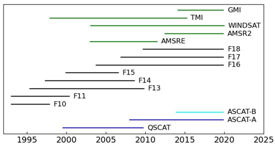
Figure 1.
Times that each satellite contributes to CCMP. Scatterometers are shown in blue, and radiometers are shown in black (SSM/I series,) and green. Those shown in green include the lower frequency 11 GHz channel. ASCAT-B is shown in light blue because it is withheld from CCMP and is instead used as a source of validation winds.
2.2. NWP Winds from ERA5
In our investigation, we choose to use a background wind field from the ERA5 reanalysis [12]. We made this choice for several reasons: (1) ERA5 is available at high spatial resolution (0.25 degrees, regridded from a native grid of ~0.31 degrees) for the entire period of interest (1993 onwards). (2) ERA5 provides 10-m equivalent neutral stability wind, which is more closely aligned with the winds measured by satellite instruments. (3) ERA5 is available as hourly maps, which will facilitate future production of CCMP winds at an interval shorter than the current six-hourly intervals. In the sections below, we describe several empirical adjustments we make to the ERA5 winds to make them agree better with scatterometers winds. Other approaches are possible, including those based on machine learning, e.g., [21,22].
2.2.1. Wind Speed Adjustments to ERA5
Because ERA5 winds are Earth-relative winds and satellite wind retrievals are relative to the moving ocean surface, we adjust the ERA5 surface winds using the surface current dataset from Ocean Surface Current Analysis Real-time (OSCAR) [23] so that the adjusted ERA5 winds are relative to the moving ocean surface to the extent of the fidelity of the OSCAR product. This adjustment likely contains substantial errors because the OSCAR currents are designed to be representative of the velocity of the uppermost 30 m of the ocean, as opposed to being at the surface. Moreover, OSCAR has uncertainties associated with the sampling of the input satellite data and the assumptions related to the use of the geostrophic and Ekman theories. Despite these error sources, the correction tends to reduce ERA5/satellite differences in regions with large current velocities such as the tropical Pacific and thus is of value. We will refer to this current-adjusted ERA5 winds as ERA5_OSCAR.
A comparison of one month of ERA5_OSCAR and scatterometer winds (Figure 2) shows that ERA5_OSCAR wind speeds are systematically lower than scatterometers for wind speed above about 17 m/s. We used a histogram matching technique to find a multiplicative adjustment to the ERA5 winds to force the two types of winds to have the same wind speed histograms. The advantage of a multiplicative adjustment is that it allows an adjustment derived from wind speed differences to be easily applied to wind vectors. Figure 3a shows the adjustment factor as a function of ERA5 wind speed for an example month, and Figure 3b,c show the speed histograms for ASCAT-A, and ERA5 before and after the adjustments were applied.
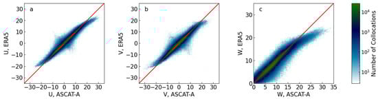
Figure 2.
2-D histograms of zonal wind (U) (a), meridional wind (V) (b) and wind speed (W) (c) for current-correct ERA5 and ASCAT-A for an example month, January 2015. Above about 17 m/s, ERA5 wind speed are systematically lower than ASCAT-A wind speed. A very similar pattern is seen in the vector components, motivating the use of a multiplicative adjustment. Note that the color scale is logarithmic to make areas with relatively low number of collocations easy to see at the expense of making the overall scatter away from the diagonal appear wider. The features in (a,b) roughly perpendicular to the diagonal do not contain many collocations. These are likely caused by relatively rare, incorrect selections for the correct “ambiguity” in the wind direction in the scatterometer retrieval.
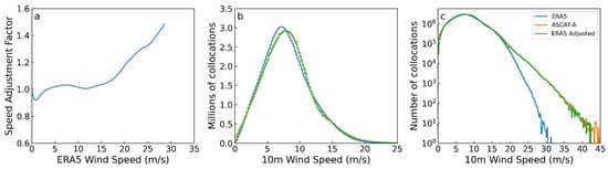
Figure 3.
(a) Multiplicative wind speed adjustment factor derived by analyzing ERA5/ASCAT-A collocations for 2015. (b) Global histograms of the 10 m equivalent neutral wind speed for ERA5, ASCAT-A, and ERA5 Adjusted accumulated over 2015. (c) Same as (b), except plotted on a log scale. In this example, we derive a global correction for all months. The correction is fairly small at low and moderate wind speeds, but begins to increase rapidly above about 17 m/s. When the correction is applied to the unadjusted ERA5 winds (blue in panels b and c), the resulting histogram (green in panels b and c), is almost indistinguishable from the ASCAT-A histogram (orange in panels b and c) for the same period, demonstrating the success of the method.
Further investigation reveals that the derived adjustment is not constant with location or time of year. We found that when the adjustment is allowed to vary with wind speed, latitude and time of the year, these differences were more accurately removed. We derive a multiplicative adjustment for each 1-degree zonal band for a given month by considering collocations that are within:
- (i).
- A 7 degree-wide zonal band, extending 3 degrees on either side of the target band;
- (ii).
- The target month, as well the two months immediately before and after the target month.
Results from the entire missions of QuikSCAT, and ASCAT-A are averaged together to produce a single adjustment that depends on latitude, time of year, and wind speed. When the adjustment is applied to a given day’s ERA5 winds, these monthly adjustments are linearly interpolated to the day of the year under consideration.
The effect of these procedures is to ensure that the adjustment is smoothly varying in both time and latitude. Because the adjustment does not depend on the year being adjusted, the effect on the long-term changes in ERA5 winds is only of second order, with the main long-term effect being the amplification of year-to-year variations at high wind. Figure 4 shows the multiplicative adjustment applied as a color-coded image for two example months. At all latitudes and for both example months, the correction is fairly small below ~17 m/s, and then grows at higher wind speeds. The main difference between the different months is the region of low (<1.0) correction values at low wind speed in the hemisphere experiencing summer. This may be due to regional errors in the atmospheric stability. Maps of the difference between ERA5 and scatterometer wind speed consistently show regions of large positive differences to the east of large continents in the summer season similar to those shown in [5] for CCMP 1.0 and the ECWWF analysis. These regions often exhibit high stability because of the advection of warm continental air over the cooler ocean. The high stability reduces the mixing of winds aloft mixing down to the ocean surface. The opposite is seen in the winter season, when cold continental air in these locations can advect over the relatively warm ocean, leading to low stability and efficient vertical mixing.
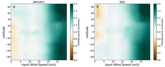
Figure 4.
Color-coded representations of the wind speed adjustment factor applied to ERA5 winds as a function of ERA5 wind speed and latitude. We show the adjustments for two example months, January (a) and July (b). Adjustments for all other months are qualitatively similar, except for the seasonal variation of the low-speed corrections described in the text.
2.2.2. Wind Vector Adjustments to ERA5
After the wind speed adjustments are applied, some regional differences in the vector components remain. The spatial patterns of these differences suggest that they are at least partly related to stability conditions, as large values occur over the Inter-Tropical Convergence Zone (ITCZ) and areas of persistent currents that cause perturbations in the sea surface temperature. They may also be related to errors in the adjustment made for ocean currents. Since these differences are fairly constant from year to year and are similar for QuikSCAT and ASCAT-A, but with substantial seasonal variations, we remove them by subtracting a spatially smoothed, seasonally varying mean ERA5-scatterometer difference, averaged over both the QuikSCAT and ASCAT-A missions. The smoothing is performed by fitting the differences to a series of spherical harmonics Ylm, with l extending from 0 to lmax = 40. We choose this value of lmax so that the smoothed version largely preserves the sharp feature near the ITCZ in the tropical Pacific, but removes most of the noise on shorter (<~5 degrees) distance scales. An example of the regional adjustment for meridional wind over the month of June is shown in Figure 5. The adjustments applied for both zonal and meridional winds for each month of the year are shown in Figure A1 and Figure A2 in Appendix A.
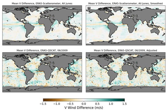
Figure 5.
Example of the construction procedure for removing vector component biases. (a) Monthly averaged meridional wind difference for June, averaged over QuikSCAT (2000–2009) and ASCAT-A (2007–2019). (b) A smoothed version of the differences in (a), obtained by fitting the data in (a) to a series of spherical harmonics Ylm, with l extending up to 40 and m to +/− 40. (c) Differences for (ERA5-QuikSCAT) meridional wind component, before adjustments are applied for June 2009. (d) Same as (c), except after the adjustment shown in (b) is subtracted. The adjustment removes much of the regional biases, particularly near the Equator.
After applying these corrections, we revisit 2-D histograms similar to those in Figure 2, except averaged over the entire 2013–2019 overlap periods of ASCAT-B and ERA5. These are plotted for the unadjusted ERA5 winds versus ASCAT-A in Figure 6a–c. The adjusted ERA5 winds are plotted as a function of ASCAT-A in Figure 6d–f and as a function of ASCAT-B in Figure 6g–i. These plots demonstrate that the wind speed correction removed the wind bias in ERA5 at high wind speeds both when evaluated using ASCAT-A winds (which were used, in combination with QuikSCAT, for the derivation of the correction) and ASCAT-B winds (which were not used to derive the correction). The similarity for the results for ASCAT-A and ASCAT-B suggests that the ERA5/ASCAT-A differences are not idiosyncratic to ASCAT-A, but instead are a persistent property of ERA5. This gives us confidence in applying the same adjustments to ERA5 winds during the period before scatterometer measurements (1993-mid 1999), though we note that the difference between ERA5 and the scatterometers may evolve over time as the amount and type of data assimilated by ERA5 changes.
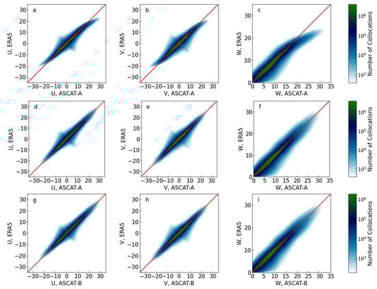
Figure 6.
Two-dimensional histograms of ERA5 winds as a function of scatterometer winds. The top row (a–c) shows the results using unadjusted ERA5 neutral stability winds and ASCAT-A winds. The second row (d–f) shows the results for ERA5 and ASCAT-A winds after the adjustment for ocean currents, speed adjustments and vector components were applied. The bottom row (g–i) is similar to the middle row, except for collocations with ASCAT-B winds were used. Note that ASCAT-B results were not used to derive any of the adjustments, confirming that the adjustments applied to ERA5 are not idiosyncratic differences arising from features of a single instrument.
As a further validation of the adjustment, we display Hovmöller diagrams of the ERA5—QuikSCAT differences in Figure 7. In this figure, each row shows the results after different adjustments steps, and each column shows a different wind variable (zonal wind, meridional wind, and wind speed). After only the ocean current corrections, there are large seasonal variations in the wind differences, particularly apparent in wind speed in the northern extratropics, and in meridional wind near the equator. After applying the wind speed correction, these differences are greatly reduced, but there is an increase in the seasonally constant zonal wind bias in the tropics. This and other small differences in the wind vector components are removed by the final regional vector wind adjustments. The final adjustment causes a small increase in the absolute wind speed differences, particularly in the QuikSCAT—ASCAT-A overlap period after 2008. A set of plots of ERA5—ASCAT-A (Figure A3) differences show similar results.
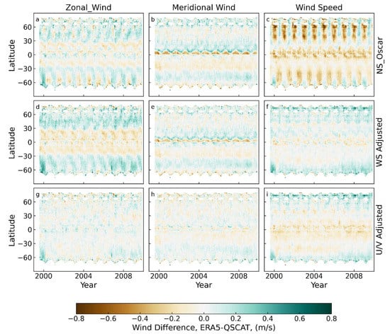
Figure 7.
Hovmöller diagrams of ERA5—QuikSCAT wind differences for 2000–2009. Panels (a–c) show the differences for zonal wind, meridional wind, and wind speed when only the ocean adjustments for currents are applied to ERA5. Panels (d–f) show the same differences after the wind speed adjustment was applied. Panels (g–i) shown the final results after the regional vector-component biases are also removed. Results for ERA5—ASCAT-A are similar (see Figure A3).
Taken together, these three figures (Figure 6, Figure 7 and Figure A3) demonstrate that our adjustment procedure is successful in greatly reducing the average differences between ERA5 winds and scatterometer winds. We note that the adjustments are not perfect. This is most apparent for the wind speed Hovmöller plots after the vector component adjustments. In comparison with both QuikSCAT and ASCAT-A, ERA5 is biased slightly low in the tropics, while in the higher southern latitudes ERA5 is biased in opposite directions relative to QuikSCAT and ASCAT-A. While these remaining small differences could likely be reduced using a more detailed adjustment procedure, the effect on the final CCMP product will be fairly small and, in our judgement, not worth the extra complication. These adjusted ERA5 (ERA5_ADJ) winds are used for the subsequent analysis in this paper.
2.3. Adjustments to Radiometer Wind
We next compare ERA_ADJ winds to winds retrieved from imaging radiometers. Radiometer measurements are important for extending CCMP to the pre-scatterometer period. For this analysis, we separate the radiometer instruments into two sets, one (Rad_LO) that includes instruments that have a lower 11 GHz channel (TMI, AMSR-E, AMSR2, WindSat and GMI) and a second set (Rad_MED) consisting of instruments whose lowest frequency channel is 19 GHz (SSM/I and SSMIS). Winds from the Rad_LO instruments are less affected by atmospheric conditions because of the increased atmospheric transparency at lower frequencies [24]. Global maps of the mean ERA5-SSM/I F13 differences are shown in Figure 8. Panels (a) and (b) show the differences for the ERA5_OSCAR and ERA5_ADJ winds. In both cases, there are large regional differences, with a small improvement when ERA5_ADJ winds are used in place of ERA5_OSCAR. We note that the overall statistical consistency between ERA5_ADJ and SSM/I F13 is good as indicated by wind speed histograms and mean differences binned by wind (not shown). Hovmöller diagrams (Figure 9) show that the differences are also strongly modulated by the seasonal cycle in regions more than about 25 degrees away from the Equator. Similar plots are shown for AMSR-E, a Rad_LO instruments, in Figure A4 and Figure A5 in the Appendix A. In both cases, the differences are large enough to make it advantageous to adjust the radiometer winds before including them in CCMP. To do this, we adjust both the Rad_LO and Rad_MED withs so they agree with the adjusted ERA5 winds. We calculated monthly mean differences between each type of radiometer and adjusted ERA5 winds by averaging over the complete missions of each set of radiometers. Only AMSR-E, AMSR2 and WindSat were included in the calculation of the Rad_LO means because TMI and GMI do not sample all latitudes due to their more inclined orbits. All Rad_MED instruments were included in the Rad_MED averages. The monthly mean adjustments for each month and radiometer type are shown in Figure A6 and Figure A7. Similar to the adjustments made to ERA5, the adjustments made to the radiometers are performed by interpolating the monthly maps to the day being adjusted. Panels (c) in Figure 8, Figure 9, Figure A4 and Figure A5 show the differences after the adjustments were applied.
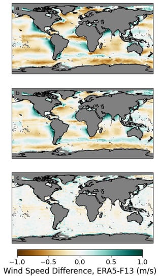
Figure 8.
Global maps of the differences between ERA5 and SSM/I F13, averaged over 1996–2009. (a) shows the differences relative to ERA5_OSCAR. There are large regional biases, with several areas showing average differences as large as 1 m/s. (b) shows the differences relative to ERA5_ADJ. The adjustments applied to ERA5 reduced the ERA5-F13 differences, but substantial regional differences remain. After regional wind speed adjustments were applied to the F13 winds, the differences are much reduced (panel c). We note that the corrections applied to F13 was derived using all Rad_MED instruments (F10, F11, F13, F14, F15, F16, F17 and F18). The success of these adjustment for F13 indicates that the differences are consistent across instruments of the same type.
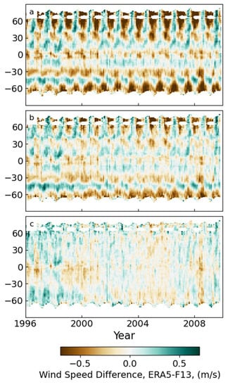
Figure 9.
Hovmöller diagrams of the differences between ERA5 and SSM/I F13. (a) shows the differences relative to ERA5_OSCAR. There are large seasonally modulated differences poleward of about 25°S and 25°N. (b) shows the differences relative to ERA5_ADJ. The adjustments applied to ERA5 reduced the ERA5-F13 seasonal differences. After wind speed adjustments were applied to the F13 winds, the seasonal differences are much reduced (c). The remaining differences are mostly lower than 0.2 m/s and do not show a consistent seasonal pattern.
2.4. CCMP Processing
The CCMP analysis combines surface wind observations from satellites with a background field derived from operation analyses or reanalysis to produce a gap-free near-global oceanic vector wind map every 6 h. Each map is calculated using a variational approach [5]. The method fills in the gaps between satellite swaths and adds direction information to satellite measurements of scalar wind speed. The resulting gridded map corresponds an estimate of the wind field at a single synoptic time instead of the range of times represented in a satellite dataset. These features make the dataset much easier to use than the raw satellite data in a variety of oceanographic and meteorological applications. The variational analysis method (VAM) is constructed so that CCMP wind speeds directly reflect observations close to the analysis time and smoothly merges these data-rich areas into the background when no close observations are available. In most cases, CCMP winds are closer to the actual satellite wind measurements than the background analyses, even though the background analysis also assimilates satellite retrievals. This difference is presumably because the analysis also assimilates a multitude of other measurements (e.g., pressure, temperature) that affect the analyzed state of the surface winds.
The CCMP VAM functions by minimizing a cost function J [5],
Here, A, B, and O denote analysis, background and observations. V is a wind vector with components u, v. are the stream function, vorticity and relative vorticity. The first two terms in the cost function reflect the contribution to the misfit of the analysis from the different types of satellite observations, where: SCAT = satellite scatterometer, and SPD = satellite wind speed (from scatterometers and radiometers). The remaining terms control the magnitude and smoothness of the difference between the analysis and the background (VWM = vector wind magnitude), a priori smoothing constraints (LAP = Laplacian of wind components, DIV = divergence, and VOR = vorticity), and a dynamic constraint (DYN) that limits the time rate of change of the wind field. The CCMP analysis was constructed using a multistage procedure that allows for both adaptive quality control and analysis at a cascade of increasingly finer length scales for computational efficiency. The λ’s are weights that control the influence each type of constraint has on the final results. The values of the λ’s were chosen in previous work [5] using a sensitivity analysis, with several goals. First, the output of the analysis should be close to satellite measurements in regions where satellite observations closely collocated in time are available. Second, fine features at the 1/4-degree scale present in the satellite data should be largely preserved. Third, the wind fields should smoothly transition to the adjusted background field in the boundaries between regions with and without satellite observations. In large regions without satellite observations, CCMP is very close to the background field. The weights were chosen so that the root mean square (RMS) difference between vector components of closely coeval satellite observations and the CCMP analysis is about 0.5 to 0.7 m/s, roughly half of the typical RMS difference between satellite observations and the adjusted ERA5 winds. By increasing the satellite weights further would decrease the RMS further, but it was found in previous work [5] that this led to discontinuities near the edges of satellite swaths, particularly in regions where there were data from multiple satellites.
Satellite observations are included in the analysis if they are within 6 h of the analysis time, but the weights are reduced as the time difference increases using parabolic function [5] that reduces the weight by 50% for a time difference of 3 h and the weight is reduced to zero at a difference 6 h. If multiple data sources are available within this window, they all contribute to the final analyzed wind field. The evolution of the wind field during the analysis window is taken into account by analyzing the difference between the observations and the analysis at the observation time using time-interpolated version of the analysis. The difference is then applied at the synoptic time. This “First Guess at Appropriate Time” method implicitly assumes that the observation—analysis time is constant (probably not exactly true) but allows translation of satellite information over the relatively short time difference to the synoptic time.
To help understand the final analysis, we imagine regions with differing data availability. Far from any available satellite data, the analysis is very close to the background field, ERA5_ADJ. As we approach a region with satellite data, the analyzed field smoothly transitions to be in better agreement with the satellite data, constrained by the various smoothness constraints. When scatterometer data is available, the analyzed wind direction is influenced by both the scatterometer data, and by the background field. The smoothness constraints help limit errors in ambiguity selection from affecting the final analysis. In regions with only radiometer wind speeds, the analyzed wind speed is close to the satellite values, while the direction is largely given by the background field, but still subject to the smoothness constraints. The CCMP method is described in considerable detail in [5] and more recent results from the Near-Real-Time (NRT) version of CCMP are presented in [8]. For the work described here, we have performed the CCMP analysis for the time period from January, 1993 (the advent of the OSCAR current dataset and thus the possibility of adjusting ERA5 winds for currents) to December 2019.
For the purpose of this study, we withhold retrievals from ASCAT-B from the CCMP processing. Withholding this data source will allow us to use ASCAT-B as independent datasets to evaluate the accuracy and stability of CCMP. In the remainder of the manuscript, we will refer to the resulting CCMP version as CCMP ADJ, to remind the reader that this new version adjusted values for the background field and radiometer winds as the input. When the new version is released to the public on the RSS website, it will be called CCMP 3.0. A table summarizing the names and properties of the various non-satellites input and output datasets is shown in Table 2.
Table 2.
Non-satellite datasets used or discussed in the manuscript.
3. Results
3.1. Comparison versus ASCAT-B
In this section, we present comparisons between CCMP and ASCAT-B. ASCAT-B is a C-Band scatterometer operated by EUMETSAT, mounted on the MetOp-B platform. It began operation in late 2012 and operated continuously until the present time (mid 2022), covering the remainder of the CCMP ADJ period (1993–2019). For this study, we will consider wind retrievals produced by RSS from 2013–2019. These winds are well-calibrated to both ASCAT-A and to wind speeds from imaging radiometers and verified versus global moored buoy observations [15].
As we noted above, ASCAT-B was not used to construct the pre-merge adjustments wind applied to ERA5 or radiometer winds, or used to produce CCMP ADJ. Comparing to other satellites that were included in CCMP ADJ is not useful for assessing the accuracy of the CCMP, because the variational analysis strongly “pulls” the CCMP output to the satellite winds. Because of this, any comparison with the included satellite winds would suggest uncertainty and bias in CCMP that is considerably lower than the actual uncertainty in the CCMP product. For the results presented here, we only use ASCAT-B observations that occur within 1 h of the 6-hourly CCMP analysis times. For ASCAT-B, which has a nearly constant local Equator crossing time (9:30 am/pm), this has the effect of limiting the longitudes sampled in the comparison.
When doing the comparison between CCMP and ASCAT-B, we separate the CCMP winds into two subsets, those at all collocations (denoted by ALL), and those without a closely collocated satellite (denoted by NOSAT). The ALL collocations provide an overall picture of the quality of CCMP, while the NOSAT focuses on results that are mostly influenced by the background winds. In previous versions of CCMP, the NOSAT locations were biased low compared to locations with satellite observations. NOSAT locations can occur either because the location is in a gap between all the included satellites observations, or because the data from satellites were excluded because of rain contamination. In Figure 10, we show a typical map of locations where CCMP is collocated with ascending ASCAT-B over a day, color-coded by SAT and NOSAT observations. The map shows that most of the time, there is a nearby satellite observation for CCMP. Most of the NOSAT locations on this day occur because of rain flagging in the CCMP-ingested satellites except for the triangular regions missing from some swaths in the Southern Ocean.
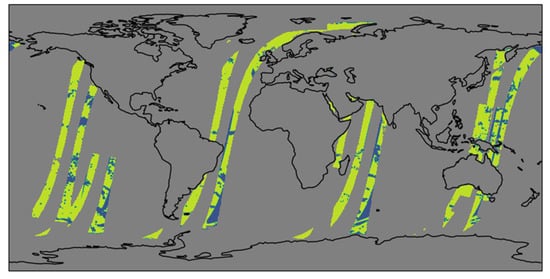
Figure 10.
Map of collocations between ASCAT-B and CCMP for an example day (1 January 2018), for the ascending passes of ASCAT-B. Locations where CCMP included a satellite observation from any satellite (SAT) are shown in yellow and locations without a satellite in CCMP (NOSAT) are shown in blue. NOSAT collocations occur for two reasons: (1) Satellite observations were excluded from CCMP because of rain contamination. These are the irregularly shaped regions spread across the map. (2) The existence of gaps between satellite swaths even when all satellites are included. For this day/node, this only occurs in the Southern Ocean and on the extreme left side of a few swaths near the equator. The locations of the satellite gaps vary over time as the swaths for the other satellites drift with respect to ASCAT-B.
We also compare winds from 3 versions of CCMP and the adjusted version of the ERA5 background field (ERA5 ADJ). The CCMP versions are (1) CCMP 2.0, (2) CCMP NRT as described in [8] which uses the NCEP GFS 0.25 analysis as the background, and (3) CCMP ADJ.
3.1.1. Maps of Mean and RMS Difference
In Figure 11 and Figure 12, we show maps of the mean and RMS difference between CCMP ADJ and ASCAT-B. The gaps in the map are locations where the collocations between CCMP ADJ and ASCAT-B are always separated by more than 1 h. The absolute mean differences (Figure 11) are almost always less than 0.5 m/s, except for a few locations in the Southern Ocean. The largest of these occur near the edge of the missing regions where the collocations may be degraded by excess time difference, which can be important for fast-moving mid-latitude storms, or sampling effects.
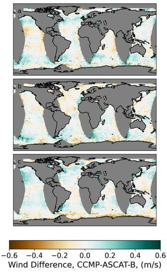
Figure 11.
Maps (a), Zonal Wind; (b), Meridional Wind; (c)-Wind Speed of mean difference between CCMP ERA5 ADJ. vs. ASCAT-B, averaged over the 2013–2019 period. These maps were made using all rain-free ASCAT-B collocations and are intended to serve as an estimate of the performance of the CCMP ERA5 ADJ wind product.
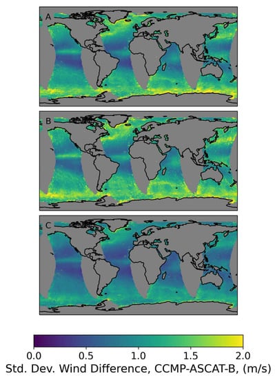
Figure 12.
Maps (A), Zonal Wind; (B), Meridional Wind; (C), Wind Speed of standard deviation of the difference between CCMP ERA5 ADJ. vs. ASCAT-B, averaged over the 2013–2019 period. As was the case for Figure 11 these maps were made using all rain-free collocations and are intended to serve as an estimate of the performance of the CCMP ERA5 ADJ wind product.
The standard deviation of the differences varies considerably with location. The smallest standard deviation of the differences are in the subtropical oceans, where the winds are of moderate strength and show less spatial variability than other regions. Closer to the equator, the standard deviation of the differences is larger (Figure 12). This is likely a combination of several factors, including the partial absence of satellite observations in CCMP due to rain contamination, undetected rain in the ASCAT-B observations, and wind direction ambiguity selection error in the ASCAT-B retrievals, which are most likely to occur at low wind speeds which are common in the tropics.
The standard deviation of the differences is also relatively larger in the mid and sub-polar latitudes, where rapidly moving extratropical cyclones increase the effects of the time differences between observations and CCMP (which itself is constructed from observations over a 6-h time span). The higher wind speeds in these regions also amplify direction errors when the winds are expressed as vector components. Note that the standard deviations of the differences for both U and V are larger than those for wind speed in the high latitudes, indicating that direction errors are the dominant contributor to errors in vector components.
3.1.2. Hovmöller Plots
Maps such as those shown in Figure 11 and Figure 12 do not provide any information on the time dependence of the ASCAT-B-CCMP differences. To investigate the time dependence, in Figure 13 we show Hovmöller diagrams of the difference between ASCAT-B winds and three versions of CCMP, as well as ocean-current-adjusted (but not speed adjusted) version of ERA5. Differences with ERA5 (panels j–l) show large seasonal differences in wind speed poleward of 30 N and 30 S. Part of these differences are caused by the negative bias in ERA5 at higher wind speeds more common in each hemisphere’s winter months. Differences with CCMP 2.0 (g–i) show latitude-dependent biases in zonal wind and wind speed, as well as a decreasing relative trend in CCMP 2.0. Differences with CCMP NRT (d–f) (which begins in January 2015) also show latitude dependent biases, particularly in zonal wind. CCMP ADJ (a–c) shows smaller differences than any of the previous versions or ERA5, though there is still a small increasing trend in CCMP ADJ wind speed differences at most latitudes, perhaps caused by small trends in radiometer wind retrievals relative to ASCAT-B.
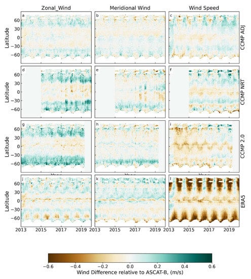
Figure 13.
Hovmöller plots of CCMP-ASCAT-B differences for 3 versions of CCMP and ERA5-Oscar. Note that CCMP NRT begins in early 2015, and CCMP 2.0 ends before the end of 2019. (a–c) zonal wind, meridional wind and wind speed differecnes for CCMP ADJ—ASCAT-B. (d–f) same as (a–c) except for CCMPT-NRT—ASCAT-B. (g–i) same as (a–c), except for CCMP 2.0—ASCAT-B. (j–l) same as (a–c), except for ERA-5—ASCAT-B.
3.1.3. Histograms
In Figure 14, we show histograms of wind speed for collocated ASCAT-B and the same set of CCMP and ERA5 winds used above. For CCMP, we show histograms for the NOSAT case (a and c). ERA5 winds are shown on the same plot as the ALL CCMP cases (b and d). The panels in the bottom row (c and d) are plotted on a linear-log scale to emphasize the results at the tail of the distribution at high winds. In both collocation subsets, these plots demonstrate that the adjustment to the ERA5 background field has achieved one of our goals for CCMP ADJ: CCMP wind speed histograms now closely match the histograms from ASCAT-B for both the NOSAT and ALL collocations subsets.
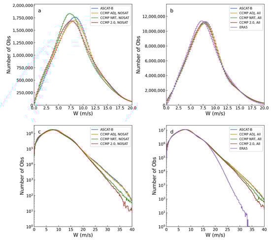
Figure 14.
Histograms of wind speed for ASCAT-B, three version of CCMP and ERA5. Panels (a) and (c) show the results for collocations without satellite observations in CCMP, and (b,d) show all colocations. Panels (a–d) are identical except for the vertical axis, which is displayed in logarithmic form in (c,d).
3.1.4. Binned Differences
Figure 15 shows mean and RMS differences for wind speed, zonal and meridional winds binned by the average wind. In wind speed (a and b), the results confirm that ERA5 is biased low at wind speeds above ~15 m/s. Earlier versions of CCMP (2.0 and NRT) are also biased low at wind speeds above ~20 m/s, mostly due to large biases for the NOSAT subset of collocations. CCMP ADJ shows little systematic bias over the entire range for both the NOSAT and ALL subsets. The RMS differences are also lowest for CCMP ADJ. Similar results for zonal (c and d) and meridional (e and f) are plotted in the rest of the panels. The U and V are not completely unbiased at high wind but the biases are much reduced. The residual bias in both U and V is likely due to the effects of direction error. The RMS error is also reduced in CCMP ADJ relative to the earlier versions. Summary statistics averaged over all wind speeds are shown in Table 3, and statistics average over high winds (wind speed > 15 m/s) are shown in Table 4.
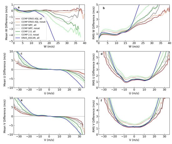
Figure 15.
Binned mean differences and RMS differences between wind and ASCAT-B. The left column (a,c,e) shows the mean differences for W, U, and V as a function the average wind between the wind variable pairs. The right column (b,d,f) shows the RMS differences. In all cases, CCMP ERA5 ADJ shows better agreement with ASCAT-B than the other wind datasets.
Table 3.
Mean and RMS of Wind differences vs. ASCAT-B over all wind speeds.
Table 4.
Mean and RMS of Wind differences vs. ASCAT-B over all wind speeds > 15 m/s.
3.2. Long-Term Trends
In this section, we briefly evaluate the long-term trends in CCMP, the ERA5 background field, and a multi-satellite merged wind speed dataset constructed using wind speed from RSS radiometers. Part of the motivation for making the pre-merge adjustments to the ERA5 background field and the radiometer data is to prevent systematic differences between wind sources from being aliased into long-term trends as the number of satellite observations varies over time. Figure 16 shows the annual mean, near globally averaged (60S–60N) time series for various sources of ocean winds. All datasets show increasing wind speed from 1993 until 1998, a sharp dip in 2009, and then a slow decline after 2010. The overall trend for CCMP 2.0 (0.0514 m/s per decade) is larger than for the other three datasets, which range from 0.0052 to 0.0294 m/s per decade. The larger trend in CCMP 2.0 is largely caused by the large trend from 1993–2003, the period over which the number of satellite observations is increasing. In contrast, CCMP ADJ shows similar trends to ERA5 and RSS radiometers over this period, indicating that the pre-merge adjustments were successful in removing spurious trends.
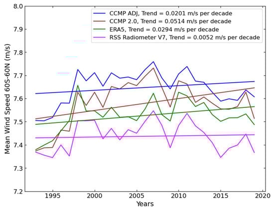
Figure 16.
Time series of annual, globally averaged (60S–60N) mean wind speed for two versions of CCMP, ERA5_OSCAR, and merged RSS radiometer winds.
The four datasets also differ in overall average wind. The larger mean wind for CCMP ADJ relative to ERA5 is not surprising, because the ERA5 winds above ~17 m/s were increased before ingestion by CCMP ADJ. The larger winds in CCMP ADJ than in RSS radiometers is likely due to missing data caused by rain in the radiometer data. In most areas of the ocean, rain is accompanied by higher-than-average wind speeds. When parts of the high wind regions are missing because of rain contamination, the overall average winds are lowered. Figure 17 shows maps of wind speed trends (1993–2019) for the four datasets. There is excellent agreement between CCMP ADJ and ERA5 and RSS Radiometers. CCMP 2.0 shows larger overall trends than the other datasets, as well as more variability with location.
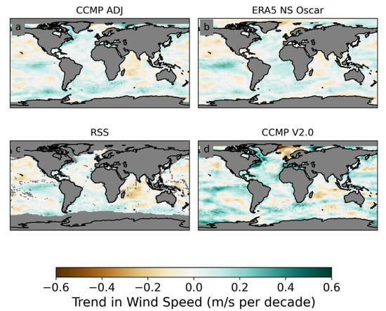
Figure 17.
Maps of Trends in wind speed (1993–2019) for two versions of CCMP (a,d), ERA5 NS Oscar (b), and RSS radiometer winds (c). CCMP ADJ is in much better agreement with ERA5 and with the radiometer winds than CCMP 2.0.
4. Discussion
By adjusting the ERA5 background field and radiometer winds before using these data sources in the CCMP variational analysis, we have produced a version of CCMP ADJ that is more consistent with scatterometer winds, particularly at high wind speed. By withholding data from the ASCAT-B scatterometer from the CCMP analysis, we show that the CCMP ADJ is consistent with ASCAT winds for 2013–2019. Comparisons with ASCAT-B also allows us to estimate the uncertainty in CCMP wind speed and vector components as a function of wind speed. The results of this analysis show that the new version is an improvement over previous versions of CCMP as well as over the ERA5 background field, particularly at winds > 15 m/s. We note that because ASCAT-A and ASCAT-B winds are retrieved using the same algorithm, there may be common systematic biases in CCMP ADJ and ASCAT-B that would not be discovered in this study.
We note that these results only strictly apply for the 2013–2019 period where we made comparison with ASCAT-B. We are moderately confident that the results are representative of the scatterometer era, beginning with the launch of QuikSCAT in mid-1999. The differences between ERA5 and scatterometer winds are stable over this period, suggesting that the adjustments we made to the background field are appropriate and necessary. Before the launch of QuikSCAT, the adjustments are less well supported. It is possible that the distribution of the ERA5 winds for 1993–1999 differs from the distribution for the later period because no satellite vectors winds were available for ERA5 to assimilate. This would mean that the adjustments we made to ERA5 winds pre-1999 (which are based on comparisons with scatterometer winds after 1999) are not ideal. Determining if this is a problem or not is difficult. The effect of the adjustments is only large for wind speeds above 15 m/s. Errors in these high winds cannot be determined unambiguously by comparisons with in situ winds, which are both uncommon at high winds, and potentially biased or unreliable [25,26]. Despite these limitations, we have concluded that is appropriate to adjust the pre-QuikSCAT ERA5 winds because we suspect that an important contribution to the ERA5 low bias at high winds is due to limitations to the ERA5 model in resolving short-length-scale features where most of the high winds occur. We caution that small, intense features such as tropical cyclones are not well represented in ERA5 because of the 0.31-degree native resolution in ERA5. Since many satellite wind retrievals are missing in tropical cyclone because of rain, these features are not well represented in any version of CCMP. Therefore, CCMP should not be used to study tropical cyclones though it may be useful to investigate cyclogenesis. Further validation of this new version of the CCMP winds using independent buoy wind measurements is underway. The results will be reported in subsequent manuscripts and will indicate how well short time scale phenomena, such as westerly wind bursts or diurnal variation, are represented in CCMP 3.0.
Author Contributions
Conceptualization, T.L., C.M. and F.W.; methodology, C.M. and T.L.; software, C.M.; validation, C.M.; formal analysis, C.M. and T.L.; investigation, C.M.; resources, F.W. and T.L.; data curation, C.M., L.R., F.W. and X.W.; writing—original draft preparation, C.M.; writing—review and editing, C.M., T.L. and L.R.; visualization, C.M.; supervision, C.M. and T.L.; project administration, T.L.; funding acquisition, T.L. All authors have read and agreed to the published version of the manuscript.
Funding
This research was funded by NASA Physical Oceanography Program. Part of the research was carried out at the Jet Propulsion Laboratory, California Institute of Technology, under a contract with the National Aeronautics and Space Administration (80NM0018D0004).
Data Availability Statement
Satellite-derived input data used in this study are available from Remote Sensing Systems (www.remss.com, accessed on 15 June 2021). The ERA5 background fields [12] were downloaded from the Copernicus Climate Change Service (C3S) Climate Data Store (https://cds.climate.copernicus.eu/ accessed on 15 June 2021). The data for 1993–2018 were downloaded in March 2019. The date for 2019 was downloaded in January 2020. The results contain modified Copernicus Climate Change Service information 2020. Neither the European Commission nor ECMWF is responsible for any use that may be made of the Copernicus information or data it contains. The OSCAR surface current product [25] was downloaded in February 202 from the Physical Oceanography Distributed Active Archive Center (PO.DAAC) https://podaac.jpl.nasa.gov/dataset/OSCAR_L4_OC_third-deg accessed on 15 June 2021. The CCMP Analysis produced using the methods described here are freely available for download (after registration) from Remote Sensing System (https://www.remss.com/measurements/ccmp/ accessed on 25 July 2022) where it is called CCMP 3.0.
Acknowledgments
The authors would like to thank the anonymous reviewers for their enriching insights and comments. The authors are also grateful for the continuous support from the NASA OVWST program, and to many members of the IOVWST group for useful discussions over the numerous Science Team meetings.
Conflicts of Interest
The authors declare no conflict of interest. The funders had no role in the design of the study; in the collection, analyses, or interpretation of data; in the writing of the manuscript, or in the decision to publish the results.
Appendix A
This appendix contains additional supporting figures referenced in the main text.
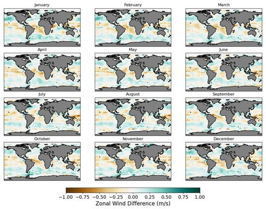
Figure A1.
Maps of monthly zonal wind adjustments applied to speed-adjusted ERA5 winds.
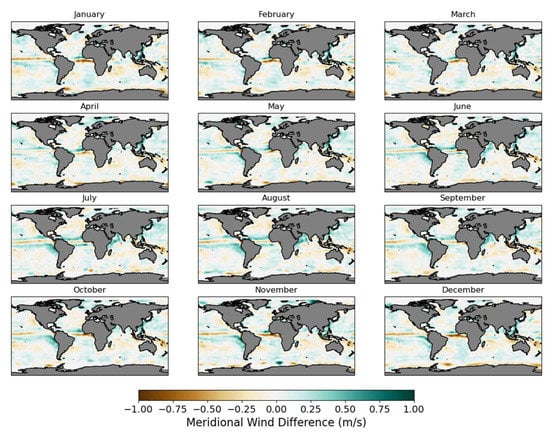
Figure A2.
Months of monthly meridional wind adjustments applied to speed-adjusted ERA5 winds.
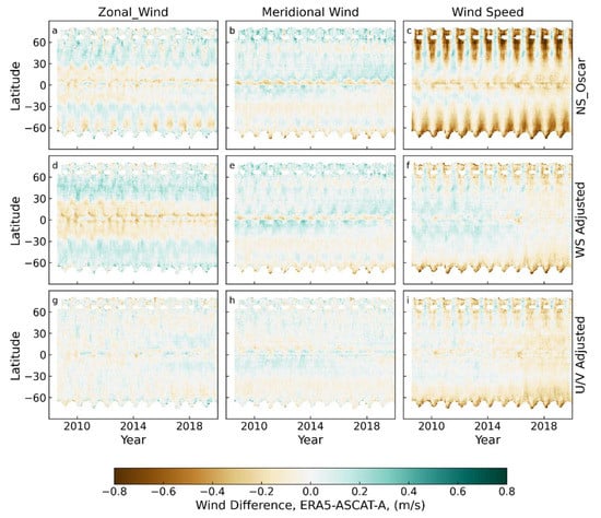
Figure A3.
Similar to Figure 7 in the main text, except for ASCAT-A. Hovmöller diagrams of ERA5—ASCAT-A wind differences for 2000–2009. Panels (a–c) show the differences for zonal wind, meridional wind, and wind speed when only the ocean current adjustments are applied to ERA5. Panels (d–f) show the same differences after the wind speed adjustment was applied. Panels (g–i) shown the final results after location-dependent vector-component biases are also removed.
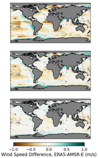
Figure A4.
Similar to Figure 8 in main text, except for AMSR-E. Global maps of the differences between ERA5 and AMSRE, averaged over 2003–2010. (a) shows the differences relative to ERA5_OSCAR. As was the case for SSM/I F13, there are large regional biases. (b) shows the differences relative to ERA5_ADJ. The adjustments applied to ERA5 reduced the ERA5-AMSR-E differences substantially, but some regional differences remain. After wind speed adjustments were applied to the AMSR-E winds, the differences are much reduced (c). We note that the corrections applied to AMSR-E we derived using all Rad_LO instruments with global coverage (AMSR-E, AMSR2, and WindSat).
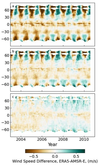
Figure A5.
Similar to Figure 9 in the main text, except for AMSR-E. Hovmöller diagrams of the differences between ERA5 and AMSR-E. (a) shows the differences relative to ERA5_OSCAR. There are large seasonally modulated differences poleward of about 25 degrees north and south. (b) shows the differences relative to ERA5_ADJ. The adjustments applied to ERA5 reduced the ERA5-AMSR-E seasonal differences. After WS adjustments were applied to the AMSR-E winds, the seasonal differences are much reduced (c). The remaining differences are mostly less than 0.25 m/s with a small trend over the period.
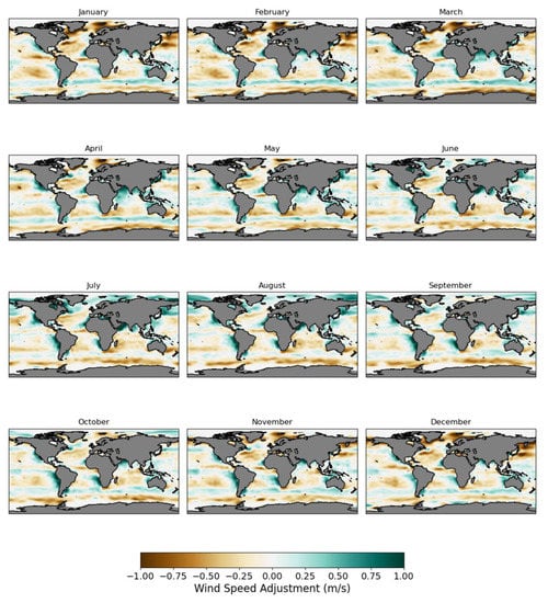
Figure A6.
Wind Speed Adjustments applied to RAD_MED radiometer winds before inclusion in CCMP.
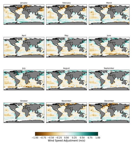
Figure A7.
Wind Speed Adjustments applied to RAD_LO winds before inclusion in CCMP.
References
- Schuster, U.; Monteiro, P.M.S.; Tilbrook, B.D.; Lenton, A.A.; Sabine, C.; Takahashi, T.; Wanninkhof, H.; Hood, M.; Watson, A.J.; Olsen, A.; et al. Remotely Sensed Winds and Wind Stresses for Marine Forecasting and Ocean Modeling. In Proceedings of the OceanObs’09: Sustained Ocean Observations and Information for Society, Venice, Italy, 31 December 2010; pp. 78–93, European Space Agency. [Google Scholar]
- Chelton, D.B.; Schlax, M.G.; Freilich, M.H.; Milliff, R.F. Satellite Measurements Reveal Persistent Small-Scale Features in Ocean Winds. Science 2004, 303, 978–983. [Google Scholar] [CrossRef]
- Wentz, F.J.; Ricciardulli, L.; Rodriguez, E.; Stiles, B.W.; Bourassa, M.A.; Long, D.G.; Hoffman, R.N.; Stoffelen, A.; Verhoef, A.; O’Neill, L.W.; et al. Evaluating and Extending the Ocean Wind Climate Data Record. IEEE J. Sel. Top. Appl. Earth Obs. Remote Sens. 2017, 10, 2165–2185. [Google Scholar] [CrossRef] [PubMed]
- Xue, Y.; Huang, B.; Hu, Z.-Z.; Kumar, A.; Wen, C.; Behringer, D.; Nadiga, S. An Assessment of Oceanic Variability in the NCEP Climate Forecast System Reanalysis. Clim. Dyn. 2011, 37, 2511–2539. [Google Scholar] [CrossRef]
- Atlas, R.M.; Hoffman, R.N.; Ardizzone, J.; Leidner, S.M.; Jusem, J.C.; Smith, D.K.; Gombos, D. A Cross-Calibrated, Multi-Platform Ocean Surface Wind Velocity Product for Meteorological and Oceanographic Applications. Bull. Am. Meteorol. Soc. 2011, 92, 157–174. [Google Scholar] [CrossRef]
- Desbiolles, F.; Bentamy, A.; Blanke, B.; Roy, C.; Mestas-Nuñez, A.M.; Grodsky, S.A.; Herbette, S.; Cambon, G.; Maes, C. Two Decades [1992–2012] of Surface Wind Analyses Based on Satellite Scatterometer Observations. J. Mar. Syst. 2017, 168, 38–56. [Google Scholar] [CrossRef]
- Yu, L.; Jin, X. Buoy Perspective of a High-Resolution Global Ocean Vector Wind Analysis Constructed from Passive Radiometers and Active Scatterometers (1987–Present). J. Geophys. Res. Ocean. 2012, 117, C11013. [Google Scholar] [CrossRef]
- Mears, C.A.; Scott, J.; Wentz, F.J.; Ricciardulli, L.; Leidner, S.M.; Hoffman, R.; Atlas, R. A Near-Real-Time Version of the Cross-Calibrated Multiplatform (CCMP) Ocean Surface Wind Velocity Data Set. J. Geophys. Res. Ocean. 2019, 124, 6997–7010. [Google Scholar] [CrossRef]
- Uppala, S.; Kållberg, P.W.; Simmons, A.J.; Andrae, U.; Da Costa Bechtold, V.; Fiorino, M.; Gibson, J.K.; Haseler, J.; Hernandez, A.; Kelly, G.A.; et al. The ERA-40 Re-Analysis. Q. J. R. Meteorol. Soc. 2005, 131, 2961–3013. [Google Scholar] [CrossRef]
- Dee, D.P.; Uppala, S.M.; Simmons, A.J.; Berrisford, P.; Poli, P.; Kobayashi, S.; Andrae, U.; Balmaseda, M.A.; Balsamo, G.; Bauer, P.; et al. The ERA-Interim Reanalysis: Configuration and Performance of the Data Assimilation System. Q. J. R. Meteorol. Soc. 2011, 137, 553–597. [Google Scholar] [CrossRef]
- McGregor, S.; Sen Gupta, A.; Dommenget, D.; Lee, T.; McPhaden, M.J.; Kessler, W.S. Factors Influencing the Skill of Synthesized Satellite Wind Products in the Tropical Pacific. J. Geophys. Res. Ocean. 2017, 122, 1072–1089. [Google Scholar] [CrossRef]
- Hersbach, H.; Bell, B.; Berrisford, P.; Hirahara, S.; Horányi, A.; Muñoz-Sabater, J.; Nicolas, J.; Peubey, C.; Radu, R.; Schepers, D.; et al. The ERA5 Global Reanalysis. Q. J. R. Meteorol. Soc. 2020, 146, 1999–2049. [Google Scholar] [CrossRef]
- Geernaert, G.; Katsaros, K.B. Incorporation of Stratification Effects on the Oceanic Roughness Length in the Derivation of the Neutral Drag Coefficient. J. Phys. Oceanogr. 1986, 16, 1580–1584. [Google Scholar] [CrossRef]
- Ricciardulli, L.; Wentz, F.J. A Scatterometer Geophysical Model Function for High Winds: QuikSCAT Ku-2011. J. Atmos. Ocean. Technol. 2015, 32, 1829–1846. [Google Scholar] [CrossRef]
- Ricciardulli, L.; Manaster, A. Intercalibration of ASCAT Scatterometer Winds from MetOp-A, -B, and -C, for a Stable Climate Data Record. Remote Sens. 2021, 13, 3678. [Google Scholar] [CrossRef]
- Manaster, A.; Ricciardulli, L.; Meissner, T. Validation of High Ocean Surface Winds from Satellites Using Oil Platform Anemometers. J. Atmos. Ocean. Technol. 2019, 36, 803–818. [Google Scholar] [CrossRef]
- Meissner, T.; Ricciardulli, L.; Wentz, F.J. Capability of the SMAP Mission to Measure Ocean Surface Winds in Storms. Bull. Am. Meteorol. Soc. 2017, 98, 1660–1677. [Google Scholar] [CrossRef]
- Mai, M.; Zhang, B.; Li, X.; Hwang, P.A.; Zhang, J.A. Application of AMSR-E and AMSR2 Low-Frequency Channel Brightness Temperature Data for Hurricane Wind Retrievals. IEEE Trans. Geosci. Remote Sens. 2016, 54, 4501–4512. [Google Scholar] [CrossRef]
- Gaiser, P.W.; St. Germain, K.M.; Twarog, E.; Poe, G.; Purdy, W.; Richardson, D.; Grossman, W.; Jones, W.L.; Spencer, D.; Golba, G.; et al. The WindSat Spaceborne Polarimetric Microwave Radiometer: Sensor Description and Early Orbit Performance. IEEE Trans. Geosci. Remote Sens. 2004, 42, 2347–2361. [Google Scholar] [CrossRef]
- Wentz, F.J. A 17-Year Climate Record of Environmental Parameters Derived from the Tropical Rainfall Measuring Mission (TRMM) Microwave Imager. J. Clim. 2015, 28, 6882–6902. [Google Scholar] [CrossRef]
- Li, Y.; Huang, W.; Lyu, X.; Liu, S.; Zhao, Z.; Ren, P. An Adversarial Learning Approach to Forecasted Wind Field Correction with an Application to Oil Spill Drift Prediction. Int. J. Appl. Earth Obs. Geoinf. 2022, 112, 102924. [Google Scholar] [CrossRef]
- Gonzalez-Arceo, A.; Zirion-Martinez de Musitu, M.; Ulazia, A.; del Rio, M.; Garcia, O. Calibration of Reanalysis Data against Wind Measurements for Energy Production Estimation of Building Integrated Savonius-Type Wind Turbine. Appl. Sci. 2020, 10, 9017. [Google Scholar] [CrossRef]
- Bonjean, F.; Lagerloef, G.S.E. Diagnostic Model and Analysis of the Surface Currents in the Tropical Pacific Ocean. J. Phys. Oceanogr. 2002, 32, 2938–2954. [Google Scholar] [CrossRef]
- Wentz, F.; Meissner, T. Atmospheric Absorption Model for Dry Air and Water Vapor at Frequencies below 100 GHz Derived from Spaceborne Radiometer Observations. Radio Sci. 2016, 51, 381–391. [Google Scholar] [CrossRef]
- Wright, E.E.; Bourassa, M.A.; Stoffelen, A.; Bidlot, J.-R. Characterizing Buoy Wind Speed Error in High Winds and Varying Sea State with ASCAT and ERA5. Remote Sens. 2021, 13, 4588. [Google Scholar] [CrossRef]
- Ricciardulli, L.; Foltz, G.R.; Manaster, A.; Meissner, T. Assessment of Saildrone Extreme Wind Measurements in Hurricane Sam Using MW Satellite Sensors. Remote Sens. 2022, 14, 2726. [Google Scholar] [CrossRef]
Publisher’s Note: MDPI stays neutral with regard to jurisdictional claims in published maps and institutional affiliations. |
© 2022 by the authors. Licensee MDPI, Basel, Switzerland. This article is an open access article distributed under the terms and conditions of the Creative Commons Attribution (CC BY) license (https://creativecommons.org/licenses/by/4.0/).