Improving Mountain Snow and Land Cover Mapping Using Very-High-Resolution (VHR) Optical Satellite Images and Random Forest Machine Learning Models

Abstract

Very-high-resolution (VHR) optical imaging satellites can offer precise, accurate, and direct measurements of snow-covered areas (SCA) with sub-meter to meter-scale resolution in regions of complex land cover and terrain. We explore the potential of Maxar WorldView-2 and WorldView-3 in-track stereo images (WV) for land and snow cover mapping at two sites in the Western U.S. with different snow regimes, topographies, vegetation, and underlying geology. We trained random forest models using combinations of multispectral bands and normalized difference indices (i.e., NDVI) to produce land cover maps for priority feature classes (snow, shaded snow, vegetation, water, and exposed ground). We then created snow-covered area products from these maps and compared them with coarser resolution satellite fractional snow-covered area (fSCA) products from Landsat (~30 m) and MODIS (~500 m). Our models generated accurate classifications, even with limited combinations of available multispectral bands. Models trained on a single image demonstrated limited model transfer, with best results found for in-region transfers. Coarser-resolution Landsat and MODSCAG fSCA products identified many more pixels as completely snow-covered (100% fSCA) than WV fSCA. However, while MODSCAG fSCA products also identified many more completely snow-free pixels (0% fSCA) than WV fSCA, Landsat fSCA products only slightly underestimated the number of completely snow-free pixels. Overall, our results demonstrate that strategic image observations with VHR satellites such as WorldView-2 and WorldView-3 can complement the existing operational snow data products to map the evolution of seasonal snow cover.

1. Introduction

As one of the most dynamic components of the cryosphere, seasonal snow is an integral part of hydrologic, ecologic, economic, cultural, and climatic systems. Snow accumulates during the cool season and releases meltwater during warmer and drier periods [1,2]. The timing and quantity of the accumulation and melt can have consequential impacts on downstream processes, phenology, and water supply [3,4,5,6], especially within mountain watersheds. Seasonal snowpack acts as a natural reservoir, providing a critical freshwater resource to over one billion people worldwide [7].

Despite the significant role of seasonal snow in many different Earth systems, understanding and measuring its distribution and water content can be challenging. Snow cover varies across a range of spatiotemporal scales based on meteorology, topography, and vegetation. Localized sources of redistribution, such as wind transport, combine with topography and vegetation processes to generate additional spatial variability after snow has fallen [8,9]. This highly heterogeneous distribution of snow suggests that in situ point measurements (e.g., snow depth from automatic weather stations) may not be representative of broader snowpack characteristics [10], especially for remote, topographically complex, and inaccessible areas. Though useful for hydrological models, the existing snow fraction estimates are insufficient for process-based ecohydrological [11,12] and ecological research that requires more fine-scale and spatially distributed information [13,14,15,16].

1.1. Satellite Snow Mapping and Mixed Pixels

Satellite remote sensing can offer measurements over large spatial extents with variable temporal coverage. Passive microwave ‘all-weather day-or-night’ approaches are capable of expansive daily coverage but with a limited spatial resolution of ~25 km and a variable performance for wet vs. dry snow. These issues limit the ability of passive microwave sensors to observe fine-scale processes affecting the highly heterogeneous snow conditions in complex terrain. Active microwave approaches (e.g., synthetic aperture radar) can offer much finer spatial resolutions (0.25–20 m), but its interpretations are affected by wet snow, vegetation, and steep topography (increased layover and shadow effects).

The widely available optical remote-sensing earth observation instruments (e.g., Moderate Resolution Imaging Spectroradiometer [MODIS] on Aqua/Terra, Enhanced Thematic Mapper Plus [ETM+] on Landsat 7, and Operational Land Imager [OLI] on Landsat 8) have been essential for mapping regional to global snow cover [17]. Snow-covered area (SCA) can be extracted from optical data using relatively simple approaches [18] given the difference in albedo between snow and other common land cover types. However, the presence of optically thick clouds and variable illumination in complex terrain still present challenges for optical remote-sensing land cover classification [19]. For a more detailed discussion of the methods and issues associated with optical remote sensing for global snow cover mapping, we refer the reader to [19,20,21,22,23].

Optical snow-cover-mapping approaches [24] routinely leverage the relatively low reflectance of snow in the shortwave infrared (SWIR) and relatively high reflectance in the visible spectrum to calculate a normalized difference snow index (NDSI), which can more effectively distinguish snow from clouds. The operational workflows to derive snow-cover products from remote-sensing satellites employ reflectance thresholding and a rule-based approach using this index for pixel-based snow classification [17,22,25]. These products are dependent on SWIR band(s) and are typically limited to a binary snow vs. “not snow” classification at the lower resolution of SWIR sensors. Thus, the spatial resolution of most publicly available snow products is relatively coarse (~15–500 m), resulting in mixed radiance values from multiple land cover features in each pixel. In one study, mixed pixels were found to comprise 25–93% of all pixels at a 40 m resolution and 67–100% at 500 m [26]. The WorldView-3 satellite can also collect SWIR image data, but the resolution is coarser than the multispectral bands (~3.7 m vs. ~1.2 m, respectively) and must be requested during tasking, with additional product costs.

Subpixel snow-mapping techniques were developed to address mixed pixels by separating snow endmembers from non-snow endmembers using field and laboratory spectral libraries [20]. These spectral unmixing models use linear spectral mixture algorithms to deconstruct constituent signals of different land-cover features. They then estimate fractional snow cover for each pixel and aggregate the fractional snow-covered area (fSCA) [21,27,28,29].

While unmixing provides estimates of the snow fraction within a pixel (with post-processing yielding values between 0–100% or 0–1), these approaches rely on well-calibrated data, both in terms of spectral libraries and radiometrically calibrated satellite instruments such as MODIS. Even with this calibration, the coarser products tend to overestimate the snow at boundaries with other feature classes [30] and are not able determine the true spatial distribution of snow at the subpixel level. To address these limitations, approaches involving downscaling, histogram matching, and data fusion techniques can potentially be used to extract finer spatial resolution fSCA products [31,32].

1.2. Very-High-Resolution Snow Mapping and Machine Learning

Despite improvements in subpixel fractional snow mapping, these techniques cannot identify small-scale snow features such as drifts or snow patches, which can be important for late-season water resources [33]. Very-high-resolution (VHR) image products (<1–2 m resolution) can capture precise and accurate measurements of snow and land cover in regions of complex terrain and can be used to resolve snow cover in forest gaps and even between individual trees. This enables a more detailed study of snow deposition [34,35,36] and snowmelt processes [37]. The percentage of mixed pixels at a fine resolution is also considerably smaller than at coarser Landsat or MODIS resolutions [38].

However, this boost in spatial resolving power comes with tradeoffs—large data volumes and larger-than-memory datasets present major challenges for standard processing approaches. While GUI-based unsupervised and semi-supervised classification tools (e.g., ESRI, ArcGIS) may be sufficient for some studies, those approaches can be cumbersome and inefficient for large data volumes.

Modern machine learning approaches, combined with enhanced computational resources, can be used to extract information from large data volumes with limited supervision (i.e., manual intervention). The random forest (RF) algorithm [39], a pixel-based method, is often used for land cover mapping due to its computational efficiency, interpretability, ability to extract feature importance metrics, and relatively low requirements for its training data volume [40,41] compared to other machine learning approaches such as neural networks. Though machine learning models have demonstrated substantial skill in classification accuracy, the spatiotemporal transferability (i.e., generalization) of such models is variable [42,43,44,45].

Beyond operational snow-monitoring applications, accurate, fine-resolution maps of snow and land cover are needed to identify static, exposed control surfaces for the precise co-registration of “snow-on” and “snow-off” DEMs to derive snow depth products from stereo VHR images [46,47]. However, stereo images inherently require larger off-nadir viewing angles, often >20–30°, to provide sufficient parallax for accurate stereo triangulation of the snow surface. While not ideal compared to sensors with nadir orientation, we attempt to use these off-nadir stereo images to produce accurate landcover maps, with the goal of combining them with contemporaneous stereo DEMs for accurate snow depth mapping.

In this work, we use WorldView-2 and WorldView-3 stereo panchromatic and multispectral images and a semi-automated workflow to train land cover models to produce fine-scale snow and land cover maps over mountainous areas at two study sites in the Western U.S. Though other studies have demonstrated the uneven transferability of random forest models, we also investigated whether our simple land cover models could transfer to other images, specifically to classify snow. To assess how the resulting VHR snow cover maps may complement publicly available, operational snow cover datasets such as those derived from MODIS and Landsat, the VHR maps were downsampled and compared with corresponding coarser-resolution operational fSCA products. These VHR snow maps can also be used for the calibration and validation of coarser products [48], despite differences in instrument architectures (e.g., whiskbroom vs. pushbroom), illumination geometries, viewing geometries, and methodological processing approaches.

Using varying combinations of spectral bands and band ratio indices, we developed simple random forest models to classify a broad subset of priority land cover classes (i.e., illuminated snow, shaded snow, vegetation, exposed surfaces, surface water, and clouds) common to mountainous areas and needed for stereo snow depth mapping. With these models and land cover classifications, we investigated the following questions:

• Can random forest models and minimally processed VHR stereo multispectral images be used to accurately classify snow cover at the meter scale without SWIR bands or more complex atmospheric, topographic, and BRDF corrections?

  (a)

  What combination(s) of input layers provide the best model performance?

  (b)

  Can a single model trained for one region be used to accurately classify snow when applied to out-of-region images?

• How do coarser resolution operational fSCA products from the spectral unmixing of Landsat (30 m) and MODIS (500 m) images compare with the VHR snow cover products?

This paper is organized as follows: Section 2 describes the study sites and data. Section 3 details the data preprocessing steps, the machine learning model training, the mode of assessment, the model generalization tests, and the procedure for the snow cover product comparison. Section 4 summarizes the key results of the classification, generalization, and snow cover comparison tests. In Section 5, we discuss machine learning model performance, provide insight into classification challenges, examine the differences with coarser resolution snow cover products, and provide a commentary on the operational potential.

2. Study Sites and Data

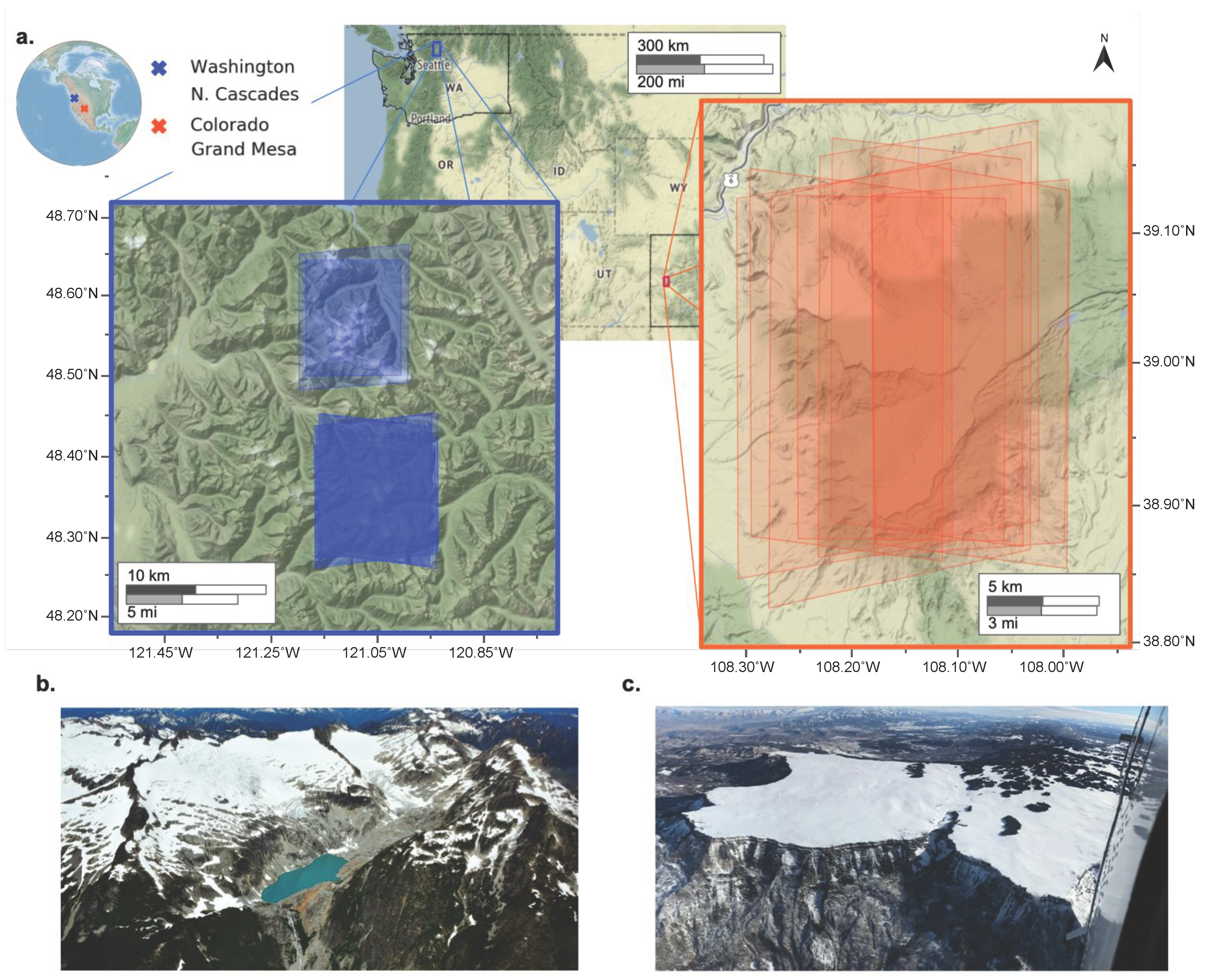
2.1. Study Sites

We selected two snow monitoring sites in the Western US: the Washington North Cascade Range and Grand Mesa in Colorado (Figure 1). These two sites have distinct climates, topography, and land cover that produce different snow conditions. The North Cascades site is more challenging for optical snow observation compared to the Grand Mesa site, with increased cloud cover, terrain shadowing, and the presence of glacial ice and firn.

The North Cascade Range of the Washington state (Figure 1) site spans an elevation range of 430–2703 m a.s.l. from the river valley bottom to the mountain peaks. The exposed areas in this region are primarily schist, orthogneiss, and plutonic rocks [49]. Western hemlock, red cedar, and Douglas fir are the predominant tree species at lower elevations (below 800 m) while silver fir is found between 600–1300 m [50]. At higher elevations, mountain hemlock is mixed with subalpine meadows between 1200–1600 m [50], with alpine lakes between 1270–1749 m a.s.l.

This site is geologically complex with perennial snowfields and dozens of active glaciers, including the USGS benchmark South Cascade Glacier [51]. Winters in the Washington North Cascades are generally mild, with moisture-laden air from the Pacific Ocean [52,53] helping to generate warm, dense maritime snow [54] and some of the deepest snowpack in the Western U.S., with mean annual snowfall exceeding 15 m in some locations [55].

Grand Mesa, located in western Colorado, is one of the largest high-elevation, flat-topped mountains in the world (Figure 1a,c). Chosen as the primary site for NASA’s SnowEx campaigns, the mesa spans an elevation range of 3000–3400 m a.s.l., with a relief of 1800 m above the surrounding valley floor [56]. The mesa is dotted with lakes and reservoirs as well as isolated stands of Engelmann spruce and subalpine fir [57], which increase in density and coverage from west to east. The snow water equivalent (SWE) and elevation also increase from west to east [56]. The geology of the mesa includes a cap of volcanic basalt, with exposures of the Green River shale and Wasatch sandstone formations [58,59] on the surrounding hillslopes. During the accumulation season, prevailing maritime air masses coming from the Pacific generate cold, continental snowpack [60], with a mean annual snowfall of ~5–6 m [58].

2.2. Data

We obtained archived “System-ready” Level-1B (L1B) Maxar WorldView-2 and WorldView-3 satellite images acquired over our study sites between 2015 and 2019 under the NGA NextView license (

Table 1. Metadata for WorldView-2 (WV-2) and WorldView-3 (WV-3) images analyzed in this study. Ground sample distance (GSD) is a measure of the ground-projected distance between the center of two adjacent pixels.

Location	Date	Sensor	Catalog ID	Mean Sun Elevation	Mean Sun Azimuth	Mean Satellite Elevation	Mean Satellite Azimuth	Mean Off-Nadir Viewing Angle	PAN GSD [m]	MS GSD [m]
WA N Cascades	20 May 2015	WV-3	104001000C1BB800	60.0°	157.2°	58.5°	196.4°	28.3°	0.39	1.55
			104001000CB3D400	60.0°	156.7°	82.7°	6.6°	6.9°	0.31	1.25
WA N Cascades: South Cascade Glacier	24 April 2018	WV-3	104001003B034600	53.8°	162.7°	63.5°	145.3°	23.8°	0.36	1.45
			104001003B7AC300	53.8°	162.3°	61.4°	54.2°	26.0°	0.37	1.50
	27 May 2018	WV-3	104001003D88B900	63.0°	171.7°	61.7°	318.2°	25.7°	0.37	1.49
			104001003DD34200	63.0°	172.2°	58.9°	246.9°	28.0°	0.39	1.54
	5 May 2019	WV-3	104001004C8CF300	56.6°	158.2°	58.1°	132.6°	28.7°	0.39	1.57
			104001004CBC0600	56.6°	157.8°	58.8°	72.2°	28.3°	0.39	1.55
CO: Grand Mesa	1 February 2017	WV-3	1040010026C28A00	31.9°	160.5°	62.3°	137.0°	24.9°	0.37	1.47
			10400100276B9500	31.9°	160.2°	57.1°	52.7°	29.9°	0.40	1.59
			1040010028192C00	32.0°	160.7°	56.9°	152.4°	29.6°	0.40	1.59
			10400100286A3900	31.9°	160.4°	63.3°	65.7°	24.2°	0.36	1.45
	3 April 2018	WV-2	103001007A0DBD00	53.7°	290.0°	78.9°	109.4°	10.0°	0.48	1.91
			103001007B395800	53.7°	210.2°	52.7°	28.1°	33.5°	0.65	2.59
	26 March 2019	WV-3	1040010048434C00	52.3°	163.4°	62.7°	315.7°	24.9°	0.37	1.47
			104001004918EB00	52.3°	163.8°	55.8°	236.1°	30.7°	0.41	1.62

). All the images were collected as in-track stereo pairs, with both panchromatic (PAN, 450–800 nm) and 8-band multispectral (MS, 397–1040 nm) images. The off-nadir viewing angles ranged between 6.9° and 33.5° (Table 1) with corresponding ground sample distance (GSD) values between 0.31–0.65 m for PAN and 1.25–2.59 m for MS images. Some of the images (e.g., 24 April 2018) of illuminated snow-covered surfaces suffered from limited detector saturation due to overexposure. Supplementary Table S1 includes additional information on commercial VHR sensors including the available products, spectral coverage, and GSD for data products.

The WorldView-2 and WorldView-3 instruments include time-delay integration (TDI) linescan sensors with arrays of adjacent CCD detectors providing images across the full ~13–17 km wide swath. Each detector requires relative geometric and radiometric calibration, including dark offset subtraction and relative gain modifications, to produce the self-consistent Level-1B products. More information can be found in the technical note for WorldView-2 and WorldView-3 [61].

We orthorectified the WorldView images using the ⅓-arcsecond (~10 m) seamless digital elevation model (DEM) from the USGS 3D Elevation Program (3DEP, formerly known as the National Elevation Dataset) [62]. The 3DEP DEM basemap is a mosaic of terrain models with varying sources (i.e., airborne lidar and digitized contour maps) and collection dates (USGS, 2017). The source of the DEM timestamp for the Grand Mesa site (CO_MesaCo-QL2_2015) was 2016 and between 1958 and 2017 for the North Cascades site. We adjusted the 3DEP DEM datums to the ellipsoid using the dem_geoid utility from the NASA Ames Stereo Pipeline (ASP) [63,64].

3. Materials and Methods

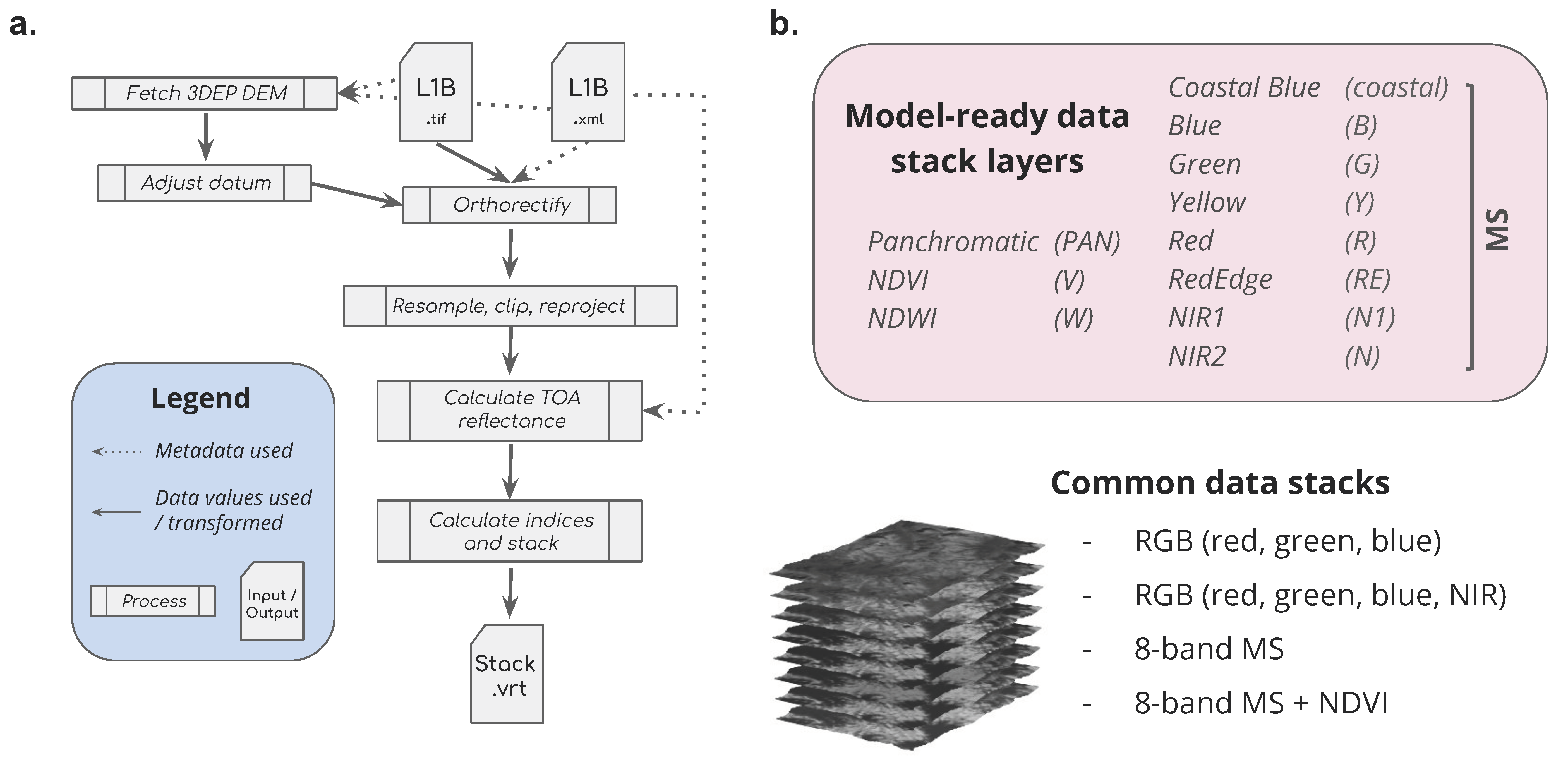
3.1. Pre-Processing

Figure 2a shows the general preprocessing workflow. We used the ASP mapproject utility with bilinear interpolation to orthorectify all PAN and MS L1B images to a common 1.2 m (for WorldView-3) or 2.0 m (for WorldView-2) grid using the rational polynomial coefficient (RPC) sensor models and the 3DEP DEM basemap with ellipsoid heights.

Additionally, we performed absolute radiometric corrections to convert the 11-bit L1B digital number (DN) values to top-of-atmosphere (TOA) radiance values for each band. We used the absolute calibration factors and effective bandwidths provided with the L1B metadata, along with the 2016v0.int version calibration adjustment factors (i.e., gain and offset) following the methodology outlined in Updike and Comp for WV-2 [65] and Kuester for WV-3 [61]. We then corrected for solar spectral irradiance to convert TOA radiance to TOA reflectance values. Any TOA reflectance values less than 0.0 or greater than 1.0 were clamped to 0.0 and 1.0, respectively. TOA values exceeding 1.0 amounted to less than 1.5% of any single image. As mentioned earlier, one of our primary objectives was to evaluate the performance of simple landcover-classification approaches for accurate snow-cover mapping using VHR stereo images. Thus, we did not attempt to convert the TOA reflectance products to higher-level surface reflectance products, which would require more complex models and corrections for atmospheric, topographic, and bidirectional reflectance distribution function effects. See Section 5.2 for further discussion of these issues.

We also calculated common spectral indices and included them in our data stacks (Figure 2) to mitigate the impacts of sensor calibration error and shading and atmospheric variability. We calculated normalized difference vegetation index (NDVI) values using the red (626–696 nm) and NIR 1 (765–899 nm) bands, and normalized difference water index (NDWI) [66] using the green (507–586 nm) and NIR 2 (857–1039 nm) bands.

3.2. Classification

3.2.1. Machine Learning Algorithm Selection and Model Implementation

After preliminary exploration and consideration of classification algorithms (e.g., support vector machines, Gaussian Processes, and artificial and convolutional neural networks), we chose the random forest algorithm [39] implemented in the scikit-learn Python package [67]. A random forest classifier leverages an ensemble of decision tree predictors to determine the class label for a given input. Preliminary testing ranged between 100 and 500 trees, but we observed little to no improvement in accuracy over the 100-tree configuration. As noted in the scikit-learn documentation, to control overfitting, the random forest implementation uses the highest average probability estimate from decision trees rather than majority voting to make class predictions. The final model parameters were 100 trees (n_estimators) with a square root maximum feature number (max_features) used for splitting and tree-building.

3.2.2. Model Input Configurations

We considered several variables when preparing the models: input data layer combination, time of year, and site/physiography of training images. All combinations of input data layers used to build the models are listed in

Table 2. Input data stack layer combinations for all models described.

Data Stack	Input Data Stack Layers
coastal_V	coastal, NDVI
coastal_VW	coastal, NDVI, NDWI
PAN_VW	panchromatic, NDVI, NDWI
RGB	red, green, blue
RGBN	red, green, blue, near infrared 2
RGBN_V	red, green, blue, near infrared 2, NDVI
MS	coastal, blue, green, yellow, red, red edge, near infrared 1, near infrared 2
MS_V	coastal, blue, green, yellow, red, red edge, near infrared 1, near infrared 2, NDVI
PAN_MS	panchromatic, coastal, blue, green, yellow, red, red edge, near infrared 1, near infrared 2
PAN_MS_V	panchromatic, coastal, blue, green, yellow, red, red edge, near infrared 1, near infrared 2, NDVI

.

Several different combinations of input data layers were created to emulate commonly available optical and near-infrared spectral combinations for earth-observing satellite sensors (e.g., RGB and RGBN, see Figure 2b). As these models used a subset of bands from the WV MS products, they are referred to as “limited band models.” These limited band models were included to assess the feasibility of using only a few spectral inputs to produce accurate land cover maps. Models trained using all eight MS bands (for both WV-2 and WV-3) as inputs are referred to as “8-band MS” models (e.g., MS, MS_V, PAN_MS, and PAN_MS_V). These models were constructed to leverage the full multispectral coverage available from Maxar VHR sensors.

For interpretation, models were also qualitatively subdivided into two categories based on the source of training data: single-scene or multiple-scene models. The single-scene models were trained on a data stack from a single date and location. These models were used to answer questions about models’ spatiotemporal transferability (i.e., generalization)—how the site and time of year impact trained model performance (Section 3.2.6). The multiple-scene model (M101) was trained on two input data stacks with different dates and locations (both North Cascades and Grand Mesa sites) with the full input of available spectral bands (i.e., PAN_MS_V) to assess training data expansion impacts on classification accuracy. Supplementary Table S2 provides details for the 155 model configurations we considered in this analysis, with their corresponding F-scores.

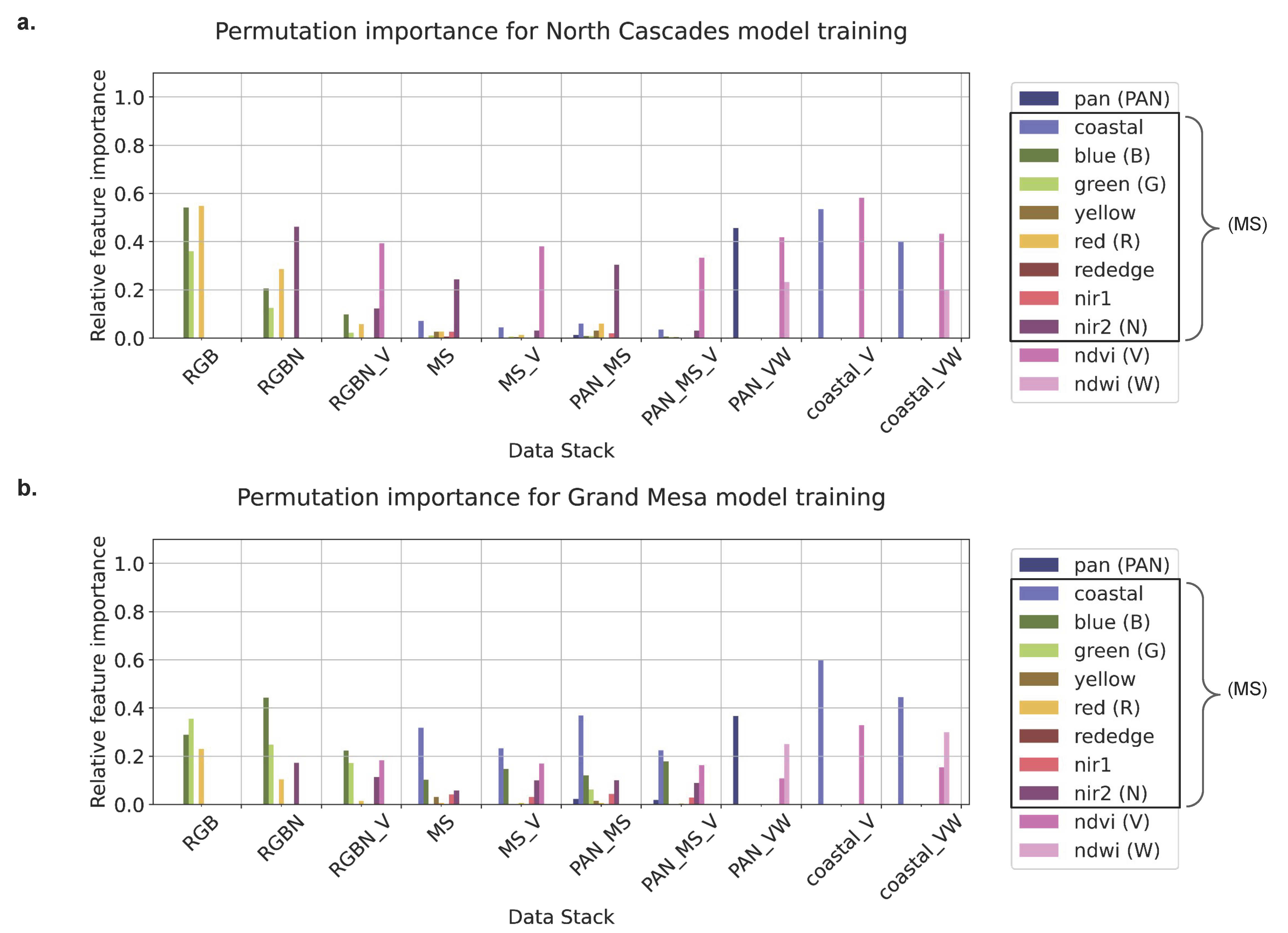
3.2.3. Feature Importance

Machine learning models with computable feature importance metrics, such as random forest, are useful for helping to identify the most important inputs, removing unimportant inputs, and reducing the feature space to balance computational efficiency with model performance. In this work, rather than reducing feature space, we primarily used feature importance to compare important inputs between different model configurations.

Both the Gini importance and permutation importance are implemented as feature importance metrics in scikit-learn. The Gini importance (mean decrease in impurity [MDI]) is a measure of how often a random pixel is incorrectly classified when given a random label according to the feature class label distribution. This makes the Gini importance strongly dependent on the class label distribution. Permutation importance (mean decrease in accuracy [MDA]) is the decrease in model score when a single feature class label is randomly shuffled and the linkage between data and label is deliberately broken. Through this shuffling, important features are identified as those that generate more error when intentionally mislabeled [68]. Despite the increased processing time required, we chose to analyze permutation importance (MDA) for its improved accuracy. Feature importance values were used to evaluate which inputs were consistently important for building models that could accurately classify land cover in the presence or absence of other input layers.

3.2.4. Training Data

Polygons outlining clusters of pixels for each feature class were manually delineated to use during model training for each unique image acquisition date (Table 1). We attempted to maintain uniform spatial distribution of polygons [69] (e.g., Supplementary Figure S1) and attempted to minimize classification bias by balancing feature classes [70] with ~65,000 pixels (~0.1 km² at 1.2 m GSD) per feature class. This was more challenging for snow-covered images with little exposed ground, surface water, and/or few clouds. Polygons were combined to create 3–6 different priority class labels: illuminated snow, shaded snow, vegetation, exposed ground, surface water, and cloud cover. In some cases, the number of feature classes varied with date; for example, the Grand Mesa model (26 March 2019; M17 in Supplementary Table S3) was trained with fewer feature classes than the North Cascades model (20 May 2015; M7 in Supplementary Table S3), as land and frozen water surfaces were heavily snow-covered. When exposed ground was visible at the Grand Mesa site, training polygons were focused on shale and sandstone units, as the basalt cap was covered with snow or vegetation.

3.2.5. Accuracy Assessment

Model development involved a train/val/test split of 70% training, 15% validation, and 15% testing [71] for each unique image acquisition date, implemented in scikit-learn. We used 10-fold cross-validation to assess overall model performance (i.e., accuracy) and stability via Precision, Recall, and F-scores (Equations (1)–(3)). Weighted macro F-scores were calculated to account for any training label imbalances by “weighting” label metrics based on the number of true instances (i.e., support). We did not use Cohen’s Kappa, a traditional accuracy metric reported for land cover classifications, as other studies have indicated that it unnecessarily accounts for correct predictions due to chance [72,73,74,75].

$$Precision=\frac{True Positives}{True Positives+False Positives}$$

(1)

$$Recall=\frac{True Positives}{True Positives+False Negatives}$$

(2)

$$F=2\cdot \frac{Precision \cdot Recall}{Precision+Recall}$$

(3)

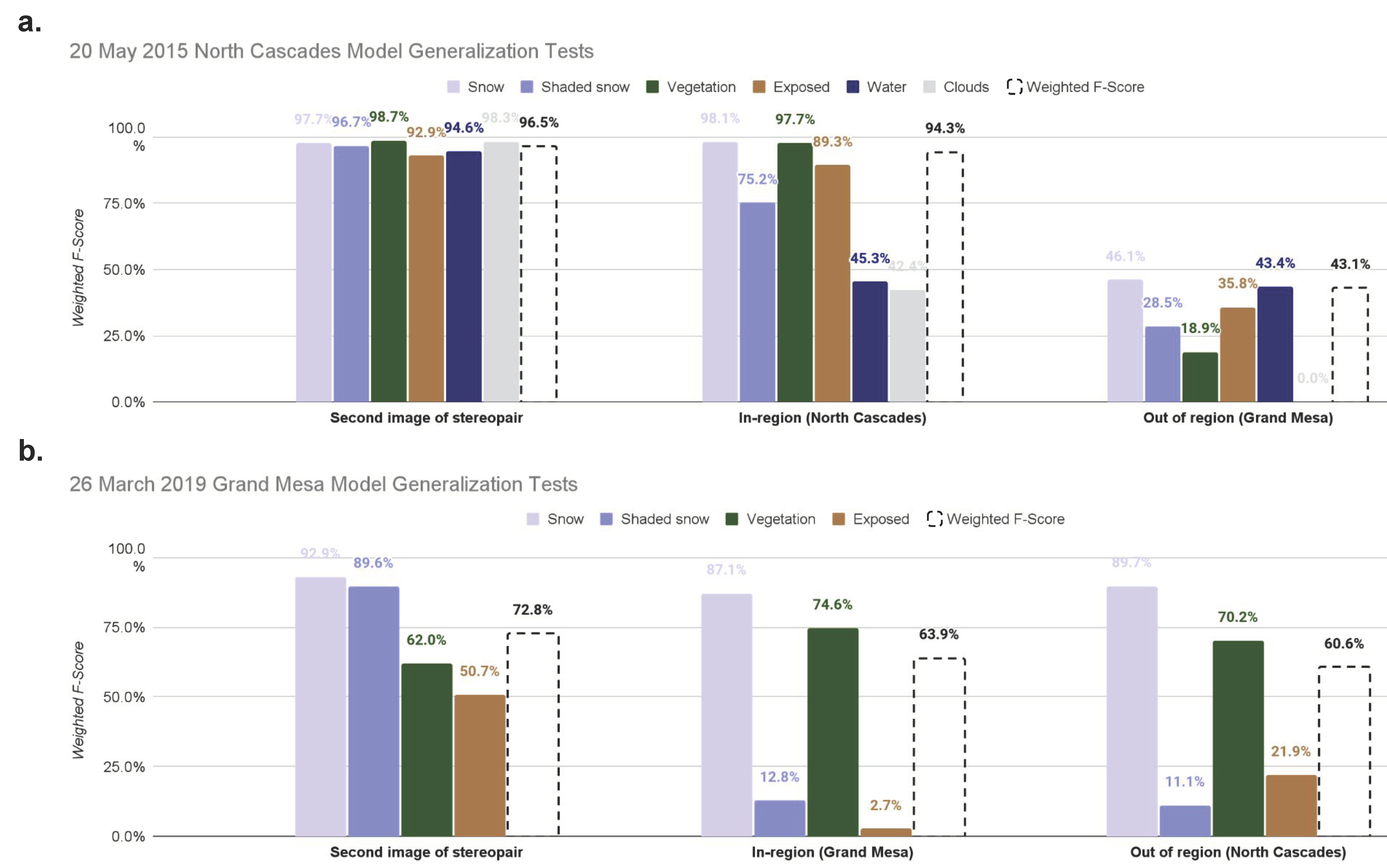
3.2.6. Model Transfer Tests and Generalization

We attempted to assess model generalization using our pre-trained models for new images, with the goal of reducing duplicate training effort. After training, testing, and validating models for a single image (i.e., single-scene models), we conducted model transfer tests using a “base model” with acquisition date that offered the best feature class distribution for each site. We used the M7 model (20 May 2015 image data stack) for the North Cascades site and the M17 model (26 March 2019 image data stack) for the Grand Mesa site base model. These tests were used to assess a single-scene model’s ability to generalize to images from the same physiographic region and images outside the physiographic region in which the model was trained. We also conducted similar model transfer tests using the multiple-scene model (M101) to assess generalization to new images, though all images were from the same physiographic region based on the inputs for the multiple-scene model.

We expected physiography to affect both initial snow grain conditions and subsequent redistribution, metamorphism, and snowmelt processes, all of which impact the reflectance of snow. Each image in Table 1 was assigned to either the North Cascades region or the Grand Mesa region. Acquisition dates were thus grouped together as follows: 24 April–27 May for the North Cascades site and 1 February–3 April for the Grand Mesa site. Images acquired as in-track stereopairs inherently shared the same day of year and physiography, near-identical solar illumination, but different viewing geometry than the M7 and M17 models. The M7 and M17 models were trained on stereo image data stacks for the smaller off-nadir view angle. We define the “first” stereo image in each stereopair as the image with the smaller off-nadir view angle and define the “second” as the image with the larger off-nadir view angle.

These qualitative categorizations were used to inform interpretation of overall model generalization performance. Supplementary Table S3 shows the full set of model transfer experiments and corresponding F-scores.

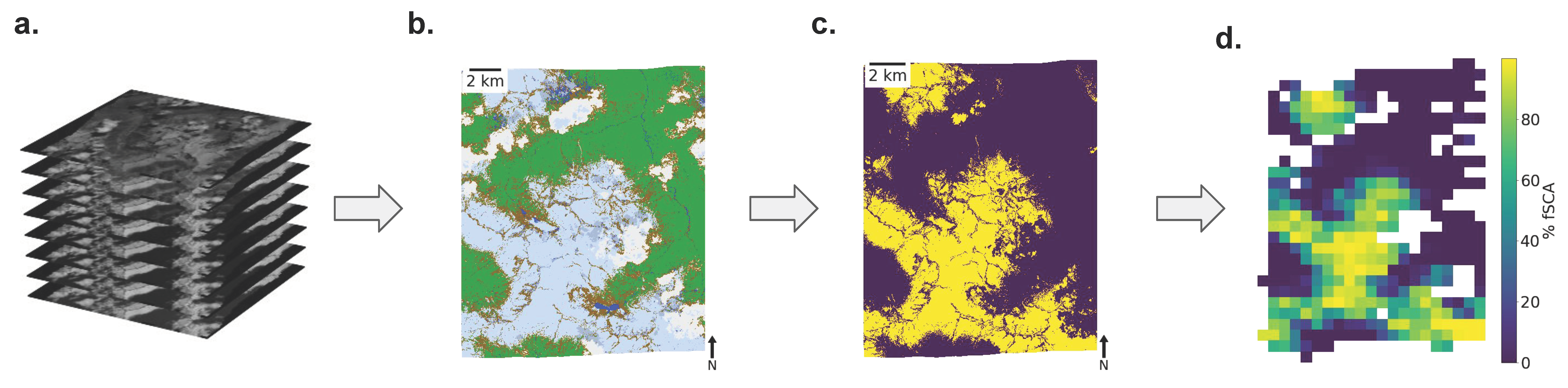
3.2.7. Snow Cover Products and Comparison with Other Snow Cover Datasets

To assess the quality of coarser-resolution fractional snow cover products, we downsampled our VHR land cover classifications to prepare fractional snow-covered area products (WV fSCA). First, we extracted binary snow cover from the random forest classification maps by assigning a value of 1 to pixels classified as snow or shaded snow and a value of 0 to all other non-snow classes (Figure 3a–c). We then reprojected and downsampled our VHR snow cover maps using an averaging algorithm to match the publicly accessible, “viewable” fractional snow-covered area products from MODIS (MODSCAG fSCA, ~500 m GSD) [28] and canopy-adjusted products from Landsat (Collection 1 fSCA, ~30 m) [76,77].

We created binary cloud masks using the VHR land cover classification and resampled these masks to produce WV cloud cover percentage products to match the coarser fSCA products. We excluded pixels with resampled cloud cover percentage values of 50% or higher. We also used the revised cloud mask products (REVCM) from Landsat and cloud flag values from MODSCAG and omitted these cloud-flagged pixels from analysis.

Finally, we subtracted the resampled, cloud-masked WV fSCA product from corresponding coarser resolution products to produce difference maps, and then calculated per-pixel statistics for each difference map and aggregated statistics for all difference maps at both sites (Supplementary Table S4). All products were reprojected to a local Universal Transverse Mercator (UTM) zone for visualization (Figure 3d).

We used the MODSCAG fSCA products from the same day as the corresponding WorldView image acquisition. The local time of observation for MODIS was ~10:30 AM +/− 5 min [78]. We used the viewable MODSCAG fSCA products for comparisons with our resampled WV fSCA products, as they identify snow cover that is unobstructed from the sensor’s view. The more recent “on-the-ground” STC-MODSCAG fSCA products [23] include additional corrections based on forest canopy to estimate occluded snow cover, but these products were not publicly available at the time of this analysis.

We used the Landsat Collection 1 fSCA products with the shortest possible temporal offset from the corresponding WorldView image acquisition (~2–5 days, Supplementary Table S4). The limited temporal offsets should not significantly impact our fSCA comparisons. There were no new precipitation events and no large wind events that could have resulted in substantial redistribution between Landsat and WorldView collections. The local time of observation for Landsat 7/8 was ~10:00 AM local +/− 15 min [79]. The Landsat Collection 1 fSCA products have all undergone canopy correction post-processing and are thus “on-the-ground” datasets. Viewable fSCA have since been made available for Collection 2, but these products were not released for our sites and acquisition dates at the time of this analysis.

We expected the canopy-corrected Landsat fSCA products to display greater differences over dense vegetation than the viewable MODSCAG fSCA or WV fSCA, although we recognized that the magnitude would vary based on the actual view angles for each of these sensors. To avoid potential issues related to view angle, we focused our comparisons on “open” areas, defined by a fractional vegetation cover product (WV fVeg) for subsequent aggregation. As with the WV fSCA products, we used a binary vegetation/non-vegetation classification approach followed by average downsampling to match coarser resolution fSCA product grids. Open areas were designated as pixels where WV fVeg < 25% and densely vegetated areas as pixels where WV fVeg ≥ 25%, broadly following the canopy-cover-density classes used by McGrath et al. [80].

We also compared per-pixel fSCA values for completely snow-free (0% fSCA) or completely snow-covered (100% fSCA) pixels to assess snow detection performance. This approach was adopted to minimize the impact of mixed pixels for fSCA comparison at the coarse sensor resolution, with the presence of only the snow endmember or complete absence of the snow endmember. Accurately detecting snow absence (i.e., completely snow-free pixels) is integral to calculating snow disappearance dates and constraining the surface albedo evolution for energy balance and hydrologic models [81]. Compared to intermediate fSCA (0% < x < 100% fSCA) values, we expected good agreement between the three fSCA products for completely snow-free and completely snow-covered pixels.

4. Results

4.1. Single-Scene Model Performance

The 10-fold cross-validated F-scores using the validation sets from the training data discussed in Section 3.2.4 show that the single-scene models generated accurate classifications with all model configurations, attaining F-scores of 84% or higher (Supplementary Table S2). The models trained with 8-band MS inputs (e.g., M7–M10 in Supplementary Table S2) displayed the highest accuracy (F-scores > 99%), with minimal class confusion and both precision and recall scores nearing 100%. Figure 4 shows the classification results for two of the base 8-band MS single-scene models (M7 and M17 in Supplementary Table S2) for each study site.

In general, the snow, shaded snow, and vegetation classes were correctly classified (e.g., Figure 4c). Exposed surfaces, cloud, and water classes were the most common feature classes for which the pixels were incorrectly classified (i.e., errors of commission). These misclassified pixels were located most often at the boundaries of feature classes (e.g., pixels between snow and exposed ground misclassified as cloud cover) and in dark, shaded areas with low reflectance values (which were misclassified as surface water).

The limited band models (e.g., M1–M6 in Supplementary Table S2) consistently produced lower classification accuracies than the models that included all eight MS bands (e.g., M7–M10 in Supplementary Table S2). The models trained with a single spectral band and normalized indices (i.e., PAN_VW, coastal_V, and coastal_VW, such as in M1–M3 in Supplementary Table S2) performed comparably with the models trained on data stacks without normalized indices (e.g., M4, M5 in Supplementary Table S2).

4.2. Single-Scene Feature Importance

Feature importance tests for the varying single-scene model data stack inputs indicated that the coastal blue and NDVI inputs were important for both study sites (Figure 5). When restricting the model training stacks to these two inputs, the classifications were less accurate than the 8-band MS models, but still performed quite well (F-scores: 97.7% vs. 99.8%). The models with five or fewer input layers relied more heavily on individual inputs than the models with more than five inputs.

We observed different feature importance proportions for the two sites. The RGB models for the North Cascades site showed that blue and red inputs were more important than the green input, while the RGB models for the Grand Mesa site showed the opposite. What is additionally noteworthy is the apparent importance of the coastal blue input in the Grand Mesa models for several different data layer configurations.

4.3. Model Transfer and Generalization

Single-scene models for the North Cascades and Grand Mesa sites (M7 and M17, respectively, Supplementary Table S2) were capable of limited generalization. The best model performance was observed when classifying a different image acquired for the same site during a similar time of year (i.e., the second image from an in-track stereopair for a model trained on the first image). As anticipated, the classification accuracy decreased when models were transferred and applied to images from different locations (Figure 6).

The models applied to the second image of an in-track stereopair (e.g., E1, E8, E15, and E22 in Supplementary Table S3) were the most accurate (F-scores: 96.5% in the North Cascades and 72.8% in Grand Mesa for M7 and M17 models, respectively) while the models applied to the in-region images (e.g., E2, E3 in Supplementary Table S3) had the second highest accuracy (F-scores: 94.3% in the North Cascades and 63.9% in Grand Mesa). Figure 6 shows the F-scores by feature class, ranging between 50.7–98.7% for the second image of an in-track stereopair, and much more widely (F-scores: 0–98.1%) for the other tests. The Grand Mesa model showed a good out-of-region performance for illuminated snow (average F-score: 89.7%), while the North Cascades model did not perform as well (average F-score: 46.1%).

The multiple-scene model (M101 in Supplementary Table S2), built from WV-3 images over both the North Cascades and Grand Mesa sites, performed better than any of the 8-band MS single-scene models for out-of-region transfer (Supplementary Figure S2, Supplementary Table S3). However, single-scene models produced more accurate classifications than multiple-scene models when employed in-region (Supplementary Figure S2), that is, for the second image of a stereopair or an image acquired on a different date for the same site. Based on the higher in-region transfer accuracy and single-scene stack accuracy presented in Section 4.1, we used the 8-band MS single-scene models (e.g., M7, M17, M27, M128, and M138 in Supplementary Table S2) for subsequent snow classification and fSCA comparisons.

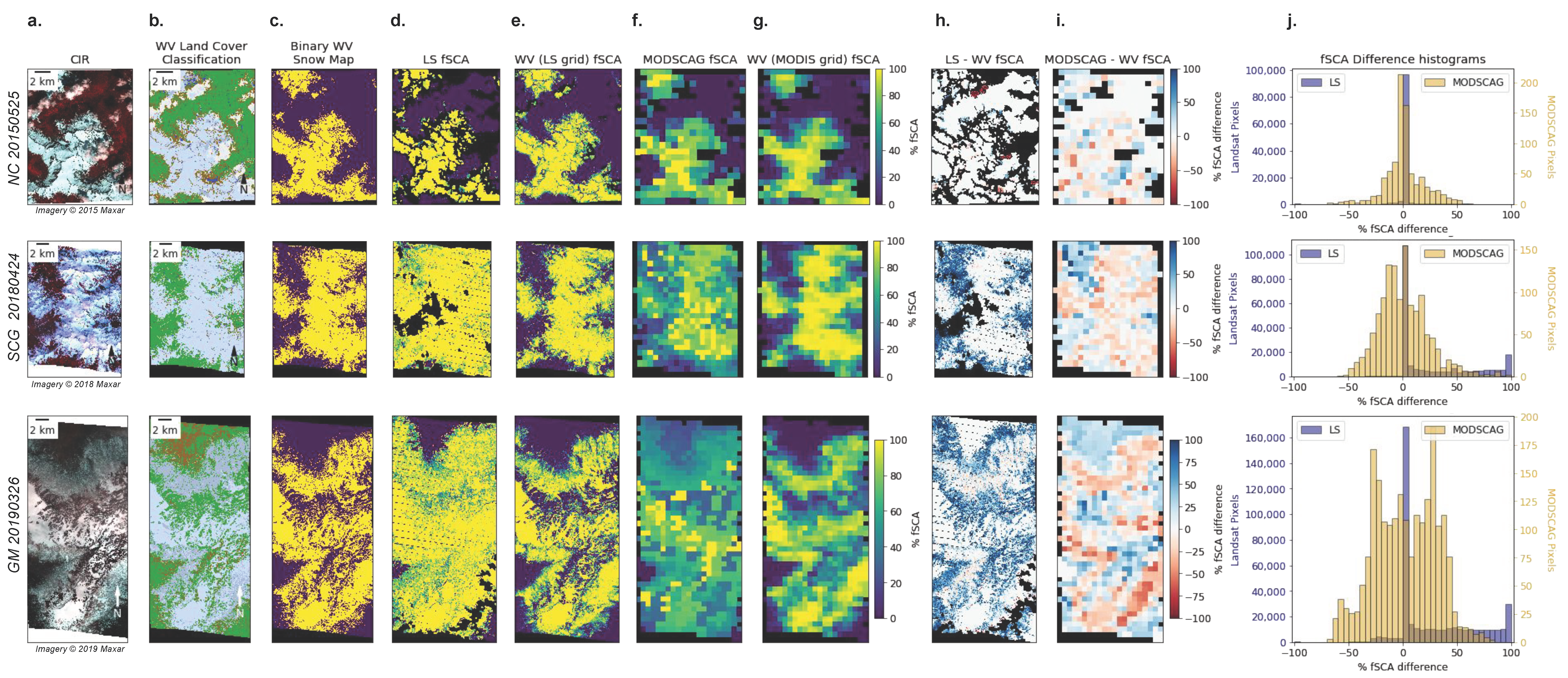
4.4. Snow Classification Comparisons

4.4.1. Qualitative Assessment of fSCA Difference

When compared to the downsampled WV fSCA products (Figure 7), both the Landsat and MODSCAG products showed higher fSCA values (e.g., Figure 7h,i, middle and bottom rows in blue) near areas classified as vegetation. The MODSCAG fSCA products showed differences in fSCA estimates over large areas classified as snow (Figure 7i). The largest fSCA differences were observed for the Grand Mesa site, where MODSCAG had higher fSCA values both on and off the mesa, and lower fSCA values on adjacent slopes.

Due to the nature of the available VHR in-track stereo collections, most of the images in this study had mean off-nadir viewing angles larger than 20° (Table 1), which can result in occlusions near trees and high-relief terrain. Comparisons of the per-pixel fSCA values with only the smallest mean off-nadir viewing angle image (CATID: 104001000CB3D400, off-nadir viewing angle: 6.9°) showed smaller fSCA differences (Supplementary Figure S3). Supplementary Figure S3 shows individual difference maps and histograms for all the comparisons in Supplementary Table S4.

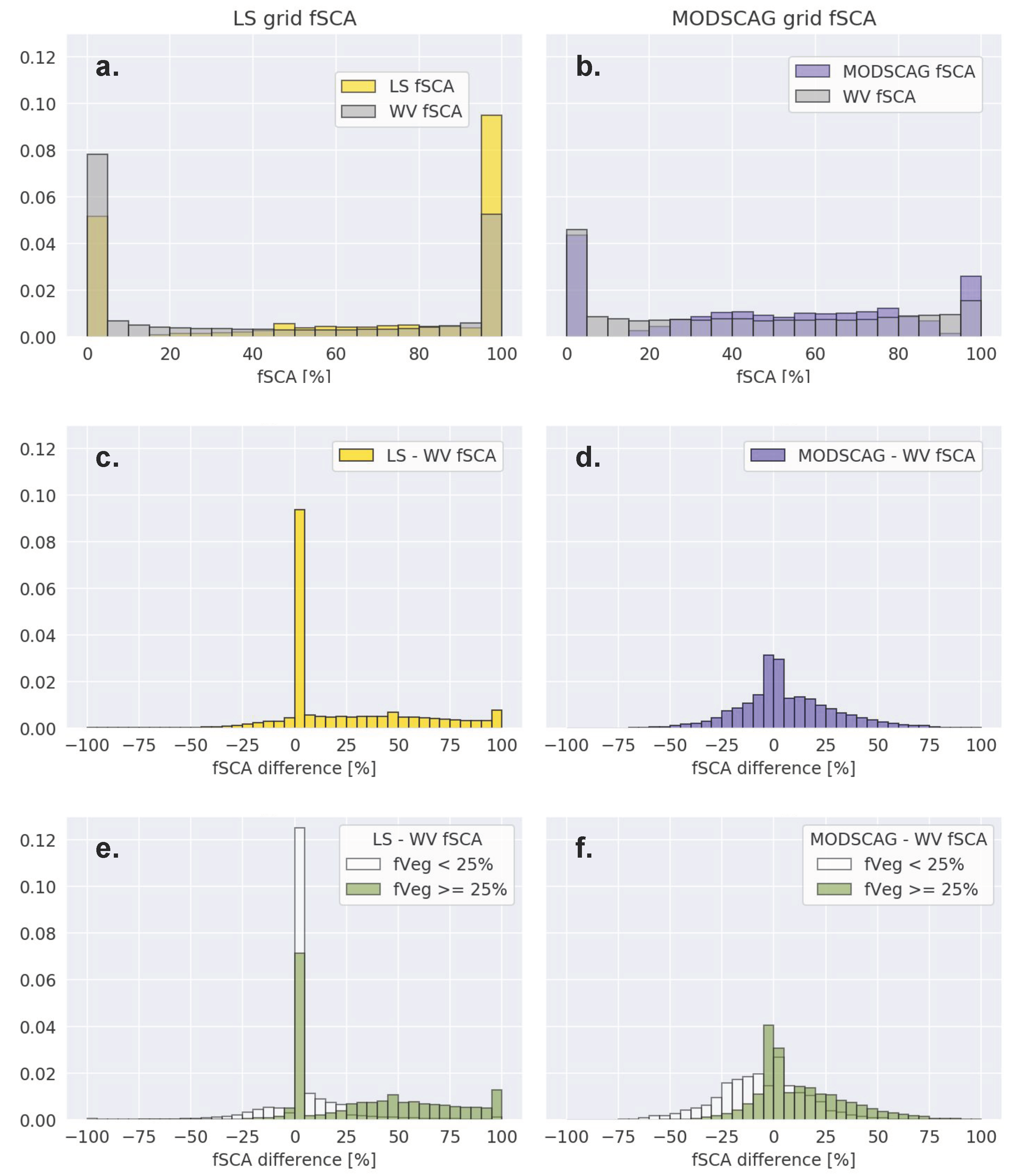
4.4.2. Quantitative Assessment of Aggregated fSCA Difference

The aggregation of all fSCA difference products for both sites and all time periods (Supplementary Figure S3) showed good agreement between the coarse resolution fSCA products and the downsampled WV fSCA products (Figure 8). In the aggregate, the median difference was 0% for both Landsat fSCA and MODSCAG fSCA, but both products had slightly positive mean fSCA differences (Landsat mean of 14% and MODSCAG mean of 7%; Supplementary Table S5, Figure 8c,d).

Further analysis over open the areas defined using the WV fractional vegetation cover (WV fVeg < 25%, see Section 3.2.7) showed no median difference (0%) between Landsat and WV fSCA and a small negative median difference (−2%) between MODSCAG and WV fSCA (Figure 8e,f, Supplementary Table S5). Over dense vegetation (WV fVeg ≥ 25%), both Landsat and MODSCAG fSCA (Figure 8e,f, Supplementary Table S5) showed higher median difference values (Landsat median of +25% and MODSCAG median of +5%). While the measures of spread were relatively stable for MODSCAG fSCA (~20–25%), the standard deviation and interquartile range (IQR) of the fSCA difference values was much lower for the Landsat fSCA estimates over open areas compared to densely vegetated areas (SD—19% vs. 35% and IQR—4% vs. 62%, respectively).

The analysis of the completely snow-covered pixels (100% fSCA) showed that both Landsat and MODSCAG fSCA products identified more snow-covered pixels than WV fSCA (Supplementary Table S6). Out of the 26,315 valid fSCA values for the common MODSCAG grid, MODSCAG identified 3418 pixels with 100% fSCA, while WV identified 257 pixels with 100% fSCA. In other words, MODSCAG overestimated the number of snow-covered pixels by a factor of 13.3. Out of the 4,515,817 valid fSCA values for the common Landsat grid, LS identified 2,090,153 pixels with 100% fSCA while WV identified 927,935 pixels—LS overestimated the number of completely snow-covered pixels by a factor of 2.3.

Analysis of the completely snow-free pixels (0% fSCA) showed that MODSCAG identified 2.7 times as many pixels as WV (MODSCAG—5717; WV—2139). Conversely, the Landsat fSCA products identified nearly the same number of pixels as WV (~0.8×; LS—1,165,256; WV—1,416,735), slightly underestimating the number of snow-free pixels.

5. Discussion

VHR land cover classification maps with short repeat time intervals can enable quantitative analyses of rapidly changing landscapes. These detailed maps can be used to delineate feature classes of interest (e.g., snow, vegetation, and exposed surfaces), track their evolution, and evaluate/improve the accuracy of coarser land cover and snow cover products. Beyond these tasks, accurate single-scene land cover classifications offer valuable, dense labels for training deep learning models [82].

5.1. Single-Scene Models

Our results show that the single-scene random forest model configurations produced accurate snow and land cover classification maps using WV images for both study sites. Despite the higher resolution and fewer mixed pixels compared to the coarser resolution products, the qualitative assessment of the WV classifications indicated that the misclassification of mixed pixels (e.g., pixels along two feature class boundaries) remains a challenge. The feature importance tests highlighted the importance of the NDVI input across the single-scene models trained at each of the sites. At both sites, the limited band models produced classifications with accuracies comparable to those produced by the 8-band models. This suggests that despite the limitations in multispectral coverage, sensors with high radiometric quality and fine spatial resolution may still produce broad land cover classifications at accuracies that compete with more extensive spectral coverage.

Despite attempts to define small, well-distributed training data polygons, the semivariogram tests for each feature class indicated that the reflectance values and single-scene accuracy assessments were affected by spatial autocorrelation in the training data. The common practice of using a random cross-validation approach for our single-scene accuracy assessments resulted in inflated accuracy scores of >99%, as has been documented elsewhere [83]. To gauge the impact of this spatial autocorrelation, we created a separate set of test polygons spaced several hundred to several thousand meters from the initial polygons. Using the original models to classify these test polygons (Supplementary Figure S4), new accuracy assessments indicated F-scores of ~94% for the North Cascades model (M7) and ~82% for the Grand Mesa model (M17), which are more representative of the models’ performance.

5.2. Model Transfer and Generalization

In the model transfer tests, single-scene models performed well on similar images (i.e., similar physiography and illumination conditions) but did not generalize well to out-of-region images. The differing performance between the models (Section 4.3) can be attributed to the differences in the acquisition dates, the number of feature classes, and terrain-induced spectral variability within the feature classes. The topography of Grand Mesa and its influence on snow distribution may have also contributed to the differences in spectral variability of the training data and resulting model transfer. The consistently strong performance of the Grand Mesa model for classifying illuminated snow (Figure 6, F-scores > 87%) could have resulted from capturing a wider range of spectral variability for the illuminated snow class over open, windblown surfaces on the mesa. Its consistently poor performance in classifying both in-region and out-of-region shaded snow (Figure 6; F-scores < 20%) could have arisen from a smaller range in spectral variability due to the relative scarcity of shaded snow in the Grand Mesa images.

Overall, the transfer tests using the multiple-scene model showed better performance across for both sites than the single-scene models transferred to out-of-region images (Supplementary Figure S2). However, the single-scene models still outperformed the multiple-scene models when deployed in the same physiographic region as the model training site (Supplementary Figure S2). Both single-scene models (M7 and M17) had strong in-region performance, outperforming the multiple-scene model (M101), and possessed differing feature importance metrics, suggesting that regionally specific models may be more attainable than a global model [84] when seeking strong generalization performance and accurate classification.

Our feature importance analysis (Section 3.2.3) also showed differences between sites, especially for the coastal blue band, the NIR2 band, and the NDVI inputs. The apparent importance of the coastal blue band across the model configurations could be partially related to the susceptibility of this shorter wavelength band (397–454 nm) to downwelling scattering and increased reflected path radiance, especially from neighboring snow pixels, which are not accounted for in the TOA reflectance values.

Although it should have minor impacts on the variation of reflectance within the feature classes, atmospheric corrections to obtain surface reflectance (rather than top-of-atmosphere reflectance) may help reduce some variability in the absolute feature class reflectance values between images. Additionally, corrections for the topographic, view, and illumination effects are important in areas of rugged terrain [85,86] and may help to reduce reflectance variability within feature classes for improved model generalization and land cover classification. Using a hierarchical series of binary classifiers [87] rather than a single classifier for multiple feature classes could also improve model generalization by simplifying the classification tasks.

5.3. Snow Classification Comparisons

The VHR snow cover (SCA and fSCA) observations currently offer the finest spatial resolution products available for our study sites and may serve to complement coarser fSCA products with a better temporal resolution, spatial coverage, and historical archives. Our aggregate analyses showed good agreement between both the Landsat and MODSCAG fSCAs when compared to the WV fSCA over open areas. The Landsat fSCA had a particularly small IQR while both coarser resolution products had near-zero median differences. Larger off-nadir view angles arising from the in-track stereo collection strategy impacted WV viewable snow cover near trees and in areas of high relief, just as with oblique perspectives near the edges of the MODIS swath and corners/edges of the Landsat images [23,88]. This means that despite good overall agreement in the viewable snow cover, both the MODSCAG fSCA and WV fSCA underestimated the true amount of snow cover in the areas of dense vegetation due to occlusions. These findings highlight the significance of sensor view angle impacts for forest-snow analysis [89] as well as the importance of adjusting for canopy cover [23] to accurately estimate snow cover using MODIS. Future efforts to minimize off-nadir acquisition geometry and implement canopy corrections for VHR images could improve overall snow-cover-mapping accuracy.

The assessment of completely snow-free (0%) and completely snow-covered (100%) fSCA values showed that both coarser resolution products overestimated the number of completely snow-covered pixels (LS: ~2×; MODSCAG: ~13×), suggesting that despite the near-zero median per-pixel differences, the coarser products evaluated here tended to overestimate the total fractional snow cover for the full scene. While the MODSCAG products also overestimated the completely snow-free pixels to a lesser extent (~2.7×), the Landsat fSCA products more accurately identified these pixels and only slightly underestimated the number of snow-free pixels (~0.8× as many pixels as WV fSCA). Our initial analysis suggests that the Landsat fSCA may better characterize both completely snow-covered pixels and completely snow-free pixels than the MODSCAG fSCA, though a more detailed consideration of viewable vs. canopy-corrected products for additional sites/times is warranted. Fusion products leveraging the spatial resolution of satellites such as Landsat and Sentinel and the temporal coverage of sensors such as MODIS and VIIRS [78,90,91] may offer further improvements. These approaches could reduce snow-cloud discrimination errors, provide finer resolution observations on shorter timescales, and generate a longer and denser time series for evaluation. While not evaluated here, the VIIRS binary snow cover products posted at 375 m [78] and the spectral unmixing fractional snow cover products posted at 1 km [91] may provide continuity for daily global snow observations as MODIS is decommissioned.

5.4. The Need for Fine-Scale Snow Cover

Fine-scale remote sensing observations are needed to accurately monitor changes in snow cover at critical locations and times. Along with the spatial boundaries of different land cover classes (e.g., near forest edges and within forest gaps), observing seasonal boundaries is also important. In late summer, sparse snow cover in the form of snow patches and drifts [33,92] support plant communities, maintain alpine meadows [93], and can be used as indicators of climate change [94]. In addition to shaping plant species diversity and distribution, snow patches can determine the timing and quantity of hydrologic and nutrient inputs [95,96,97].

These patches can have outsized impacts, but can be challenging to observe with spaceborne sensors, which can result in inaccurate hydrologic modeling outputs. Budd Creek, an ephemeral stream in California’s Sierra Nevada range, surrounded by granite peaks, exemplifies this issue (J. Lundquist, personal communication). Draining a northeastern cirque, late season streamflow in Budd Creek is sustained by snow-filled fissures and adjoining snow drifts. Small patches of snow are not easily detectable by 500 m MODSCAG fSCA products [30,91], as they likely occupy small percentages of any given pixel. Though The Landsat fSCA products offer an improvement by showing later snow disappearance dates, these products are also unable to detect snow later in the season as Budd Creek continues flowing.

The fine-scale snow mapping approaches presented in this work could provide the observations necessary for detecting these small, ecosystem-sustaining snow patches. As the climate continues to warm, these outliers of late snow disappearance may grow in ecohydrological importance, controlling biotic range shifts and buffering temperature fluctuations to become the climate refugia of the future [98,99,100].

5.5. Limitations and Considerations

One of the greatest strengths of WorldView-2 and WorldView-3 images—fine resolution—also presents one of the largest challenges for model transfer. The spatial variability of reflectance values for most surfaces is inherently linked to the spatial (and radiometric) resolution of the image. Though small pixels result in less spectral mixing from fewer feature classes in each pixel, there is also a wider range of reflectance values within each feature class. In other words, where unmixing methods are needed for other images, the WorldView-2 and WorldView-3 images can capture detailed surface properties—whether the snow is clean or dirty, whether the exposed surfaces are rock or soil, whether the trees are coniferous or deciduous, etc.

When aggregating these features with broad labels (i.e., snow, vegetation, and exposed), each feature class then contains more diverse values than what is observed and observable with coarse-resolution sensors. This makes a wide-ranging coverage of feature class representation an important consideration when generating training data for machine learning models. A two-stage approach would likely improve model transfer, employing an initial evaluation stage to focus classification efforts in generating large datasets that more adequately represent intra-class heterogeneity. Generating synthetic datasets based on these datasets by systematically perturbing values for each band (i.e., data augmentation) may also improve generalization.

While the relatively high accuracy of these simple random forest model configurations for a handful of land cover classes is encouraging, validation sets need to be made more rigorous for the widely varying reflectance within feature classes. One approach is to assign labels pixel by pixel rather than by polygons. While more efficient, polygon-based delineation potentially captures more uniform spectral reflectance within a polygon than a comparable number of randomly selected, individually labeled pixels. A preferable compromise may be to use a patch of pixels with a standard size to randomly select batches of single feature classes to label. Furthermore, stratifying the training and test sets via block cross-validation is recommended to eschew biased non-spatial cross-validation in the accuracy assessments [101].

The wide range and variability of observable reflectance values in our VHR images suggests that feature class expansion (more and narrower classes) could improve model accuracy, though potentially at the expense of model generalization. In other words, the number of feature classes needs to increase to manage larger ranges in the individual pixel reflectance values arising from a finer pixel resolution. In the case of accurately mapping small snow patches and snow boundaries, enumerating more targeted feature classes is preferable as there will be a larger proportion of boundary pixels with more distinct spectral signatures than those found in spatially contiguous areas of open snow. Extra care and attention in the training data curation is needed for areas with a rapidly changing snow presence (e.g., wind-scoured landscapes, ablation near the snowline during spring, etc.).

Traditional approaches rely on expert knowledge or unsupervised methods, which present challenges to including more training data. While the size of each VHR image (10⁸–10⁹ pixels per band for 1.2 m WorldView-3 MS products) precludes manually labeling each pixel, unsupervised methods such as spectral clustering can result in dozens of clusters within a single feature class that still require manual aggregation and labeling [48]. Though there are existing datasets that could be used to derive land cover feature class labels, such as the 30 m National Land Cover Database [102], these products are too coarse, outdated, or insufficiently labeled (i.e., they do not capture or represent seasonal snow or clouds as thematic classes) for our purposes. Potential solutions to the “training data bottleneck” include crowd-sourcing methods [103], attempts to adapt pre-existing labeled datasets [104], and weak labeling approaches [105]. The deep learning approaches developed by Cannistra et al. [106] and John et al. [107] produce binary snow cover maps from 3 m PlanetScope imagery using convolutional neural networks trained on thresholded aerial lidar snow-depth products. As mentioned earlier, the training requirements for neural networks greatly exceed those for random forest models—Cannistra et al. [106] trained their models on 370 million pixels compared to our ~65,000 samples per land cover class (~400,000 training pixels per model). Regardless of the machine learning approach applied, sufficiently representative and accurate training data labels for land cover beyond the built environment remains the primary challenge for accurate VHR optical land cover classifications.

A lesser confounder for model classification and transfer has been the magnitude and distribution of saturated pixels in the input data stack layers. In every combination of input layers, saturated regions in some bands have resulted in misclassification of the regions with extremely bright snow as clouds and vice versa. Dai and Howat [108] documented these saturation “striping” issues in the Level-1B WorldView images that can propagate to land-cover classification outputs. Though a few of our images were affected by these issues (Supplementary Figure S5), we observed limited impacts, such as classifying areas of relatively uniform snow features in one strip as ‘shaded snow’ and in another strip as ‘illuminated snow’.

To develop robust pixel-based models capable of accurately classifying multiple land-cover classes in VHR images from different seasons, locations, and illumination conditions, we recommend exploring:

• Improved preprocessing routines to obtain reliable absolute-surface-reflectance values for inter-image comparison;
• A larger library of training data (i.e., more labeled images to cover the range of reflectance values within each class);
• Simplified classification via hierarchical binary models;
• Regionally specific models over global models.

These improved models can then be deployed for operational seasonal-snow monitoring, which in turn will offer a growing library of training data from which to adaptively improve the models. Adopting approaches from the field of computer vision for remote-sensing science transcend employing the latest machine learning techniques and algorithms. As we strive to imbue domain relevance and physical meaning into model assessment metrics, we must also generate benchmark datasets, training sets, and create baseline models upon which we can iterate and improve as a community.

5.6. Operational Potential of WorldView-2 and WorldView-3 Snow Cover Products

Operational snow cover products need to be timely, accurate, reliable, and accessible [17,109]. We demonstrated that the accurate pixel-based classification of snow in WorldView-2 and WorldView-3 images is possible without SWIR bands, but our current models are limited in their generalizability. Figure 9 shows the cloud-free archive of WV-2 and WV-3 images collected between 2009 and 2020 for the Western U.S., which can potentially provide such a sample of seasonal snow cover across the region.

It is important to remember that most VHR satellites are tasked—collecting images for predetermined points and areas—and do not constantly acquire regular images over systematic paths and rows such as Landsat or Sentinel-2. With strategic tasking for areas of interest at critical times of year, VHR images have the potential to provide fine measures of snow cover. Furthermore, the in-track stereo collections analyzed here offer two viewing perspectives to observe clouds and other feature classes, which can be combined to provide a measure of uncertainty characterization for the resulting classification products. Finally, beyond snow cover, the in-track stereo collections can also offer precise snow depth measurements [47,80], enabling many additional applications.

6. Conclusions

Very-high-resolution images from WorldView-2 and WorldView-3 provide new opportunities and approaches for the detailed satellite mapping of seasonal snow cover in mountainous terrain, with many spectral bands and native image GSDs of 0.31, 1.2 m, and 3.7 m for PAN, MS, and SWIR bands, respectively. However, these detailed images involve large data volumes that prohibit manual analysis and flexible machine-learning approaches are required for large VHR satellite image archives.

We developed a suite of pixel-based classification models to better understand the potential for deriving land cover maps and snow cover products from WV images. We show that there is considerable potential for using random forest models to create classification maps (for a subset of priority land cover classes) that can accurately map snow cover to complement and evaluate coarser resolution products. Even when limited to a few spectral band inputs, these RF models offer a high accuracy for snow, suggesting that images collected at fine spatial and radiometric resolutions could overcome limited spectral coverage, provided that the spectral bands are strategically located.

We observed the best model generalization performance for images from the same site and a similar time of year, with the highest accuracy in the illuminated snow class and the vegetation class for all the transfer tests, especially at the Grand Mesa site. Variability in feature class reflectance likely contributed to the poor performance with the attempted out-of-region model transfer, and this intra-class variability remains a challenge to developing a single, highly accurate, and robust multi-class land cover classification model for VHR images. Such a model will likely require larger libraries of training data, simplified feature classes, and potentially regional and seasonal specificity.

Comparisons of the completely snow-free and completely snow-covered WV fSCA pixels showed that both the Landsat and MODSCAG fSCA products identified many more completely snow-covered pixels when compared to the downsampled WV fSCA products (2× and 13×) but that the Landsat fSCA products more closely estimated the number of completely snow-free pixels than MODSCAG fSCA (~0.8× vs. 2.7×). Aggregate comparisons of all WV fractional snow cover products with coarser resolution fSCA products showed good agreement over open areas. The differences in the fSCA over dense vegetation between the three products can be partially attributed to differences in the viewing geometry and canopy correction approaches. Future snow cover analyses using VHR images should prioritize smaller off-nadir view angles and canopy correction to minimize such issues. Regardless, the growing archives of VHR satellite images offer potential for global seasonal snow observation, measurement, and monitoring efforts as both standalone products and when combined with complementary coarser resolution observations.

References

1. Bales, R.C.; Molotch, N.P.; Painter, T.H.; Dettinger, M.D.; Rice, R.; Dozier, J. Mountain Hydrology of the Western United States. Water Resour. Res. 2006, 42. [Google Scholar] [CrossRef]
2. Viviroli, D.; Dürr, H.H.; Messerli, B.; Meybeck, M.; Weingartner, R. Mountains of the World, Water Towers for Humanity: Typology, Mapping, and Global Significance. Water Resour. Res. 2007, 43. [Google Scholar] [CrossRef]
3. Jones, H.G. The Ecology of Snow-Covered Systems: A Brief Overview of Nutrient Cycling and Life in the Cold. Hydrol. Process. 1999, 13, 2135–2147. [Google Scholar] [CrossRef]
4. Steltzer, H.; Landry, C.; Painter, T.H.; Anderson, J.; Ayres, E. Biological Consequences of Earlier Snowmelt from Desert Dust Deposition in Alpine Landscapes. Proc. Natl. Acad. Sci. USA 2009, 106, 11629–11634. [Google Scholar] [CrossRef]
5. Walker, D.A.; Halfpenny, J.C.; Walker, M.D.; Wessman, C.A. Long-Term Studies of Snow-Vegetation Interactions: A Hierarchic Geographic Information System Helps Examine Links between Species Distributions and Regional Patterns of Greenness. BioScience 1993, 43, 287–301. [Google Scholar] [CrossRef]
6. Winkler, D.E.; Butz, R.J.; Germino, M.J.; Reinhardt, K.; Kueppers, L.M. Snowmelt Timing Regulates Community Composition, Phenology, and Physiological Performance of Alpine Plants. Front. Plant Sci. 2018, 9, 114. [Google Scholar] [CrossRef]
7. Mankin, J.S.; Viviroli, D.; Singh, D.; Hoekstra, A.Y.; Diffenbaugh, N.S. The Potential for Snow to Supply Human Water Demand in the Present and Future. Environ. Res. Lett. 2015, 10, 114016. [Google Scholar] [CrossRef]
8. Elder, K.; Dozier, J.; Michaelsen, J. Snow Accumulation and Distribution in an Alpine Watershed. Water Resour. Res. 1991, 27, 1541–1552. [Google Scholar] [CrossRef]
9. Winstral, A.; Elder, K.; Davis, R.E. Spatial Snow Modeling of Wind-Redistributed Snow Using Terrain-Based Parameters. J. Hydrometeorol. 2002, 3, 524–538. [Google Scholar] [CrossRef]
10. Molotch, N.P.; Bales, R.C. Scaling Snow Observations from the Point to the Grid Element: Implications for Observation Network Design. Water Resour. Res. 2005, 41. [Google Scholar] [CrossRef] [Green Version]
11. Broxton, P.D.; Harpold, A.A.; Biederman, J.A.; Troch, P.A.; Molotch, N.P.; Brooks, P.D. Quantifying the Effects of Vegetation Structure on Snow Accumulation and Ablation in Mixed-Conifer Forests. Ecohydrology 2015, 8, 1073–1094. [Google Scholar] [CrossRef]
12. Mazzotti, G.; Essery, R.; Moeser, C.D.; Jonas, T. Resolving Small-Scale Forest Snow Patterns Using an Energy Balance Snow Model with a One-Layer Canopy. Water Resour. Res. 2020, 56, e2019WR026129. [Google Scholar] [CrossRef]
13. Berman, E.E.; Coops, N.C.; Kearney, S.P.; Stenhouse, G.B. Grizzly Bear Response to Fine Spatial and Temporal Scale Spring Snow Cover in Western Alberta. PLoS ONE 2019, 14, e0215243. [Google Scholar] [CrossRef] [PubMed]
14. Cosgrove, C.L.; Wells, J.; Nolin, A.W.; Putera, J.; Prugh, L.R. Seasonal Influence of Snow Conditions on Dall’s Sheep Productivity in Wrangell-St Elias National Park and Preserve. PLoS ONE 2021, 16, e0244787. [Google Scholar] [CrossRef] [PubMed]
15. Essery, R.; Pomeroy, J. Implications of Spatial Distributions of Snow Mass and Melt Rate for Snow-Cover Depletion: Theoretical Considerations. Ann. Glaciol. 2004, 38, 261–265. [Google Scholar] [CrossRef]
16. Thibault, I.; Ouellet, J.-P. Hunting Behaviour of Eastern Coyotes in Relation to Vegetation Cover, Snow Conditions, and Hare Distribution. Écoscience 2005, 12, 466–475. [Google Scholar] [CrossRef]
17. Hall, D.K.; Riggs, G.A.; Salomonson, V.V.; DiGirolamo, N.E.; Bayr, K.J. MODIS Snow-Cover Products. Remote Sens. Environ. 2002, 83, 181–194. [Google Scholar] [CrossRef]
18. Nolin, A.W. Recent Advances in Remote Sensing of Seasonal Snow. J. Glaciol. 2010, 56, 1141–1150. [Google Scholar] [CrossRef]
19. Giles, P. Remote Sensing and Cast Shadows in Mountainous Terrain. Photogramm. Eng. Remote Sens. 2001, 67, 833–839. [Google Scholar]
20. Dozier, J.; Painter, T.H. Multispectral and Hyperspectral Remote Sensing of Alpine Snow Properties. Annu. Rev. Earth Planet. Sci. 2004, 32, 465–494. [Google Scholar] [CrossRef]
21. Vikhamar, D.; Solberg, R. Subpixel Mapping of Snow Cover in Forests by Optical Remote Sensing. Remote Sens. Environ. 2003, 84, 69–82. [Google Scholar] [CrossRef]
22. Hall, D.K.; Riggs, G.A.; Salomonson, V.V. Development of Methods for Mapping Global Snow Cover Using Moderate Resolution Imaging Spectroradiometer Data. Remote Sens. Environ. 1995, 54, 127–140. [Google Scholar] [CrossRef]
23. Rittger, K.; Raleigh, M.S.; Dozier, J.; Hill, A.F.; Lutz, J.A.; Painter, T.H. Canopy Adjustment and Improved Cloud Detection for Remotely Sensed Snow Cover Mapping. Water Resour. Res. 2020, 56, e2019WR024914. [Google Scholar] [CrossRef]
24. Valovcin, F.R. Snow/Cloud Discrimination; Air Force Geophysics Laboratory: Hanscom Afs, MA, USA, 1976. [Google Scholar]
25. Hall, D.K.; Riggs, G.A. Accuracy Assessment of the MODIS Snow Products. Hydrol. Process. 2007, 21, 1534–1547. [Google Scholar] [CrossRef]
26. Selkowitz, D.J.; Forster, R.R.; Caldwell, M.K. Prevalence of Pure Versus Mixed Snow Cover Pixels across Spatial Resolutions in Alpine Environments. Remote Sens. 2014, 6, 12478–12508. [Google Scholar] [CrossRef]
27. Painter, T.H.; Dozier, J.; Roberts, D.A.; Davis, R.E.; Green, R.O. Retrieval of Subpixel Snow-Covered Area and Grain Size from Imaging Spectrometer Data. Remote Sens. Environ. 2003, 85, 64–77. [Google Scholar] [CrossRef]
28. Painter, T.H.; Rittger, K.; McKenzie, C.; Slaughter, P.; Davis, R.E.; Dozier, J. Retrieval of Subpixel Snow Covered Area, Grain Size, and Albedo from MODIS. Remote Sens. Environ. 2009, 113, 868–879. [Google Scholar] [CrossRef]
29. Rosenthal, W.; Dozier, J. Automated Mapping of Montane Snow Cover at Subpixel Resolution from the Landsat Thematic Mapper. Water Resour. Res. 1996, 32, 115–130. [Google Scholar] [CrossRef]
30. Hao, S.; Jiang, L.; Shi, J.; Wang, G.; Liu, X. Assessment of MODIS-Based Fractional Snow Cover Products over the Tibetan Plateau. IEEE J. Sel. Top. Appl. Earth Obs. Remote Sens. 2019, 12, 533–548. [Google Scholar] [CrossRef]
31. Cristea, N.C.; Breckheimer, I.; Raleigh, M.S.; HilleRisLambers, J.; Lundquist, J.D. An Evaluation of Terrain-Based Downscaling of Fractional Snow Covered Area Data Sets Based on LiDAR-Derived Snow Data and Orthoimagery. Water Resour. Res. 2017, 53, 6802–6820. [Google Scholar] [CrossRef]
32. Walters, R.D.; Watson, K.A.; Marshall, H.-P.; McNamara, J.P.; Flores, A.N. A Physiographic Approach to Downscaling Fractional Snow Cover Data in Mountainous Regions. Remote Sens. Environ. 2014, 152, 413–425. [Google Scholar] [CrossRef]
33. Parr, C.; Sturm, M.; Larsen, C. Snowdrift Landscape Patterns: An Arctic Investigation. Water Resour. Res. 2020, 56, e2020WR027823. [Google Scholar] [CrossRef]
34. Lundquist, J.D.; Lott, F. Using Inexpensive Temperature Sensors to Monitor the Duration and Heterogeneity of Snow-Covered Areas. Water Resour. Res. 2008, 44. [Google Scholar] [CrossRef]
35. Mott, R.; Schlögl, S.; Dirks, L.; Lehning, M. Impact of Extreme Land Surface Heterogeneity on Micrometeorology over Spring Snow Cover. J. Hydrometeorol. 2017, 18, 2705–2722. [Google Scholar] [CrossRef]
36. Thorn, C.E.; Hall, K. Nivation and Cryoplanation: The Case for Scrutiny and Integration. Prog. Phys. Geogr. Earth Environ. 2002, 26, 533–550. [Google Scholar] [CrossRef]
37. Currier, W.R.; Sun, N.; Wigmosta, M.; Cristea, N.; Lundquist, J.D. The Impact of Forest-Controlled Snow Variability on Late-Season Streamflow Varies by Climatic Region and Forest Structure. Hydrol. Process. 2022, 36, e14614. [Google Scholar] [CrossRef]
38. Marston, C.G.; Aplin, P.; Wilkinson, D.M.; Field, R.; O’Regan, H.J. Scrubbing Up: Multi-Scale Investigation of Woody Encroachment in a Southern African Savannah. Remote Sens. 2017, 9, 419. [Google Scholar] [CrossRef]
39. Breiman, L. Random Forests. Mach. Learn. 2001, 45, 5–32. [Google Scholar] [CrossRef]
40. Liu, C.; Huang, X.; Li, X.; Liang, T. MODIS Fractional Snow Cover Mapping Using Machine Learning Technology in a Mountainous Area. Remote Sens. 2020, 12, 962. [Google Scholar] [CrossRef]
41. Maxwell, A.E.; Warner, T.A.; Fang, F. Implementation of Machine-Learning Classification in Remote Sensing: An Applied Review. Int. J. Remote Sens. 2018, 39, 2784–2817. [Google Scholar] [CrossRef]
42. Jin, S.; Su, Y.; Gao, S.; Hu, T.; Liu, J.; Guo, Q. The Transferability of Random Forest in Canopy Height Estimation from Multi-Source Remote Sensing Data. Remote Sens. 2018, 10, 1183. [Google Scholar] [CrossRef] [Green Version]
43. Revuelto, J.; Billecocq, P.; Tuzet, F.; Cluzet, B.; Lamare, M.; Larue, F.; Dumont, M. Random Forests as a Tool to Understand the Snow Depth Distribution and Its Evolution in Mountain Areas. Hydrol. Process. 2020, 34, 5384–5401. [Google Scholar] [CrossRef]
44. Tsai, Y.-L.S.; Dietz, A.; Oppelt, N.; Kuenzer, C. Wet and Dry Snow Detection Using Sentinel-1 SAR Data for Mountainous Areas with a Machine Learning Technique. Remote Sens. 2019, 11, 895. [Google Scholar] [CrossRef]
45. Wu, W.; Li, M.-F.; Xu, X.; Tang, X.-P.; Yang, C.; Liu, H.-B. The Transferability of Random Forest and Support Vector Machine for Estimating Daily Global Solar Radiation Using Sunshine Duration over Different Climate Zones. Theor. Appl. Climatol. 2021, 146, 45–55. [Google Scholar] [CrossRef]
46. Marti, R.; Gascoin, S.; Berthier, E.; de Pinel, M.; Houet, T.; Laffly, D. Mapping Snow Depth in Open Alpine Terrain from Stereo Satellite Imagery. Cryosphere 2016, 10, 1361–1380. [Google Scholar] [CrossRef]
47. Deschamps-Berger, C.; Gascoin, S.; Berthier, E.; Deems, J.; Gutmann, E.; Dehecq, A.; Shean, D.; Dumont, M. Snow Depth Mapping from Stereo Satellite Imagery in Mountainous Terrain: Evaluation Using Airborne Laser-Scanning Data. Cryosphere 2020, 14, 2925–2940. [Google Scholar] [CrossRef]
48. Bair, E.H.; Stillinger, T.; Dozier, J. Snow Property Inversion from Remote Sensing (SPIReS): A Generalized Multispectral Unmixing Approach with Examples from MODIS and Landsat 8 OLI. IEEE Trans. Geosci. Remote Sens. 2020, 59, 7270–7284. [Google Scholar] [CrossRef]
49. Haugerud, R.A.; Tabor, R.W. Geologic Map of the North Cascade Range, Washington; Scientific Investigations Map 2940, 2 Sheets, Scale 1:200,000; 2 Pamphlets, 29 p. and 23 p.; U.S. Geological Survey: Tsukuba, Japan, 2009.
50. Kruckeberg, A.R. The Natural History of Puget Sound Country; University of Washington Press: Seattle, WA, USA, 1991; ISBN 978-0-295-97019-6. [Google Scholar]
51. O’Neel, S.; McNeil, C.; Sass, L.C.; Florentine, C.; Baker, E.H.; Peitzsch, E.; McGrath, D.; Fountain, A.G.; Fagre, D. Reanalysis of the US Geological Survey Benchmark Glaciers: Long-Term Insight into Climate Forcing of Glacier Mass Balance. J. Glaciol. 2019, 65, 850–866. [Google Scholar] [CrossRef]
52. Rasmussen, L.A.; Tangborn, W.V. Hydrology of the North Cascades Region, Washington: 1. Runoff, Precipitation, and Storage Characteristics. Water Resour. Res. 1976, 12, 187–202. [Google Scholar] [CrossRef]
53. Bach, A. Snowshed Contributions to the Nooksack River Watershed, North Cascades Range, Washington. Geogr. Rev. 2002, 92, 192–212. [Google Scholar] [CrossRef]
54. Trujillo, E.; Molotch, N.P. Snowpack Regimes of the Western United States. Water Resour. Res. 2014, 50, 5611–5623. [Google Scholar] [CrossRef]
55. Leffler, R.J.; Horvitz, A.; Downs, R.; Changery, M.; Redmond, K.T.; Taylor, G. Evaluation of a National Seasonal Snowfall Record at the Mount Baker, Washington, Ski Area; National Weather Digest: Norman, OK, USA, 2001; pp. 15–20. [Google Scholar]
56. Kim, E.; Gatebe, C.; Hall, D.; Newlin, J.; Misakonis, A.; Elder, K.; Marshall, H.P.; Hiemstra, C.; Brucker, L.; De Marco, E.; et al. NASA’s Snowex Campaign: Observing Seasonal Snow in a Forested Environment. In Proceedings of the 2017 IEEE International Geoscience and Remote Sensing Symposium (IGARSS), Fort Worth, TX, USA, 23–28 July 2017; pp. 1388–1390. [Google Scholar]
57. Webb, R.W.; Raleigh, M.S.; McGrath, D.; Molotch, N.P.; Elder, K.; Hiemstra, C.; Brucker, L.; Marshall, H.P. Within-Stand Boundary Effects on Snow Water Equivalent Distribution in Forested Areas. Water Resour. Res. 2020, 56, e2019WR024905. [Google Scholar] [CrossRef]
58. Austin, G. Fens of Grand Mesa, Colorado: Characterization, Impacts from Human Activities, and Restoration; Prescott College: Prescott, AZ, USA, 2008. [Google Scholar]
59. Yeend, W.E. Quaternary Geology of the Grand and Battlement Mesas Area, Colorado; U.S. G.P.O.: Washington, DC, USA, 1969.
60. Kulakowski, D.; Veblen, T. Historical Range of Variability of Forest Vegetation of Grand Mesa National Forest, Colorado. USDA Forest Service, Rocky Mountain Region and the Colorado Forest Restoration Institute, Fort Collins. 84 Pages. (Refereed); Colorado Forest Restoration Institute: Fort Collins, CO, USA, 2006. [Google Scholar]
61. Kuester, M.I. Absolute Radiometric Calibration: 2016v0; Digital Globe: Westminster, CO, USA, 2017. [Google Scholar]
62. U.S. Geological Survey. 1/3rd Arc-Second Digital Elevation Models (DEMs)—USGS National Map 3DEP Downloadable Data Collection; U.S. Geological Survey: Reston, VA, USA, 2017.
63. Beyer, R.A.; Alexandrov, O.; McMichael, S. The Ames Stereo Pipeline: NASA’s Open Source Software for Deriving and Processing Terrain Data. Earth Space Sci. 2018, 5, 537–548. [Google Scholar] [CrossRef]
64. Shean, D.E.; Alexandrov, O.; Moratto, Z.M.; Smith, B.E.; Joughin, I.R.; Porter, C.; Morin, P. An Automated, Open-Source Pipeline for Mass Production of Digital Elevation Models (DEMs) from Very-High-Resolution Commercial Stereo Satellite Imagery. ISPRS J. Photogramm. Remote Sens. 2016, 116, 101–117. [Google Scholar] [CrossRef]
65. Updike, T.; Comp, C. Radiometric Use of WorldView-2 Imagery; DigitalGlobe Inc.: Oakland, CA, USA, 2010; p. 17. [Google Scholar]
66. McFeeters, S.K. The Use of the Normalized Difference Water Index (NDWI) in the Delineation of Open Water Features. Int. J. Remote Sens. 1996, 17, 1425–1432. [Google Scholar] [CrossRef]
67. Pedregosa, F.; Varoquaux, G.; Gramfort, A.; Michel, V.; Thirion, B.; Grisel, O.; Blondel, M.; Prettenhofer, P.; Weiss, R.; Dubourg, V.; et al. Scikit-Learn: Machine Learning in Python. J. Mach. Learn. Res. 2011, 6, 2825–2830. [Google Scholar]
68. Altmann, A.; Toloşi, L.; Sander, O.; Lengauer, T. Permutation Importance: A Corrected Feature Importance Measure. Bioinformatics 2010, 26, 1340–1347. [Google Scholar] [CrossRef] [PubMed]
69. Berhane, T.M.; Costa, H.; Lane, C.R.; Anenkhonov, O.A.; Chepinoga, V.V.; Autrey, B.C. The Influence of Region of Interest Heterogeneity on Classification Accuracy in Wetland Systems. Remote Sens. 2019, 11, 551. [Google Scholar] [CrossRef]
70. Millard, K.; Richardson, M. On the Importance of Training Data Sample Selection in Random Forest Image Classification: A Case Study in Peatland Ecosystem Mapping. Remote Sens. 2015, 7, 8489–8515. [Google Scholar] [CrossRef]
71. Koenig, J.; Gueguen, L. A Comparison of Land Use Land Cover Classification Using Superspectral WorldView-3 vs Hyperspectral Imagery. In Proceedings of the 2016 8th Workshop on Hyperspectral Image and Signal Processing: Evolution in Remote Sensing (WHISPERS), Los Angeles, CA, USA, 21–24 August 2016; pp. 1–5. [Google Scholar]
72. Elmes, A.; Alemohammad, H.; Avery, R.; Caylor, K.; Eastman, J.R.; Fishgold, L.; Friedl, M.A.; Jain, M.; Kohli, D.; Laso Bayas, J.C.; et al. Accounting for Training Data Error in Machine Learning Applied to Earth Observations. Remote Sens. 2020, 12, 1034. [Google Scholar] [CrossRef]
73. Foody, G.M. Explaining the Unsuitability of the Kappa Coefficient in the Assessment and Comparison of the Accuracy of Thematic Maps Obtained by Image Classification. Remote Sens. Environ. 2020, 239, 111630. [Google Scholar] [CrossRef]
74. Pontius Jr, R.G.; Millones, M. Death to Kappa: Birth of Quantity Disagreement and Allocation Disagreement for Accuracy Assessment. Int. J. Remote Sens. 2011, 32, 4407–4429. [Google Scholar] [CrossRef]
75. Stehman, S.V.; Foody, G.M. Key Issues in Rigorous Accuracy Assessment of Land Cover Products. Remote Sens. Environ. 2019, 231, 111199. [Google Scholar] [CrossRef]
76. Selkowitz, D.; Painter, T.; Rittger, K.; Schmidt, G.; Forster, R. The USGS Landsat Snow Covered Area Products: Methods and Preliminary Validation. In Automated Approaches for Snow and Ice Cover Monitoring Using Optical Remote Sensing; University of Utah: Salt Lake City, UT, USA, 2017; pp. 76–119. [Google Scholar]
77. U.S. Geological Survey. Earth Resources Observation And Science Center Collection-1 Landsat Level-3 Fractional Snow Covered Area (FSCA) Science Product; U.S. Geological Survey: Reston, VA, USA, 2018.
78. Hall, D.K.; Riggs, G.A.; DiGirolamo, N.E.; Román, M.O. Evaluation of MODIS and VIIRS Cloud-Gap-Filled Snow-Cover Products for Production of an Earth Science Data Record. Hydrol. Earth Syst. Sci. 2019, 23, 5227–5241. [Google Scholar] [CrossRef]
79. Arvidson, T.; Gasch, J.; Goward, S.N. Landsat 7′s Long-Term Acquisition Plan—An Innovative Approach to Building a Global Imagery Archive. Remote Sens. Environ. 2001, 78, 13–26. [Google Scholar] [CrossRef]
80. McGrath, D.; Webb, R.; Shean, D.; Bonnell, R.; Marshall, H.-P.; Painter, T.H.; Molotch, N.P.; Elder, K.; Hiemstra, C.; Brucker, L. Spatially Extensive Ground-Penetrating Radar Snow Depth Observations During NASA’s 2017 SnowEx Campaign: Comparison with In Situ, Airborne, and Satellite Observations. Water Resour. Res. 2019, 55, 10026–10036. [Google Scholar] [CrossRef]
81. Nolin, A.W.; Sproles, E.A.; Rupp, D.E.; Crumley, R.L.; Webb, M.J.; Palomaki, R.T.; Mar, E. New Snow Metrics for a Warming World. Hydrol. Process. 2021, 35, e14262. [Google Scholar] [CrossRef]
82. Sun, C.; Shrivastava, A.; Singh, S.; Gupta, A. Revisiting Unreasonable Effectiveness of Data in Deep Learning Era. In Proceedings of the 2017 IEEE International Conference on Computer Vision (ICCV), Venice, Italy, 22–29 October 2017; pp. 843–852. [Google Scholar]
83. Ploton, P.; Mortier, F.; Réjou-Méchain, M.; Barbier, N.; Picard, N.; Rossi, V.; Dormann, C.; Cornu, G.; Viennois, G.; Bayol, N.; et al. Spatial Validation Reveals Poor Predictive Performance of Large-Scale Ecological Mapping Models. Nat. Commun. 2020, 11, 4540. [Google Scholar] [CrossRef]
84. Hermosilla, T.; Wulder, M.A.; White, J.C.; Coops, N.C. Land Cover Classification in an Era of Big and Open Data: Optimizing Localized Implementation and Training Data Selection to Improve Mapping Outcomes. Remote Sens. Environ. 2022, 268, 112780. [Google Scholar] [CrossRef]
85. Lamare, M.; Dumont, M.; Picard, G.; Larue, F.; Tuzet, F.; Delcourt, C.; Arnaud, L. Simulating Optical Top-of-Atmosphere Radiance Satellite Images over Snow-Covered Rugged Terrain. Cryosphere 2020, 14, 3995–4020. [Google Scholar] [CrossRef]
86. Qiu, S.; Lin, Y.; Shang, R.; Zhang, J.; Ma, L.; Zhu, Z. Making Landsat Time Series Consistent: Evaluating and Improving Landsat Analysis Ready Data. Remote Sens. 2019, 11, 51. [Google Scholar] [CrossRef]
87. Ham, J.; Chen, Y.; Crawford, M.M.; Ghosh, J. Investigation of the Random Forest Framework for Classification of Hyperspectral Data. IEEE Trans. Geosci. Remote Sens. 2005, 43, 492–501. [Google Scholar] [CrossRef] [Green Version]
88. Xin, Q.; Woodcock, C.E.; Liu, J.; Tan, B.; Melloh, R.A.; Davis, R.E. View Angle Effects on MODIS Snow Mapping in Forests. Remote Sens. Environ. 2012, 118, 50–59. [Google Scholar] [CrossRef]
89. Pestana, S.; Chickadel, C.C.; Harpold, A.; Kostadinov, T.S.; Pai, H.; Tyler, S.; Webster, C.; Lundquist, J.D. Bias Correction of Airborne Thermal Infrared Observations over Forests Using Melting Snow. Water Resour. Res. 2019, 55, 11331–11343. [Google Scholar] [CrossRef]
90. Rittger, K.; Krock, M.; Kleiber, W.; Bair, E.H.; Brodzik, M.J.; Stephenson, T.R.; Rajagopalan, B.; Bormann, K.J.; Painter, T.H. Multi-Sensor Fusion Using Random Forests for Daily Fractional Snow Cover at 30 m. Remote Sens. Environ. 2021, 264, 112608. [Google Scholar] [CrossRef]
91. Rittger, K.; Bormann, K.J.; Bair, E.H.; Dozier, J.; Painter, T.H. Evaluation of VIIRS and MODIS Snow Cover Fraction in High-Mountain Asia Using Landsat 8 OLI. Front. Remote Sens. 2021, 2, 647154. [Google Scholar] [CrossRef]
92. Macander, M.J.; Swingley, C.S.; Joly, K.; Raynolds, M.K. Landsat-Based Snow Persistence Map for Northwest Alaska. Remote Sens. Environ. 2015, 163, 23–31. [Google Scholar] [CrossRef]
93. Billings, W.D.; Bliss, L.C. An Alpine Snowbank Environment and Its Effects on Vegetation, Plant Development, and Productivity. Ecology 1959, 40, 388–397. [Google Scholar] [CrossRef]
94. Watson, A.; Davison, R.W.; French, D.D. Summer Snow Patches and Climate in Northeast Scotland, U.K. Arct. Alp. Res. 1994, 26, 141–151. [Google Scholar] [CrossRef]
95. Björk, R.G.; Molau, U. Ecology of Alpine Snowbeds and the Impact of Global Change. Arct. Antarct. Alp. Res. 2007, 39, 34–43. [Google Scholar] [CrossRef]
96. Marshall, A.M.; Link, T.E.; Abatzoglou, J.T.; Flerchinger, G.N.; Marks, D.G.; Tedrow, L. Warming Alters Hydrologic Heterogeneity: Simulated Climate Sensitivity of Hydrology-Based Microrefugia in the Snow-to-Rain Transition Zone. Water Resour. Res. 2019, 55, 2122–2141. [Google Scholar] [CrossRef]
97. Zong, S.; Lembrechts, J.J.; Du, H.; He, H.S.; Wu, Z.; Li, M.; Rixen, C. Upward Range Shift of a Dominant Alpine Shrub Related to 50 Years of Snow Cover Change. Remote Sens. Environ. 2022, 268, 112773. [Google Scholar] [CrossRef]
98. Dobrowski, S.Z. A Climatic Basis for Microrefugia: The Influence of Terrain on Climate. Glob. Change Biol. 2011, 17, 1022–1035. [Google Scholar] [CrossRef]
99. Ford, K.R.; Ettinger, A.K.; Lundquist, J.D.; Raleigh, M.S.; Lambers, J.H.R. Spatial Heterogeneity in Ecologically Important Climate Variables at Coarse and Fine Scales in a High-Snow Mountain Landscape. PLoS ONE 2013, 8, e65008. [Google Scholar] [CrossRef]
100. Lundquist, J.D.; Flint, A.L. Onset of Snowmelt and Streamflow in 2004 in the Western United States: How Shading May Affect Spring Streamflow Timing in a Warmer World. J. Hydrometeorol. 2006, 7, 1199–1217. [Google Scholar] [CrossRef]
101. Roberts, D.R.; Bahn, V.; Ciuti, S.; Boyce, M.S.; Elith, J.; Guillera-Arroita, G.; Hauenstein, S.; Lahoz-Monfort, J.J.; Schröder, B.; Thuiller, W.; et al. Cross-Validation Strategies for Data with Temporal, Spatial, Hierarchical, or Phylogenetic Structure. Ecography 2017, 40, 913–929. [Google Scholar] [CrossRef]
102. Dewitz, J. National Land Cover Database (NLCD) 2019 Products; US Geological Survey: Sioux Falls, SD, USA, 2021.
103. Deng, J.; Dong, W.; Socher, R.; Li, L.-J.; Li, K.; Fei-Fei, L. ImageNet: A Large-Scale Hierarchical Image Database. In Proceedings of the 2009 IEEE Conference on Computer Vision and Pattern Recognition, Miami, FL, USA, 20–25 June 2009; pp. 248–255. [Google Scholar]
104. Sumbul, G.; Charfuelan, M.; Demir, B.; Markl, V. Bigearthnet: A Large-Scale Benchmark Archive for Remote Sensing Image Understanding. In Proceedings of the IGARSS 2019–2019 IEEE International Geoscience and Remote Sensing Symposium, Yokohama, Japan, 28 July 2019–2 August 2019; pp. 5901–5904. [Google Scholar]
105. Zhou, Z.-H. A Brief Introduction to Weakly Supervised Learning. Natl. Sci. Rev. 2018, 5, 44–53. [Google Scholar] [CrossRef]
106. Cannistra, A.F.; Shean, D.E.; Cristea, N.C. High-Resolution CubeSat Imagery and Machine Learning for Detailed Snow-Covered Area. Remote Sens. Environ. 2021, 258, 112399. [Google Scholar] [CrossRef]
107. John, A.; Cannistra, A.F.; Yang, K.; Tan, A.; Shean, D.; Hille Ris Lambers, J.; Cristea, N. High-Resolution Snow-Covered Area Mapping in Forested Mountain Ecosystems Using PlanetScope Imagery. Remote Sens. 2022, 14, 3409. [Google Scholar] [CrossRef]
108. Dai, C.; Howat, I.M. Detection of Saturation in High-Resolution Pushbroom Satellite Imagery. IEEE J. Sel. Top. Appl. Earth Obs. Remote Sens. 2018, 11, 1684–1693. [Google Scholar] [CrossRef]
109. Carroll, T.; Cline, D.; Fall, G.; Nilsson, A.; Li, L.; Rost, A. NOHRSC Operations and the Simulation of Snow Cover Properties for the Coterminous. In Proceedings of the U.S. 69th Annual Western Snow Conference, Claryville, NY, USA, 5–7 June 2001; pp. 1–10. [Google Scholar]
110. Wrzesien, M.L.; Pavelsky, T.M.; Durand, M.T.; Dozier, J.; Lundquist, J.D. Characterizing Biases in Mountain Snow Accumulation From Global Data Sets. Water Resour. Res. 2019, 55, 9873–9891. [Google Scholar] [CrossRef]
111. Native Land Digital Native Land Territories Map 2022. Available online: https://native-land.ca/ (accessed on 30 December 2020).
Figure 1. (a) Study site locations with VHR image footprints over shaded relief basemap: North Cascades, WA, USA (left in blue, southern footprints show images over South Cascade Glacier) and Grand Mesa, CO, USA (right in orange). Oblique aerial context images of (b) mountain peaks and an alpine lake in the North Cascades site (July 2017, photo courtesy of Long Bach Nguyen) and (c) the north arm of the Grand Mesa site (February 2017, photo courtesy of Chris Chickadel).
Remotesensing 14 04227 g001
Figure 2. (a) Preprocessing workflow from Level-1B products to model input data stacks; (b) list of input data layers used to train random forest models and commonly available data stacks for spectral bands collected by earth-observing sensors. Table 2 contains all input data layer combinations used to train models presented in this work.
Remotesensing 14 04227 g002
Figure 3. WorldView fractional snow-covered area (WV fSCA) workflow: (a) input data stack of WV images, (b) model-derived land cover classification, (c) binary snow map, and (d) WV fSCA map, downsampled to match the coarser resolution fSCA products for analysis.
Remotesensing 14 04227 g003
Figure 4. (a) Color-infrared WorldView-3 (WV-3) images acquired on 20 May 2015 over the North Cascades site and on (b) 26 March 2019 over the Grand Mesa site. Corresponding land cover classification maps from random forest models (c) M7 and (d) M17 (see Supplementary Table S2). Zoomed insets show detail for corresponding points in (ad).
Remotesensing 14 04227 g004
Figure 5. Permutation importance (mean decrease in accuracy [MDA]) for single-scene models with variable input data layer configurations (Table 2) using images acquired on (a) 20 May 2015 at the North Cascades site and on (b) 26 March 2019 at the Grand Mesa site. NDVI is consistently important (as is the NIR2 band, especially in the absence of NDVI), and the coastal blue band is important compared to other multispectral (MS) bands.
Remotesensing 14 04227 g005
Figure 6. Aggregated results of the model transfer experiments presented in Supplementary Table S3 (the second image of an in-track stereopair, in-region images from the same site as the model, and out-of-region images from a different site than the model) for the (a) 20 May 2015 North Cascades base model (M7) and (b) 26 March 2019 Colorado Grand Mesa base model (M17). Weighted macro average F-scores are shown for individual feature classes. The expected similarity of images to model training data decreases nonlinearly from left to right.
Remotesensing 14 04227 g006
Figure 7. Selected snow classification comparison results for the North Cascades site (top row—20 May 2015; middle row—24 April 2018) and Grand Mesa site (bottom row—26 March 2019). (a) WorldView color-infrared context image, (b) land cover classification map and (c) binary snow cover map, (d) Landsat fractional snow-covered area (fSCA), (e) WV fSCA for Landsat grid, (f) MODSCAG fSCA, and (g) WV fSCA for MODIS grid. Difference maps of fSCA values for (h) WV fSCA were subtracted from Landsat fSCA in Landsat grid, and (i) WV fSCA was subtracted from MODSCAG fSCA in MODIS grid with (j) corresponding histograms. Missing data shown in black for all panels.
Remotesensing 14 04227 g007
Figure 8. Aggregated statistics for all fractional snow-covered area (fSCA) comparisons (Supplementary Table S4 and Supplementary Figure S3). Top row shows histograms of fSCA for (a) Landsat grid and (b) MODIS grid. Middle row shows histograms of per-pixel fSCA difference for (c) WV fSCA subtracted from Landsat fSCA in Landsat grid, and (d) WV fSCA subtracted from MODSCAG fSCA in MODIS grid. Bottom row shows corresponding histograms of fSCA difference values when separated by vegetation density (WV fVeg) for (e) Landsat and (f) MODSCAG. Bin size is 5% fSCA for all panels and all histograms were normalized by bin height so that the integral sums to 1.
Remotesensing 14 04227 g008
Figure 9. Heatmap showing multispectral WorldView-2 and WorldView-3 image coverage in the Maxar archive (<25% cloud cover) over the mountainous Western United States between 1 October and 1 June for the period spanning 2009 to 2020. A mask was applied to highlight coverage over mountains with seasonal snow, using data products from Wrzesien et al. [110].
Remotesensing 14 04227 g009