
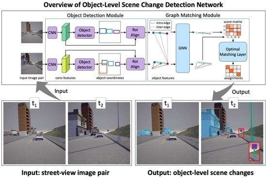
Detecting Object-Level Scene Changes in Images with Viewpoint Differences Using Graph Matching

 ,
,
Abstract
:
1. Introduction
- The proposal of as object-level change detection network that is robust to viewpoint differences, which can be trained using bounding boxes and the correspondences between them;
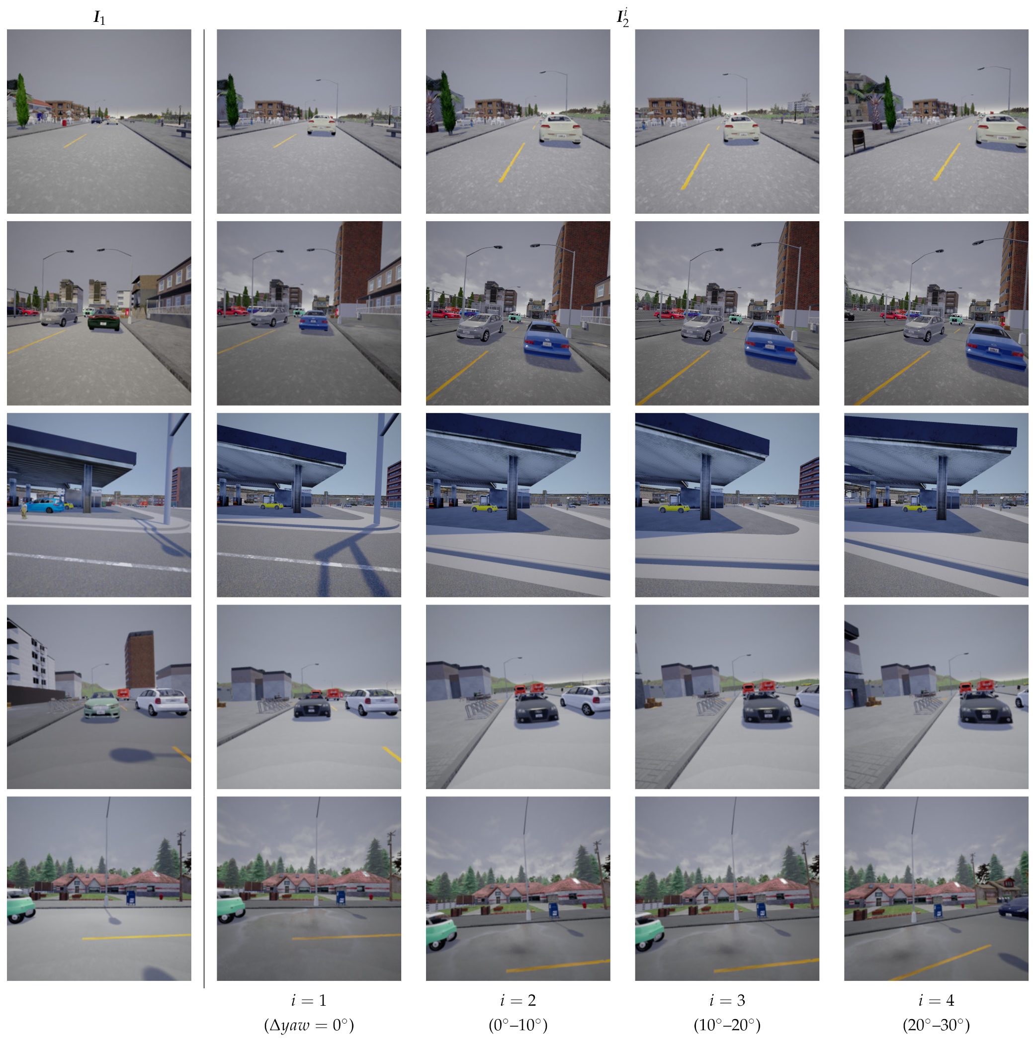
- The development of an SOCD dataset to allow for the study of the performance of object-level change detection methods at different scales of viewpoint differences (the SOCD dataset will be publicly available);
- Experiments on the developed dataset that confirmed that the proposed method outperformed the baseline method in terms of the accuracy of object-level change detection.
2. Related Work
2.1. Image Change Detection
2.2. Graph Matching
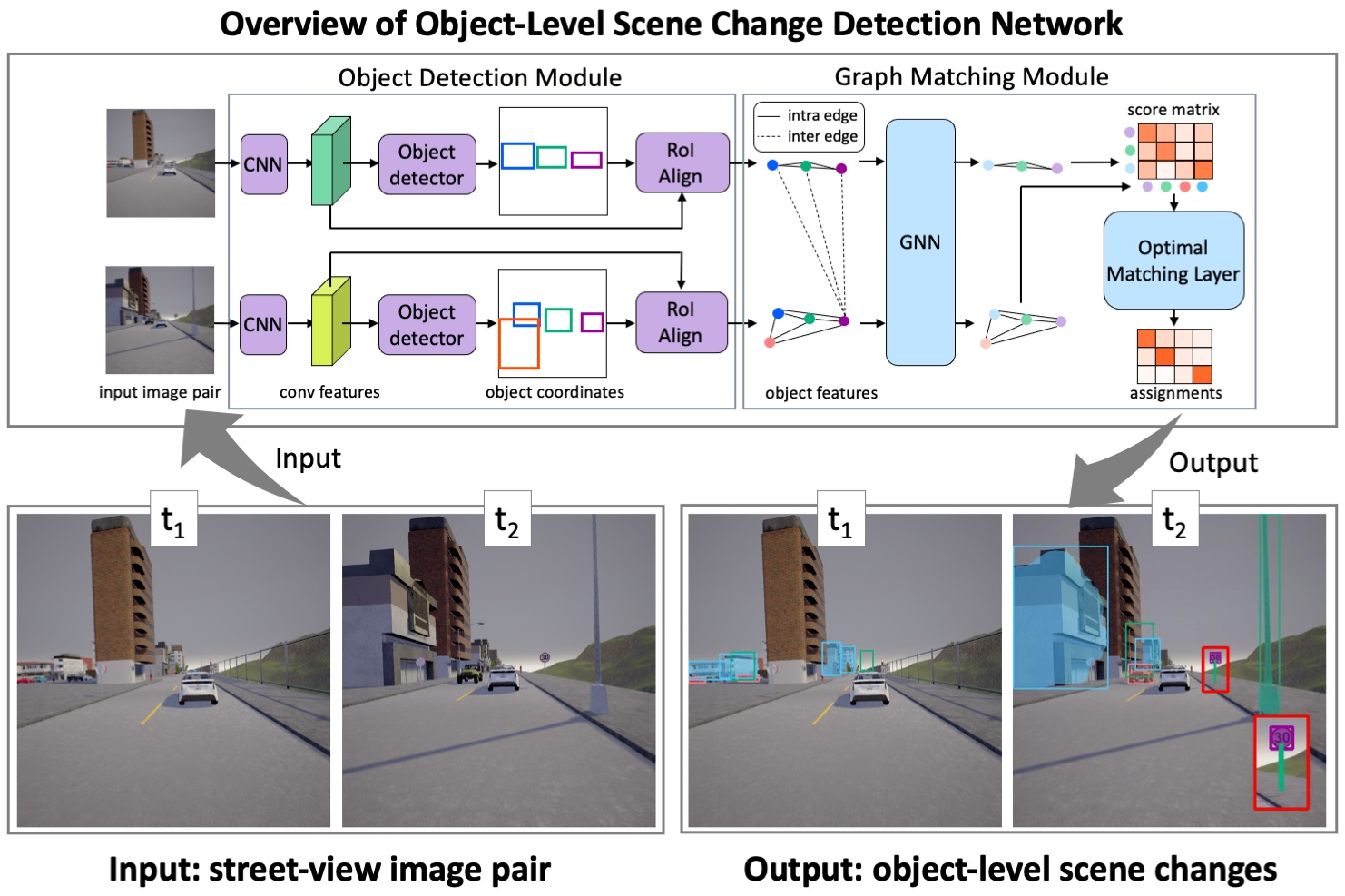
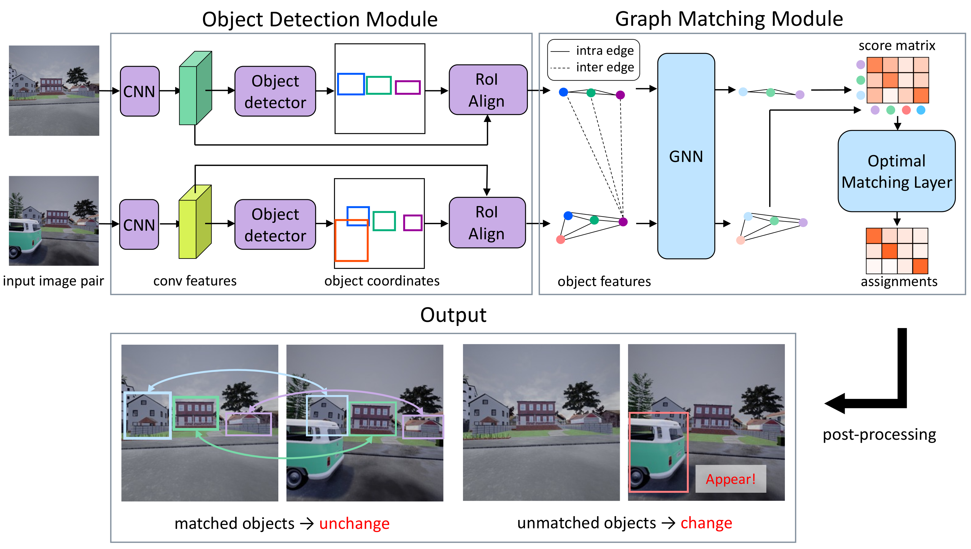
3. Methods
3.1. Formulation
3.2. Object Detection Module
- 1.
- Object Categories, which were sets of labels that described the categories;
- 2.
- Object Region Coordinates, which were sets of vectors that defined the bounding box coordinates of the objects;
- 3.
- Object Features, which were sets of vectors that encoded the visual information and were extracted from each object region using RoIAlign [29] (we used ground truth bounding boxes for training and predicted bounding boxes for testing to extract features);
- 4.
- Object Masks (Optional), which were sets of binary masks of the objects that were provided when we used an instance segmentation network.
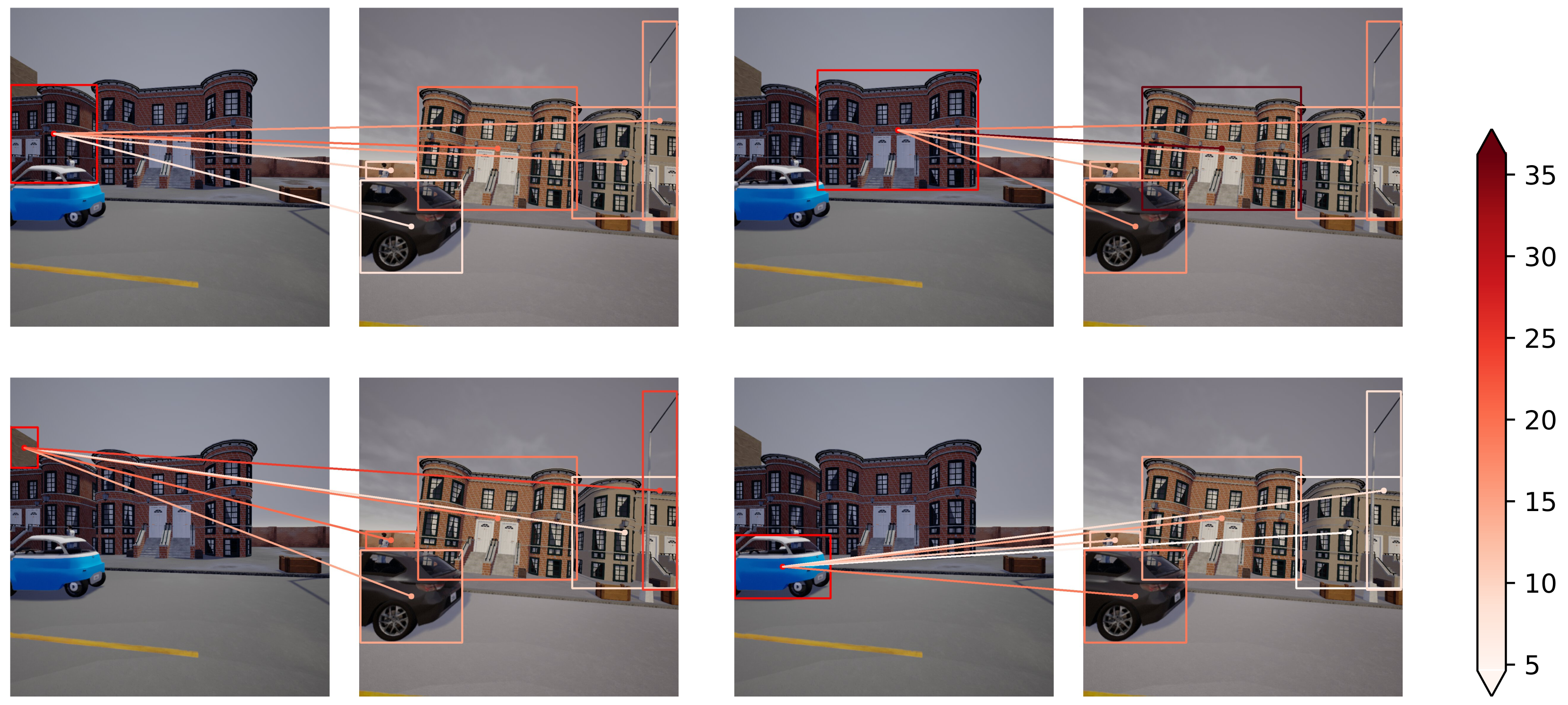
3.3. Graph Matching Module
3.3.1. Feature Refinement
3.3.2. Score Matrix Prediction
3.3.3. Matching Prediction
3.3.4. Post-Processing
3.4. Loss Function
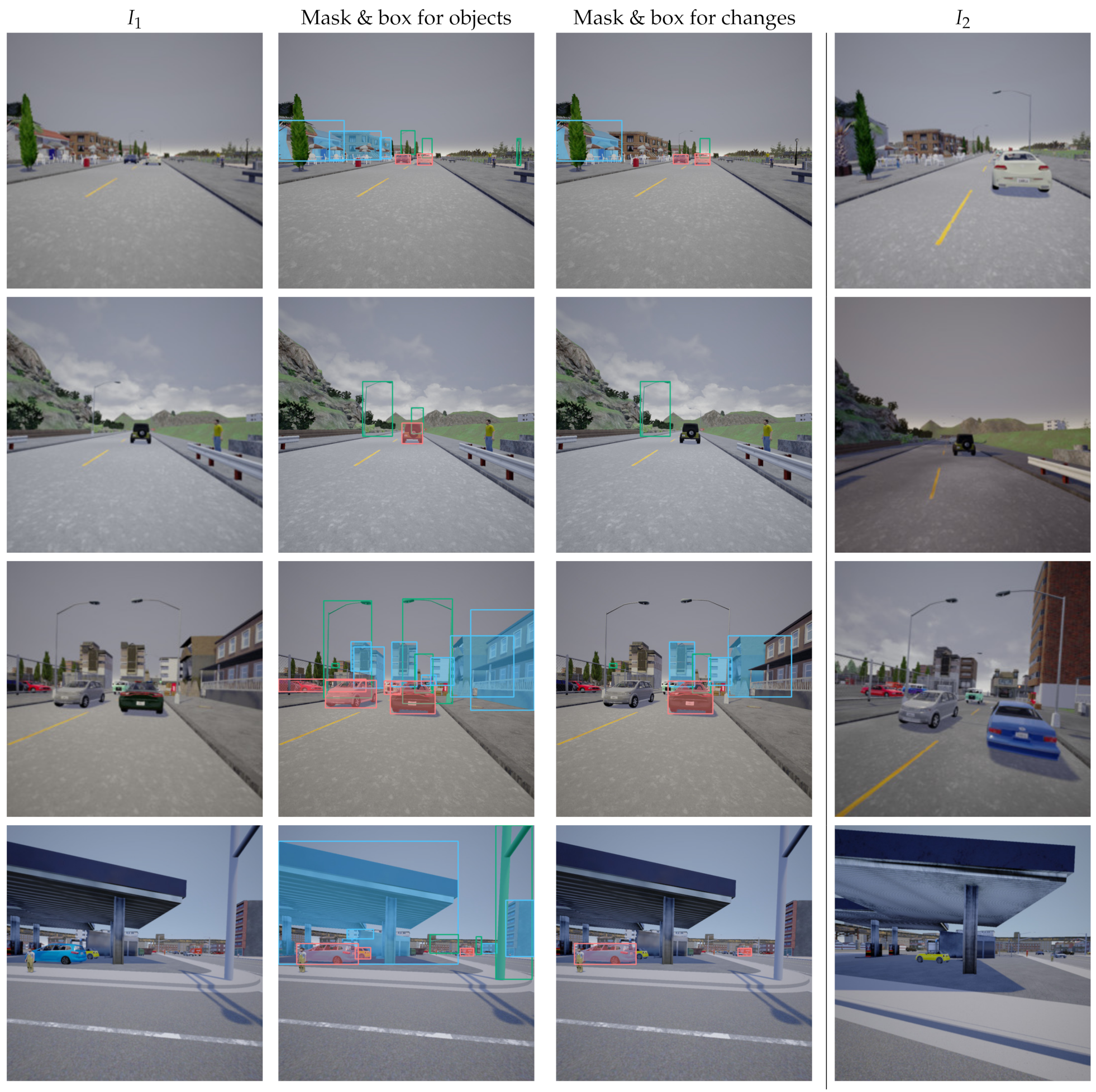
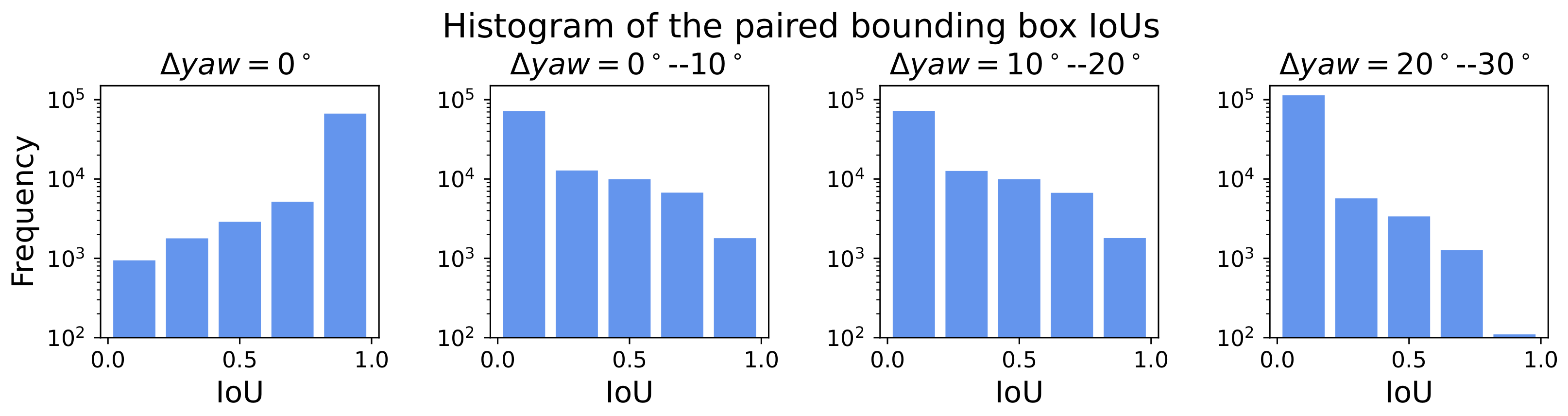
4. Dataset
5. Experiments
5.1. Experimental Settings
5.1.1. Dataset Settings
5.1.2. Implementation Details
5.1.3. Comparison to Other Methods
- 1.
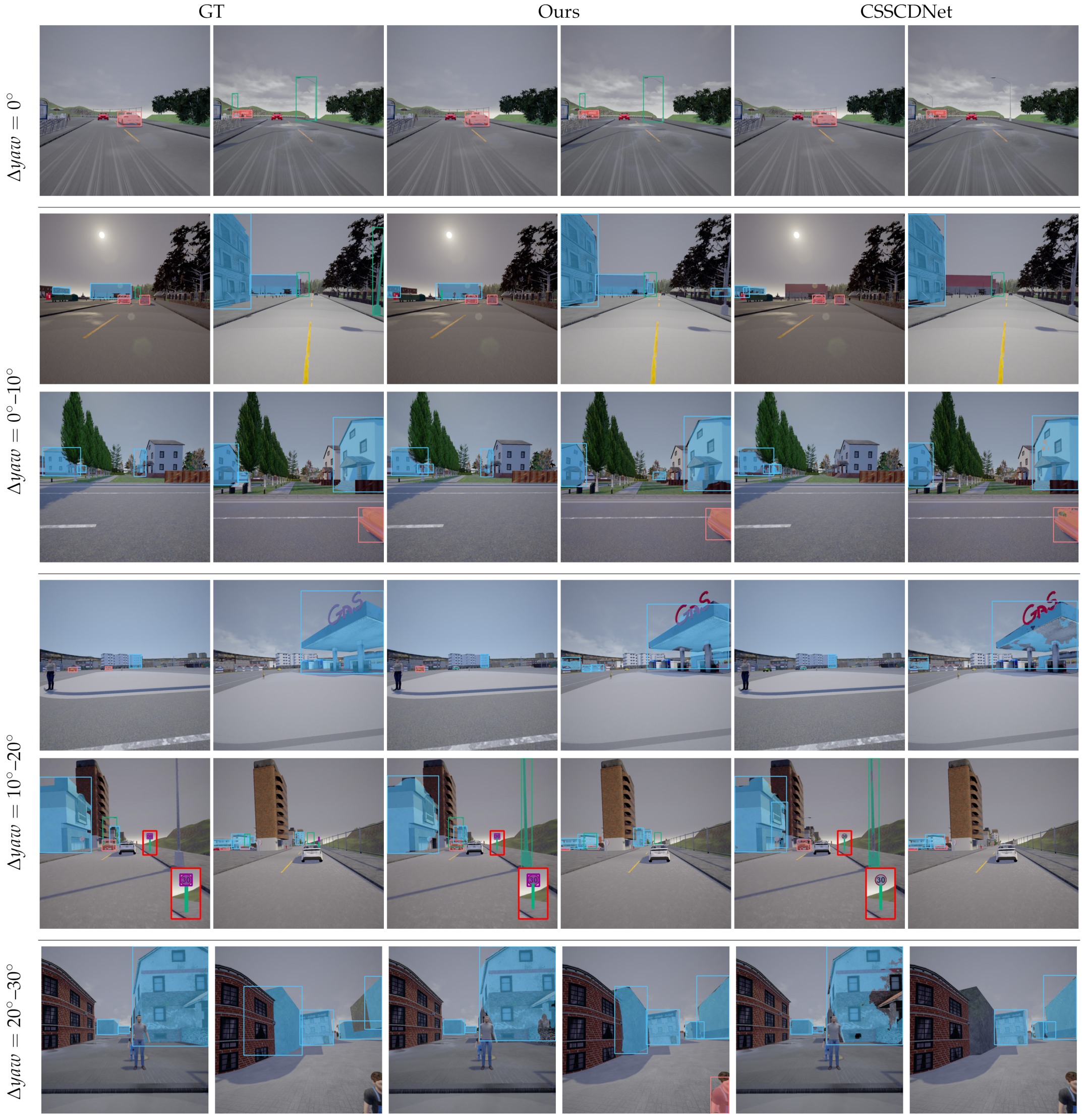
- Pixel-Level Change Detection Methods: Most of the existing methods could not be directly compared to our method because they detected pixel-level changes rather than object-level changes. To compare our method to existing pixel-level change detection networks, we augmented the existing methods by adding post-processing that converted pixel-level change masks into instance masks or bounding boxes. Specifically, the change masks in the existing methods were clipped using the outputs of the pre-trained Mask R-CNN. This clipping was performed when more than 50% of the instance mask overlapped the change mask in the experiment. We used ChangeNet [47] and CSSCDNet [18] as the pixel-level networks;
- 2.
- Our Method Without the Graph Matching Module: A model without the graph matching module was tested using the proposed method. This model created a matrix whose elements were the distances between object features in and and then found matches in post-processing, which was equivalent to that described in Section 3.3.4;
- 3.
- Our Method With a GT Mask: A model that used the correct bounding boxes instead of the bounding boxes that were extracted by the object detector was also tested. We used the same parameters for the feature extractor and the graph matching module as those that were used for the proposed trained network.
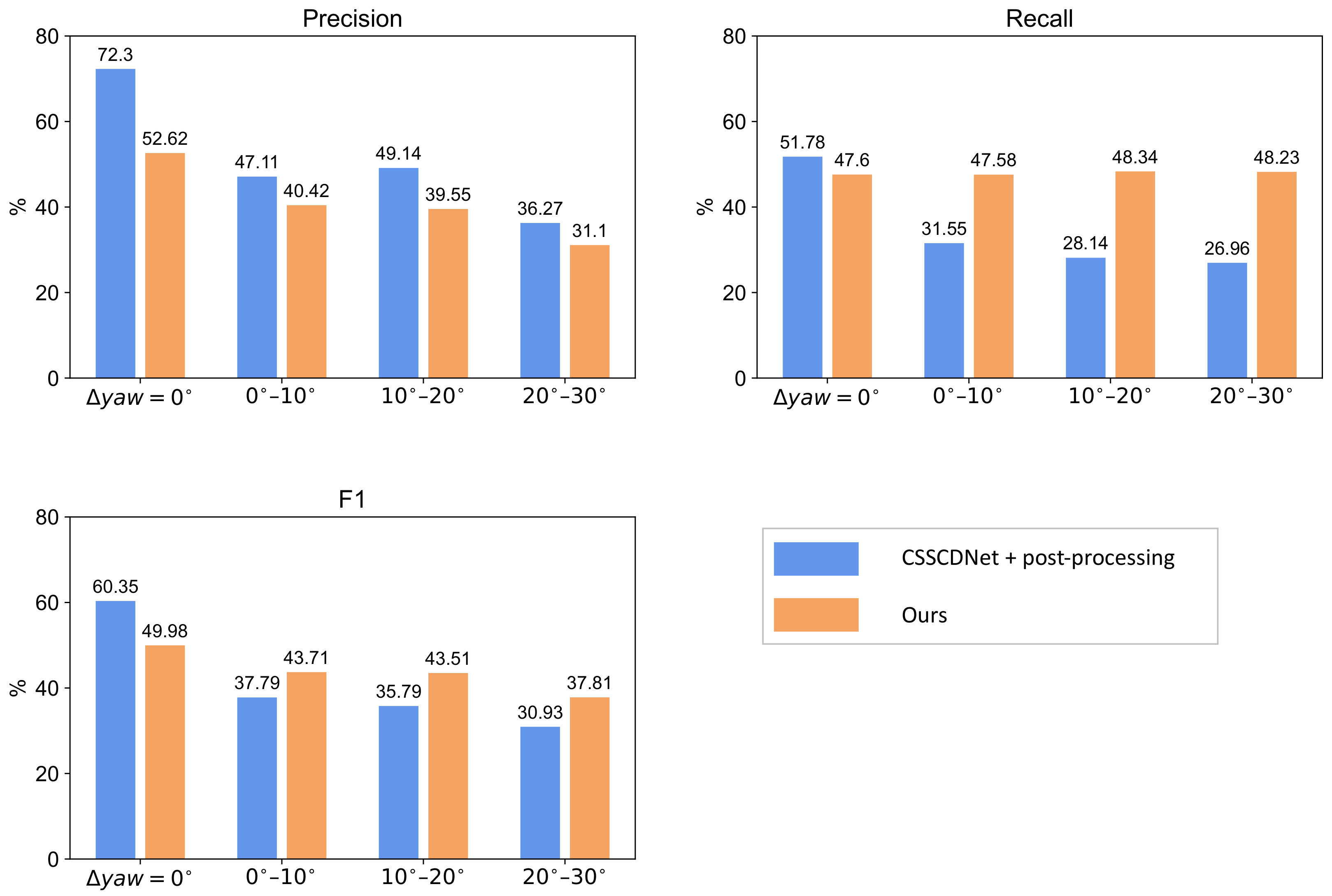
5.1.4. Evaluation Metrics
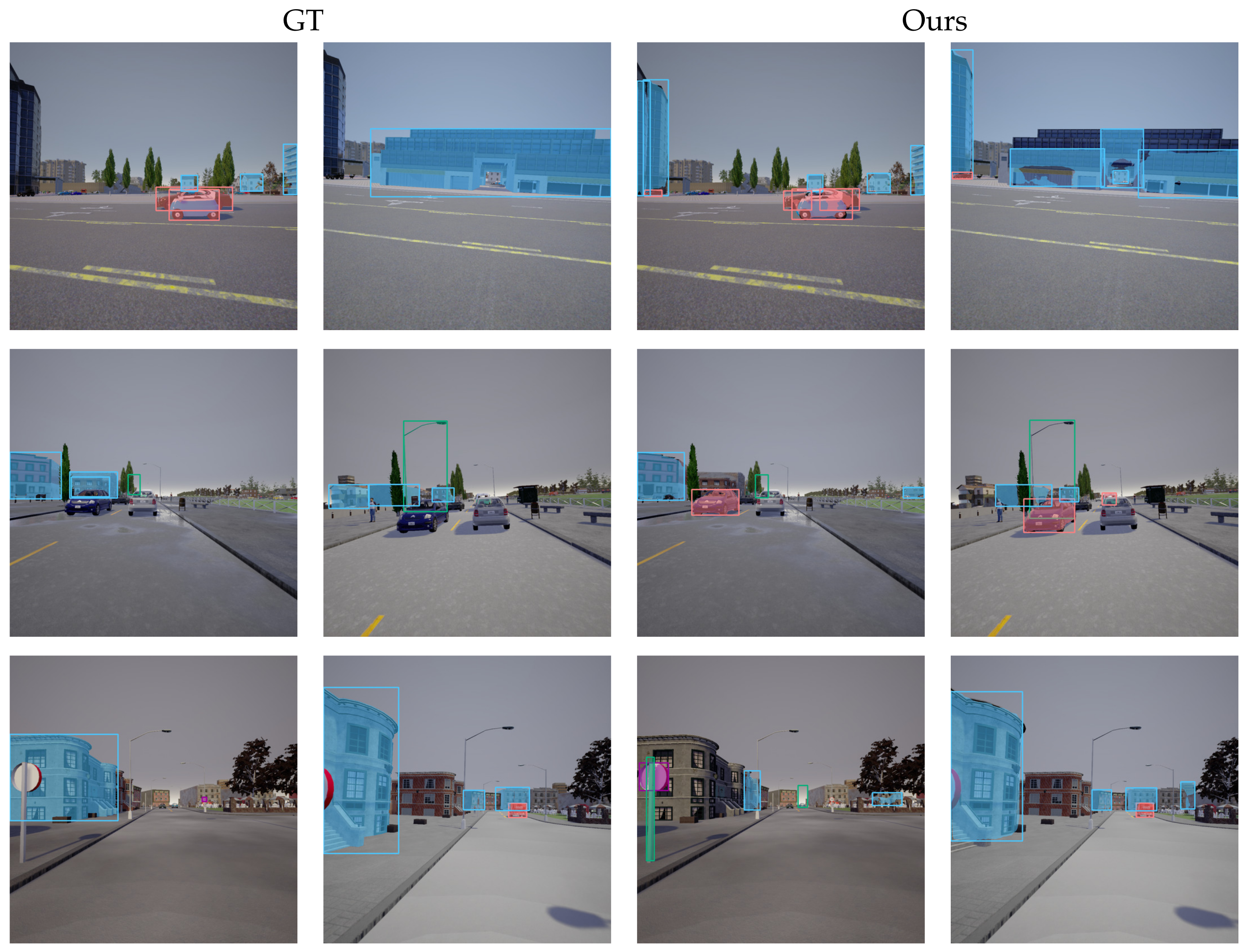
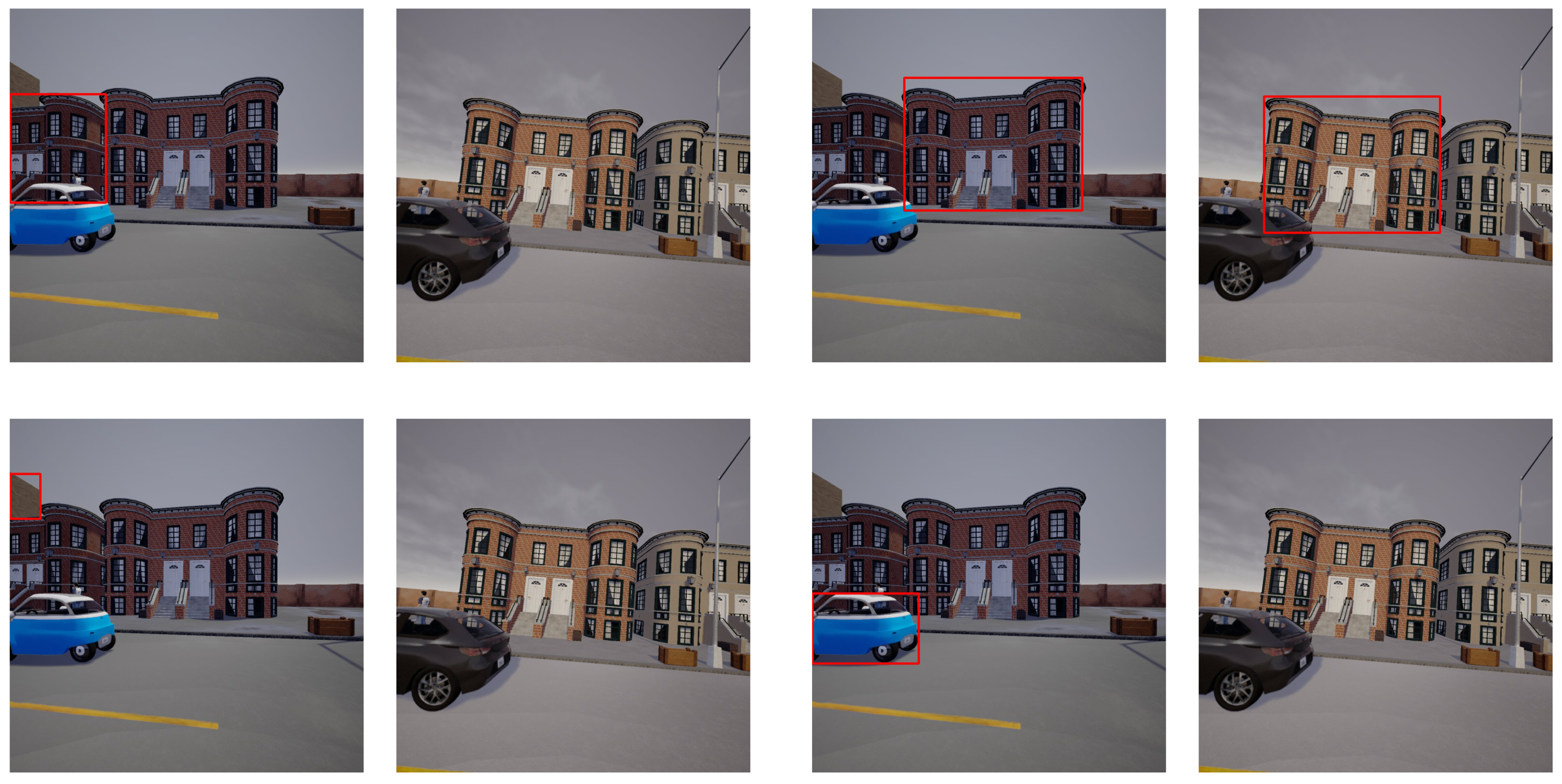
5.2. Experimental Results
6. Discussion
6.1. Comparison to Existing Methods
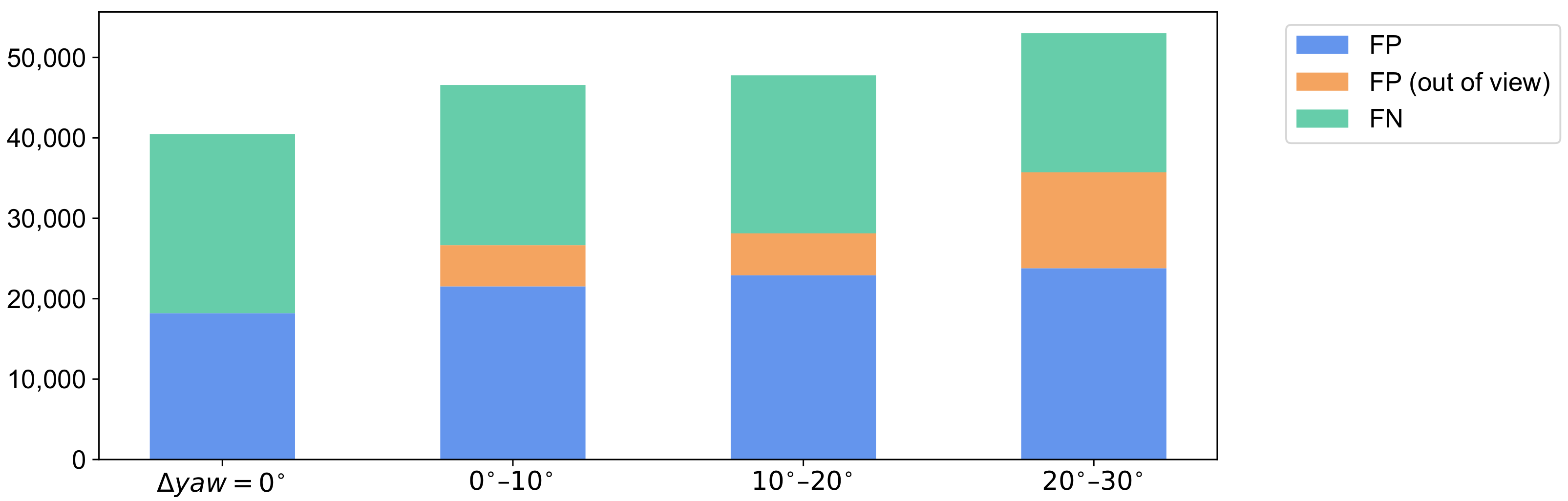
6.2. Error Analysis
6.3. Limitations and Future Directions
7. Conclusions
Author Contributions
Funding
Data Availability Statement
Acknowledgments
Conflicts of Interest
References
- Lu, D.; Mausel, P.; Brondízio, E.; Moran, E. Change detection techniques. Int. J. Remote Sens. 2004, 25, 2365–2401. [Google Scholar] [CrossRef]
- Radke, R.J.; Andra, S.; Al-Kofahi, O.; Roysam, B. Image Change Detection Algorithms: A Systematic Survey. IEEE Trans. Image Process. 2005, 14, 294–307. [Google Scholar] [CrossRef] [PubMed]
- Bai, B.; Fu, W.; Lu, T.; Li, S. Edge-Guided Recurrent Convolutional Neural Network for Multitemporal Remote Sensing Image Building Change Detection. IEEE Trans. Geosci. Remote Sens. 2022, 60, 5610613. [Google Scholar] [CrossRef]
- Wahl, D.E.; Yocky, D.A.; Jakowatz, C.V.; Simonson, K.M. A New Maximum-Likelihood Change Estimator for Two-Pass SAR Coherent Change Detection. IEEE Trans. Geosci. Remote Sens. 2016, 54, 2460–2469. [Google Scholar] [CrossRef]
- Wu, C.; Du, B.; Zhang, L. Slow Feature Analysis for Change Detection in Multispectral Imagery. IEEE Trans. Geosci. Remote Sens. 2014, 52, 2858–2874. [Google Scholar] [CrossRef]
- Liu, S.; Bruzzone, L.; Bovolo, F.; Zanetti, M.; Du, P. Sequential Spectral Change Vector Analysis for Iteratively Discovering and Detecting Multiple Changes in Hyperspectral Images. IEEE Trans. Geosci. Remote Sens. 2015, 53, 4363–4378. [Google Scholar] [CrossRef]
- Hazel, G. Object-level change detection in spectral imagery. IEEE Trans. Geosci. Remote Sens. 2001, 39, 553–561. [Google Scholar] [CrossRef]
- Celik, T. Change Detection in Satellite Images Using a Genetic Algorithm Approach. IEEE Geosci. Remote Sens. Lett. 2010, 7, 386–390. [Google Scholar] [CrossRef]
- Benedek, C.; Sziranyi, T. Change Detection in Optical Aerial Images by a Multilayer Conditional Mixed Markov Model. IEEE Trans. Geosci. Remote Sens. 2009, 47, 3416–3430. [Google Scholar] [CrossRef]
- Chen, B.; Chen, Z.; Deng, L.; Duan, Y.; Zhou, J. Building change detection with RGB-D map generated from UAV images. Neurocomputing 2016, 208, 350–364. [Google Scholar] [CrossRef]
- Feurer, D.; Vinatier, F. Joining multi-epoch archival aerial images in a single SfM block allows 3-D change detection with almost exclusively image information. ISPRS J. Photogramm. Remote Sens. 2018, 146, 495–506. [Google Scholar] [CrossRef]
- Taneja, A.; Ballan, L.; Pollefeys, M. Image Based Detection of Geometric Changes in Urban Environments. In Proceedings of the IEEE International Conference on Computer Vision, Barcelona, Spain, 6–13 November 2011; pp. 2336–2343. [Google Scholar] [CrossRef]
- Alcantarilla, P.F.; Stent, S.; Ros, G.; Arroyo, R.; Gherardi, R. Street-View Change Detection with Deconvolutional Networks. Auton. Robot. 2018, 42, 1301–1322. [Google Scholar] [CrossRef]
- Palazzolo, E.; Stachniss, C. Fast Image-Based Geometric Change Detection Given a 3D Model. In Proceedings of the IEEE International Conference on Robotics and Automation (ICRA), Brisbane, QLD, Australia, 21–26 May 2018; pp. 6308–6315. [Google Scholar] [CrossRef]
- Jo, K.; Kim, C.; Sunwoo, M. Simultaneous Localization and Map Change Update for the High Definition Map-based Autonomous Driving Car. Sensors 2018, 18, 3145. [Google Scholar] [CrossRef] [PubMed]
- Pannen, D.; Liebner, M.; Burgard, W. HD map change detection with a boosted particle filter. In Proceedings of the IEEE International Conference on Robotics and Automation (ICRA), Montreal, QC, Canada, 20–24 May 2019; pp. 2561–2567. [Google Scholar] [CrossRef]
- Furukawa, Y.; Suzuki, K.; Hamaguchi, R.; Onishi, M.; Sakurada, K. Self-supervised Simultaneous Alignment and Change Detection. In Proceedings of the IEEE/RSJ International Conference on Intelligent Robots and Systems (IROS), Las Vegas, NV, USA, 24 October 2020–24 January 2021; pp. 6025–6031. [Google Scholar]
- Sakurada, K.; Shibuya, M.; Wang, W. Weakly Supervised Silhouette-based Semantic Scene Change Detection. In Proceedings of the IEEE International Conference on Robotics and Automation (ICRA), Online, 31 May–31 August 2020; pp. 6861–6867. [Google Scholar]
- Pannen, D.; Liebner, M.; Hempel, W.; Burgard, W. How to Keep HD Maps for Automated Driving Up To Date. In Proceedings of the International Conference on Robotics and Automation (ICRA), online, 31 May–31 August 2020; pp. 2288–2294. [Google Scholar]
- Heo, M.; Kim, J.; Kim, S. HD Map Change Detection with Cross-Domain Deep Metric Learning. In Proceedings of the IEEE/RSJ International Conference on Intelligent Robots and Systems (IROS), Las Vegas, NV, USA, 24 October 2020–24 January 2021; pp. 10218–10224. [Google Scholar]
- Lei, Y.; Peng, D.; Zhang, P.; Ke, Q.; Li, H. Hierarchical Paired Channel Fusion Network for Street Scene Change Detection. IEEE Trans. Image Process. 2020, 30, 55–67. [Google Scholar] [CrossRef]
- Wang, Q.; Zhang, X.; Chen, G.; Dai, F.; Gong, Y.; Zhu, K. Change detection based on Faster R-CNN for high-resolution remote sensing images. Remote Sens. Lett. 2018, 9, 923–932. [Google Scholar] [CrossRef]
- Ji, S.; Shen, Y.; Lu, M.; Zhang, Y. Building Instance Change Detection from Large-Scale Aerial Images using Convolutional Neural Networks and Simulated Samples. Remote Sens. 2019, 11, 1343. [Google Scholar] [CrossRef]
- Zhang, L.; Hu, X.; Zhang, M.; Shu, Z.; Zhou, H. Object-level change detection with a dual correlation attention-guided detector. ISPRS J. Photogramm. Remote Sens. 2021, 177, 147–160. [Google Scholar] [CrossRef]
- Ren, S.; He, K.; Girshick, R.; Sun, J. Faster R-CNN: Towards Real-Time Object Detection with Region Proposal Networks. In Proceedings of the Advances in Neural Information Processing Systems 28, Montreal, QC, Canada, 7–10 September 2015; pp. 91–99. [Google Scholar]
- Dosovitskiy, A.; Ros, G.; Codevilla, F.; Lopez, A.; Koltun, V. CARLA: An Open Urban Driving Simulator. In Proceedings of the 1st Annual Conference on Robot Learning, Mountain View, CA, USA, 13–15 November 2017; Volume 78, pp. 1–16. [Google Scholar]
- Sakurada, K.; Okatani, T. Change Detection from a Street Image Pair using CNN Features and Superpixel Segmentation. In Proceedings of the British Machine Vision Conference (BMVC), Swansea, UK, 7–10 September 2015; pp. 61.1–61.12. [Google Scholar] [CrossRef]
- Guo, E.; Fu, X.; Zhu, J.; Deng, M.; Liu, Y.; Zhu, Q.; Li, H. Learning to Measure Changes: Fully Convolutional Siamese Metric Networks for Scene Change Detection. arXiv 2018, arXiv:1810.09111. [Google Scholar]
- He, K.; Gkioxari, G.; Dollár, P.; Girshick, R. Mask R-CNN. In Proceedings of the IEEE International Conference on Computer Vision (ICCV), Venice, Italy, 22–29 October 2017. [Google Scholar]
- Conte, D.; Sansone, C.; Vento, M.; Conte, D.; Foggia, P.; Sansone, C.; Vento, M. Thirty Years Of Graph Matching In Pattern Recognition. Int. J. Pattern Recognit. Artif. Intell. 2004, 18, 265–298. [Google Scholar] [CrossRef]
- Yan, J.; Yang, S.; Hancock, E. Learning for Graph Matching and Related Combinatorial Optimization Problems. In Proceedings of the Twenty-Ninth International Joint Conference on Artificial Intelligence, Yokohama, Japan, 7–15 January 2020; pp. 4988–4996. [Google Scholar] [CrossRef]
- Zanfir, A.; Sminchisescu, C. Deep Learning for Graph Matching. In Proceedings of the IEEE Computer Society Conference on Computer Vision and Pattern Recognition (CVPR), Salt Lake City, UT, USA, 18–22 June 2018; pp. 2684–2693. [Google Scholar]
- Wang, R.; Yan, J.; Yang, X. Learning Combinatorial Embedding Networks for Deep Graph Matching. In Proceedings of the IEEE International Conference on Computer Vision (ICCV), Seoul, Korea, 27 October–2 November 2019. [Google Scholar]
- Sarlin, P.E.; Detone, D.; Malisiewicz, T.; Rabinovich, A.; Zurich, E. SuperGlue: Learning Feature Matching with Graph Neural Networks. In Proceedings of the EEE/CVF Conference on Computer Vision and Pattern Recognition (CVPR), Online, 14–19 June 2020; pp. 4938–4947. [Google Scholar]
- Battaglia, P.W.; Hamrick, J.B.; Bapst, V.; Sanchez-Gonzalez, A.; Zambaldi, V.; Malinowski, M.; Tacchetti, A.; Raposo, D.; Santoro, A.; Faulkner, R.; et al. Relational inductive biases, deep learning, and graph networks. arXiv 2018, arXiv:1806.01261. [Google Scholar]
- Gilmer, J.; Schoenholz, S.S.; Riley, P.F.; Vinyals, O.; Dahl, G.E. Neural Message Passing for Quantum Chemistry. In Proceedings of the International Conference on Machine Learning (ICML), Sydney, NSW, Australia, 6–11 August 2017; pp. 1263–1272. [Google Scholar]
- Cuturi, M. Sinkhorn Distances: Lightspeed Computation of Optimal Transport. In Proceedings of the Advances in Neural Information Processing Systems, Lake Tahoe, NV, USA, 5–10 December 2013; Volume 26, pp. 2292–2300. [Google Scholar]
- Sinkhorn, R.; Knopp, P. Concerning Nonnegative Matrices and Doubly Stochastic Matrices. Pac. J. Math. 1967, 21, 343–348. [Google Scholar] [CrossRef]
- Duan, K.; Bai, S.; Xie, L.; Qi, H.; Huang, Q.; Tian, Q. CenterNet: Keypoint Triplets for Object Detection. In Proceedings of the IEEE/CVF International Conference on Computer Vision (ICCV), Seoul, Korea, 27 October–2 November 2019. [Google Scholar]
- Carion, N.; Massa, F.; Synnaeve, G.; Usunier, N.; Kirillov, A.; Zagoruyko, S. End-to-End Object Detection with Transformers. In Proceedings of the 16th European Conference, Glasgow, UK, 23–28 August 2020; pp. 213–229. [Google Scholar]
- Wang, C.Y.; Bochkovskiy, A.; Liao, H.Y.M. Scaled-YOLOv4: Scaling Cross Stage Partial Network. In Proceedings of the IEEE/CVF Conference on Computer Vision and Pattern Recognition (CVPR), Online, 19–25 June 2021; pp. 13029–13038. [Google Scholar]
- Dai, X.; Chen, Y.; Xiao, B.; Chen, D.; Liu, M.; Yuan, L.; Zhang, L. Dynamic Head: Unifying Object Detection Heads with Attentions. In Proceedings of the IEEE/CVF Conference on Computer Vision and Pattern Recognition (CVPR), Online, 19–25 June 2021. [Google Scholar]
- Vaswani, A.; Shazeer, N.; Parmar, N.; Uszkoreit, J.; Jones, L.; Gomez, A.N.; Kaiser, L.U.; Polosukhin, I. Attention is All you Need. In Proceedings of the Advances in Neural Information Processing Systems, Long Beach, CA, USA, 4–9 December 2017; Volume 30. [Google Scholar]
- Wang, Y.; Jodoin, P.M.; Porikli, F.; Konrad, J.; Benezeth, Y.; Ishwar, P. CDnet 2014: An Expanded Change Detection Benchmark Dataset. In Proceedings of the IEEE Conference on Computer Vision and Pattern Recognition (CVPR) Workshops, Columbus, OH, USA, 23–28 June 2014; pp. 387–394. [Google Scholar]
- Lin, T.Y.; Dollár, P.; Girshick, R.; He, K.; Hariharan, B.; Belongie, S. Feature pyramid networks for object detection. In Proceedings of the IEEE Conference on Computer Vision and Pattern Recognition (CVPR), Honolulu, HI, USA, 21–26 July 2017; pp. 2117–2125. [Google Scholar] [CrossRef]
- He, K.; Zhang, X.; Ren, S.; Sun, J. Deep Residual Learning for Image Recognition. In Proceedings of the IEEE Conference on Computer Vision and Pattern Recognition (CVPR), Las Vegas, NV, USA, 27–30 June 2016; pp. 770–778. [Google Scholar] [CrossRef]
- Varghese, A.; Gubbi, J.; Ramaswamy, A. ChangeNet: A Deep Learning Architecture for Visual Change Detection. In Proceedings of the ECCV Workshop, Munich, Germany, 8–14 September 2018. [Google Scholar]
- Minaee, S.; Boykov, Y.; Porikli, F.; Plaza, A.; Kehtarnavaz, N.; Terzopoulos, D. Image Segmentation Using Deep Learning: A Survey. IEEE Trans. Pattern Anal. Mach. Intell. 2022, 44, 3523–3542. [Google Scholar] [CrossRef] [PubMed]
- Garcia-Garcia, A.; Orts-Escolano, S.; Oprea, S.; Villena-Martinez, V.; Garcia-Rodriguez, J. A Review on Deep Learning Techniques Applied to Semantic Segmentation. arXiv 2017, arXiv:1704.06857. [Google Scholar]
- Kirillov, A.; He, K.; Girshick, R.; Rother, C.; Dollar, P. Panoptic Segmentation. In Proceedings of the IEEE/CVF Conference on Computer Vision and Pattern Recognition (CVPR), Long Beach, CA, USA, 15–20 June 2019. [Google Scholar]
- Cheng, B.; Collins, M.D.; Zhu, Y.; Liu, T.; Huang, T.S.; Adam, H.; Chen, L.C. Panoptic-DeepLab: A Simple, Strong, and Fast Baseline for Bottom-Up Panoptic Segmentation. In Proceedings of the IEEE/CVF Conference on Computer Vision and Pattern Recognition (CVPR), Online, 13–19 June 2020. [Google Scholar]
- Li, Y.; Zhao, H.; Qi, X.; Wang, L.; Li, Z.; Sun, J.; Jia, J. Fully Convolutional Networks for Panoptic Segmentation. In Proceedings of the IEEE/CVF Conference on Computer Vision and Pattern Recognition (CVPR), Online, 20–25 June 2021; pp. 214–223. [Google Scholar]
- Wang, H.; Zhu, Y.; Adam, H.; Yuille, A.; Chen, L.C. MaX-DeepLab: End-to-End Panoptic Segmentation With Mask Transformers. In Proceedings of the IEEE/CVF Conference on Computer Vision and Pattern Recognition (CVPR), Online, 20–25 June 2021; pp. 5463–5474. [Google Scholar]
- Li, Z.; Wang, W.; Xie, E.; Yu, Z.; Anandkumar, A.; Alvarez, J.M.; Luo, P.; Lu, T. Panoptic SegFormer: Delving Deeper Into Panoptic Segmentation With Transformers. In Proceedings of the IEEE/CVF Conference on Computer Vision and Pattern Recognition (CVPR), New Orleans, LA, USA, 19–24 June 2022; pp. 1280–1289. [Google Scholar]
- Vinyals, O.; Toshev, A.; Bengio, S.; Erhan, D. Show and tell: A neural image caption generator. In Proceedings of the IEEE/CVF Conference on Computer Vision and Pattern Recognition (CVPR), Boston, MA, USA, 7–12 June 2015; pp. 3156–3164. [Google Scholar]
- Xu, K.; Ba, J.; Kiros, R.; Cho, K.; Courville, A.; Salakhudinov, R.; Zemel, R.; Bengio, Y. Show, Attend and Tell: Neural Image Caption Generation with Visual Attention. In Proceedings of the 32nd International Conference on Machine Learning, Lille, France, 6–11 July 2015; Volume 37, pp. 2048–2057. [Google Scholar]
- Anderson, P.; He, X.; Buehler, C.; Teney, D.; Johnson, M.; Gould, S.; Zhang, L. Bottom-Up and Top-Down Attention for Image Captioning and Visual Question Answering. In Proceedings of the IEEE Conference on Computer Vision and Pattern Recognition (CVPR), Salt Lake City, UT, USA, 18–23 June 2018. [Google Scholar]
- Jhamtani, H.; Berg-Kirkpatrick, T. Learning to Describe Differences Between Pairs of Similar Images. In Proceedings of the 2018 Conference on Empirical Methods in Natural Language Processing, Brussels, Belgium, 31 October–4 November 2018; pp. 4024–4034. [Google Scholar] [CrossRef] [Green Version]
- Park, D.H.; Darrell, T.; Rohrbach, A. Robust Change Captioning. In Proceedings of the IEEE International Conference on Computer Vision (ICCV), Seoul, Korea, 27 October–2 November 2019; pp. 4624–4633. [Google Scholar]
- Qiu, Y.; Yamamoto, S.; Nakashima, K.; Suzuki, R.; Iwata, K.; Kataoka, H.; Satoh, Y. Describing and Localizing Multiple Changes With Transformers. In Proceedings of the IEEE/CVF International Conference on Computer Vision (ICCV), Online, 11–17 October 2021; pp. 1971–1980. [Google Scholar]


| Dataset | Domain | Image Type | Viewpoint Difference | Number of Pairs | Number of Semantic Classes | Annotation | |
|---|---|---|---|---|---|---|---|
| Pixel-Level | Object-Level | ||||||
| PCD (TSUNAMI) [27] | Real | Panoramic | Small | 100 | - * | 🗸 | |
| PCD (GSV) [27] | Real | Panoramic | Small | 100 | - * | 🗸 | |
| VL-CMU-CD [13] | Real | Perspective | Small | 1362 | - * | 🗸 | |
| CDnet2014 [44] | Real | Perspective | None | 70,000 | - * | 🗸 | |
| SOCD (Ours) | Synthetic | Perspective | None∼Large (Four different viewpoint scales) | 15,000 | 4 | 🗸 | 🗸 |
| Method | Viewpoint Difference | |||
|---|---|---|---|---|
| – | – | – | ||
| Pixel-level Methods + Post-Processing | ||||
| ChangeNet [47] | 0.219 | 0.142 | 0.155 | 0.133 |
| CSSCDNet [18] (Without correction layer) | 0.453 | 0.234 | 0.241 | 0.205 |
| CSSCDNet [18] (With correction layer) | 0.508 | 0.274 | 0.258 | 0.208 |
| Object-level Methods | ||||
| Ours (Without graph matching module) | 0.406 | 0.337 | 0.335 | 0.295 |
| Ours | 0.463 | 0.401 | 0.396 | 0.354 |
| Ours (With GT mask) | 0.852 | 0.650 | 0.652 | 0.546 |
Publisher’s Note: MDPI stays neutral with regard to jurisdictional claims in published maps and institutional affiliations. |
© 2022 by the authors. Licensee MDPI, Basel, Switzerland. This article is an open access article distributed under the terms and conditions of the Creative Commons Attribution (CC BY) license (https://creativecommons.org/licenses/by/4.0/).
Share and Cite
Doi, K.; Hamaguchi, R.; Iwasawa, Y.; Onishi, M.; Matsuo, Y.; Sakurada, K. Detecting Object-Level Scene Changes in Images with Viewpoint Differences Using Graph Matching. Remote Sens. 2022, 14, 4225. https://doi.org/10.3390/rs14174225
Doi K, Hamaguchi R, Iwasawa Y, Onishi M, Matsuo Y, Sakurada K. Detecting Object-Level Scene Changes in Images with Viewpoint Differences Using Graph Matching. Remote Sensing. 2022; 14(17):4225. https://doi.org/10.3390/rs14174225
Chicago/Turabian StyleDoi, Kento, Ryuhei Hamaguchi, Yusuke Iwasawa, Masaki Onishi, Yutaka Matsuo, and Ken Sakurada. 2022. "Detecting Object-Level Scene Changes in Images with Viewpoint Differences Using Graph Matching" Remote Sensing 14, no. 17: 4225. https://doi.org/10.3390/rs14174225
APA StyleDoi, K., Hamaguchi, R., Iwasawa, Y., Onishi, M., Matsuo, Y., & Sakurada, K. (2022). Detecting Object-Level Scene Changes in Images with Viewpoint Differences Using Graph Matching. Remote Sensing, 14(17), 4225. https://doi.org/10.3390/rs14174225