Abstract
A balanced dataset is generally beneficial to underwater acoustic target recognition. However, the imbalanced class distribution is always meted out in a real scene. To address this, a weighted cross entropy loss function based on trigonometric function is proposed. Then, the proposed loss function is applied in a multi-scale residual convolutional neural network (named MR-CNN-A network) embedded with an attention mechanism for the recognition task. Firstly, a multi-scale convolution kernel is used to obtain multi-scale features. Then, an attention mechanism is used to fuse these multi-scale feature maps. Furthermore, a cosx-function-weighted cross-entropy loss function is used to deal with the class imbalance in underwater acoustic data. This function adjusts the loss ratio of each sample by adjusting the loss interval of every mini-batch based on cosx term to achieve a balanced total loss for each class. Two imbalanced underwater acoustic data sets, ShipsEar and autonomous underwater vehicle (self-collected data) are used to evaluate the proposed network. The experimental results show that the proposed network outperforms the support vector machine and a simple convolutional neural network. Compared with the other three loss functions, the proposed loss function achieves better stability and adaptability. The results strongly demonstrate the validity of the proposed loss function and the network.
1. Introduction
The underwater acoustic target recognition is an information processing technology that uses the data obtained by passive or active sonar to distinguish the target type in these data. Its key point is the target feature extraction. Underwater acoustic target recognition is a challenging research direction on underwater acoustic signal processing, which serves as a key technology in various marine applications, such as information acquisition, ocean surveillance, ocean resource exploration, etc. [1,2].
The existing recognition methods consist of two main groups: Traditional recognition methods and deep-learning-based methods. Traditional recognition methods are currently used routinely. Its core lies in the hand-crafted feature extraction and classifier design [3,4,5]. For example, Su [3] adopted LOFAR spectrum, bi-spectrum, and other features to achieve a better classification of underwater acoustic targets. However, the hand-crafted feature extraction largely depends on the experience of the designer, so its scope of application is limited. In contrast, the deep-learning-based recognition method is data-driven, does not rely on any prior information, and has good generalization. Compared with the hand-crafted feature, the feature learned by deep network contains higher-order items and achieves implicit relationships, which can better express the information of the target. As a result, the deep-learning-based recognition method has become a hot research topic.
For deep learning method research, a balanced and large underwater acoustic dataset is needed. However, the underwater acoustic dataset is often imbalanced, which is not helpful for the research. In other words, the occurrence frequency of some classes in an underwater acoustic dataset is high, while the occurrence frequency of some other classes is low, which leads to the objective problem of imbalanced classification. Therefore, when using deep learning methods for recognition, the recognition results tend to be skewed toward the larger categories of targets.
At present, the application of deep learning in underwater acoustic target recognition is not particularly extensive, especially the research on imbalanced targets is scarce [6,7,8,9]. Considering the complex marine environment, Li et al. [6] proposed a bi-Long Short-Term Memory (bi-LSTM) network for underwater acoustic target recognition, which can learn the temporal correlation of acoustic signals. Ferguson et al. [7] realized a Convolutional Neural Network (CNN) on cepstrum data and achieved a high recognition rate. To address the problem that line spectrum is not accurate enough for deep learning under low SNR, Yang et al. [8] proposed an improved bicoherence spectrum and applied it to three deep belief networks. The experimental results show that the proposed bicoherence spectrum is more suitable for deep learning method than the traditional spectrum. Wu et al. [9] converted signal into a time-frequency image (such as LOFAR) and entered it into CNN to achieve feature extraction and classification of ships, which also achieved a high recognition accuracy. All these works demonstrate that deep learning can be applied in underwater acoustic target recognition tasks and can achieve noticeable progress.
The imbalance of datasets is a common problem in many fields, including speech and computer vision [10,11,12]. Moreover, several attempts have already taken place in the field of underwater acoustic target recognition.
The solutions for imbalanced data fall into two main categories: Rebalancing on the data level and rebalancing on the algorithm level. Rebalancing on data level means changing the data distribution using over-sampling and under-sampling. The use of over-sampling on the data with low distribution density and under-sampling on the data with high distribution density makes the distribution of data to be balanced [13,14]. With balanced data, the accuracy improvement is obvious. However, this data rebalancing method has obvious drawbacks, such as under-sampling, which can discard potentially useful data.
On the other hand, rebalancing on the algorithm level means adjusting the training or reasoning algorithms to resist the effect of data imbalance with the same training dataset. A typical way to rebalance on the algorithm level is to optimize the loss function with the weight of each class according to the number of samples. For example, Huang et al. [15] proposed a quintuple-based Large Margin Local Embedding-KNN (LMLE-KNN) algorithm to enhance the edges between clusters and outside clusters so that local margin can be easily enforced to reduce any local class imbalance. Huang et al. [16] proposed a new Cluster-based Large Margin Local Embedding (CLMLE) method based on LMLE and an in-cluster loss function in accordance with CLMLE to solve the imbalance. Another way is to design a new loss function to resist the disequilibrium. Dong et al. [10] proposed a loss function named Exponentially Weighted Cross-Entropy Loss (EWCEL) to solve the imbalance in the underwater acoustic target recognition task. EWCEL is achieved by adding an exponential weight influence factor to the standard cross entropy loss. The recognition accuracy achieved by EWCEL is higher than Focal Loss [12] in the underwater acoustic dataset with imbalanced targets and communication signals. Li et al. [17] considered the imbalance problem from the perspective of gradient. Therefore, a new gradient harmonizing mechanism (GHM) was proposed, and two loss functions, GHM-C and GHM-R equilibrium gradient flows were designed for classification and optimization. Lin et al. [12] added a factor to the original cross-entropy loss to reduce the loss of easily classified samples, while it pays more attention to difficult and misclassified samples. After that, a higher recognition accuracy with the help of the new loss function is obtained.
To address the imbalance and poor robustness, two strategies are proposed to learn distinguishing features. On the one side, the attention mechanism is used to fuse the learned multi-scale features. The fusion module based on the attention mechanism is used to highlight the dominant features to suppress high-intensity noise. On the other side, a trigonometric function weighted cross entropy loss function (CFWCEL) is designed to deal with imbalanced data. Finally, a multi-scale residual-convolutional neural network with an embedded attention mechanism (named MR-CNN-A) and CFWCEL is proposed for target recognition. CFWCEL adds an impact factor to the standard cross entropy loss according to the predicted probability of each sample. Different from EWCEL [10] and Focal Loss [12], the CFWCEL decreases faster for negative examples and more gently for positive examples. It is conducive to the convergence of imbalanced data.
The rest of this paper is organized as follows. Section 2 introduces the underwater acoustic target recognition system based on MR-CNN-A. The results of the recognition experiments and the imbalanced experiments are introduced and discussed in Section 3. Finally, the conclusion is presented in Section 4.
2. Materials and Methods
Figure 1 shows the proposed whole recognition system framework. All the data used in this paper are acquired by a passive sonar. After obtaining the acoustic data, several features are obtained, like Mel-Frequency Cepstral Coefficients (MFCC) [18,19,20], which have a natural anti-low frequency noise performance and can suppress underwater acoustic noise to highlight the target information. Then, the MR-CNN-A network is used to realize the extraction and fusion of a multi-scale feature using a multi-scale network and attention mechanism. After that, the CFWCEL is used to realize the insensitivity to imbalanced data. Finally, the fully connected layer with softmax is used as the classifier layer to obtain the predicted category label.

Figure 1.
The recognition system framework.
As shown in Figure 1, the whole recognition framework involves MFCC feature extraction, deep-network-based feature learning, and loss function optimization. The three parts are described in detail in the following parts.
2.1. Feature Preparing
After the signal acquisition, we should prepare several features used as the input of the deep network. In this part, we introduce three different features, like Mel-Frequency Cepstral Coefficients (MFCC) [18,19,20], Hilbert-Huang Transform (HHT) [21], and Detection of Envelope Modulation On Noise (DEMON) [22].
MFCC can be simply understood as an energy-based feature that processes the original acoustic signal approximately as the convolution of a function. Mel is a frequency scale unit of tones, namely Mel frequency, which represents a nonlinear feature of human ears. Moreover, MFCC can be obtained by changing the time domain to the frequency domain and carrying out nonlinear transformation to realize deconvolution. The realization process of MFCC is not elaborated, which can be referred to in references [18,19,20].
HHT is a new time-frequency analysis method that adaptively separates time-frequency signals of different scales by Empirical Mode Decomposition (EMD) [21]. It is no longer limited by the basis function of previous signal analysis methods, and it is a practical tool for processing non-stationary signals, such as water acoustic signals. HHT is mainly composed of EMD and Hilbert Spectrum Analysis (HSA). EMD is adaptively driven by data. It uses signal local pole distribution characteristics to extract characteristic wave functions, which is a set of decomposition functions—Intrinsic Mode Function (IMF) components. IMF can introduce the components of different frequency scales. In other words, it is possible to adaptively separate the fluctuations or trends of different scales in the signal and then obtain a group of quantities that characterize the time-frequency distribution of the entire signal. This feature has better recognizability.
Modulation-spectrum-based DEMON is a traditional spectrum, which shows a clear physical meaning [22]. Moreover, DEMON represents the structure of a ship propeller. DEMON is obtained from the modulation phenomenon of ship radiated noise when the propeller rotates at different speeds in water. In other words, the amplitude of radiated noise fluctuates with the change of acquisition time, therefore, the modulation envelope can be extracted from the time waveform of ship radiated noise. Generally, there are three demodulation methods, square low pass filter demodulation, absolute low pass filter demodulation, and Hilbert filter demodulation. The square low-pass filter demodulation method is used in our experiments.
2.2. MR-CNN-A Network
2.2.1. Attention Mechanism Based Multi-Scale Feature Fusion
Generally speaking, smaller-scale samples pay more attention to the overall outline, while higher-scale samples pay more attention to the details of the target. With the fusion of different scales of samples, more details of the target can be obtained. Consequently, a multi-scale feature learning and fusion block are used in the proposed network. To obtain the multi-scale feature, several convolutional kernels with different sizes are used as the different scalers in which the size of convolutional kernel represents the scale size in different channels. After feature extraction in each channel, an attention mechanism is used to fuse the features in different channels. Figure 2 provides the attention-mechanism-based feature fusion framework. Attention-mechanism-based feature fusion always makes CNN intelligent enough to recognize important objects from a messy background and complex scenes. In other words, the fusion can greatly improve its anti-noise ability for the target recognition task. Attention-mechanism-based feature fusion can be simply understood as a feature selector, which enhances good features and suppresses redundant features (i.e., noise) [23,24,25]. The core idea of attentional mechanisms is to find the correlations between different data. According to the correlations, a re-weighted feature is obtained from the input feature.
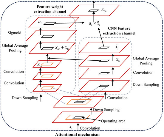
Figure 2.
Schematic diagram of attention-mechanism-based feature fusion block.
As depicted in Figure 2, the input feature learned from the front network is described as . After obtaining , a normal two-layer down-sampling block is firstly applied to update the learned feature. Then, two different processes are applied to the updated feature. In this processing step, a further down sampling layer is used to learn the global information and a convolutional layer is used to learn the informative feature . Then, an updated feature is obtained after with other convolutional layers. After that, and are transformed into the same dimension and added together. Following that, a sigmoid layer is added to normalize the output to [0, 1]. Then the feature weight is obtained, which is used to further highlight the informative characteristics and suppress the noise. Finally, the feature is multiplied by the weight to obtain the final selected feature , which is also used as the input for the next layer. For multi-scale feature fusion, the N feature with N scales are concatenated together, and the concatenated feature is used as the input of the following fully connected layer.
2.2.2. Residual Learning Block
Residual learning was firstly proposed by He et al. [26] to address the problems of gradient vanishing and explosion. The schematic diagram of its network module is given in Figure 3. As the figure shows, the input feature is set as and the output feature is set as , which is also the input of next layer. is the layer function without residual learning operation with two convolutional layers and one relu-nonlinear activation layer. The skip connection on the right side is called shortcut cross-layer connection, which is performed as an extra feature learning operation using a convolutional layer with kernel size. represents the shortcut cross-layer function. Finally, the output feature can be obtained as . With shortcut cross-layer connection, the block can be used to learn more information of the target and improve the recognition accuracy. In view of this, we add a residual learning module to each convolution layer to improve the feature learning ability.
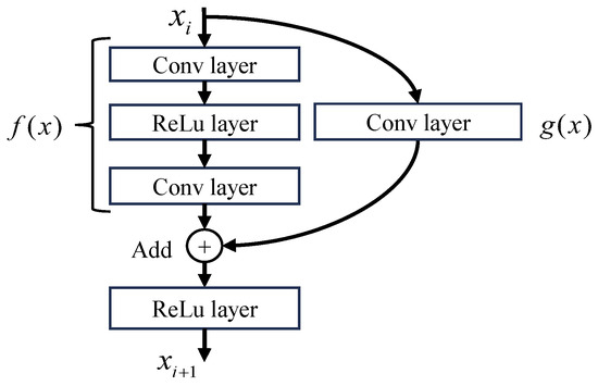
Figure 3.
Schematic diagram of residual learning block [26].
2.2.3. Function-Weighted Cross-Entropy Loss Function
As can be seen from Figure 1, the network model framework can be generally divided into front-end network and back-end loss function. To deal with the data imbalance, -function-weighted cross-entropy loss function is proposed here. Suppose the probability that a given sample belongs to class B is , the sample is easy to classify when , while it is difficult to classify when . The cross-entropy loss obtains a small loss value on the easily classified classes, and the model benefits little. However, in reality, there are often more easy categories and fewer hard categories. As a result, these small loss values would overwhelm the hard categories in the recognition part. However, the hard samples are often important samples for special tasks. Therefore, in the new loss function CFWCEL, the hard samples obtained much more attention by increasing their loss weight. In detail, the loss of the easily classified samples is smaller and declines faster, and the loss of the hard classified samples declines slowly to learn more category information. The CFWCEL is defined as:
where is the prediction probability of a given sample and . is the standard cross-entropy loss and is the added weighted factor to readjust the weight of cross entropy loss. In detail, is the regulator of , which takes odd and even numbers greater than 0. is the hyperparameter, which can be any value in general. In particular, when is 0, the CFWCEL turns out to be the standard cross-entropy loss. The optimal values of and are mutually influenced. The two parameters need to be adjusted in combination when evaluating the accuracy. It can be found that is a periodic function, whose period is adjusted by adjusting the values of and .
Figure 4 shows the CFWCEL results with different and . We can see that when and , the result of CFWCEL appears negative and its monotonicity changes. A similar result is obtained with and . When , due to the duality of even-order function, the negative results do not appear, but the monotonicity still changes. As a result, the value of should satisfy that . Among , CFWCEL decreases fastest when . Consequently, in our experiments is set to .
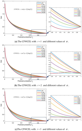
Figure 4.
The CFWCEL results with different and .
Figure 5 shows the CFWCEL results with different under . It can be seen that the CFWCEL decreases fast as increases. However, when and , CFWCEL decreases too fast and almost turns to 0. Such characteristic makes CFWCEL unable to distinguish target information in extremely unbalanced data, which is not conducive to the target recognition task. To avoid this situation, is set to 2. Finally, CFWCEL is set to in our paper.
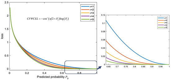
Figure 5.
The CFWCEL results with different and .
Figure 6 illustrates the comparison results between CFWCEL and other loss functions in terms of absolute and relative loss value. In the comparison, the loss functions are set as following:
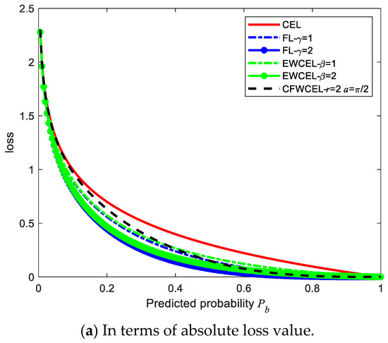
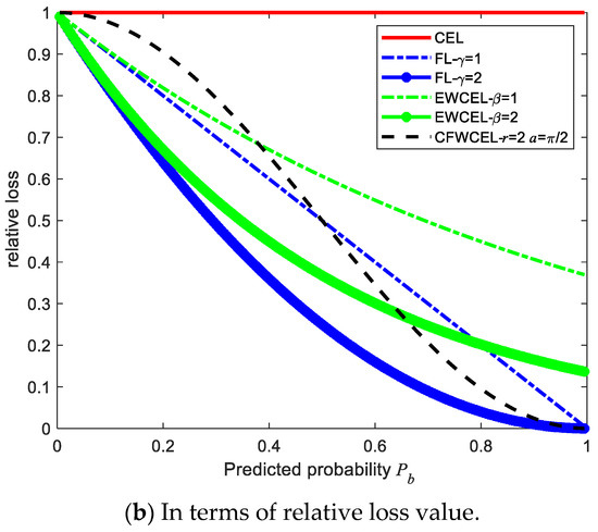
Figure 6.
The comparison results between CFWCEL and other loss functions.
Figure 6a shows the absolute value of each loss function, while Figure 6b displays the value of each loss function relative to CEL. We can see that CFWCEL obtains the largest absolute gradient at , which is exactly the boundary between the easy samples and the hard samples. It means that CFWCEL is more sensitive to the difference between easy samples and hard samples. Actually, CFWCEL pays more attention to the samples which are difficult to separate and can better adjust their weights. It can also be seen that this difference between easy samples and hard samples is obviously larger than EWCEL [10] and Focal Loss [12], so CFWCEL is more suitable for an imbalanced dataset.
2.2.4. The Whole Network
With the attention-mechanism-based multi-scale feature fusion and residual learning block, a multi-scale residual-convolutional neural network with embedded attention mechanism (MR-CNN-A) is proposed for underwater target recognition, as shown in Figure 7. MR-CNN-A is designed under a three-layer convolutional neural network (marked as Simple-CNN model) [9,27], which is a common model for underwater acoustic target recognition. In MR-CNN-A, the backbone feature extraction network consists of three convolution layers with three convolution kernels of different sizes (like 3 × 3, 5 × 5 and 7 × 7, respectively). These kernels ensure the extraction of multi-scale features. For each convolutional module, a residual learning block is added. After the backbone feature extraction network, the attention-mechanism-based feature fusion module is followed to fuse the obtained features. Then, a fully connected layer with a nonlinear activation function is added to the network. Finally, a fully connected layer with softmax is used as a classifier. ReLu nonlinear activation function layer is used in each convolutional operation except the last fully connected layer. ReLu plays an important role in decision-making and speeds up the learning process. It should be noted that the loss function adopted in the experiments in this paper is somewhat different and is explained in the following part. It is obvious that this model can theoretically realize noise resistance and achieve high robustness classification.
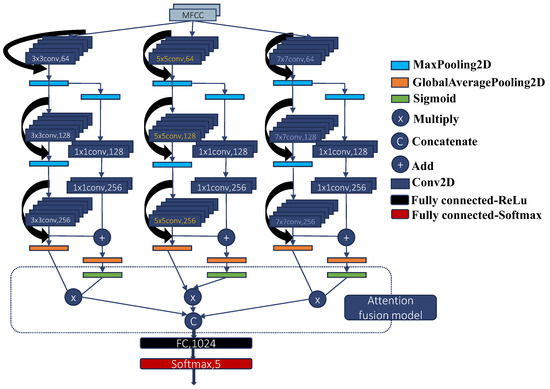
Figure 7.
The structural diagram of MR-CNN-A network.
3. Results and Discussions
In this paper, two underwater acoustic data sets are used to verify this method: ShipsEar [28] and Autonomous Underwater Vehicle (AUV) noise data.
ShipsEar [28]: It contains 11 kinds of ship audio data collected by a passive sonar in the underwater environment, including 90 audio messages, such as ocean liner, pilot ship and underwater background noise. Each message is divided into five categories according to its size: Tiny class A (fishing boats, trawlers, mussel boats, tugboats and dredgers), Average category B (motor boats, pilot boats and sailing vessels), Large category C (passenger ferry), Larger category D (Ocean Liners and Ro-Ro Ships), and class E (background noise).
AUV dataset: The Autonomous Underwater Vehicle (AUV) noise data are collected in a lake by our designed passive sonar. They are collected by a passive sonar-fiber hydrophone with a sampling frequency of 50 kHz. The AUV speed is set to 3 knots or 5 knots. The depth of AUV is set to 0, 5, 10 m, respectively. The data are labeled to two categories: Surface and underwater.
In the experiments, MR-CNN-A without CFWCEL is valued with a single feature first. Then, MR-CNN-A with CFWCEL is valued. The software platform for the experiments in this paper is TensorFlow. The hardware platform is a desktop computer with 16 G memory and GTX1080 graphics card. The support vector machine (SVM) multi-classification is trained using multi-class error-correcting output code (ECOC) model [29] through binary learners with standard linear classification. The evaluation standard is the target recognition accuracy.
3.1. Comparison of Feature Extraction Methods
The adaptation performance of MFCC, DEMON, and HHT features are analyzed firstly.
In this experiment, to exclude the influence of data imbalance, the 90 pieces of data in ShipsEar are simply split, and each category retains 266 samples with a total sample number of 1330. In AUV dataset, the same simple processing is performed as above, keeping the total number of samples at 1462 and the number of each category at 731. Moreover, 20% of the data is used for testing, and 80% of the data is used for training in the two datasets. The recognition class in ShipsEar is set to 5, while the recognition class in AUV is set to 2. The training learning rate is 0.001 and the number of epochs is set to 100. Moreover, the loss function is set as cross-entropy loss.
For ShipsEar dataset, the dimension of MFCC used here is (98, 12), where 98 represents the number of frames and 12 represents the dimension of MFCC feature eigenvalue. The dimension of DEMON used here is (60, 50) and the dimension of HHT is (16, 350). For AUV dataset, the dimension of MFCC, DEMON, and HHT is changed to (93, 12), (60, 50), and (14, 350), respectively. Table 1 shows the recognition experiment results.

Table 1.
Recognition results from different feature extraction methods.
As seen from Table 1, DEMON with SVM [29] obtains the best recognition results on the two datasets among the three features, 86.06% on the ShipsEar and 84.86% on the AUV dataset. At the same time, when the Simple-CNN model [9,27] is used as the classifier, MFCC with Simple-CNN model achieves the best recognition results, 96.24% on the ShipsEar and 92.12% on the AUV dataset. It means that DEMON is suitable for SVM, and MFCC is suitable for the CNN model. As a result, the MFCC is used as the input of our proposed network MR-CNN-A.
3.2. Comparison of Classification Methods
To verify the superiority of MR-CNN-A, the experiments with only MFCC feature are performed. For the network, MFCC is set as the only input of MR-CNN-A, and the loss function is set as cross-entropy loss. The setting of the dataset and feature extraction is the same as Section 3.1.
3.2.1. Experimental Results with Different Methods
The experimental results of different methods with MFCC on the two datasets are shown in Table 2.

Table 2.
Experimental results with MFCC.
On the ShipsEar dataset, both MR-CNN-A and Simple-CNN models [9,27] obtain a higher recognition rate (96.24%, 98.87% respectively) than the traditional SVM (81.58%) [29], with a greater improvement than 15%. These results verify the superiority of the deep learning method. Compared with Simple-CNN, MR-CNN-A also achieves an improvement of 2.63%. A similar result is obtained on the AUV dataset. On the AUV dataset, MR-CNN-A makes a 17.1% improvement over SVM and a 6.14% improvement over Simple-CNN. It demonstrates that MR-CNN-A gains much more robust features.
Using the results on ShipsEar as a baseline for comparison, the recognition accuracy of Simple-CNN on AUV dataset decreases by 4.12%, while the recognition performance of MR-CNN-A on AUV dataset only decreases by 0.61%. That means the feature extracted by MR-CNN-A is more discriminating and stable than the feature extracted by the Simple-CNN model. It is indirectly verified that the designed attentional-mechanism-based fusion module acts as a feature selector to suppress noise. The fusion module rebalances the feature weight, thus improving the recognition performance. The addition of residual learning also proves that it can greatly reduce the training error and enhance recognition accuracy.
3.2.2. Experimental Results with Different Noise Levels
In order to further verify the robustness of MR-CNN-A, the above recognition experiments were re-conducted with different gaussian noise levels on the ShipsEar dataset. The noise level is described using the Signal to Noise Ratio (SNR). In the experiments, white gaussian noise with specified power is added to the original audio data.
The experimental results under different SNR are given in Table 3. It can be seen that MR-CNN-A is significantly superior to the Simple-CNN model [9,27] and SVM [29] in the case of low SNR level. Among all the noise level, MR-CNN-A all achieves the best result. Especially when SNR is −10 dB, MR-CNN-A also achieves the best result with an accuracy of 88.36%. When SNR = −1 dB, −2 dB, −3 dB, compared with Simple-CNN, MR-CNN-A achieves an improvement of more than 10%. Moreover, as the noise level increases, the recognition results obtained by MR-CNN-A decline more slowly than Simple-CNN and SVM. This also verifies that the attention-based-fusion block has a high tolerance to noise, which can extract features with high robustness under the condition of low SNR.

Table 3.
Experimental results on ShipsEar under different SNR.
3.3. Experiments with Different Imbalanced Data
3.3.1. Data Imbalance Definition
Before the experiments, we first give the definition of data imbalance. As shown in Equation (2), the data imbalance is measured as the degree of imbalance using the standard deviation of given samples, where represents the total number of categories and represents the sample proportion of class in whole samples. represents the average proportion of all categories, then measured the distance from the mean value.
From Equation (2), we can see that satisfies the following three properties:
(1) In general, .
(2) When the data are balanced with , .
(3) The value of has nothing to do with the order of . That means, when the proportions of different types are exchanged with each other, remains unchanged, .
For example, assuming that there are five types of targets, accounting for 10%, 20%, 30%, 30% and 10% of the total 3000 samples, respectively, then . In particular, considering (0, 0, 0, 100%, 0), . Therefore, for the five categories, the highest value of disequilibrium degree is 0.8944.
3.3.2. Parameter Selection in CFWCEL
In this part, we verify the influence of parameter of CFWCEL in the imbalanced data experiments. With the same degree of and different value of , the recognition performance of MR-CNN-A is tested, and Figure 8 presents the results. The dataset is extracted from ShipsEar with a setting of and the total number of samples is 1500 with 80% for training and 20% for testing. The other setting of the network is the same as the setting in Section 3.1. Two cases are used to verify the performance of CFWCEL, that are and . Meanwhile, is set to .
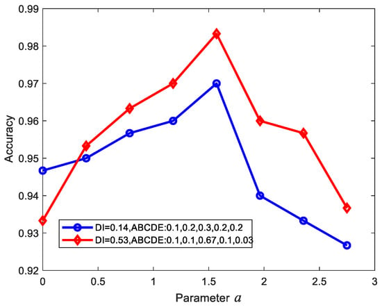
Figure 8.
Recognition results with different CFWCEL parameter under different .
It can be seen from Figure 8 that when (which means CFWCEL turns to be cross entropy loss), the greater the is, the lower recognition performance is obtained. When is , the best recognition result is obtained in each situation. As a result, is set to in our imbalanced data experiments.
3.3.3. Imbalanced Data Experiments
In this part, the performance of CFWCEL is tested under different and a comparison with other loss function is also applied. The network and the dataset parameters are the same as the parameters in Section 3.3.2. There are 1500 samples with five classes (A, B, C, D, E) in the dataset and 1000 samples for training while 500 samples for tests. The is changed by changing the distribution of each class sample in the training data part, while the in test data part is set to 0. The details of 10 types of setting are displayed in Table 4.

Table 4.
The data distribution of each used dataset and its DI.
Figure 9 shows the recognition accuracy of four loss functions, like cross-entropy loss, CFWCEL (), Focal Loss () [12] and EWCEL () [10]. From Figure 9, it can be observed that no matter what kind of loss function is used, the recognition performance always decreases when DI increases. The realization of the anti-imbalance loss function can only suppress the occurrence of this decrease and improve the recognition rate relatively. It can also be seen that when , the results of CFWCEL, EWCEL, and Focal Loss are almost the same, and all of them are higher than 90%. When , CFWCEL shows a clear superiority among the four loss functions. In detail, the recognition accuracy of CFWCEL is higher than the other functions by about 1–3.5%. These results effectively verify the effectiveness of CFWCEL. When DI increases, CFWCEL prompts MR-CNN-A to pay more attention to hard samples.
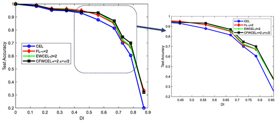
Figure 9.
The recognition performance of four loss functions under different .
4. Conclusions
To address the low feature expressiveness and poor robustness caused by data imbalance, a multi-scale feature fusion residual convolutional neural network (MR-CNN-A) and a trigonometric weighted cross-entropy loss function (CFWCEL) are proposed. Firstly, MFCC is used to suppress the low-frequency feature of underwater acoustic objects. Secondly, the attention module is used to rebalance the weight of each feature dimension to achieve robust multi-scale feature extraction. Then, CFWCEL is used to realize imbalanced data feature learning. MR-CNN-A takes sufficient advantage of the input feature (MFCC) through multi-scale attention-operations-based feature fusion, and searches for useful features of imbalanced data adaptively through the use of CFWCEL. Experimental results and analyses on the open source ShipsEar dataset and self-collected AUV dataset show that MR-CNN-A achieves the best results among other methods, like SVM [29] and Simple-CNN model [9,27]. It is worth noting that MR-CNN-A shows good stability against gaussian noise and data imbalance. In future research, MR-CNN-A and CFWCEL will be generalized and verified on other different datasets.
Author Contributions
Y.Z. and M.L. contributed equally to this work. Conceptualization, Y.M., M.L. and Y.Z.; methodology, Y.M., M.L. and Y.Z.; software, Y.M., M.L. and Y.Z.; validation, Y.M., M.L., Y.Z., B.Z. (Bingbing Zhang), K.X., B.Z. (Bo Zou) and Z.H.; formal analysis, K.X., B.Z. (Bo Zou) and Z.H.; investigation, K.X., B.Z. (Bo Zou) and Z.H.; resources, K.X., B.Z. (Bo Zou) and Z.H.; data curation, Y.M., M.L. and Y.Z.; writing—original draft preparation, Y.M., M.L. and Y.Z.; writing—review and editing, Y.M., M.L. and Y.Z.; visualization, Y.M., M.L. and Y.Z.; supervision, K.X., B.Z. and Z.H.; project administration, Y.M., K.X., B.Z. (Bo Zou) and Z.H.; funding acquisition, Y.M., B.Z. (Bingbing Zhang), K.X. and Z.H. All authors have read and agreed to the published version of the manuscript.
Funding
This research was funded by the Research Program of NUDT No. ZK20-39, No. ZK20-35, No. ZK19-36, the National Natural Science Foundation of China under grant number 61905283 and the Changsha Municipal Natural Science Foundation No. kq2202067.
Data Availability Statement
Not applicable.
Conflicts of Interest
The authors declare no conflict of interest.
References
- Luo, X.; Zhang, M.; Liu, T.; Huang, M.; Xu, X. An Underwater Acoustic Target Recognition Method Based on Spectrograms with Different Resolutions. J. Mar. Sci. Eng. 2021, 9, 1246. [Google Scholar] [CrossRef]
- Zhang, W.; Wu, Y.; Shi, J.; Leng, H.; Zhao, Y.; Guo, J. Surface and Underwater Acoustic Source Discrimination Based on Machine Learning Using a Single Hydrophone. J. Mar. Sci. Eng. 2022, 10, 321. [Google Scholar] [CrossRef]
- Su, T. Multiple neural networks-integrated underwater target classification based on fuzzy theory. J. Acoust. Soc. Am. 2000, 107, 2868. [Google Scholar] [CrossRef]
- Bianco, M.J.; Gerstoft, P.; Traer, J.; Ozanich, E.; Roch, M.A.; Gannot, S.; Deledalle, C.-A. Machine learning in acoustics: Theory and applications. J. Acoust. Soc. Am. 2019, 146, 3590–3628. [Google Scholar] [CrossRef] [PubMed] [Green Version]
- Wu, Y.; Li, X.; Wang, Y. Extraction and classification of acoustic scattering from underwater target based on Wigner-Ville distribution. Appl. Acoust. 2018, 138, 52–59. [Google Scholar] [CrossRef]
- Li, S.; Yang, S.; Liang, J. Recognition of ships based on vector sensor and bidirectional long short-term memory networks. Appl. Acoust. 2020, 164, 107248. [Google Scholar] [CrossRef]
- Ferguson, E.L.; Ramakrishnan, R.; Williams, S.B.; Jin, C.T. Deep learning approach to passive monitoring of the underwater acoustic environment. J. Acoust. Soc. Am. 2016, 140, 3351. [Google Scholar] [CrossRef]
- Yang, K.; Zhou, X. Deep learning classification for improved bicoherence feature based on cyclic modulation and cross-correlation. J. Acoust. Soc. Am. 2019, 146, 2201–2211. [Google Scholar] [CrossRef]
- Wu, H.; Song, Q.; Jin, G. Deep Learning based Framework for Underwater Acoustic Signal Recognition and Classification. In Proceedings of the 2018 2nd International Conference on Computer Science and Artificial Intelligence, Hohhot, China, 22–24 October 2018; pp. 385–388. [Google Scholar] [CrossRef]
- Dong, Y.; Shen, X.; Jiang, Z.; Wang, H. Recognition of imbalanced underwater acoustic datasets with exponentially weighted cross-entropy loss. Appl. Acoust. 2020, 174, 107740. [Google Scholar] [CrossRef]
- Oksuz, K.; Cam, B.C.; Kalkan, S.; Akbas, E. Imbalance Problems in Object Detection: A Review. IEEE Trans. Pattern Anal. Mach. Intell. 2021, 43, 3388–3415. [Google Scholar] [CrossRef] [Green Version]
- Lin, T.Y.; Goyal, P.; Girshick, R.; He, K.; Dollar, P. Focal loss for dense object detection. IEEE Trans. Pattern Anal. Mach. Intell. 2020, 42, 318–327. [Google Scholar] [CrossRef] [PubMed] [Green Version]
- Barandela, R.; Rangel, E.; Sánchez, J.S.; Ferri, F.J. Restricted Decontamination for the Imbalanced Training Sample Problem. In Progress in Pattern Recognition, Speech and Image Analysis (CIARP); Springer: Berlin/Heidelberg, Germany, 2003; Volume 2905, pp. 424–431. [Google Scholar] [CrossRef] [Green Version]
- Buda, M.; Maki, A.; Mazurowski, M.A. A systematic study of the class imbalance problem in convolutional neural networks. Neural Networks 2018, 106, 249–259. [Google Scholar] [CrossRef] [PubMed] [Green Version]
- Huang, C.; Li, Y.; Loy, C.C.; Tang, X. Learning Deep Representation for Imbalanced Classification. In Proceedings of the 2016 IEEE Conference on Computer Vision and Pattern Recognition (CVPR), Las Vegas, NV, USA, 26 June–1 July 2016; pp. 5375–5384. [Google Scholar]
- Huang, C.; Li, Y.; Loy, C.C.; Tang, X. Deep Imbalanced Learning for Face Recognition and Attribute Prediction. IEEE Trans. Pattern Anal. Mach. Intell. 2019, 42, 2781–2794. [Google Scholar] [CrossRef] [PubMed] [Green Version]
- Li, B.; Liu, Y.; Wang, X. Gradient Harmonized Single-Stage Detector. In Proceedings of the Thirty-Third AAAI Conference on Artificial Intelligence (AAAI2019), Hilton Hawaiian Village, Honolulu, HI, USA, 27 January–1 February 2019; Volume 33, pp. 8577–8584. [Google Scholar]
- Jensen, J.; Tan, Z.-H. Minimum Mean-Square Error Estimation of Mel-Frequency Cepstral Features–A Theoretically Consistent Approach. IEEE/ACM Trans. Audio Speech Lang. Process. 2015, 23, 186–197. [Google Scholar] [CrossRef]
- Brown, G.J.; Mill, R.W.; Tucker, S. Auditory-motivated techniques for detection and classification of passive sonar signals. J. Acoust. Soc. Am. 2008, 123, 3344. [Google Scholar] [CrossRef] [Green Version]
- Zhang, L.; Wu, D.; Han, X.; Zhu, Z. Feature Extraction of Underwater Target Signal Using Mel Frequency Cepstrum Coefficients Based on Acoustic Vector Sensor. J. Sensors 2016, 2016, 7864213. [Google Scholar] [CrossRef] [Green Version]
- Yan, J.; Sun, H.; Cheng, E.; Kuai, X.; Zhang, X. Ship Radiated Noise Recognition Using Resonance-Based Sparse Signal Decomposition. Shock Vib. 2017, 2017, 6930605. [Google Scholar] [CrossRef] [Green Version]
- Wang, W.; Zhao, X.; Liu, D. Design and Optimization of 1D-CNN for Spectrum Recognition of Underwater Targets. Integr. Ferroelectr. 2021, 218, 164–179. [Google Scholar] [CrossRef]
- Vaswani, A.; Shazeer, N.; Parmar, N.; Uszkoreit, J.; Jones, L.; Gomez, A.N.; Kaiser, L.; Polosukhin, I. Attention is All You Need. In Proceedings of the Neural Information Processing Systems, Long Beach, CA, USA, 4–9 December 2017; pp. 5998–6008. [Google Scholar]
- Jaderberg, M.; Simonyan, K.; Zisserman, A.; Kavukcuoglu, K. Spatial Transformer Networks. In Proceedings of the Neural Information Processing Systems, Montreal, QC, Canada, 7–12 December 2015; pp. 2017–2025. [Google Scholar]
- Hu, J.; Shen, L.; Albanie, S.; Sun, G.; Wu, E. Squeeze-and-Excitation Networks. IEEE Trans. Pattern Anal. Mach. Intell. 2017, 42, 2011–2023. [Google Scholar] [CrossRef] [Green Version]
- He, K.; Zhang, X.; Ren, S.; Sun, J. Deep residual learning for image recognition. In Proceedings of the 2016 IEEE Conference on Computer Vision and Pattern Recognition (CVPR), Las Vegas, NV, USA, 26 June–1 July 2016; pp. 770–778. [Google Scholar] [CrossRef] [Green Version]
- Jiang, J.; Shi, T.; Huang, M.; Xiao, Z. Multi-scale spectral feature extraction for underwater acoustic target recognition. Measurement 2020, 166, 108227. [Google Scholar] [CrossRef]
- Santos-Domínguez, D.; Torres-Guijarro, S.; Cardenal-López, A.; Pena, A. ShipsEar: An underwater vessel noise database. Appl. Acoust. 2016, 113, 64–69. [Google Scholar] [CrossRef]
- Escalera, S.; Pujol, O.; Radeva, P. Separability of ternary codes for sparse designs of error-correcting output codes. Pattern Recognit. Lett. 2009, 30, 285–297. [Google Scholar] [CrossRef]
Publisher’s Note: MDPI stays neutral with regard to jurisdictional claims in published maps and institutional affiliations. |
© 2022 by the authors. Licensee MDPI, Basel, Switzerland. This article is an open access article distributed under the terms and conditions of the Creative Commons Attribution (CC BY) license (https://creativecommons.org/licenses/by/4.0/).