Spectral-Spatial Interaction Network for Multispectral Image and Panchromatic Image Fusion

Abstract

Recently, with the rapid development of deep learning (DL), an increasing number of DL-based methods are applied in pansharpening. Benefiting from the powerful feature extraction capability of deep learning, DL-based methods have achieved state-of-the-art performance in pansharpening. However, most DL-based methods simply fuse multi-spectral (MS) images and panchromatic (PAN) images by concatenating, which can not make full use of the spectral information and spatial information of MS and PAN images, respectively. To address this issue, we propose a spectral-spatial interaction Network (SSIN) for pansharpening. Different from previous works, we extract the features of PAN and MS, respectively, and then interact them repetitively to incorporate spectral and spatial information progressively. In order to enhance the spectral-spatial information fusion, we further propose spectral-spatial attention (SSA) module to yield a more effective spatial-spectral information transfer in the network. Extensive experiments on QuickBird, WorldView-4, and WorldView-2 images demonstrate that our SSIN significantly outperforms other methods in terms of both objective assessment and visual quality.

1. Introduction

Due to the limitations of remote sensing satellite-imaging system, remote sensing satellite images with both high spatial and high spectral resolution are difficult to obtain. This problem can be mitigated by improving the hardware. However, it turns out to be an arduous task due to the strict limit of the signal-to-noise ratio of satellite products [1]. To alleviate this problem, the pansharpening technique was proposed. The main purpose of pansharpening is to generate a high-spatial-resolution (HR) multispectral (MS) image, which contains spatial information of the panchromatic (PAN) image and spectral information of the corresponding MS images, by fusing a low-spatial-resolution (LR) MS image with a HR PAN image. As one of the most basic and dynamic research topics in remote sensing, pansharpening has a significant impact on many remote sensing applications, such as crop mapping [2], land cover classification [3], and target detection [4]. In recent years, with the wide application of deep learning in various computer vision tasks, DL-based pansharpening methods have developed rapidly. Inspired by SRCNN [5], Masi et al. [6] first attempted to use convolutional neural networks (CNN) for pansharpening and stacks of three convolutional layers (PNN) for pansharpening, achieving state-of-the-art results. Motivated by the results of the PNN, many pansharpening methods based on deep learning have emerged in recent years [7,8,9,10,11,12,13].

Although they have different structures and achieve the desired effect, they usually underutilize the advantage of spectral information that exists in the MS images and spatial information that exists in the PAN images. Most of them tend to concatenate PAN and MS images at the beginning of the network and extract the input feature maps with a single network, which is simple and easy to implement but is not conducive to spectral-spatial information fusion. Even though some DL-based methods [14,15,16,17,18] are designed to be multi-branch structures, and the features of the input PAN and MS images are extracted respectively, they fail to consider the interaction and the impact of spectral-spatial information, which is adverse to information transmission and conversion in networks.

In view of the above issues, we propose a spectral-spatial interaction network for pansharpening. Specifically, to fully extract the features of MS and PAN images, SSIN is designed as dual-branch structures, where the spatial branch is used to extract spatial information from PAN images and the spectral branch extracts spectral information from MS images. Inspired by [19], we take into account information guidance between different branches and design a spectral-spatial attention (SSA) module to fully extract the advantageous information from the two branches. Moreover, we introduce an information interaction block (IIB) into our network for information interaction of the spectral branch and spatial branch. Furthermore, we assemble IIB and SSA into an information interaction group (IIG) as the basic structure of our network. It is worth noting that we use a long skip connection to pass the upsampled MS image to the end of the network directly; many DL-based methods [8,20,21,22] have demonstrated the effectiveness of this approach.

In summary, the main contributions of this article are as follows:

(1)

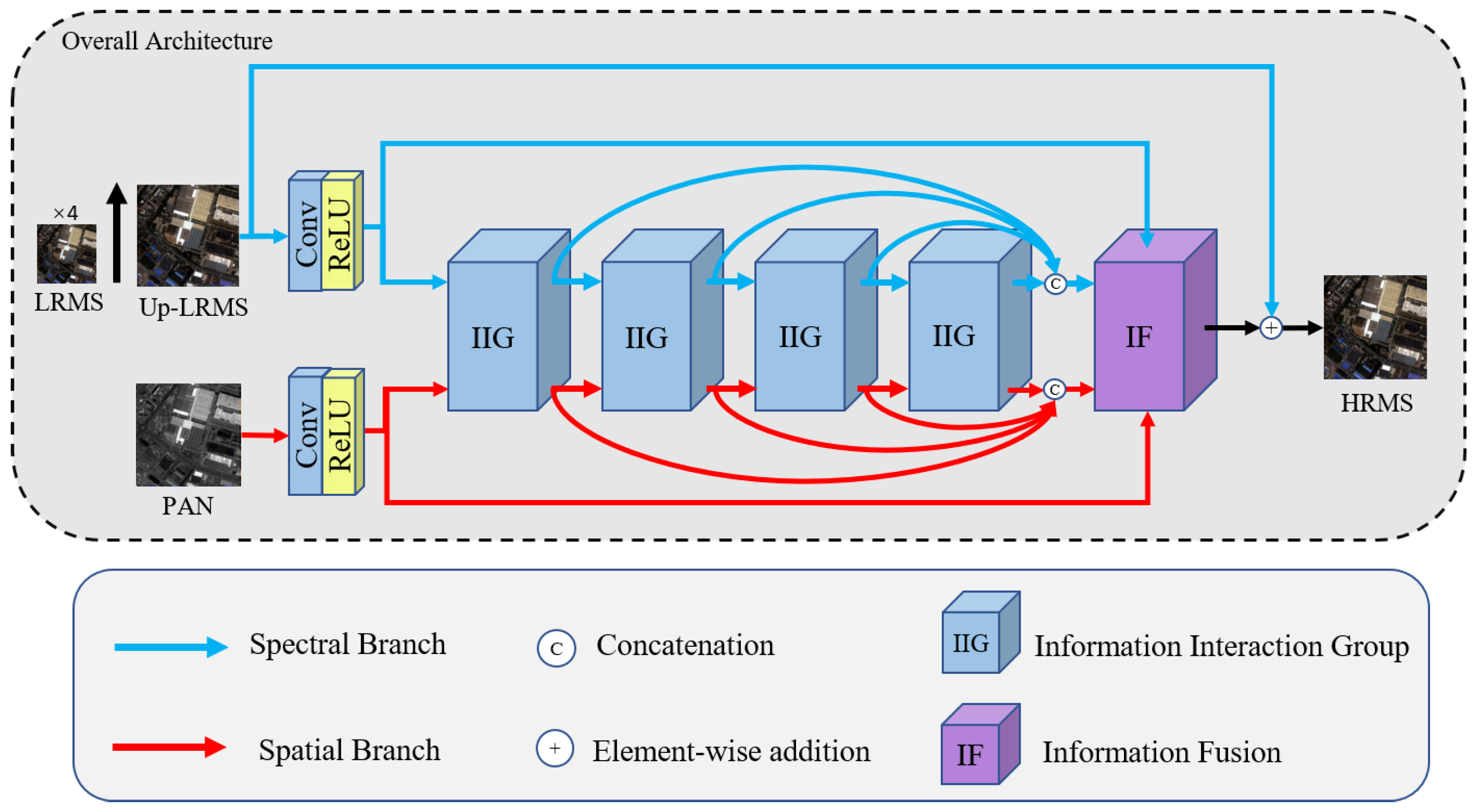
We propose a spectral-spatial interaction network (SSIN) based on information interaction group for pansharpening. The network is designed as a dual-branch architecture. It extracts spectral and spatial information independently from the two branches and are interacted repetitively to incorporate spectral and spatial information progressively.

(2)

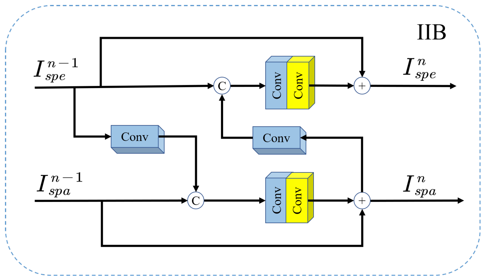
We propose the information interaction block (IIB) to enhance the conversion and transmission of spectral and spatial information between the two branches. Because it is a dual-input and dual-output structure, it can be embedded in dual-branch networks efficiently.

(3)

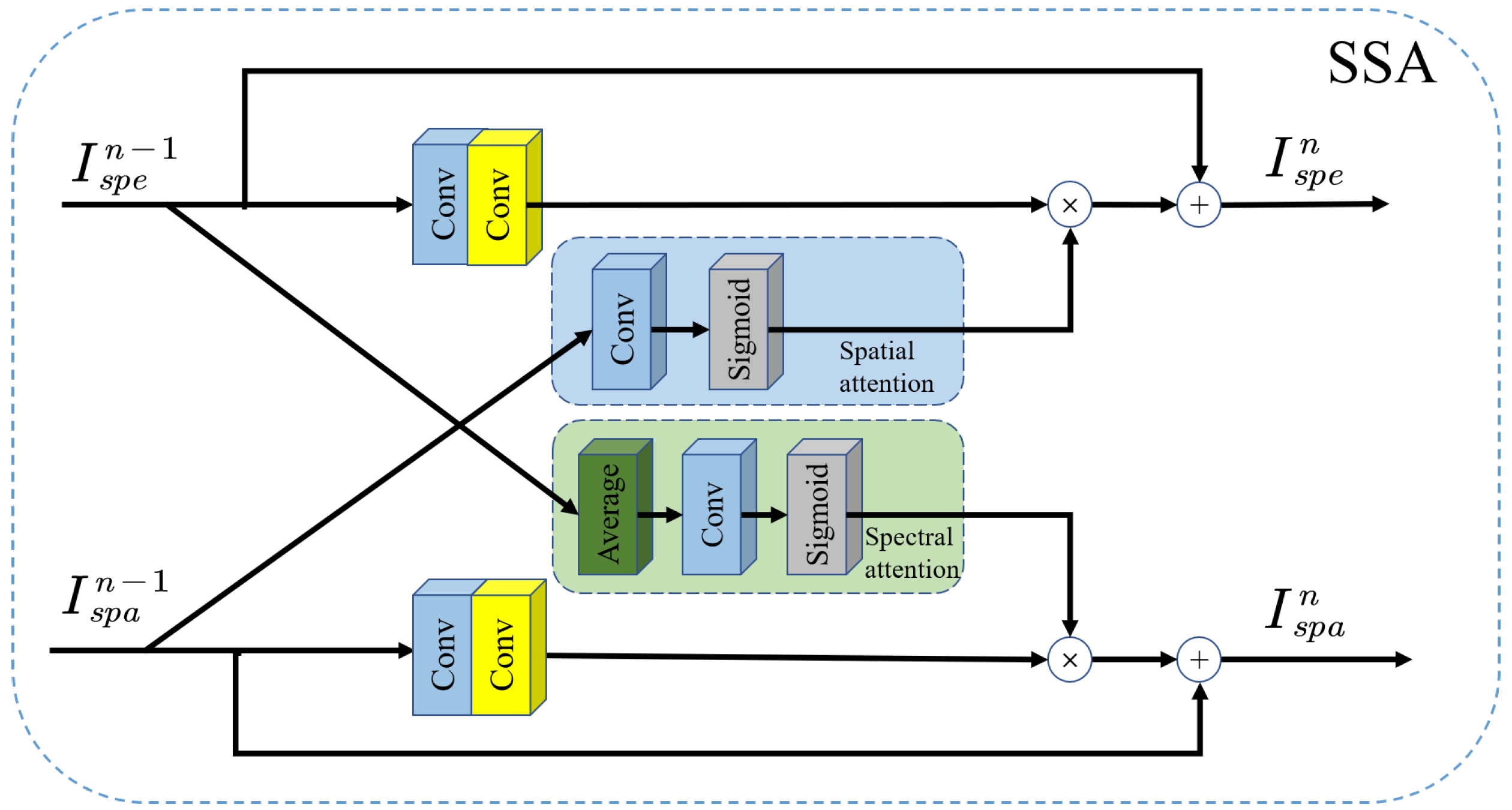
We design a lightweight and effective spectral-spatial attention module, which is able to calculate spatial attention from the PAN branch to guide the MS branch. Similarly, it calculates spectral attention from the MS branch to guide the PAN branch. In this way, the advantages of information of MS and PAN images can be fully utilized, which facilitates the fusion of different information.

The remainder of this paper is organized as follows. Section 2 introduces the related work, while Section 3 introduces the proposed SSIN and each part of the network in detail. Section 4 presents the data sets, evaluation index, ablation study, parameters analysis and comparison with SOTA methods on three data sets. Section 5 presents the efficiency study. Finally, Section 6 draws conclusions.

2. Related Work

Over the past decades, many pansharpening methods have been put forward. These methods fall into four categories [23]: component substitution (CS)-based methods, multi-resolution analysis (MRA)-based methods, variational optimization (VO)-based methods, and deep learning (DL)-based methods. In CS-based methods, the LR MS image is decomposed into spectral and spatial components, then the decomposed spatial components of the LR MS image are replaced by the histogram-matched PAN image. Finally, the HR MS image is obtained by inverse transformation. Several widely known CS-based methods include intensity-hue-saturation (IHS) [24,25], principal component analysis (PCA) [26], the Gram–Schmidt (GS) conversion [27], the adaptive GS (GSA) [28], the partial replacement adaptive CS (PRACS) [29], and the band-dependent spatial details (BDSD) [30]. These CS-based methods are simple and efficient and can directly extract spatial information from PAN images. However, spectral distortion is prone to occurs during pansharpening when the correlation between the PAN and MS images is low [31]. As for MRA-based methods, MRA-based methods typically consist of three steps: (1) the upsampled MS image and PAN image are decomposed into multiple scales, (2) fusion at every scale, (3) utilizes an inverse transform to get the reconstructed image. MRA-based methods use multi-scale decomposition to decompose the source image into multiple scales, for instance, discrete wavelet transform (DWT) [32], Laplacian pyramid (LP) [33], generalized Laplacian pyramid (GLP) [34], and contourlet transformation [35]. These methods are generally superior to CS-based methods in spectral fidelity. However, multiscale transformation brings a large amount of computation and may lead to spatial distortion [36].

In order to balance spectral and spatial distortions, some methods based on variational optimization are proposed.

VO-based pansharpening methods transformed the pansharpening process into an optimization problem. The key to solve the problem is the establishment of energy function and the selection of optimization algorithm [37].

This category was developed in the 1990s [38]. Since Ballester et al. [39] proposed the pioneer variational method for pansharpening, VO-based pansharpening methods attracted more and more attention and developed rapidly. Model-based methods [40,41] and sparse-based methods [42,43] are two representative VO-based methods. Even though VO-based methods can produce high-quality fusion results, the optimization is time-consuming [44].

In recent years, with the rapid development of DL-based image super-resolution, many DL-based pansharpening methods have been put forward which greatly improve the performance and efficiency of pansharpening. Masi et al. [6] first introduced a simple three-layer CNN into pansharpening. Inspired by VDSR [20], Wei et al. [8] proposed a deep residual neural network with 11 convolutional layers for pansharpening. Yang et al. [7] proposed a deep network architecture for the pansharpening called PanNet, which trained the network in the high-pass domain to preserve the spatial structure. To capture multiscale detailed information, Yuan et al. [12] introduce multiscale feature extraction and residual learning into CNN for pansharpening. These pansharpening methods process at the pixel level. Different from the previous method, Liu et al. [13] presented a two-stream fusion network (TFNet) to fuse PAN and MS images in the feature level and reconstructed the pan-sharpened image from the fused features. To take full advantage of gradient characteristics in pansharpening. Lai et al. [45] utilized gradient information to guide the pansharpening process. The above method simply concatenated the upsampled MS image and PAN image, input it into the network, and then learned the mapping relationship between the input and HRMS image directly, which resulted in spatial distortion. To solve this problem. Wang et al. [15] integrated a multiscale U-shaped CNN into pansharpening for make full use of multispectral information. To explore the intra-image characteristics and the inter-image correlation concurrently. Guan et al. [46] proposed a three-stream structure network to fully extract the valuable information that encoded in the HR PAN images and LR hyperspectral images.

As mentioned above, although most of the current DL-based methods have significantly improved the fusion performance, they do not explore the advantage information of MS and PAN images. Unlike the above methods, we consider the interaction and impact of spectral-spatial information on the basis of the dual-branch structure. We use both spatial attention and spectral attention mechanisms in the SSA module to take full advantage of the advantageous information of the MS and PAN images.

3. Proposed Method

In this section, the implementation details of the SSIN will be described in detail, including the overall architecture, information interaction block (IIB), spectral-spatial attention (SSA) module, and information fusion (IF) module. We first introduce the overall structure of the network, and then the other network components in turn.

3.1. Network Architecture

Figure 1 shows the network architecture of SSIN, which consists of three main parts: spectral-spatial information extraction, spectral-spatial information interaction, and spatial-spectral information fusion. Specifically, we use a single convolutional layer to extract information and then stack the information interaction group (IIG) to achieve the information interaction. Finally, we use the IF module to fuse spectral and spatial information. The input LRMS image and PAN image are denoted as $I_{MS}\in {\mathbb{R}}^{h\times w\times c}$ and $I_{PAN}\in {\mathbb{R}}^{H\times W\times 1}$. The spectral and spatial information is first extracted by a single convolution layer, respectively.

$$I_{spe}^0=f_{spe}\left(f_{up}\left(I_{MS}\right)\right),I_{spa}^0=f_{spa}\left(I_{PAN}\right),$$

(1)

where $I_{spe}^0\in {\mathbb{R}}^{H\times W\times B}$ and $I_{spa}^0\in {\mathbb{R}}^{H\times W\times B}$ represent the extracted spectral and spatial information, respectively. $f_{spe}(·)$ and $f_{spa}(·)$ are $3\times 3$ convolutional layers used to extract the spectral-spatial information from the input image $I_{MS}$ and $I_{PAN}$. $f_{up}\left(·\right)$ represents the bicubic interpolation.

Then, the extracted spectral and spatial information are fed into a series of IIG to realize spectral-spatial information interaction, which can be formulated as follows:

$$\left(I_{spe}^n,I_{spa}^n\right)=f_{IIG}^n\left(I_{spe}^{n-1},I_{spa}^{n-1}\right),n=\left(1,2,...,N\right)$$

(2)

where $f_{IIG}^n\left(·\right)$ stands for the the $n^{th}$ IIG, and $I_{spe}^n$, $I_{spa}^n$ represent the output spectral and spatial information of the $n^{th}$ IIG, respectively. N denotes the total numbers of IIG.

Inspired by [47], we cascade all these IIGs to fully use the information interacted at different stages. Then, the spectral and spatial information extracted by each IIG are concatenated and fed into an information fusion module to fuse the spectral-spatial information. Simultaneously, we feed the spectral information $I_{spe}^0$ and spatial information $I_{spa}^0$ into the IF module to maintain the original information concentration. Finally, to maintain the integrity of the spectral information, we add the upsampled LRMS image to the fused information forming global residual learning. This process can be expressed as:

$$I_{fuse}=f_{IF}\left(\left[I_{spe}^1,\cdots ,I_{spe}^N\right],\left[I_{spa}^1,\cdots ,I_{spa}^N\right],I_{spe}^0,I_{spa}^0\right)$$

(3)

$$I_{SRMS}=I_{fuse}+f_{up}\left(I_{MS}\right)$$

(4)

where $f_{IF}\left(·\right)$ and $\left[·\right]$ denote the IF module and concatenation operation. $I_{fuse}$ represents the fused information by the IF module. $I_{SRMS}$ indicates the pansharpened MS image.

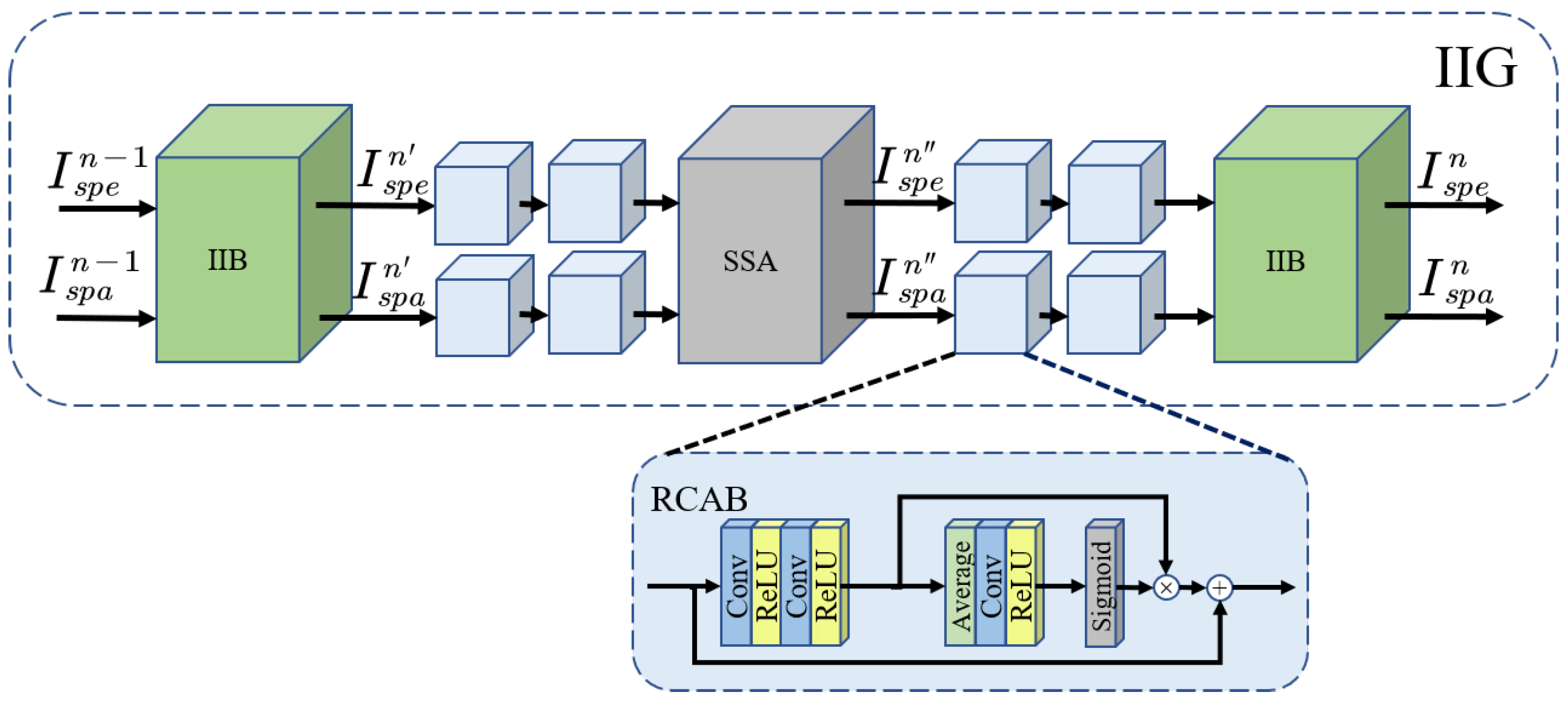
3.2. Information Interaction Group

Figure 2 shows the network architecture of the IIG, which is constructed by IIB, SSA, and residual channel attention blocks (RCABs) [48]. In IIG, the SSA is in the middle of two IIBs and connected by two cascade RCABs in each branch, which can be formulated as follows:

$$\left(I_{spe}^{n^{\prime }},I_{spa}^{n^{\prime }}\right)=f_{IIB,1}^n\left(I_{spe}^{n-1},I_{spa}^{n-1}\right)$$

(5)

$$\left(I_{spe}^{n^{″}},I_{spa}^{n^{″}}\right)=f_{SSA}^n\left(f_{RCAB}\left(I_{spe}^{{}^{\prime }}\right),f_{RCAB}\left(I_{spa}^{{}^{\prime }}\right)\right)$$

(6)

$$\left(I_{spe}^n,I_{spa}^n\right)=f_{IIB,2}^n\left(f_{RCAB}\left(I_{spe}^{n^{″}}\right),f_{RCAB}\left(I_{spa}^{n^{″}}\right)\right)$$

(7)

where $f_{IIB,1}^n(·)$, $f_{IIB,2}^n(·)$ represent the first and second IIB in IIG, respectively. $I_{spe}^{n^{\prime }}\left(I_{spa}^{n^{\prime }}\right)$ and $I_{spe}^{n^{″}}\left(I_{spa}^{n^{″}}\right)$ represent the intermediate process of IIG. $f_{RCAB}$ indicates two cascaded RCAB. The symmetrical structure of IIG is helpful to maintain the synchronization of spectral and spatial information.

3.3. Information Interaction Block

The main function of the IIB is to realize information interaction in SSIN. As shown in Figure 3, we first extract spectral information of the input spectral-branch feature by a convolutional layer with $3\times 3$ kernel size, then the extracted spectral information is concatenated with the input spatial-branch feature and further use a $1\times 1$ convolutional layer to update the spatial information. Note that we add the input spatial-branch feature to the updated spatial information to achieve local residual learning.

Simultaneously, we extract the spatial information of the spatial branch using a convolutional layer and then concatenated it with the input of the spectral-branch feature, but the difference is that we extract the spatial information of the spatial-branch output port. In this way, the updated spatial information can be used to guide spectral information updata. In summary, the information interaction block can be formulated as:

$$I_{spa}^n=\mathrm{Re}Lu\left(H_{1\times 1}\left(\left[H_{3\times 3}\left(I_{spe}^{n-1}\right),I_{spa}^{n-1}\right]\right)\right)+I_{spa}^{n-1}$$

(8)

$$I_{spe}^n=\mathrm{Re}Lu\left(H_{1\times 1}\left(\left[H_{3\times 3}\left(I_{spa}^n\right),I_{spe}^{n-1}\right]\right)\right)+I_{spe}^{n-1}$$

(9)

where $H_{1\times 1}$ and $H_{3\times 3}$ represent convolution operation with $1\times 1$ kernel size and $3\times 3$ kernel size, respectively. $\mathrm{Re}LU\left(·\right)$ represents the ReLU activation function [49].

3.4. Spectral-Spatial Attention Module

In order to take full advantage of the advantageous information of the spectral branch and spatial branch, we design a lightweight and effective spectral-spatial attention (SSA) module to guide spectral-spatial information integration. We compute the spatial and spectral attention from the branch of spatial and spectral, respectively. Then, we multiply the original features with the attention maps from another branch to transfer the corresponding information. Finally, we add the original features with the above weighted features in each branch to maintain the original information concentration. The schematic of SSA is shown in Figure 4.

Similar to [50], we use global average pooling and 1D convolution to achieve spectral attention which is lightweight and effective. The weights of spectral attention $w_{spe}\in {\mathbb{R}}^{1\times 1\times B}$ can be computed as:

$$w_{spe}=\delta \left(H_{1D}\left(g\left(I_{spe}^{n-1}\right)\right)\right)$$

(10)

where $g\left(x\right)=\frac{1}{WH}{\sum }_{i=1}^W{\sum }_{j=1}^H{I}_{spe\left(i,j\right)}^{n-1}$ is channel-wise global average pooling (GAP) and $\sigma$ is the Sigmoid function. $H_{1D}\left(·\right)$ indicates 1D convolution.

For spatial attention, we use $1\times 1$ convolution instead of the max pooling to generate the spatial attention map $w_{spa}\in {\mathbb{R}}^{H\times W\times 1}$. It can be formulated as:

$$w_{spa}=\delta \left(H_{1\times 1}\left(I_{spa}^{n-1}\right)\right)$$

(11)

To sum up, the spectral-spatial attention module can be formulated as:

$$I_{spe}^n=\mathrm{Re}LU\left(H_{3\times 3}\left(I_{spe}^{n-1}\right)\right)\otimes w_{spa}+I_{spe}^{n-1}$$

(12)

$$I_{spa}^n=\mathrm{Re}LU\left(H_{3\times 3}\left(I_{spa}^{n-1}\right)\right)\otimes w_{spe}+I_{spa}^{n-1}$$

(13)

where ⊗ denotes the element-wise multiplication with the auto broadcast mechanism of Pytorch.

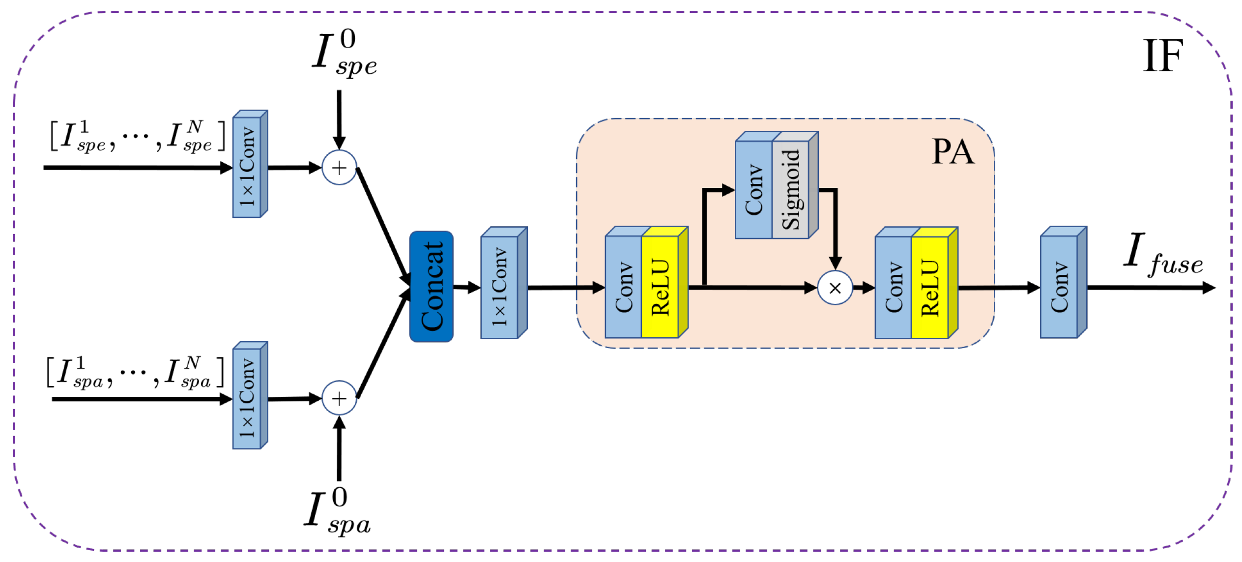
3.5. Information Fusion Module

The main purpose of the information fusion (IF) module is to fuse the interacted spectral-spatial information to reconstruct an HR-MS image $I_{SRMS}$. The schematic of IF is shown in Figure 5.

To fully use the information interacted at different stages, we take as input the concatenation of the spectral and spatial information extracted by each IIG in each branch. First, the concatenated inputs $\left[I_{spe}^1,\cdots ,I_{spe}^N\right]\in {\mathbb{R}}^{H\times W\times NB}$ and $\left[I_{spa}^1,\cdots ,I_{spa}^N\right]\in {\mathbb{R}}^{H\times W\times NB}$ are fed to a $1\times 1$ convolution to squeeze the number of channels, and then the squeezed information is added with its initial extracted spectral $I_{spe}^0$ and spatial $I_{spa}^0$ information to generate feature maps $F_{spe}\in R^{H\times W\times B}$ and $F_{spa}\in R^{H\times W\times B}$, respectively. Next, we concatenate the feature maps in each branch to generate $F_{fuse}\in {\mathbb{R}}^{H\times W\times B}$ and the $1\times 1$ convolution is used for squeeze channels again. This process can be described as:

$$F_{spe}=H_{1\times 1}\left(\left[I_{spe}^1,\cdots ,I_{spe}^N\right]\right)+I_{spe}^0$$

(14)

$$F_{spa}=H_{1\times 1}\left(\left[I_{spa}^1,\cdots ,I_{spa}^N\right]\right)+I_{spa}^0$$

(15)

$$F_{fuse}=H_{1\times 1}\left(\left[F_{spe},F_{spa}\right]\right)$$

(16)

Inspired by [51], we adopt the pixel attention (PA) block at the end of the IF to incorporate the spectral and spatial information, which consists of two convolution layers and a PA layer between them. PA obtains the attention maps, and only goes through a $1\times 1$ convolution and a Sigmoid function, which will then be used to weight the input features. It could effectively improve the final performance at lower parameter cost [51], which is validated by the ablation study in Section 4.4. We denote the proposed PA as $f_{PA}\left(·\right)$, the $F_{fuse}$ is further fed into the PA block:

$$I_{fuse}^{{}^{\prime }}=f_{PA}\left(F_{fuse}\right)$$

(17)

Finally, to match the channel number of the input MS image, a convolutional layer is used to generate the final fusion result:

$$I_{fuse}^{}=H_{3\times 3}\left(I_{fuse}^{{}^{\prime }}\right).$$

(18)

4. Experiments

4.1. Datasets

We conduct experiments using partial datasets provided in [37]. To verify the performance of SSIN, we chose the dataset from three different satellites for our experiments including QuickBird (QB), WorldView-4 (WV4), and WorldView-2 (WV2). The detailed information of the datasets is shown in

Table 1. The detailed information of the datasets.

Satellite Sensors	Image Type	Spatial Dimension	Spectral Dimension	Dimension Size	Bits
QuickBird	MS PAN	2.44 m 0.61 m	Four band one band	256 × 256 × 4 1024 × 1024	11 bit
WorldView4	MS PAN	1.24 m 0.31 m	Four band one band	256 × 256 × 4 1024 × 1024	11 bit
WorldView2	MS PAN	2 m 0.5 m	Eight band one band	256 × 256 × 8 1024 × 1024	11 bit

. For each dataset, we randomly divide the data into the training set and test set by a ratio of 8:2, and twenty percent of the test set is chosen as the validation set. Due to the lack of data volume, the data augmentation is utilized to generate training samples, including random cropping, random horizontal flips, and rotating. After the data augmentation, $400\times 2$, $380\times 2$ and $400\times 2$ image pairs are used as training samples for QB, WV4 and WV2, respectively. The sizes of PAN and LRMS images are $64\times 64$ and $16\times 16$. As for the test data, 80 reduced-scale and 80 full-scale image pairs are utilized. The sizes of reduced-scale PAN and LRMS images are $256\times 256$ and $64\times 64$, respectively. The sizes of full-scale PAN and MS images are $1024\times 1024$ and $256\times 256$, respectively. All the deep learning methods use the same dataset for training and testing.

Following the Wald protocol [52], we downsample the PAN and MS images at a four-fold scale using spatial degradation based on a modulation transfer function (MTF), then we can use the degraded images as the network input and the HR MS images as ground truth image to train the network.

4.2. Train Details

In the training stage, we use the Adam optimization algorithm [53] to optimize our network, and the initial learning rate is set to 0.0005. Every 200 epochs, the learning rate drops by a factor of two. We set the batch size to 10 and the patch size of LRMS images to 16 for training with 1200 epochs. Our network uses the $\ell 1$ norm as the loss function.

In our experiments, all the DL-based approaches are implemented in Pytorch framework and are trained on a GTX-1080Ti GPU, while traditional methods are conducted by MATLAB. As for the test phase, all the objective evaluation indexes are calculated by MATLAB, and the results were averaged on the corresponding test set.

4.3. Evaluation Index

In the reduced-resolution experiment, the HR MS image is usually used as the reference image for evaluation, therefore, commonly used objective evaluation indicators, including spectral angle mapper (SAM) [54], the erreur relative global adimensionnelle de synthese (ERGAS) [55], the correlation coefficient(CC) [56] and the Q2n index [57], is used to evaluate all the approaches at reduced resolution. The optimal values of CC and Q2n are 1, and the best values of for ERGAS and SAM are 0.

Since there is no reference image in the full-resolution experiment, we adopt the popular non-reference quality evaluation index, i.e., the quality with no reference (QNR) [58] to evaluate the pansharpening performance. QNR consists of a spectral distortion index, $D_{\lambda }$ and a spatial distortion index, $D_s$, which can be computed as: $QNR={\left(1-D_{\lambda }\right)}^{\alpha }{\left(1-D_S\right)}^{\beta }$. In the following experiments, $\alpha$ and $\beta$ are both set as to 1. The ideal value is 1 for QNR, and 0 for $D_{\lambda }$ and $D_S$

4.4. Ablation Study

To verify the validity of IIB, SSA, and PA, we conduct an ablation study on the WV2 validation dataset. In this subsection, the number of IIG and the number of RCAB in each IIG are set to four and two, respectively. The results of ablation experiments are given in Table 2. The meanings of each method are as follows:

• Base: Baseline, ablate the PA block, disconnect the interaction cables in each IIB, and removes both spatial and spectral attention from each SSA.
• Base+PA: Add the PA block in IF on the baseline
• Base+PA+SSA: Add both spatial attention and spectral attention on the Base+PA
• Base+PA+SSA+IIB: The method proposed in this paper (SSIN) that turn on the interaction connection in each IIB on the basis of Base+PA+SSA.

For the baseline, we remove PA from IF and turn off the interaction connection in SSA and IIB. By doing this, spatial and spectral information can only be processed separately, and the spatial and spectral branches are independent of each other. From Table 2, it is not hard to see that baseline achieved the worst performance compared to other methods, which illustrates the importance of interaction between the two branches.

Table 2. The quantiative evaluation result of ablation study, the best value is in bold.

Methods	SAM↓	ERGAS↓	Q2n↑	CC↑
Base	3.7354	2.8492	0.7783	0.9634
Base+PA	3.4086	2.605	0.7839	0.968
Base+PA+SSA	3.3495	2.563	0.7854	0.969
Base+PA+SSA+IIB	3.2598	2.4239	0.7882	0.9711

Table 2. The quantiative evaluation result of ablation study, the best value is in bold.

Methods	SAM↓	ERGAS↓	Q2n↑	CC↑
Base	3.7354	2.8492	0.7783	0.9634
Base+PA	3.4086	2.605	0.7839	0.968
Base+PA+SSA	3.3495	2.563	0.7854	0.969
Base+PA+SSA+IIB	3.2598	2.4239	0.7882	0.9711

4.4.1. Effect of the PA

Inspired of [50], we add pixel attention (PA) block in IF to improve information fusion performance. To verify the significance of the PA in the IF. We add the PA in IF based on the baseline, which is called “Base+PA”.

As can be seen in Table 2, compared with baseline, “Base+PA” has significantly improved in all evaluation indexes. The reason is that PA can improve the expression ability of convolutions [50]. In particular, PA can automatically calculate the importance of each neuron in the feature maps for reconstruction according to the input features, and then rescale these neurons with the importance.

4.4.2. Effect of the SSA

To take full advantage of the advantageous information of the spectral branch and spatial branch, we use both spatial attention and spectral attention mechanisms in the SSA module. It can be seen in Table 2 that “Base+PA+SSA” has achieved better fusion performance than “Base+PA”. This is because SSA can make use of the cross-attention mechanism. That is to enhance the spectral characteristics of the spatial branch by spectral attention in the spectral branch, while enhancing spatial characteristics of the spectral branch by using spatial attention of the spatial branch. In this way, the two branches can make up the weakness of each other by using their respective advantages, which are conducive to the final information fusion.

4.4.3. Effect of the IIB

In this section, we assess the effectiveness of the IIB. Comparing “Base+PA+SSA” with “Base+PA+SSA+IIB” in Table 2, we can observe that “Base+PA+SSA”, without any information interaction, has worse results in all objective indicators. This is because SSA can take into account the information from another branch before generating attention. Through the information interaction, the network with SSA can obtain more appropriate and accurate attention weights. Moreover, the spectral-spatial information cannot be effectively incorporated by the IF module without information interactions. With the increase of information interaction, the fusion performance of the network is steadily improved as shown in Figure 6.

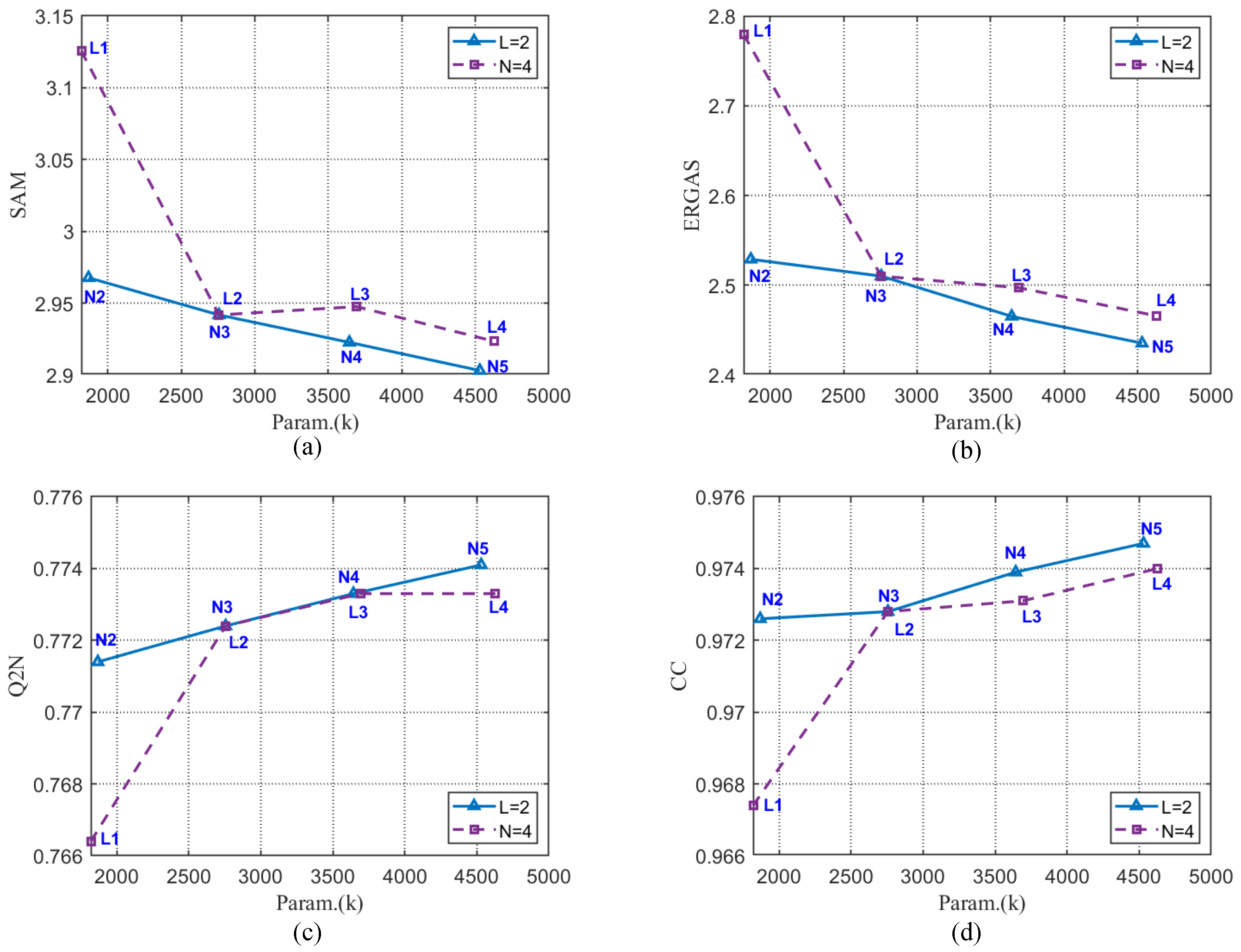
4.5. Parameters Analysis

SSIN is constructed mainly by IIG. The number of IIG, N, and the number of RCAB in each IIG, L, are two key factors affecting network performance.

To explore the impacts of N and L on performance, we conduct eight groups of contrast experiments. In order to keep the number of parameters within a reasonable range, we adjust L from 1 to 4 with a step of 1 by keeping $N=3$, then we adjust N from 2 to 5 with a step of 1 by keeping $L=2$, while the other settings remain unchanged. The experiment is conducted on the WV2 test dataset. The objective evaluation indices results are given in

Table 3. The quantiative evaluation results with different number of IIG and RCAB on the wv2 test dataset. The best value is in bold.

Methods	SAM↓	ERGAS↓	Q2n↑	CC↑	#Params
SSIN (N = 2, L = 2)	2.9677	2.5289	0.7714	0.9726	1.87 M
SSIN (N = 3, L = 2)	2.9418	2.5101	0.7724	0.9728	2.76 M
SSIN (N = 4, L = 2)	2.9227	2.4653	0.7733	0.9739	3.64 M
SSIN (N = 5, L = 2)	2.9031	2.4354	0.7741	0.9747	4.53 M
SSIN (N = 3, L = 1)	3.1256	2.7793	0.7664	0.9674	1.82 M
SSIN (N = 3, L = 2)	2.9418	2.5101	0.7724	0.9728	2.75 M
SSIN (N = 3, L = 3)	2.9476	2.4972	0.7733	0.9731	3.70 M
SSIN (N = 3, L = 4)	2.9234	2.4658	0.7733	0.974	4.63 M

. To obtain the influence of N and L on network performance more intuitively, we show the experimental results in Figure 6.

We first discuss the effect of L with N fixed to 4. The purple curve in Figure 6 shows the experimental results, from which we can find that the SSIN performance and the number of parameters grow with the increase of L, especially when L increase from 1 to 2. However, the increase of L has little impact on network performance when L reaches 2, but brings more parameters. So for the rest of the experiment, the L is set to 2.

Then, we fixed L to 2 to study the effect of N, the results of this part are shown by the blue curve in Figure 6. As we can see, with the increase of N, the performance and the number of parameters of SSIN increase steadily, especially in Figure 6a,c. This is because the number of IIB grows as N increases, and information interaction can enhance the performance of the SSA module and significantly improve the final information fusion performance, as we discussed in Section 4.4.

In addition, it is worth noting that increasing N can bring greater performance improvement than increasing L under the condition of a similar number of parameters. The main reason is that increase of L can enhance the ability of information extraction but hinder the dissemination of information, while the increase of N can significantly increase the number of information interactions. The interaction between spectral information and spatial information has a more important impact on the performance of SSIN.

To sum up, considering the performance and the number of parameters, we selected $N=4$ and $L=2$ as our final setting for our proposed SSIN.

4.6. Comparison with SOTA Methods

In this section, to verify the effectiveness of SSIN, several SOTA pansharpening methods are used to conduct comparative experiments at both reduced resolution and full resolution. For a fair comparison, all parameters of the DL-based approach are kept consistent with the original papers for best performance. In this article we use an implementation of traditional methods that can be downloaded for free [23,59].

The SOTA pansharpening methods used for comparison includes the MS image interpolation (EXP) [34], the robust band-dependent spatial detail (BDSD-PC) [60], GS adaptive (GSA) [28], partial replacement adaptive CS (PRACS) [29], MTF-GLP [61], and seven DL-based methods, such as PNN [6], PanNet [7], MSDCNN [12], TFNET [13], GGPCRN [45], MUCNN [15], MDA-Net [46].

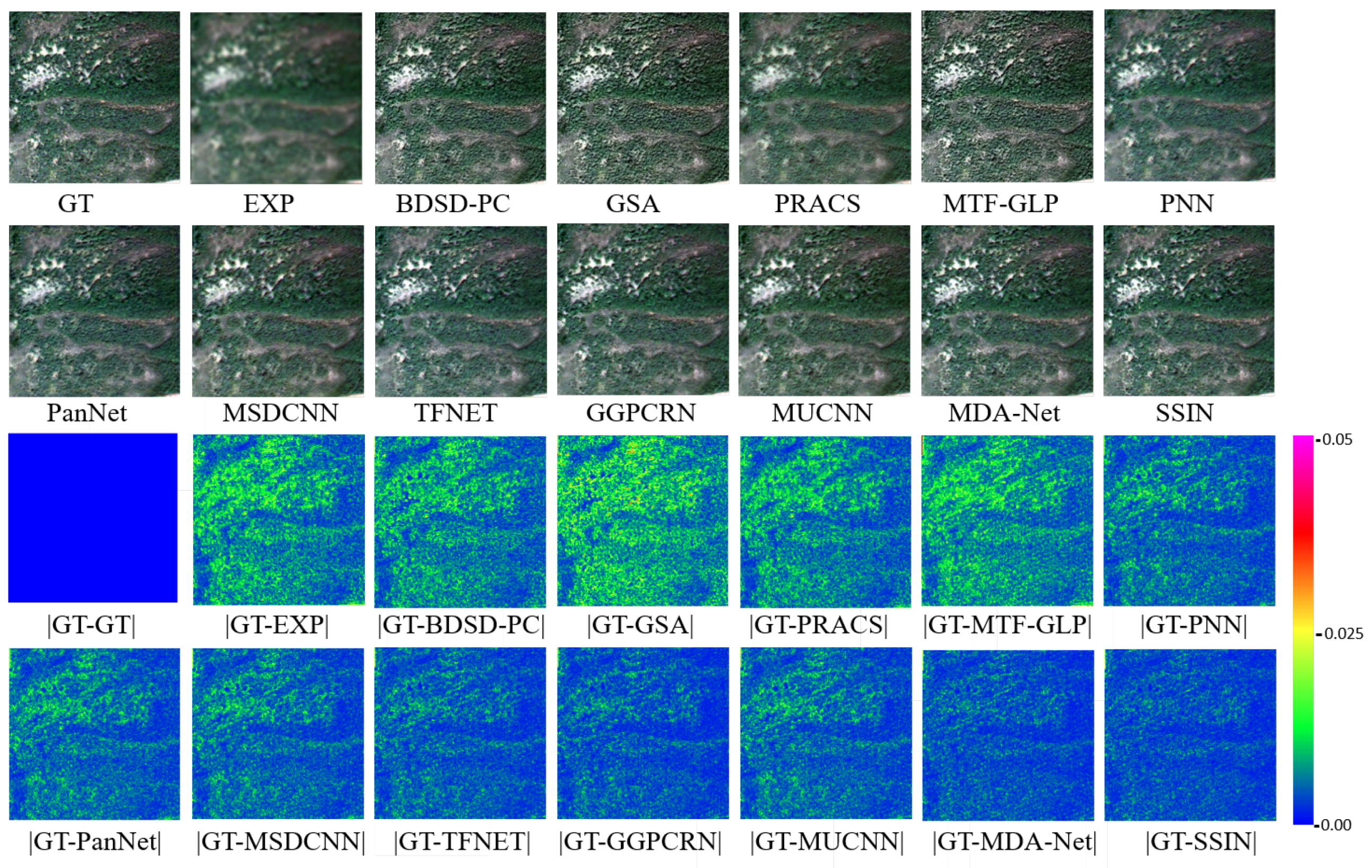
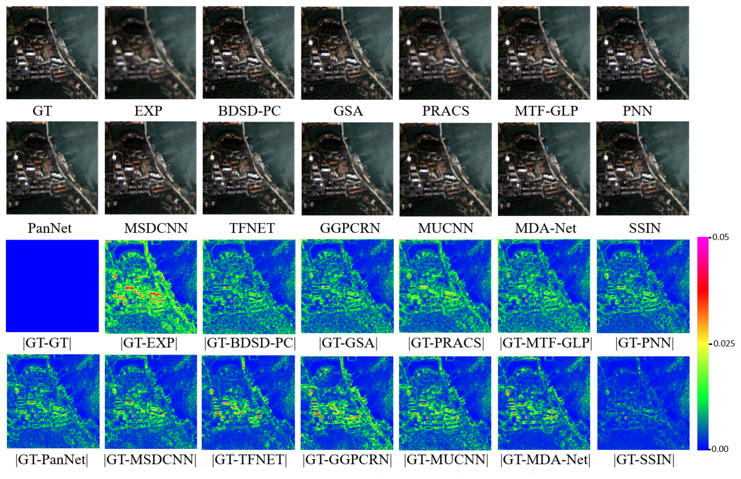
4.6.1. Reduced-Resolution Experiments

The reduced-resolution experimental results of different methods on the QB datasets sets are shown in

Table 4. Quantiative results of different methods on the QB dataset. The best results are in bold and the second-best results are underlined.

Methods	SAM↓	ERGAS↓	Q2N↑	CC↑
EXP	1.8768	1.8316	0.6913	0.8776
GSA	1.4291	1.1440	0.8329	0.9447
PRACS	1.4681	1.1957	0.8210	0.9406
BDSD-PC	1.4268	1.1099	0.8388	0.9470
MTF-GLP	1.4162	1.1602	0.8282	0.9438
PNN	1.1802	0.9451	0.8660	0.9601
PanNet	1.0350	0.8068	0.8825	0.9686
MSDCNN	1.0011	0.7787	0.8830	0.9696
TFNET	0.8475	0.6494	0.8991	0.9778
GGPCRN	0.7714	0.5951	0.9091	0.9809
MUCNN	0.9134	0.7121	0.8950	0.9737
MDA-Net	0.7740	0.5908	0.9104	0.9815
SSIN	0.7292	0.5427	0.914	0.9833

. It can be clearly observed from Table 4 that DL-based methods outperform the traditional methods on the evaluation indexes, which reflect the powerful fusion performance of deep learning. Among them, our proposed SSIN performs the best for all the reduced-resolution indexes, followed by MDA-Net [46], which demonstrates the effectiveness of SSIN. Similar results also appear on WV4 and WV2 datasets, as shown in

Table 5. Quantiative evaluation comparison of different methods on the WV4 dataset. The best results are in bold and the second-best results are underlined.

Methods	SAM↓	ERGAS↓	Q2N↑	CC↑
EXP	2.5639	3.2561	0.6957	0.9026
GSA	2.6454	2.5375	0.7735	0.9372
PRACS	2.5875	2.4452	0.7753	0.9412
BDSD-PC	2.6018	2.4424	0.7876	0.9435
MTF-GLP	2.5785	2.5715	0.7783	0.9409
PNN	1.9677	1.9709	0.8371	0.9583
PanNet	1.9605	1.9341	0.8361	0.9594
MSDCNN	1.8648	1.8522	0.8492	0.9618
TFNET	1.4589	1.3066	0.8909	0.9788
GGPCRN	1.3167	1.1445	0.9025	0.9826
MUCNN	1.7308	1.7138	0.8676	0.9675
MDA-Net	1.3068	1.1487	0.9040	0.9828
SSIN	1.1994	1.0399	0.9095	0.9853

and

Table 6. Quantiative evaluation comparison of different methods on the WV2 dataset. The best results are in bold and the second-best results are underlined.

Methods	SAM↓	ERGAS↓	Q2N↑	CC↑
EXP	5.3078	7.3730	0.4887	0.8017
GSA	4.9165	5.0016	0.6764	0.9089
PRACS	5.1933	5.8450	0.6111	0.8844
BDSD-PC	4.8530	4.7933	0.6853	0.9169
MTF-GLP	4.7501	4.8380	0.6899	0.9150
PNN	3.7671	3.4542	0.7422	0.9535
PanNet	3.6355	3.2757	0.7545	0.9574
MSDCNN	3.4789	3.0815	0.7528	0.9608
TFNET	3.1212	2.6381	0.7642	0.9702
GGPCRN	3.0029	2.5669	0.7699	0.9715
MUCNN	3.3052	2.9356	0.7576	0.9642
MDA-Net	2.9554	2.5030	0.7737	0.9729
SSIN	2.9227	2.4653	0.7733	0.9739

. SSIN achieves the best result except the Q2n on WV2.

Although the quantitative evaluation shows the excellent performance of SSIN, in order to demonstrate the effect of SSIN in subjective evaluation, we make a subjective visual comparison of some samples in the above datasets. To prove the universality of SSIN, we selected images of three different scenes from the above datasets for comparison. Specifically, the harbor image is from the QB dataset, the forest image is from the WV4 dataset, and the city image is from the WV2 dataset.

Figure 7, Figure 8 and Figure 9 present the visual comparison of different methods on the three satellite datasets. For intuitive comparison, residual results between fusion image and the ground truth are also presented. The concrete method is to take the average of the absolute values of each band residuals.

Figure 7 displays the fusion results of an image from the QB dataset. We can clearly see from Figure 7 that the results of EXP and PRACS methods are blurred and contain serious spatial distortion compared with GT. The results of the BDSD-PC, PNN, and MUCNN are slightly darker than the ground truth (GT). According to the residual result from Figure 7, it can be found that the error between the traditional method and the GT is greater, while the DL-based methods have less error. Moreover, comparing various DL-based methods, we can see that our proposed SSIN is the closest to the GT, which indicates that our model has better performance in spatial recovery and spectral preservation.

A visual comparison of WV4 dataset is shown in Figure 8. As can be seen, EXP, PRACS, PNN, and MSDCNN produce very blurry images with serious spatial distortion, while the results of BDSD-PC, GSA, and MTF-GLP generate significant spectral distortion in the forest area. The results of the MDA-Net, GGPCRN and our proposed methods are difficult to discern visually. We can further see the residual result from Figure 8, similarly to the experimental results of the QB dataset case, DL-based methods are closer to GT than traditional methods. Among DL-based methods, the residual image of MDA-Net and SSIN is closer to GT than others, which is consistent with the results of the quantitative evaluation shown in Table V. Although the residual image of MDA-Net is very close to that of SSIN, further observation reveals that MDA-Net is slightly brighter than SSIN.

The visual comparison of the WV2 dataset is depicted in Figure 9. It can be observed that, compared with the first two datasets, the test results of each method have larger errors in the WV2 dataset. The reason is that the number of bands in the WV2 dataset is twice that of the first two datasets, making reconstruction more difficult. This can also be seen by comparing objective indicators of the three datasets. As we can see from the residual result in Figure 8, the results of the proposed SSIN are closer to the GT. In particular, it can be clearly seen from the circle in the upper right corner of the residual image that SSIN has the smallest error.

The above comparison at reduced resolution demonstrates the superior performance of SSIN.

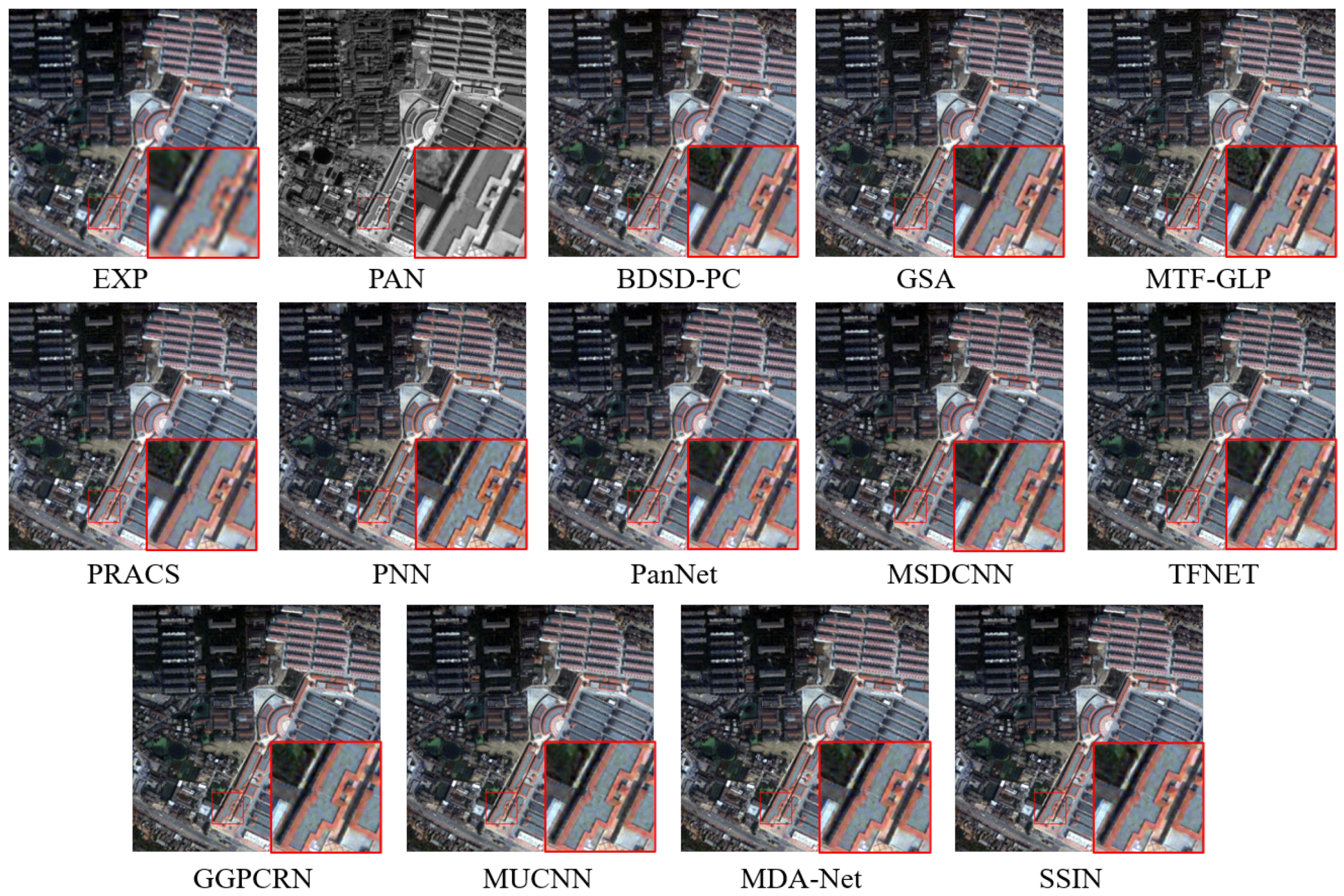
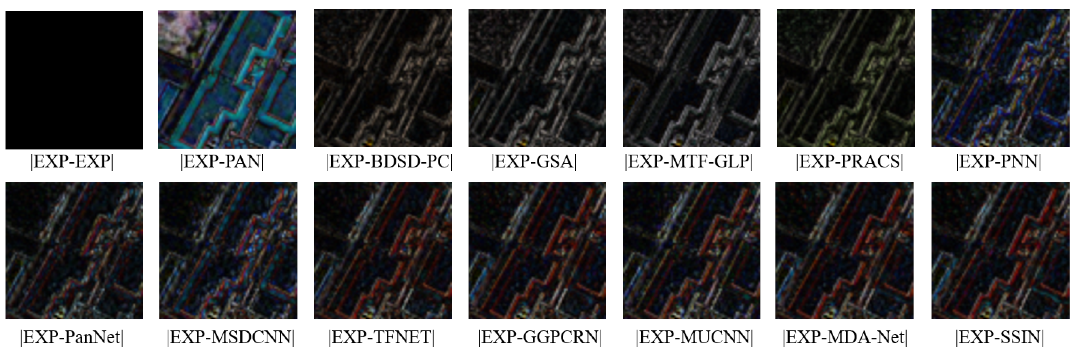
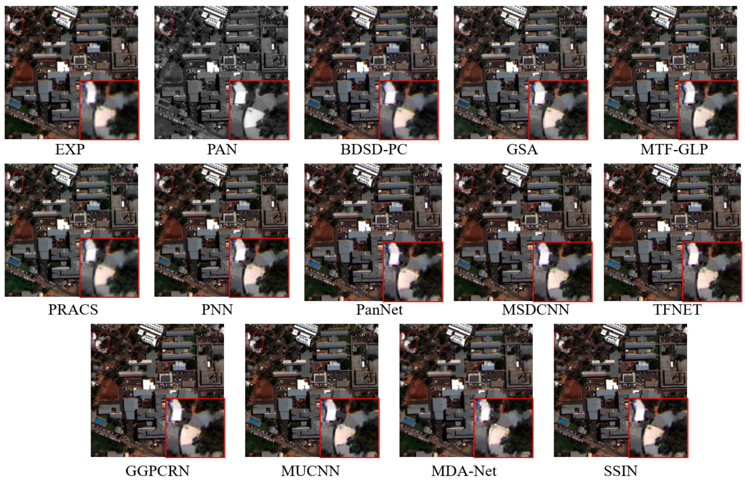
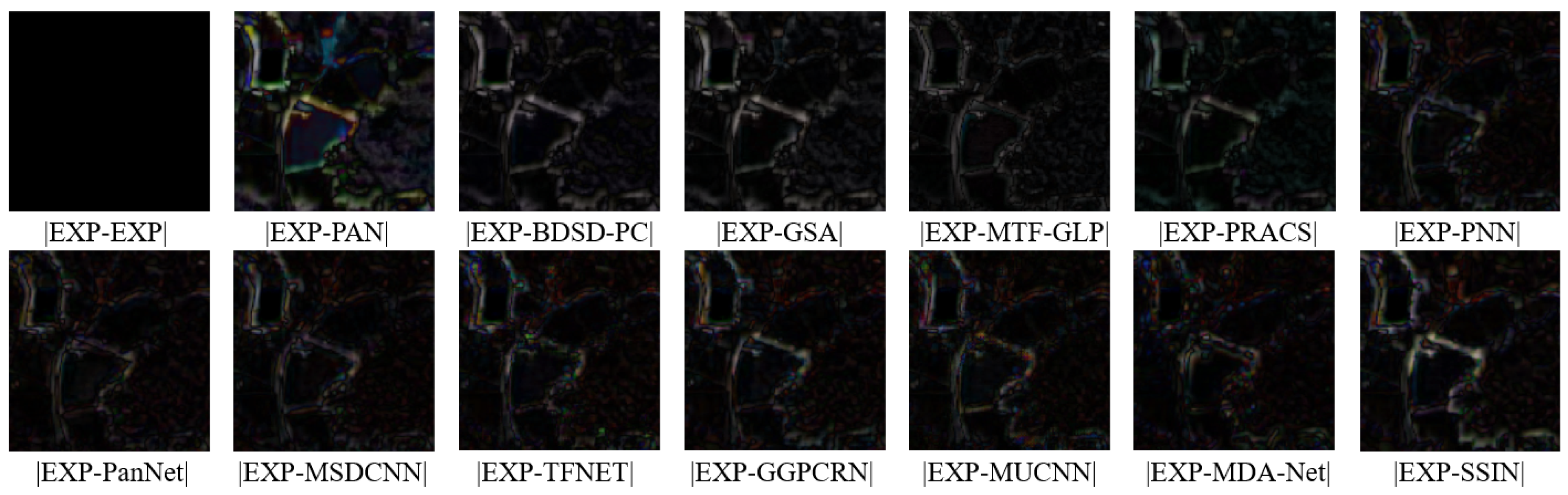
4.6.2. Full-Resolution Experiments

In order to evaluate the generality of the above method, we also conducted a full-resolution experiment on the QB and WV4 datasets. Table 7 shows the average quantitative results of the full-resolution experiments from the QB and WV4 datasets. Since the EXP does not inject the details of the PAN image into the LRMS image, the result of the EXP shows spectral features similar to those of the LRMS image, which can be regarded as a reference for evaluating spectral preservation [9,59] and excluded from the comparison.

As shown in Table 7, our method is mediocre in $D_{\lambda }$ on both QB and WV4 datasets but achieves the best results in $D_s$ and the QNR of our method is high, which demonstrated our method still achieves satisfactory fusion results. One potential reason is that the spatial attention of SSA module changes the spectral features excessively during the interaction process, resulting in the reduction of the fidelity of the original spectral information.

Table 7. Quantitative evaluation comparison of different methods on the QB and WV4 dataset at the full-resolution experiments. The best results are in bold and the second-best results are underlined.

Methods	QB			WV4
	${\mathit{D}}_{\mathit{\lambda }}$↓	${\mathit{D}}_{\mathit{s}}$↓	QNR↑	${\mathit{D}}_{\mathit{\lambda }}$↓	${\mathit{D}}_{\mathit{s}}$↓	QNR↑
EXP	0	0.1016	0.8984	0	0.0819	0.9181
GSA	0.0875	0.1743	0.7584	0.0766	0.1576	0.7803
PRACS	0.0465	0.1096	0.8510	0.0305	0.0975	0.8758
BDSD-PC	0.0622	0.1515	0.7998	0.0478	0.1258	0.8350
MTF-GLP	0.1261	0.2004	0.7056	0.0914	0.1332	0.7907
PNN	0.0622	0.1115	0.8374	0.0473	0.0612	0.8944
PanNet	0.0604	0.0990	0.8502	0.0326	0.0620	0.9076
MSDCNN	0.0572	0.1025	0.8493	0.0449	0.0665	0.8927
TFNET	0.0492	0.0728	0.8840	0.0569	0.0562	0.8905
GGPCRN	0.0509	0.0688	0.8858	0.0555	0.0581	0.8902
MUCNN	0.0488	0.0886	0.86	0.0611	0.0591	0.8847
MDA-Net	0.0473	0.0656	0.8921	0.0560	0.0607	0.8873
SSIN	0.0532	0.0609	0.8910	0.0483	0.0534	0.9012

Table 7. Quantitative evaluation comparison of different methods on the QB and WV4 dataset at the full-resolution experiments. The best results are in bold and the second-best results are underlined.

Methods	QB			WV4
	${\mathit{D}}_{\mathit{\lambda }}$↓	${\mathit{D}}_{\mathit{s}}$↓	QNR↑	${\mathit{D}}_{\mathit{\lambda }}$↓	${\mathit{D}}_{\mathit{s}}$↓	QNR↑
EXP	0	0.1016	0.8984	0	0.0819	0.9181
GSA	0.0875	0.1743	0.7584	0.0766	0.1576	0.7803
PRACS	0.0465	0.1096	0.8510	0.0305	0.0975	0.8758
BDSD-PC	0.0622	0.1515	0.7998	0.0478	0.1258	0.8350
MTF-GLP	0.1261	0.2004	0.7056	0.0914	0.1332	0.7907
PNN	0.0622	0.1115	0.8374	0.0473	0.0612	0.8944
PanNet	0.0604	0.0990	0.8502	0.0326	0.0620	0.9076
MSDCNN	0.0572	0.1025	0.8493	0.0449	0.0665	0.8927
TFNET	0.0492	0.0728	0.8840	0.0569	0.0562	0.8905
GGPCRN	0.0509	0.0688	0.8858	0.0555	0.0581	0.8902
MUCNN	0.0488	0.0886	0.86	0.0611	0.0591	0.8847
MDA-Net	0.0473	0.0656	0.8921	0.0560	0.0607	0.8873
SSIN	0.0532	0.0609	0.8910	0.0483	0.0534	0.9012

Figure 10 and Figure 11 show the visualized results of different methods on QB and WV4 datasets in the full-resolution experiment, respectively. In addition, we enlarge the region marked in the red box in the fused images for better subjective evaluation. To intuitively observe the differences between different methods, the residual image between the results of EXP and the results of other methods in Figure 10 and Figure 11 are shown in Figure 12 and Figure 13, respectively.

As shown in Figure 10, The results of PNN, PanNet, and MSDCNN suffer from obvious spectral distortion. The results of BDSD-PC, GSA, MTF-GLP, and PRACS yield different levels of spatial distortion compared with the PAN. Specifically, they produce thicker strip structures. The other methods produce better visual results. From the residual images in Figure 12, we can see that the traditional methods inject fewer details than the compared DL-based methods but have better spectral preservation. On the DL based category, we can find that the residual image of PNN, PanNet, and MSDCNN has obvious spatial distortion. Because there are noise pixels in the whole residual image, however, the residual images of the rest of the methods are difficult to discriminate.

Figure 10. The full-resolution experiments results of different methods on QB dataset.

Figure 10. The full-resolution experiments results of different methods on QB dataset.

Figure 11. The full-resolution experiments results of different methods on WV4 dataset.

Figure 11. The full-resolution experiments results of different methods on WV4 dataset.

Figure 11 shows results of a full-resolution sample from WV4. As it shows, the result of the GSA and PRACS exhibits serious spectral distortion. Specifically, the grass color in the lower-left corner of the result images is lighter than the result of EXP. The results of the BDSD-PC, MTF-GLP, and PRACS are blurred and present serious spatial distortion. As for DL-based methods, MSDCNN, MUCNN, PanNet, PNN, TFNET, and MDA-Net produce obvious artifacts and spatial distortion with varying degrees. GGPCRN and SSIN generate relatively clearer images. As shown in the enlarged area, we can observe that the results of PNN, PanNet, TFNET, MUCNN, and MDA-Net contain obvious spectral distortions evidenced by distinct color pixels from the result of EXP. As we can see in Figure 13, MTF-GLP and BDSD-PC inject fewer details than DL-based methods. However, GSA injects more details than PNN, PanNet, MSDCNN, and MDA-Net. PRACS observably injects the spatial details, but there is significant spectral distortion, as the residual image of PRACS is obvious color deviation. Furthermore, the residual images of PNN, PanNet, MSDCNN, TFNET, MUCNN, MDA-Net, and SSIN exhibit different levels of spectral distortion as the residual images have many distinct colors of pixels. Although our SSIN suffers from some spectral distortion and is slightly worse than BDSD-PC, GSA, and MTF-GLP in spectral preservation, it injects more edges into the fusion result.

Figure 12. Residual results of the enlarged region of Figure 10.

Figure 12. Residual results of the enlarged region of Figure 10.

Figure 13. Residual results of the enlarged region of Figure 11.

Figure 13. Residual results of the enlarged region of Figure 11.

Overall, from the above results of both reduced- and full-resolution experiments, our SSIN achieves favorable and promising performance in spatial detail injection and spectral preservation.

5. Efficiency Study

In order to compare the computational time and learnable parameters of different methods, we record the results of different methods on the full-resolution experiments from WV4 datasets as shown in

Table 8. Performance comparison of different methods.

	Methods	Time(s)	#Parameters
Traditional methods	EXP	0.1136	-
	BDSD-PC	0.199	-
	GSA	0.5937	-
	PRACS	0.97	-
	MTF-GLP	0.4555	-
DL-based methods	PNN	0.008	80 K
	PanNet	0.009	77 k
	MSDCNN	0.0089	190 K
	TFNET	0.0095	2.36 M
	GGPCRN	0.014	1.77 M
	MUCNN	0.0081	1.36 M
	MDA-Net	0.0172	12 M
	SSIN	0.0157	3.63 M

. All traditional methods are implemented using MATLAB and tested on an Intel Core i7-12700K CPU. DL-based methods are tested on a desktop with an Nvidia RTX 3090 GPU. As shown in Table 8, the traditional methods take more computational time than the DL-based methods. PRACS is the slowest method, whose computational time is about 1s per image. As for DL-based methods, although MDA-Net has achieved good results in previous experiments, it needs more time and computational cost to generate the fused images. Although SSIN has a slightly larger number of parameters than other DL-based methods except for MDA-Net, it has better performance.

6. Conclusions

In this paper, we proposed a dual-branch network named SSIN with spectral-spatial interaction for pansharpening. In the proposed SSIN, the PAN and the LRMS images are processed separately to fully extract their features. SSIN extracted spatial information from the PAN image and spectral information from the MS image. To make the most of the spatial-spectral information, we propose an information interaction block based on a dual-branch network to promote the interaction between spectral and spatial information. Furthermore, the spectral-spatial attention module is used to guide information integration and enhance the characteristics of the another branch. The performance improvement of the two modules for the dual-branch network was proved in the ablation study. Moreover, we used pixel attention in the information fusion module to adjust the importance of each pixel in the feature maps, thereby further improving the network performance. Extensive experiments have demonstrated the effectiveness of our proposed method on pansharpening.

References

1. Meng, X.; Shen, H.; Li, H.; Zhang, L.; Fu, R. Review of the pansharpening methods for remote sensing images based on the idea of meta-analysis: Practical discussion and challenges. Inf. Fusion 2019, 46, 102–113. [Google Scholar] [CrossRef]
2. Gilbertson, J.K.; Kemp, J.; van Niekerk, A. Effect of pan-sharpening multi-temporal Landsat 8 imagery for crop type differentiation using different classification techniques. Comput. Electron. Agric. 2017, 134, 151–159. [Google Scholar] [CrossRef] [Green Version]
3. Du, P.; Liu, S.; Xia, J.; Zhao, Y. Information fusion techniques for change detection from multi-temporal remote sensing images. Inf. Fusion 2013, 14, 19–27. [Google Scholar] [CrossRef]
4. Qu, Y.; Qi, H.; Ayhan, B.; Kwan, C.; Kidd, R. DOES multispectral/hyperspectral pansharpening improve the performance of anomaly detection? In Proceedings of the 2017 IEEE International Geoscience and Remote Sensing Symposium (IGARSS), Fort Worth, TX, USA, 23–28 July 2017; pp. 6130–6133. [Google Scholar] [CrossRef]
5. Dong, C.; Loy, C.C.; He, K.; Tang, X. Learning a Deep Convolutional Network for Image Super-Resolution. In Proceedings of the Computer Vision—ECCV 2014; Fleet, D., Pajdla, T., Schiele, B., Tuytelaars, T., Eds.; Springer International Publishing: Cham, Switzerland, 2014; pp. 184–199. [Google Scholar]
6. Masi, G.; Cozzolino, D.; Verdoliva, L.; Scarpa, G. Pansharpening by Convolutional Neural Networks. Remote Sens. 2016, 8, 594. [Google Scholar] [CrossRef] [Green Version]
7. Yang, J.; Fu, X.; Hu, Y.; Huang, Y.; Ding, X.; Paisley, J. PanNet: A Deep Network Architecture for Pan-Sharpening. In Proceedings of the 2017 IEEE International Conference on Computer Vision (ICCV), Venice, Italy, 22–29 October 2017; pp. 1753–1761. [Google Scholar] [CrossRef]
8. Wei, Y.; Yuan, Q. Deep residual learning for remote sensed imagery pansharpening. In Proceedings of the 2017 International Workshop on Remote Sensing with Intelligent Processing (RSIP), Shanghai, China, 18–21 May 2017; pp. 1–4. [Google Scholar] [CrossRef]
9. Chen, L.; Lai, Z.; Vivone, G.; Jeon, G.; Chanussot, J.; Yang, X. ArbRPN: A Bidirectional Recurrent Pansharpening Network for Multispectral Images With Arbitrary Numbers of Bands. IEEE Trans. Geosci. Remote Sens. 2022, 60, 1–18. [Google Scholar] [CrossRef]
10. Lei, D.; Chen, H.; Zhang, L.; Li, W. NLRNet: An Efficient Nonlocal Attention ResNet for Pansharpening. IEEE Trans. Geosci. Remote. Sens. 2022, 60, 1–13. [Google Scholar] [CrossRef]
11. Li, C.; Zheng, Y.; Jeon, B. Pansharpening via Subpixel Convolutional Residual Network. IEEE J. Sel. Top. Appl. Earth Obs. Remote. Sens. 2021, 14, 10303–10313. [Google Scholar] [CrossRef]
12. Yuan, Q.; Wei, Y.; Meng, X.; Shen, H.; Zhang, L. A multiscale and multidepth convolutional neural network for remote sensing imagery pan-sharpening. IEEE J. Sel. Top. Appl. Earth Obs. Remote Sens. 2018, 11, 978–989. [Google Scholar] [CrossRef] [Green Version]
13. Liu, X.; Liu, Q.; Wang, Y. Remote sensing image fusion based on two-stream fusion network. Inf. Fusion 2020, 55, 1–15. [Google Scholar] [CrossRef] [Green Version]
14. Yang, Y.; Tu, W.; Huang, S.; Lu, H.; Wan, W.; Gan, L. Dual-Stream Convolutional Neural Network With Residual Information Enhancement for Pansharpening. IEEE Trans. Geosci. Remote Sens. 2022, 60, 1–16. [Google Scholar] [CrossRef]
15. Wang, Y.; Deng, L.J.; Zhang, T.J.; Wu, X. SSconv: Explicit Spectral-to-Spatial Convolution for Pansharpening. In Proceedings of the 29th ACM International Conference on Multimedia, Virtual Event, 20–24 October 2021; pp. 4472–4480. [Google Scholar]
16. Fu, S.; Meng, W.; Jeon, G.; Chehri, A.; Zhang, R.; Yang, X. Two-Path Network with Feedback Connections for Pan-Sharpening in Remote Sensing. Remote Sens. 2020, 12, 1674. [Google Scholar] [CrossRef]
17. Zhong, X.; Qian, Y.; Liu, H.; Chen, L.; Wan, Y.; Gao, L.; Qian, J.; Liu, J. Attention FPNet: Two-Branch Remote Sensing Image Pansharpening Network Based on Attention Feature Fusion. IEEE J. Sel. Top. Appl. Earth Obs. Remote Sens. 2021, 14, 11879–11891. [Google Scholar] [CrossRef]
18. Wu, X.; Huang, T.Z.; Deng, L.J.; Zhang, T.J. Dynamic Cross Feature Fusion for Remote Sensing Pansharpening. In Proceedings of the IEEE/CVF International Conference on Computer Vision (ICCV), Montreal, BC, Canada, 11–17 October 2021; pp. 14687–14696. [Google Scholar]
19. Yao, J.; Hong, D.; Chanussot, J.; Meng, D.; Zhu, X.; Xu, Z. Cross-Attention in Coupled Unmixing Nets for Unsupervised Hyperspectral Super-Resolution. In Proceedings of the Computer Vision—ECCV 2020; Vedaldi, A., Bischof, H., Brox, T., Frahm, J.M., Eds.; Springer International Publishing: Cham, Switzerland, 2020; pp. 208–224. [Google Scholar]
20. Kim, J.; Lee, J.K.; Lee, K.M. Accurate Image Super-Resolution Using Very Deep Convolutional Networks. In Proceedings of the IEEE Conference on Computer Vision and Pattern Recognition (CVPR), Las Vegas, NV, USA, 27–30 June 2016. [Google Scholar]
21. Lim, B.; Son, S.; Kim, H.; Nah, S.; Mu Lee, K. Enhanced Deep Residual Networks for Single Image Super-Resolution. In Proceedings of the IEEE Conference on Computer Vision and Pattern Recognition (CVPR) Workshops, Honolulu, HI, USA, 21–26 July 2017. [Google Scholar]
22. Ledig, C.; Theis, L.; Huszar, F.; Caballero, J.; Cunningham, A.; Acosta, A.; Aitken, A.; Tejani, A.; Totz, J.; Wang, Z.; et al. Photo-Realistic Single Image Super-Resolution Using a Generative Adversarial Network. In Proceedings of the IEEE Conference on Computer Vision and Pattern Recognition (CVPR), Honolulu, HI, USA, 21–26 July 2017. [Google Scholar]
23. Vivone, G.; Dalla Mura, M.; Garzelli, A.; Restaino, R.; Scarpa, G.; Ulfarsson, M.O.; Alparone, L.; Chanussot, J. A new benchmark based on recent advances in multispectral pansharpening: Revisiting pansharpening with classical and emerging pansharpening methods. IEEE Geosci. Remote Sens. Mag. 2020, 9, 53–81. [Google Scholar] [CrossRef]
24. Haydn, R. Application of the IHS color transform to the processing of multisensor data and image enhancement. In Proceedings of the International Symposium on Remote Sensing of Arid and Semi-Arid Lands, Cairo, Egypt, 19–25 January 1982. [Google Scholar]
25. Carper, W.; Lillesand, T.; Kiefer, R. The use of intensity-hue-saturation transformations for merging SPOT panchromatic and multispectral image data. Photogramm. Eng. Remote Sens. 1990, 56, 459–467. [Google Scholar]
26. Kwarteng, P.; Chavez, A. Extracting spectral contrast in Landsat Thematic Mapper image data using selective principal component analysis. Photogramm. Eng. Remote Sens. 1989, 55, 339–348. [Google Scholar]
27. Laben, C.A.; Brower, B.V. Process for Enhancing the Spatial Resolution of Multispectral Imagery Using Pan-Sharpening. U.S. Patent 6,011,875, 4 January 2000. [Google Scholar]
28. Aiazzi, B.; Baronti, S.; Selva, M. Improving component substitution pansharpening through multivariate regression of MS + Pan data. IEEE Trans. Geosci. Remote Sens. 2007, 45, 3230–3239. [Google Scholar] [CrossRef]
29. Choi, J.; Yu, K.; Kim, Y. A new adaptive component-substitution-based satellite image fusion by using partial replacement. IEEE Trans. Geosci. Remote Sens. 2010, 49, 295–309. [Google Scholar] [CrossRef]
30. Garzelli, A.; Nencini, F.; Capobianco, L. Optimal MMSE Pan Sharpening of Very High Resolution Multispectral Images. IEEE Trans. Geosci. Remote Sens. 2008, 46, 228–236. [Google Scholar] [CrossRef]
31. Ghassemian, H. A review of remote sensing image fusion methods. Inf. Fusion 2016, 32, 75–89. [Google Scholar] [CrossRef]
32. Pradhan, P.S.; King, R.L.; Younan, N.H.; Holcomb, D.W. Estimation of the number of decomposition levels for a wavelet-based multiresolution multisensor image fusion. IEEE Trans. Geosci. Remote Sens. 2006, 44, 3674–3686. [Google Scholar] [CrossRef]
33. Burt, P.J.; Adelson, E.H. The Laplacian pyramid as a compact image code. In Readings in Computer Vision; Elsevier: Amsterdam, The Netherlands, 1987; pp. 671–679. [Google Scholar]
34. Aiazzi, B.; Alparone, L.; Baronti, S.; Garzelli, A. Context-driven fusion of high spatial and spectral resolution images based on oversampled multiresolution analysis. IEEE Trans. Geosci. Remote Sens. 2002, 40, 2300–2312. [Google Scholar] [CrossRef]
35. Shah, V.P.; Younan, N.H.; King, R.L. An efficient pan-sharpening method via a combined adaptive PCA approach and contourlets. IEEE Trans. Geosci. Remote Sens. 2008, 46, 1323–1335. [Google Scholar] [CrossRef]
36. Yang, Y.; Lu, H.; Huang, S.; Tu, W. Pansharpening based on joint-guided detail extraction. IEEE J. Sel. Top. Appl. Earth Obs. Remote Sens. 2020, 14, 389–401. [Google Scholar] [CrossRef]
37. Meng, X.; Xiong, Y.; Shao, F.; Shen, H.; Sun, W.; Yang, G.; Yuan, Q.; Fu, R.; Zhang, H. A large-scale benchmark data set for evaluating pansharpening performance: Overview and implementation. IEEE Geosci. Remote Sens. Mag. 2020, 9, 18–52. [Google Scholar] [CrossRef]
38. Mascarenhas, N.; Banon, G.; Candeias, A. Multispectral image data fusion under a Bayesian approach. Int. J. Remote Sens. 1996, 17, 1457–1471. [Google Scholar] [CrossRef]
39. Ballester, C.; Caselles, V.; Igual, L.; Verdera, J.; Rougé, B. A variational model for P+ XS image fusion. Int. J. Comput. Vis. 2006, 69, 43–58. [Google Scholar] [CrossRef]
40. Meng, X.; Shen, H.; Yuan, Q.; Li, H.; Zhang, L.; Sun, W. Pansharpening for cloud-contaminated very high-resolution remote sensing images. IEEE Trans. Geosci. Remote Sens. 2018, 57, 2840–2854. [Google Scholar] [CrossRef]
41. Zhang, L.; Shen, H.; Gong, W.; Zhang, H. Adjustable model-based fusion method for multispectral and panchromatic images. IEEE Trans. Syst. Man Cybern. Part (Cybern.) 2012, 42, 1693–1704. [Google Scholar] [CrossRef]
42. Li, S.; Yang, B. A new pan-sharpening method using a compressed sensing technique. IEEE Trans. Geosci. Remote Sens. 2010, 49, 738–746. [Google Scholar] [CrossRef]
43. Zhu, X.X.; Bamler, R. A sparse image fusion algorithm with application to pan-sharpening. IEEE Trans. Geosci. Remote Sens. 2012, 51, 2827–2836. [Google Scholar] [CrossRef]
44. Lai, Z.; Chen, L.; Jeon, G.; Liu, Z.; Zhong, R.; Yang, X. Real-time and effective pan-sharpening for remote sensing using multi-scale fusion network. J.-Real-Time Image Process. 2021, 18, 1635–1651. [Google Scholar] [CrossRef]
45. Lai, Z.; Chen, L.; Liu, Z.; Yang, X. Gradient Guided Pyramidal Convolution Residual Network with Interactive Connections for Pan-sharpening. Int. J. Remote. Sens. 2021, 1–31. [Google Scholar] [CrossRef]
46. Guan, P.; Lam, E.Y. Multistage Dual-Attention Guided Fusion Network for Hyperspectral Pansharpening. IEEE Trans. Geosci. Remote. Sens. 2022, 60, 1–14. [Google Scholar] [CrossRef]
47. Wang, Y.; Wang, L.; Yang, J.; An, W.; Yu, J.; Guo, Y. Spatial-angular interaction for light field image super-resolution. In Proceedings of the European Conference on Computer Vision, Glasgow, UK, 23–28 August 2020; pp. 290–308. [Google Scholar]
48. Zhang, Y.; Li, K.; Li, K.; Wang, L.; Zhong, B.; Fu, Y. Image super-resolution using very deep residual channel attention networks. In Proceedings of the European Conference on Computer Vision (ECCV), Munich, Germany, 8–14 September 2018; pp. 286–301. [Google Scholar]
49. Glorot, X.; Bordes, A.; Bengio, Y. Deep sparse rectifier neural networks. In Proceedings of the 14th International Conference on Artificial Intelligence and Statistics. JMLR Workshop and Conference Proceedings, Ft. Lauderdale, FL, USA, 11–13 April 2011; pp. 315–323. [Google Scholar]
50. Wang, Q.; Wu, B.; Zhu, P.; Li, P.; Hu, Q. ECA-Net: Efficient Channel Attention for Deep Convolutional Neural Networks. In Proceedings of the 2020 IEEE/CVF Conference on Computer Vision and Pattern Recognition (CVPR), Seattle, WA, USA, 13–19 June 2020. [Google Scholar]
51. Zhao, H.; Kong, X.; He, J.; Qiao, Y.; Dong, C. Efficient image super-resolution using pixel attention. In Proceedings of the European Conference on Computer Vision, Glasgow, UK, 23–28 August 2020; pp. 56–72. [Google Scholar]
52. Wald, L.; Ranchin, T.; Mangolini, M. Fusion of satellite images of different spatial resolutions: Assessing the quality of resulting images. Photogramm. Eng. Remote Sens. 1997, 63, 691–699. [Google Scholar]
53. Kingma, D.P.; Ba, J. Adam: A method for stochastic optimization. arXiv 2014, arXiv:1412.6980. [Google Scholar]
54. Yuhas, R.H.; Goetz, A.F.; Boardman, J.W. Discrimination among semi-arid landscape endmembers using the spectral angle mapper (SAM) algorithm. In Proceedings of the JPL, Summaries of the Third Annual JPL Airborne Geoscience Workshop, Pasadena, CA, USA, 1–5 June 1992. [Google Scholar]
55. Wald, L. Data Fusion: Definitions and Architectures: Fusion of Images of Different Spatial Resolutions; Presses des MINES: Paris, France, 2002. [Google Scholar]
56. Palsson, F.; Sveinsson, J.R.; Benediktsson, J.A.; Aanaes, H. Classification of pansharpened urban satellite images. IEEE J. Sel. Top. Appl. Earth Obs. Remote. Sens. 2011, 5, 281–297. [Google Scholar] [CrossRef]
57. Garzelli, A.; Nencini, F. Hypercomplex quality assessment of multi/hyperspectral images. IEEE Geosci. Remote. Sens. Lett. 2009, 6, 662–665. [Google Scholar] [CrossRef]
58. Alparone, L.; Aiazzi, B.; Baronti, S.; Garzelli, A.; Nencini, F.; Selva, M. Multispectral and panchromatic data fusion assessment without reference. Photogramm. Eng. Remote. Sens. 2008, 74, 193–200. [Google Scholar] [CrossRef] [Green Version]
59. Vivone, G.; Alparone, L.; Chanussot, J.; Dalla Mura, M.; Garzelli, A.; Licciardi, G.A.; Restaino, R.; Wald, L. A critical comparison among pansharpening algorithms. IEEE Trans. Geosci. Remote. Sens. 2014, 53, 2565–2586. [Google Scholar] [CrossRef]
60. Vivone, G. Robust band-dependent spatial-detail approaches for panchromatic sharpening. IEEE Trans. Geosci. Remote Sens. 2019, 57, 6421–6433. [Google Scholar] [CrossRef]
61. Aiazzi, B.; Alparone, L.; Baronti, S.; Garzelli, A.; Selva, M. MTF-tailored multiscale fusion of high-resolution MS and Pan imagery. Photogramm. Eng. Remote Sens. 2006, 72, 591–596. [Google Scholar] [CrossRef]
Figure 1. The architecture of the proposed SSIN.
Remotesensing 14 04100 g001
Figure 2. Schematic diagram of the information interaction group, “⊕” denotes elementwise addition, and “⊗” denotes matrix multiplication.
Remotesensing 14 04100 g002
Figure 3. Schematic diagram of the information interaction block, “⊕”denotes elementwise addition, and “⊗” denotes matrix multiplication.
Remotesensing 14 04100 g003
Figure 4. Schematic diagram of the spectral-spatial attention module, “⊕” denotes elementwise addition, and “⊗” denotes matrix multiplication.
Remotesensing 14 04100 g004
Figure 5. Schematic diagram of the information fusion module, “⊕” denotes elementwise addition, and “⊗” denotes matrix multiplication.
Remotesensing 14 04100 g005
Figure 6. Compare network performance and parameters configured with different parameters. (a) the result of SAM. (b) the result of ERGAS. (c) the result of Q2n. (d) the result of CC.
Remotesensing 14 04100 g006
Figure 7. The reduced-resolution experiments results of different methods on QB dataset.
Remotesensing 14 04100 g007
Figure 8. The reduced-resolution experiments results of different methods on WV4 dataset.
Remotesensing 14 04100 g008
Figure 9. The reduced-resolution experiments results of different methods on WV2 dataset.
Remotesensing 14 04100 g009