
Uniform and Competency-Based 3D Keypoint Detection for Coarse Registration of Point Clouds with Homogeneous Structure


Abstract
:
1. Introduction
2. Related Works
2.1. Keypoint Detectors 3DSIFT and 3DISS
2.2. Keypoint Descriptor SHOT
2.3. Limiations of Current Approaches
2.3.1. Measures for Keypoint Quality
- 3D Local Shape Features
- 3D Self Similarity
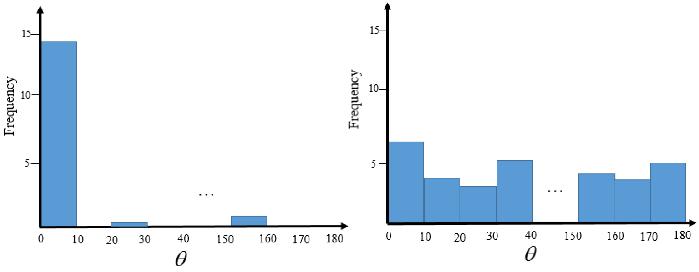
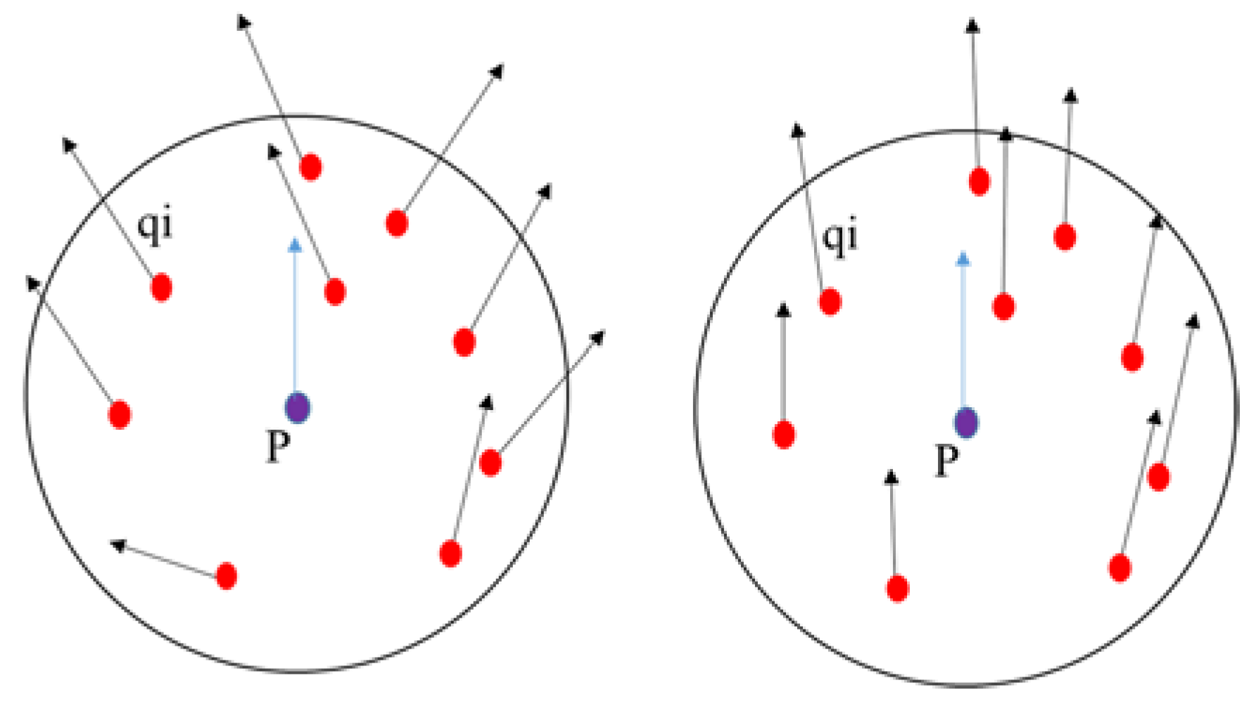
- Histogram of Normal Orientations
2.3.2. Spatial Distribution and the Number of Keypoints
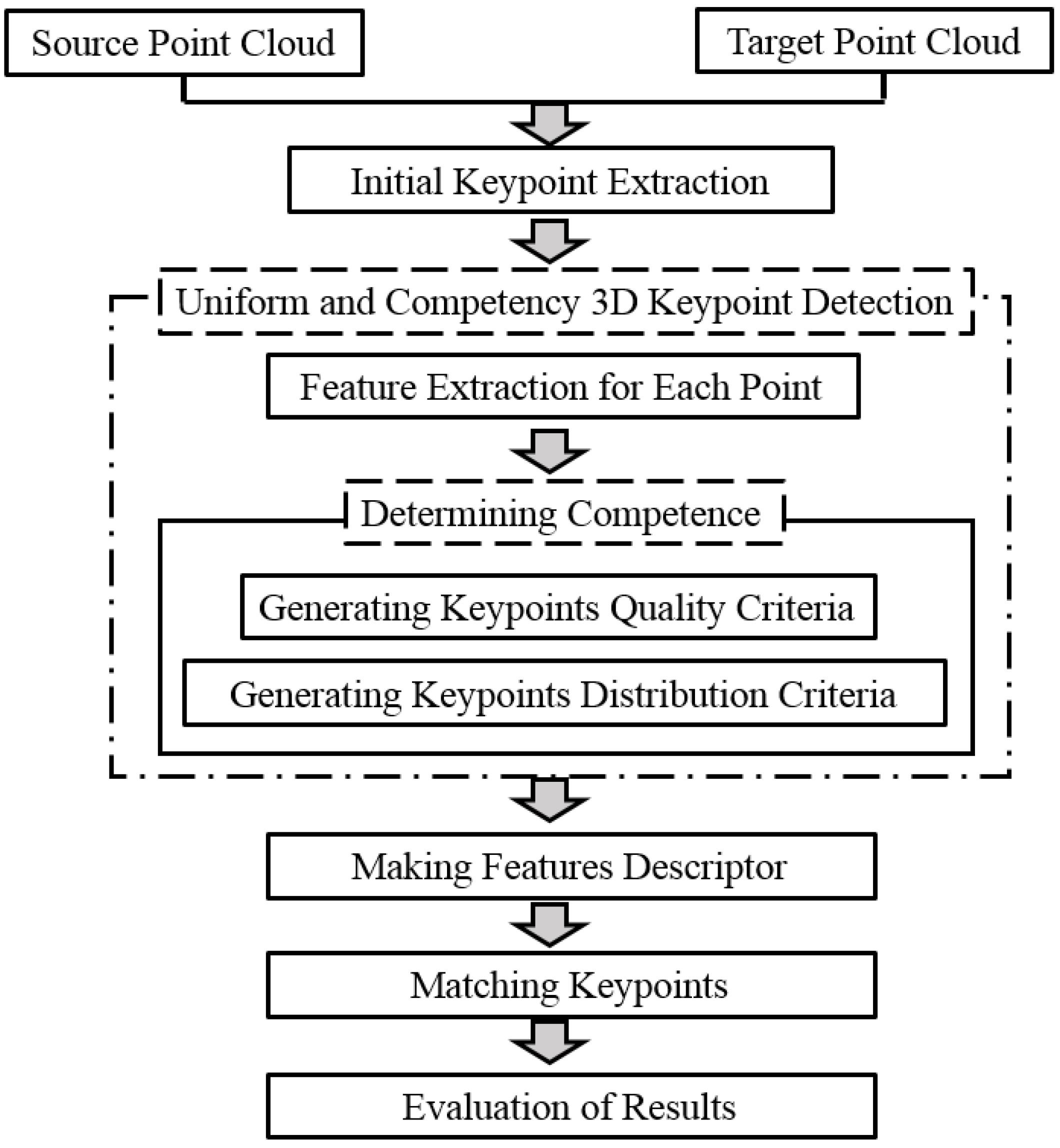
3. Proposed Method
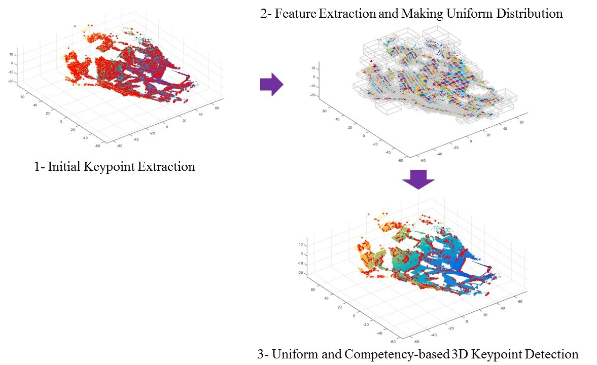
- Extraction of initial keypoints by detector algorithms (3DSIFT or 3DISS). At this stage, by selecting small thresholds, a relatively large number of points are extracted.
- Estimate competence for each initial keypoint by:
- (1)
- The 3D shape features (Scattering, omnivariance, anisotropy, change of curvature), the 3D self-similarity feature, and the Histogram of Normal Orientations feature are extracted for each initial keypoint. These properties are considered as a vector with n components as follows:where i is related to the initial point number and j is for the criteria number (m is equal to 6 here).
- (2)
- The ranking vector of the initial points is determined for each criterion. The highest value will be the first rank, and the lowest value will be the last rank for all criteria except anisotropy (Aλ). The criterion anisotropy is the opposite, and the lowest value will have the highest rank. The ranking vector of each criterion is displayed as follows:where is related to the keypoint in the criterion vector and indicates the rank of this keypoint against others in that criterion.
- (3)
- The competence of initial keypoints is calculated using a combination of all criteria as follows:where corresponds to the competence of the kepoints, indicates the rank of the kepoints in the criterion, n is equal to the number of keypoints, m is the number of criteria. is the weight parameter for the criterion, which is used to control the effect of different criteria on the keypoints quality. The sum of the weights of the various criteria must be equal to one. The higher the C-competence criterion is, the better the complication is, and it has more probabilities of success in the matching process.
- 3.
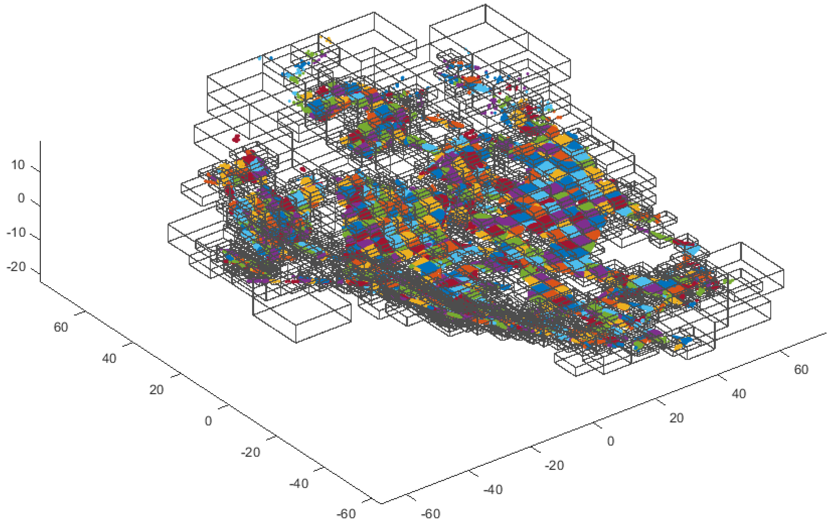
- The control of the keypoint spatial distribution is conducted by cell formation in point clouds based on the Octree structure. The details of this process are as follows:
- (1)
- The point cloud space is cellularized using the Octree structure. Using the depth parameter, it is determined to what extent the cell formation will continue.
- (2)
- The total number of required keypoints (N) is determined for detection. The N parameter controls the number of required keypoints for extraction.
- (3)
- The number of extractable keypoints in each cell is calculated according to the value of competence and the number of initial points located in each cell. In fact, in this step, it is determined how many of the total numbers of required keypoints (parameter N) are allocated to each cell. This process is determined as follows:where is the number of initial keypoints located in a specific cell and represents the average competency of the keypoints in that cell. wn and wc are weights related to and . In general, the higher the number of initial keypoints in a cell and the higher the average competency of the keypoints, the more points are extracted from that cell.
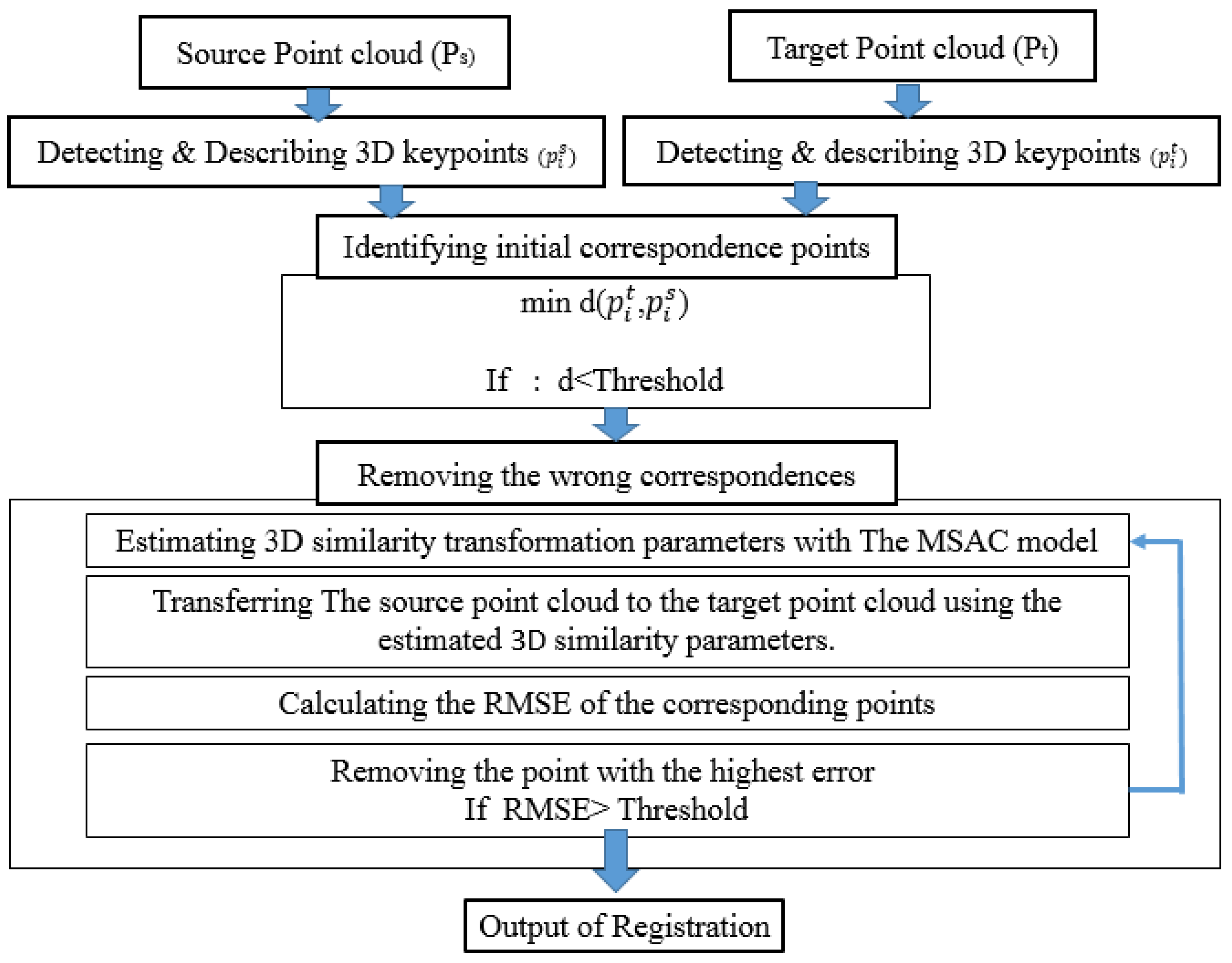
3.1. Matching and Registration
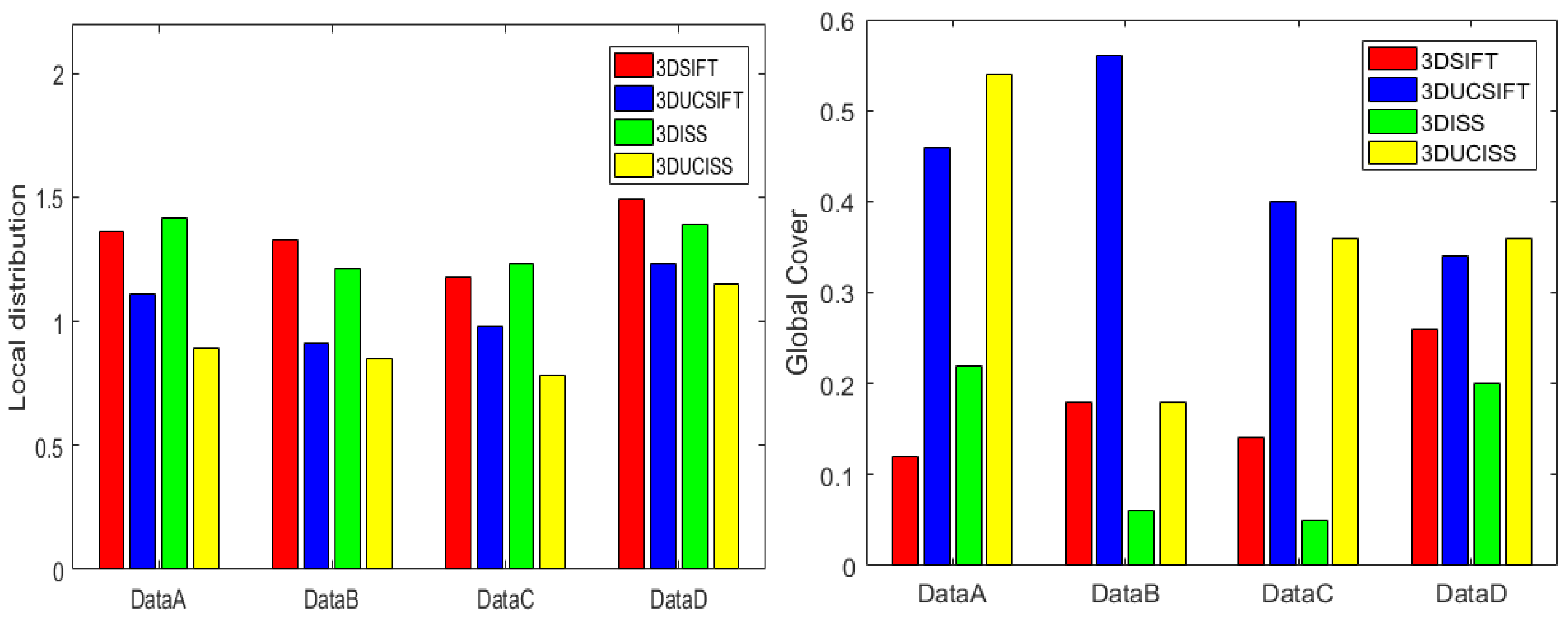
3.2. Evaluation Criteria
4. Experiments
4.1. Data
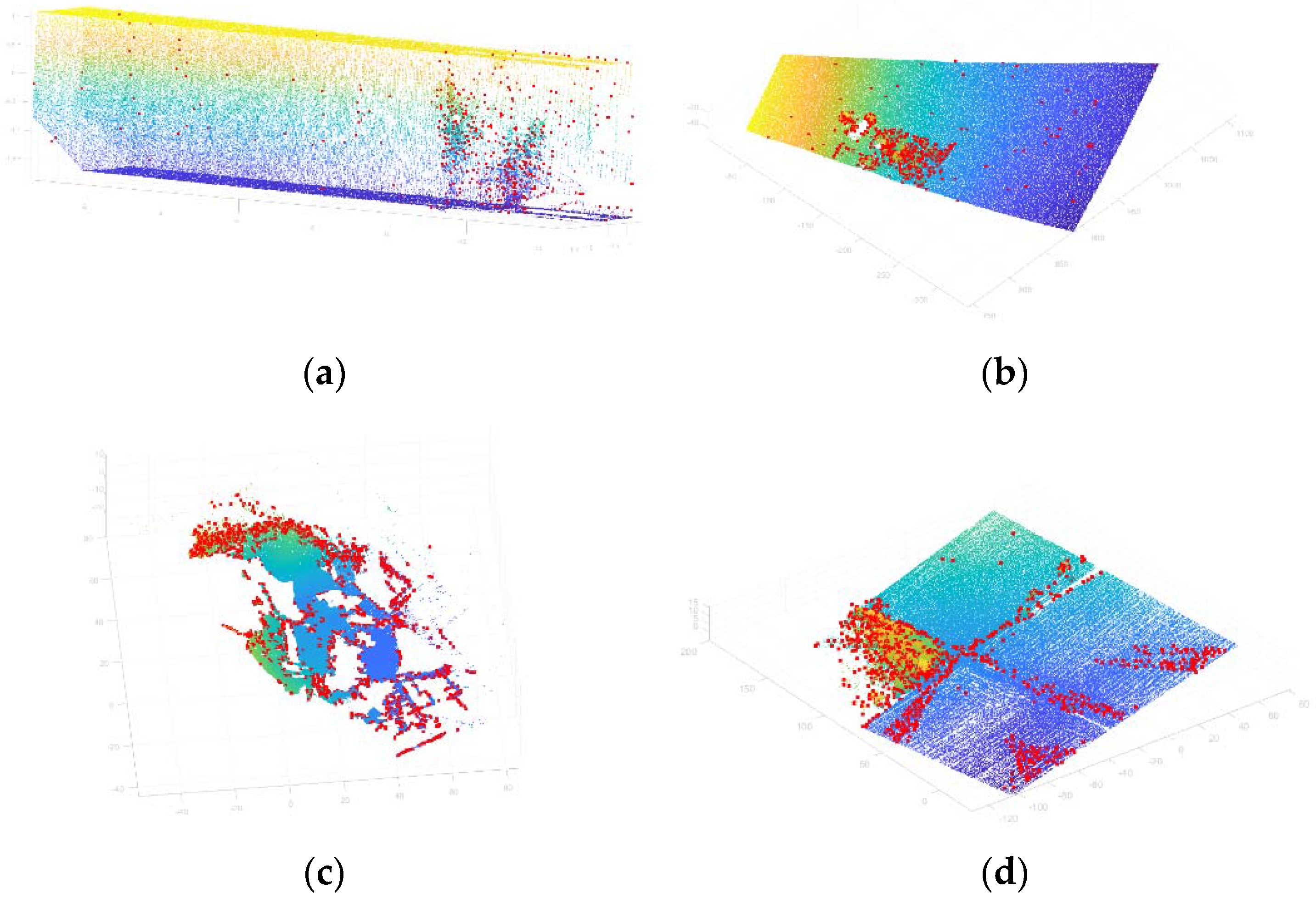
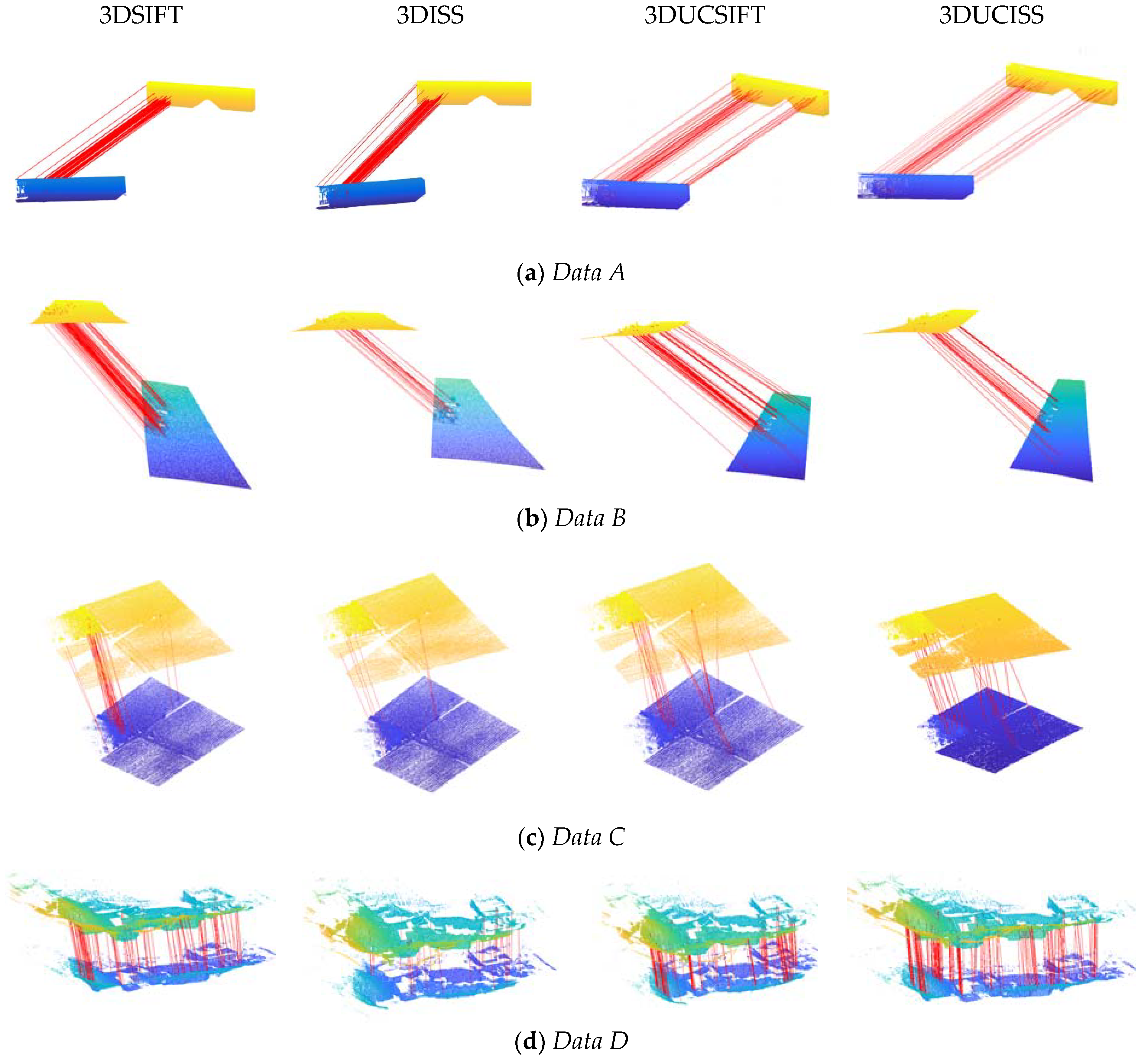
- Data A: These data were obtained by terrestrial laser scanner in an indoor environment at two different stations with 100% coverage. They were taken from a corridor of a university building (TU Wien). In Figure 8a, we can see some objects concentrated in a small area of the corridor, and there are also some installed signs along the corridor.
- Data B: This point cloud was obtained using aerial laser scanners at Ranzenbach (a forested area in lower Austria, west of Vienna). It was provided by the company Riegl and acquired in April 2021. The used scanner in this data is VQ-1560 II-S. The scan area consists of a flat area in the middle and a forest of different tree types around it. The selected area included a small section of dense trees, and other areas had an almost homogeneous surface. The secondary data were simulated to create the co-registration conditions. The simulated data were generated by applying shifts, rotations, and density changes in the point cloud to examine the co-registration process.
- Data C: These data were taken by Terrestrial laser scanners in an outdoor environment at two different stations with 100% coverage. The geographical location of the data is in the flat, rural area of Vienna (22nd district). These data can be divided into three parts. The first part consists of dense trees. The second part consists of flat land, and the third part includes agricultural land with little topographic changes.
- Data D: These data are a subset of the ETH PRS TLS benchmark as the Courtyard dataset. Point clouds in this benchmark were taken by a Z + F Imager 5006i and Faro Focus 3D and provided in an outdoor environment for the TLS point cloud registration. There are no vertical objects in these data. It was generated to create DTMs.
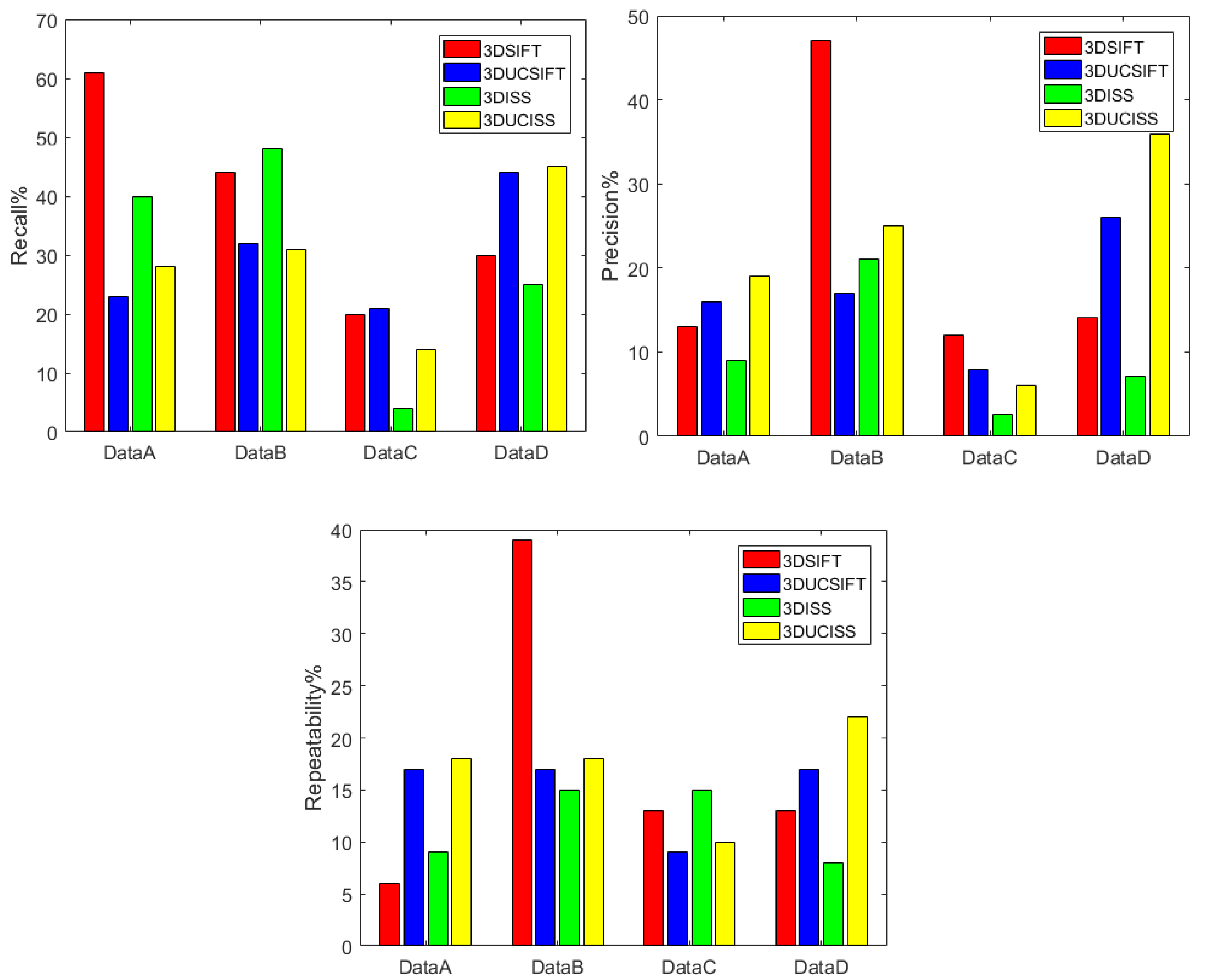
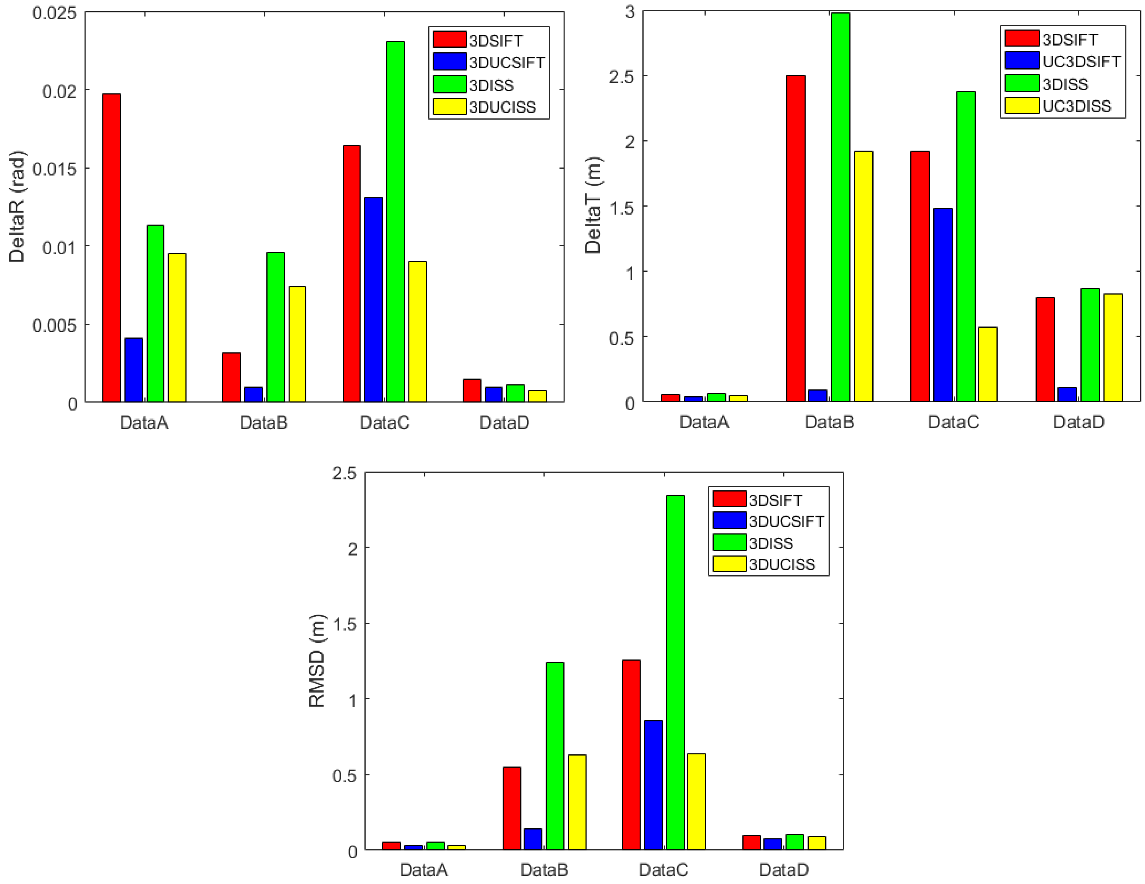
4.2. Results
5. Conclusions and Suggestions
Author Contributions
Funding
Data Availability Statement
Acknowledgments
Conflicts of Interest
References
- Li, W.; Cheng, H.; Zhang, X. Efficient 3D Object Recognition from Cluttered Point Cloud. Sensors 2021, 21, 5850. [Google Scholar] [CrossRef] [PubMed]
- Cheng, Q.; Sun, P.; Yang, C.; Yang, Y.; Liu, P.X. A morphing-Based 3D point cloud reconstruction framework for medical image processing. Comput. Methods Programs Biomed. 2020, 193, 105495. [Google Scholar] [CrossRef] [PubMed]
- Liang, X.; Hyyppä, J.; Kaartinen, H.; Lehtomäki, M.; Pyörälä, J.; Pfeifer, N.; Holopainen, M.; Brolly, G.; Francesco, P.; Hackenberg, J.; et al. International benchmarking of terrestrial laser scanning approaches for forest inventories. ISPRS J. Photogramm. Remote Sens. 2018, 144, 137–179. [Google Scholar] [CrossRef]
- Milenković, M.; Pfeifer, N.; Glira, P. Applying terrestrial laser scanning for soil surface roughness assessment. Remote Sens. 2015, 7, 2007–2045. [Google Scholar] [CrossRef] [Green Version]
- Theiler, P.W.; Wegner, J.D.; Schindler, K. Keypoint-based 4-points congruent sets–automated marker-less registration of laser scans. ISPRS J. Photogramm. Remote Sens. 2014, 96, 149–163. [Google Scholar] [CrossRef]
- Besl, P.J.; McKay, N.D. Method for registration of 3-D shapes. In Proceedings of the Sensor Fusion IV: Control Paradigms and Data Structures, Boston, MA, USA, 14–15 November 1991. [Google Scholar]
- Glira, P.; Pfeifer, N.; Briese, C.; Ressl, C. A correspondence framework for ALS strip adjustments based on variants of the ICP algorithm. Photogramm. Fernerkund. Geoinf. 2015, 4, 275–289. [Google Scholar] [CrossRef]
- Yang, J.; Cao, Z.; Zhang, Q. A fast and robust local descriptor for 3D point cloud registration. Inf. Sci. 2016, 346, 163–179. [Google Scholar] [CrossRef]
- Salti, S.; Tombari, F.; di Stefano, L. A performance evaluation of 3d keypoint detectors. In Proceedings of the 2011 International Conference on 3D Imaging, Modeling, Processing, Visualization and Transmission, Hangzhou, China, 16–19 May 2011. [Google Scholar]
- Shah, S.A.A.; Bennamoun, M.; Boussaid, F. Keypoints-based surface representation for 3D modeling and 3D object recognition. Pattern Recognit. 2017, 64, 29–38. [Google Scholar] [CrossRef]
- Tang, J.; Ericson, L.; Folkesson, J.; Jensfelt, P. GCNv2: Efficient correspondence prediction for real-time SLAM. IEEE Robot. Autom. Lett. 2019, 4, 3505–3512. [Google Scholar] [CrossRef] [Green Version]
- Nie, W.; Xiang, S.; Liu, A. Multi-scale CNNs for 3D model retrieval. Multimed. Tools Appl. 2018, 77, 22953–22963. [Google Scholar] [CrossRef]
- Wang, Y.; Yang, B.; Chen, Y.; Liang, F.; Dong, Z. JoKDNet: A joint keypoint detection and description network for large-scale outdoor TLS point clouds registration. Int. J. Appl. Earth Obs. Geoinf. 2021, 104, 102534. [Google Scholar]
- Yoshiki, T.; Kanji, T.; Naiming, Y. Scalable change detection from 3d point cloud maps: Invariant map coordinate for joint viewpoint-change localization. In Proceedings of the 2018 21st International Conference on Intelligent Transportation Systems (ITSC), Maui, HI, USA, 4–7 November 2018. [Google Scholar]
- Tombari, F.; Salti, S.; di Stefano, L. Performance evaluation of 3D keypoint detectors. Int. J. Comput. Vis. 2013, 102, 198–220. [Google Scholar] [CrossRef]
- Chen, H.; Bhanu, B. 3D free-form object recognition in range images using local surface patches. Pattern Recognit. Lett. 2007, 28, 1252–1262. [Google Scholar] [CrossRef]
- Zhong, Y. Intrinsic shape signatures: A shape descriptor for 3d object recognition. In Proceedings of the 2009 IEEE 12th International Conference on Computer Vision Workshops, ICCV Workshops, Kyoto, Japan, 27 September–4 October 2009. [Google Scholar]
- Mian, A.; Bennamoun, M.; Owens, R. On the repeatability and quality of keypoints for local feature-based 3d object retrieval from cluttered scenes. Int. J. Comput. Vis. 2010, 89, 348–361. [Google Scholar] [CrossRef] [Green Version]
- Fiolka, T.; Stückler, J.; Klein, D.A.; Schulz, D.; Behnke, S. Sure: Surface entropy for distinctive 3d features. In International Conference on Spatial Cognition; Springer: Berlin/Heidelberg, Germany, 2012. [Google Scholar]
- Sipiran, I.; Bustos, B. Harris 3D: A robust extension of the Harris operator for interest point detection on 3D meshes. Vis. Comput. 2011, 27, 963–976. [Google Scholar] [CrossRef]
- Castellani, U.; Cristani, M.; Fantoni, S.; Murino, V. Sparse points matching by combining 3D mesh saliency with statistical descriptors. In Computer Graphics Forum; Wiley Online Library: Hoboken, NJ, USA, 2008. [Google Scholar]
- Zaharescu, A.; Boyer, E.; Varanasi, K.; Horaud, R. Surface feature detection and description with applications to mesh matching. In Proceedings of the 2009 IEEE Conference on Computer Vision and Pattern Recognition, Miami, FL, USA, 20–25 June 2009. [Google Scholar]
- Donoser, M.; Bischof, H. 3d segmentation by maximally stable volumes (msvs). In Proceedings of the 18th International Conference on Pattern Recognition (ICPR’06), Hong Kong, China, 20–24 August 2006. [Google Scholar]
- Rusu, R.B.; Cousins, S. 3d is here: Point cloud library (pcl). In Proceedings of the 2011 IEEE International Conference on Robotics and Automation, Shanghai, China, 9–13 May 2011. [Google Scholar]
- Persad, R.A.; Armenakis, C. Automatic co-registration of 3D multi-sensor point clouds. ISPRS J. Photogramm. Remote Sens. 2017, 130, 162–186. [Google Scholar] [CrossRef]
- Weinmann, M.; Weinmann, M.; Hinz, S.; Jutzi, B. Fast and automatic image-based registration of TLS data. ISPRS J. Photogramm. Remote Sens. 2011, 66, S62–S70. [Google Scholar] [CrossRef]
- Petricek, T.; Svoboda, T. Point cloud registration from local feature correspondences—Evaluation on challenging datasets. PLoS ONE 2017, 12, e0187943. [Google Scholar] [CrossRef] [Green Version]
- Bueno, M.; González-Jorge, H.; Martínez-Sánchez, J.; Lorenzo, H. Automatic point cloud coarse registration using geometric keypoint descriptors for indoor scenes. Autom. Constr. 2017, 81, 134–148. [Google Scholar] [CrossRef]
- Zhu, J.; Xu, Y.; Hoegner, L.; Stilla, U. Direct co-registration of TIR images and MLS point clouds by corresponding keypoints. ISPRS Ann. Photogramm. Remote Sens. Spat. Inf. Sci. 2019, 4, 235–242. [Google Scholar] [CrossRef] [Green Version]
- Tonioni, A.; Salti, S.; Tombari, F.; Spezialetti, R.; Stefano, L.D. Learning to detect good 3D keypoints. Int. J. Comput. Vis. 2018, 126, 1–20. [Google Scholar] [CrossRef]
- Teran, L.; Mordohai, P. 3D interest point detection via discriminative learning. In European Conference on Computer Vision; Springer: Berlin/Heidelberg, Germany, 2014. [Google Scholar]
- Alcantarilla, P.F.; Bartoli, A.; Davison, A.J. KAZE features. In European Conference on Computer Vision; Springer: Berlin/Heidelberg, Germany, 2012. [Google Scholar]
- Salti, S.; Tombari, F.; Spezialetti, R.; Di Stefano, L. Learning a descriptor-specific 3D keypoint detector. In Proceedings of the IEEE International Conference on Computer Vision, Washington, DC, USA, 7–13 December 2015. [Google Scholar]
- Godil, A.; Wagan, A.I. Salient local 3D features for 3D shape retrieval. In Three-Dimensional Imaging, Interaction, and Measurement; SPIE: Bellingham, MA, USA, 2011. [Google Scholar]
- Hänsch, R.; Weber, T.; Hellwich, O. Comparison of 3D interest point detectors and descriptors for point cloud fusion. ISPRS Ann. Photogramm. Remote Sens. Spat. Inf. Sci. 2014, 2, 57. [Google Scholar] [CrossRef] [Green Version]
- Lowe, D.G. Distinctive image features from scale-invariant keypoints. Int. J. Comput. Vis. 2004, 60, 91–110. [Google Scholar] [CrossRef]
- Salti, S.; Tombari, F.; di Stefano, L. SHOT: Unique signatures of histograms for surface and texture description. Comput. Vis. Image Underst. 2014, 125, 251–264. [Google Scholar]
- Hana, X.F.; Jin, J.S.; Xie, J.; Wang, M.J.; Jiang, W. A comprehensive review of 3D point cloud descriptors. arXiv 2018, arXiv:1802.02297. [Google Scholar]
- Weinmann, M. Reconstruction and Analysis of 3D Scenes; Springer: Berlin/Heidelberg, Germany, 2016. [Google Scholar]
- Huang, J.; You, S. Point cloud matching based on 3D self-similarity. In Proceedings of the 2012 IEEE Computer Society Conference on Computer Vision and Pattern Recognition Workshops, Providence, RI, USA, 16–21 June 2012. [Google Scholar]
- Prakhya, S.M.; Liu, B.; Lin, W. Detecting keypoint sets on 3D point clouds via Histogram of Normal Orientations. Pattern Recognit. Lett. 2016, 83, 42–48. [Google Scholar] [CrossRef]
- Samet, H. An overview of quadtrees, octrees, and related hierarchical data structures. Theor. Found. Comput. Graph. CAD 1988, 40, 51–68. [Google Scholar]
- Vo, A.V.; Truong-Hong, L.; Laefer, D.F.; Bertolotto, M. Octree-based region growing for point cloud segmentation. ISPRS J. Photogramm. Remote Sens. 2015, 104, 88–100. [Google Scholar] [CrossRef]
- Lu, B.; Wang, Q.; Li, A.N. Massive Point Cloud Space Management Method Based on Octree-Like Encoding. Arab. J. Sci. Eng. 2019, 44, 9397–9411. [Google Scholar] [CrossRef]
- Park, S.; Ju, S.; Yoon, S.; Nguyen, M.H.; Heo, J. An efficient data structure approach for BIM-to-point-cloud change detection using modifiable nested octree. Autom. Constr. 2021, 132, 103922. [Google Scholar] [CrossRef]
- Eggert, D.; Dalyot, S. Octree-based simd strategy for icp registration and alignment of 3d point clouds. ISPRS Ann. Photogramm. Remote Sens. Spat. Inf. Sci. 2012, 1, 105–110. [Google Scholar] [CrossRef] [Green Version]
- Sedaghat, A.; Mohammadi, N. Uniform competency-based local feature extraction for remote sensing images. ISPRS J. Photogramm. Remote Sens. 2018, 135, 142–157. [Google Scholar] [CrossRef]
- Sedaghat, A.; Mokhtarzade, M.; Ebadi, H. Uniform robust scale-invariant feature matching for optical remote sensing images. IEEE Trans. Geosci. Remote Sens. 2011, 49, 4516–4527. [Google Scholar] [CrossRef]
- Mousavi, V.; Varshosaz, M.; Remondino, F. Using Information Content to Select Keypoints for UAV Image Matching. Remote Sens. 2021, 13, 1302. [Google Scholar] [CrossRef]
- Berretti, S.; Werghi, N.; Del Bimbo, A.; Pala, P. Selecting stable keypoints and local descriptors for person identification using 3D face scans. Vis. Comput. 2014, 30, 1275–1292. [Google Scholar] [CrossRef]
- Ghorbani, F.; Ebadi, H.; Sedaghat, A.; Pfeifer, N. A Novel 3-D Local DAISY-Style Descriptor to Reduce the Effect of Point Displacement Error in Point Cloud Registration. IEEE J. Sel. Top. Appl. Earth Obs. Remote Sens. 2022, 15, 2254–2273. [Google Scholar] [CrossRef]
- Stancelova, P.; Sikudova, E.; Cernekova, Z. 3D Feature detector-descriptor pair evaluation on point clouds. In Proceedings of the 2020 28th European Signal Processing Conference (EUSIPCO), Amsterdam, The Netherlands, 18–21 January 2021. [Google Scholar]
- Dong, Z.; Yang, B.; Liang, F.; Huang, R.; Scherer, S. Hierarchical registration of unordered TLS point clouds based on binary shape context descriptor. ISPRS J. Photogramm. Remote Sens. 2018, 144, 61–79. [Google Scholar] [CrossRef]


| Parameter Name | Denotation | Selected Value | |
|---|---|---|---|
| Number of required Keypoints | N | 1% total of points | |
| Maximum depth in Octree structure | OcDepth | 4 | |
| Weights related to competency measure computation | Scattering | W1 | 0.1 |
| Omnivariance | W2 | 0.1 | |
| Anisotropy | W3 | 0.1 | |
| Change of curvature | W4 | 0.1 | |
| Self-Similarity | W5 | 0.3 | |
| Histogram of Normal Orientations | W6 | 0.3 | |
| The weight is related to determining the number of points per cell | Average competency | Wc | 0.5 |
| Number of keypoits | Wn | 0.5 | |
| Data A (mr = 5 cm) | Data B (mr = 60 cm) | ||||||||
|---|---|---|---|---|---|---|---|---|---|
| 3DSIFT | 3DUCSIFT | 3DISS | 3DUCISS | 3DSIFT | 3DUCSIFT | 3DISS | 3DUCISS | ||
| Number of extracted features | Source point cloud | 1197 | 1200 | 1221 | 1200 | 701 | 950 | 680 | 800 |
| Target point cloud | 1188 | 1200 | 3744 | 1200 | 789 | 950 | 773 | 800 | |
| Data C (mr = 45 cm) | Data D (mr = 15 cm) | ||||||||
| 3DSIFT | 3DUCSIFT | 3DISS | 3DUCISS | 3DSIFT | 3DUCSIFT | 3DISS | 3DUCISS | ||
| Number of extracted features | Source point cloud | 1391 | 1500 | 1057 | 1500 | 2452 | 2500 | 1700 | 1700 |
| Target point cloud | 1599 | 1500 | 1758 | 1500 | 3007 | 3000 | 1803 | 1700 | |
Publisher’s Note: MDPI stays neutral with regard to jurisdictional claims in published maps and institutional affiliations. |
© 2022 by the authors. Licensee MDPI, Basel, Switzerland. This article is an open access article distributed under the terms and conditions of the Creative Commons Attribution (CC BY) license (https://creativecommons.org/licenses/by/4.0/).
Share and Cite
Ghorbani, F.; Ebadi, H.; Pfeifer, N.; Sedaghat, A. Uniform and Competency-Based 3D Keypoint Detection for Coarse Registration of Point Clouds with Homogeneous Structure. Remote Sens. 2022, 14, 4099. https://doi.org/10.3390/rs14164099
Ghorbani F, Ebadi H, Pfeifer N, Sedaghat A. Uniform and Competency-Based 3D Keypoint Detection for Coarse Registration of Point Clouds with Homogeneous Structure. Remote Sensing. 2022; 14(16):4099. https://doi.org/10.3390/rs14164099
Chicago/Turabian StyleGhorbani, Fariborz, Hamid Ebadi, Norbert Pfeifer, and Amin Sedaghat. 2022. "Uniform and Competency-Based 3D Keypoint Detection for Coarse Registration of Point Clouds with Homogeneous Structure" Remote Sensing 14, no. 16: 4099. https://doi.org/10.3390/rs14164099
APA StyleGhorbani, F., Ebadi, H., Pfeifer, N., & Sedaghat, A. (2022). Uniform and Competency-Based 3D Keypoint Detection for Coarse Registration of Point Clouds with Homogeneous Structure. Remote Sensing, 14(16), 4099. https://doi.org/10.3390/rs14164099