Figure 1.
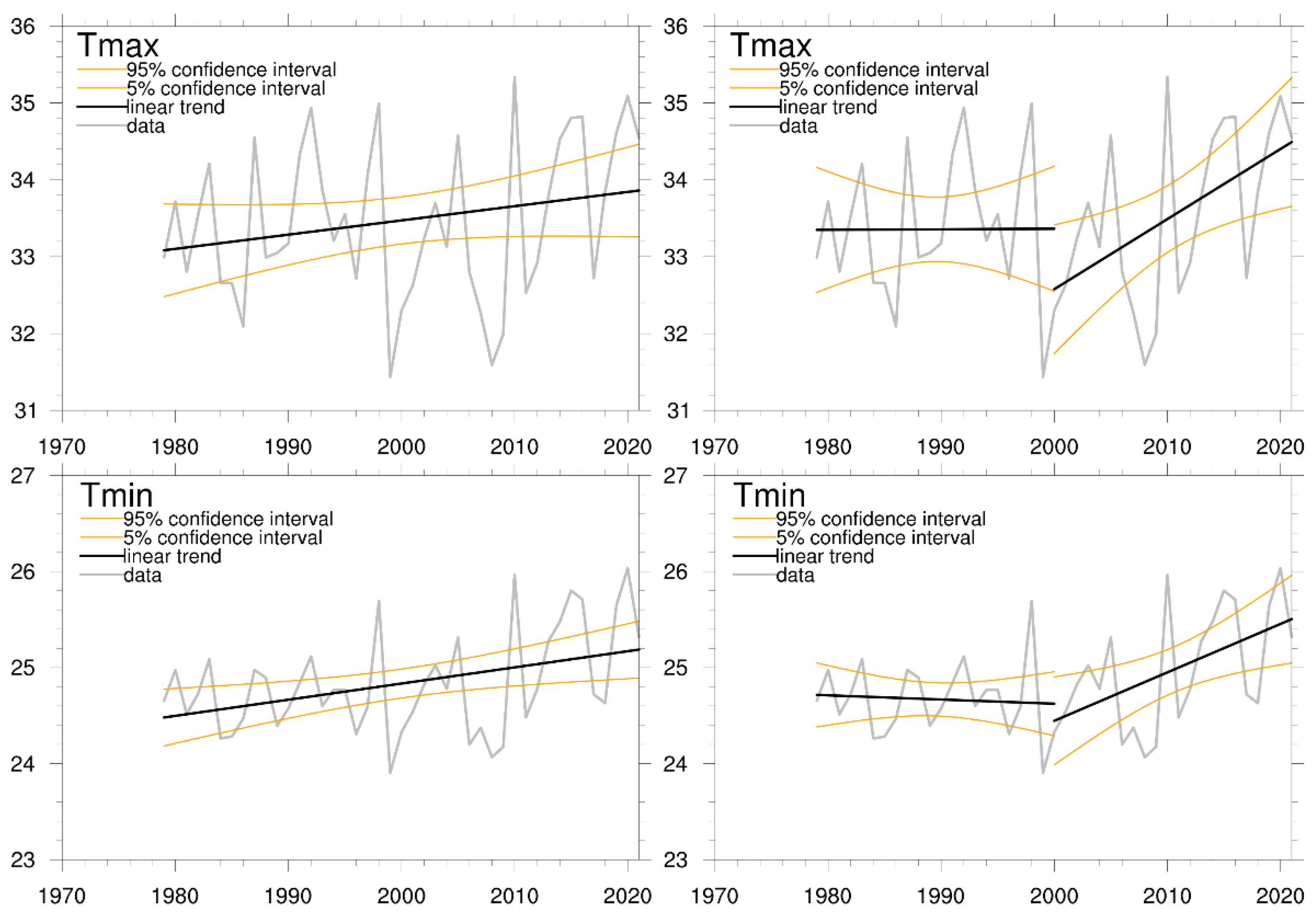
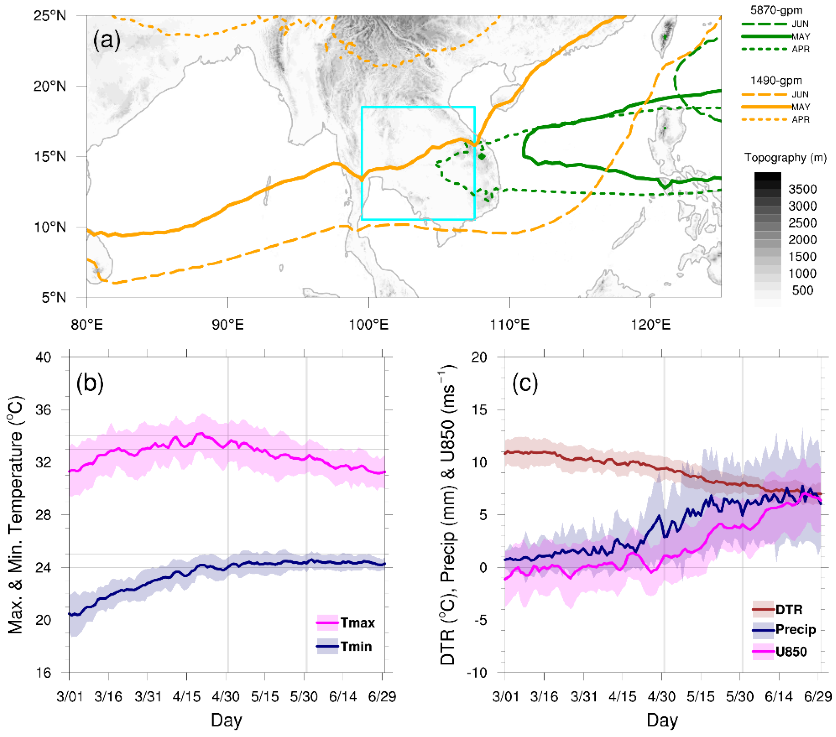
(a) The climatological 5870-gpm (green) and 1490-gpm (orange) contours derived from the 500 and 850 hPa geopotential height fields, respectively, for April, May, and June. The topography is shown in meters. The cyan box denotes the ICP region used in this study. The climatological time series of the area-averaged (b) daily maximum and minimum surface air temperatures (Tmax and Tmin) and (c) diurnal temperature range (DTR), precipitation (Precip), and zonal wind component at 850 hPa (U850) over the ICP region. The solid lines represent the means of daily climatology, while the shaded envelopes enclose the interannual spreads denoted by their respective ± one standard deviation from the mean. The monthly (daily) climatology is computed as a time mean for each calendar month (day) during the period 1979 to 2021. The daily standard deviation is estimated for each calendar day from this 43-year period. The horizontal gray lines in panel (b) indicate 24, 25, 33, and 34 °C. The vertical gray lines indicate 1 May and 31 May, respectively.
Figure 1.
(a) The climatological 5870-gpm (green) and 1490-gpm (orange) contours derived from the 500 and 850 hPa geopotential height fields, respectively, for April, May, and June. The topography is shown in meters. The cyan box denotes the ICP region used in this study. The climatological time series of the area-averaged (b) daily maximum and minimum surface air temperatures (Tmax and Tmin) and (c) diurnal temperature range (DTR), precipitation (Precip), and zonal wind component at 850 hPa (U850) over the ICP region. The solid lines represent the means of daily climatology, while the shaded envelopes enclose the interannual spreads denoted by their respective ± one standard deviation from the mean. The monthly (daily) climatology is computed as a time mean for each calendar month (day) during the period 1979 to 2021. The daily standard deviation is estimated for each calendar day from this 43-year period. The horizontal gray lines in panel (b) indicate 24, 25, 33, and 34 °C. The vertical gray lines indicate 1 May and 31 May, respectively.
![Remotesensing 14 04077 g001]()
Figure 2.
The temporal variations of daily (
a) maximum and (
b) minimum surface temperatures averaged over the ICP region, as shown in
Figure 1a. The vertical axis is the 43-year period from 1979 to 2021, and the horizontal axis is the 90-day span of calendar days from 17 March to 14 June, with the color representing the temperature value for a day of the year. The green color indicates a missing record. Vertical gray lines indicate 1 May and 31 May, respectively.
Figure 3.
(
a) Time series of the standardized monthly anomalies of daily maximum temperature (Tmax), precipitation (Precip), zonal wind component at 850 hPa (U850), and cloud fraction (CF). The analysis period is from 1979 to 2021 for all the variables except CF, for which a shorter period from 2003 to 2021 is applicable. The bar chart displays the winter ONI with pink (light blue) denoting a positive (negative) anomaly. The ONI is the SST anomaly in °C. The blue (red) filled rectangles along the time axis denote the cold (warm) years of a standardized Tmax anomalous value below 0.5 (exceed 1) standard deviation. See text for details. The daily time series of cold (blue) and warm (red) years consist of (
b) daily maximum and minimum temperatures, (
c) diurnal temperature range (DTR) and U850, (
d) precipitation, and (
e) CF. The composites are computed for the 91-day span of calendar days from 1 April to 30 June derived from 8 cold and 8 warm years, respectively, as indicated in panel (
a). Only the cold and warm years during the period from 2003 to 2021 are used for the composites. The horizontal gray lines in panel (
b) indicate 24, 25, 33, and 34 °C. The vertical gray lines indicate 1 May and 31 May, respectively. All the time series shown are area averages over the ICP region, as indicated in
Figure 2a.
![Remotesensing 14 04077 g003]()
Figure 4.
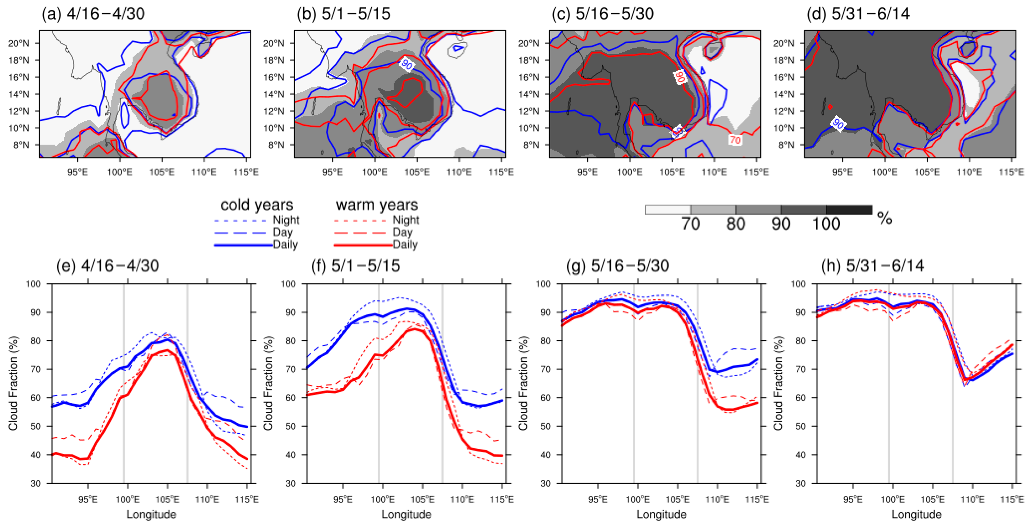
The seasonal variation of cloud fraction (CF) as revealed by averages of four 15-day periods from 16 April to 14 June. (a–d) The spatial distribution of climatological CF (shaded) and composited CF for warm years (red contour) and cold years (blue contour). The CF is a dimensionless quantity and is expressed as a percentage here. The contour interval is 10%; with the first contour at 70%. The plots were derived from daily CF. (e–h) The longitudinal distribution is of composited CF for warm years (red lines) and cold years (blue lines). The daily, daytime, and nighttime CFs are shown. The longitudinal values were obtained by averages from 10.5°N to 18.5°N. The vertical gray lines indicate the western and eastern bounds of the ICP. From left to right panels, the 15-day periods are 16 April to 30 April, 1 May to 15 May, 15 May to 30 May, and 31 May to 14 June, respectively.
Figure 4.
The seasonal variation of cloud fraction (CF) as revealed by averages of four 15-day periods from 16 April to 14 June. (a–d) The spatial distribution of climatological CF (shaded) and composited CF for warm years (red contour) and cold years (blue contour). The CF is a dimensionless quantity and is expressed as a percentage here. The contour interval is 10%; with the first contour at 70%. The plots were derived from daily CF. (e–h) The longitudinal distribution is of composited CF for warm years (red lines) and cold years (blue lines). The daily, daytime, and nighttime CFs are shown. The longitudinal values were obtained by averages from 10.5°N to 18.5°N. The vertical gray lines indicate the western and eastern bounds of the ICP. From left to right panels, the 15-day periods are 16 April to 30 April, 1 May to 15 May, 15 May to 30 May, and 31 May to 14 June, respectively.
Figure 5.
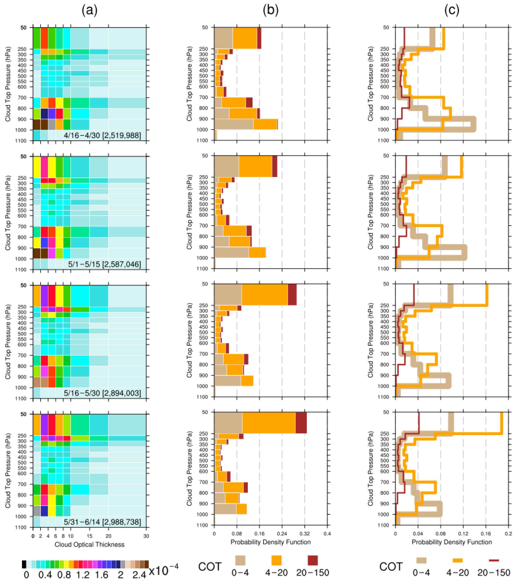
The seasonal variation of the joint probability distribution of the COT binned against CTP for liquid water clouds over the ICP. The seasonal variation is revealed by the statistics of four 15-day periods from 16 April to 14 June in the years from 2003 to 2021. From top to bottom panels, the 15-day periods are 16 April to 30 April, 1 May to 15 May, 15 May to 30 May, and 31 May to 14 June, respectively. (a) The normalized joint probability is displayed as two-dimensional histograms, with COT as the x-axis and CTP as the y-axis. The number in square brackets is the total count for each statistical period. For every bin box, the joint probability value is equal to the bin count divided by the total count (relative frequency). The normalized joint probability in each bin box is computed by dividing the corresponding joint probability value by the bin size (the area of that particular bin box), thereby obtaining the probability density value of the bin box. This normalization is intended to take into account the bin sizes so as to eliminate any visual distortions when comparing bins of different sizes in the two-dimensional histogram plot. The probability of any pixel that falls in a joint histogram bin box can be retrieved after multiplying the corresponding probability density value by that bin size. The bin colors represent the probability density values in each bin. The COT histogram bins ranging from 30 to 150 were chopped off for plotting purposes, owing to the large bin range and very low probability density. The marginal probabilities of CTP with respect to three COT categories are displayed as (b) stacked and (c) overlapping histograms, with probability as the x-axis and CTP as the y-axis. The marginal probabilities of CTP are derived from the joint histograms of COT binned against CTP. The COT is grouped into three categories of newly aggregated bins from the original COT histogram bins: 0–4, 4–20, 20–150. Three sets of the marginal probability of CTP are obtained by integrating (summing) the joint probability over the specific ranges of the aggregated bins from the three COT categories, respectively.
Figure 5.
The seasonal variation of the joint probability distribution of the COT binned against CTP for liquid water clouds over the ICP. The seasonal variation is revealed by the statistics of four 15-day periods from 16 April to 14 June in the years from 2003 to 2021. From top to bottom panels, the 15-day periods are 16 April to 30 April, 1 May to 15 May, 15 May to 30 May, and 31 May to 14 June, respectively. (a) The normalized joint probability is displayed as two-dimensional histograms, with COT as the x-axis and CTP as the y-axis. The number in square brackets is the total count for each statistical period. For every bin box, the joint probability value is equal to the bin count divided by the total count (relative frequency). The normalized joint probability in each bin box is computed by dividing the corresponding joint probability value by the bin size (the area of that particular bin box), thereby obtaining the probability density value of the bin box. This normalization is intended to take into account the bin sizes so as to eliminate any visual distortions when comparing bins of different sizes in the two-dimensional histogram plot. The probability of any pixel that falls in a joint histogram bin box can be retrieved after multiplying the corresponding probability density value by that bin size. The bin colors represent the probability density values in each bin. The COT histogram bins ranging from 30 to 150 were chopped off for plotting purposes, owing to the large bin range and very low probability density. The marginal probabilities of CTP with respect to three COT categories are displayed as (b) stacked and (c) overlapping histograms, with probability as the x-axis and CTP as the y-axis. The marginal probabilities of CTP are derived from the joint histograms of COT binned against CTP. The COT is grouped into three categories of newly aggregated bins from the original COT histogram bins: 0–4, 4–20, 20–150. Three sets of the marginal probability of CTP are obtained by integrating (summing) the joint probability over the specific ranges of the aggregated bins from the three COT categories, respectively.
![Remotesensing 14 04077 g005]()
Figure 6.
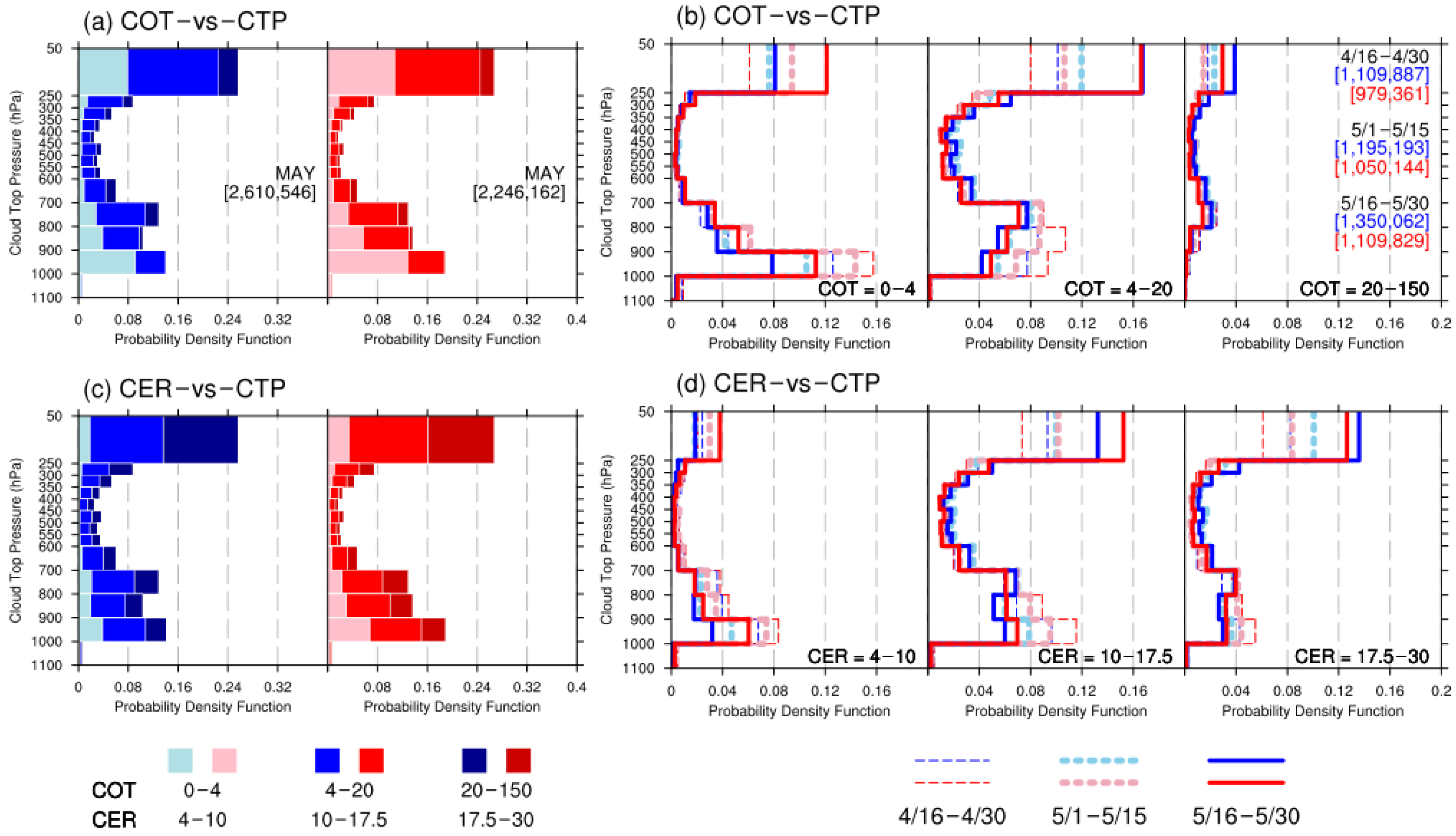
The monthly (May) and seasonal variation of the marginal probabilities of CTP with respect to three categories of (a,b) COT and (c,d) CER, respectively, compiled over the ICP as collected from cold (blue tone) and warm (red tone) years. The seasonal variation is revealed by the statistics of three 15-day periods from 16 April to 30 May of the cold and warm years. The numbers in square brackets are the total counts for these statistical periods; the total counts of CER are equal to COT. The COT and CER are for liquid water clouds in the daytime; COT is a dimensionless quantity, and CER is in μm. The marginal probabilities of CTP are derived from the joint histograms of COT or CER binned against CTP. The COT is grouped into three categories of newly aggregated bins from the original COT histogram bins: 0–4, 4–20, and 20–150, whereas the CER are grouped into three categories of newly aggregated bins from the original CER histogram bins: 4–10,10–17.5, and 17.5–30. Three sets of the marginal probabilities of CTP are obtained by integrating the joint probability (relative frequency) over the specific ranges of the aggregated bins from the three corresponding COT or CER categories, respectively. (a,c) The marginal probabilities of May displayed as stacked histograms. (b,d) The marginal probabilities of 15-day periods displayed as overlapping histograms, with each plot panel for each individual category. The x-axis is probability, the y-axis is CTP.
Figure 6.
The monthly (May) and seasonal variation of the marginal probabilities of CTP with respect to three categories of (a,b) COT and (c,d) CER, respectively, compiled over the ICP as collected from cold (blue tone) and warm (red tone) years. The seasonal variation is revealed by the statistics of three 15-day periods from 16 April to 30 May of the cold and warm years. The numbers in square brackets are the total counts for these statistical periods; the total counts of CER are equal to COT. The COT and CER are for liquid water clouds in the daytime; COT is a dimensionless quantity, and CER is in μm. The marginal probabilities of CTP are derived from the joint histograms of COT or CER binned against CTP. The COT is grouped into three categories of newly aggregated bins from the original COT histogram bins: 0–4, 4–20, and 20–150, whereas the CER are grouped into three categories of newly aggregated bins from the original CER histogram bins: 4–10,10–17.5, and 17.5–30. Three sets of the marginal probabilities of CTP are obtained by integrating the joint probability (relative frequency) over the specific ranges of the aggregated bins from the three corresponding COT or CER categories, respectively. (a,c) The marginal probabilities of May displayed as stacked histograms. (b,d) The marginal probabilities of 15-day periods displayed as overlapping histograms, with each plot panel for each individual category. The x-axis is probability, the y-axis is CTP.
![Remotesensing 14 04077 g006]()
Figure 7.
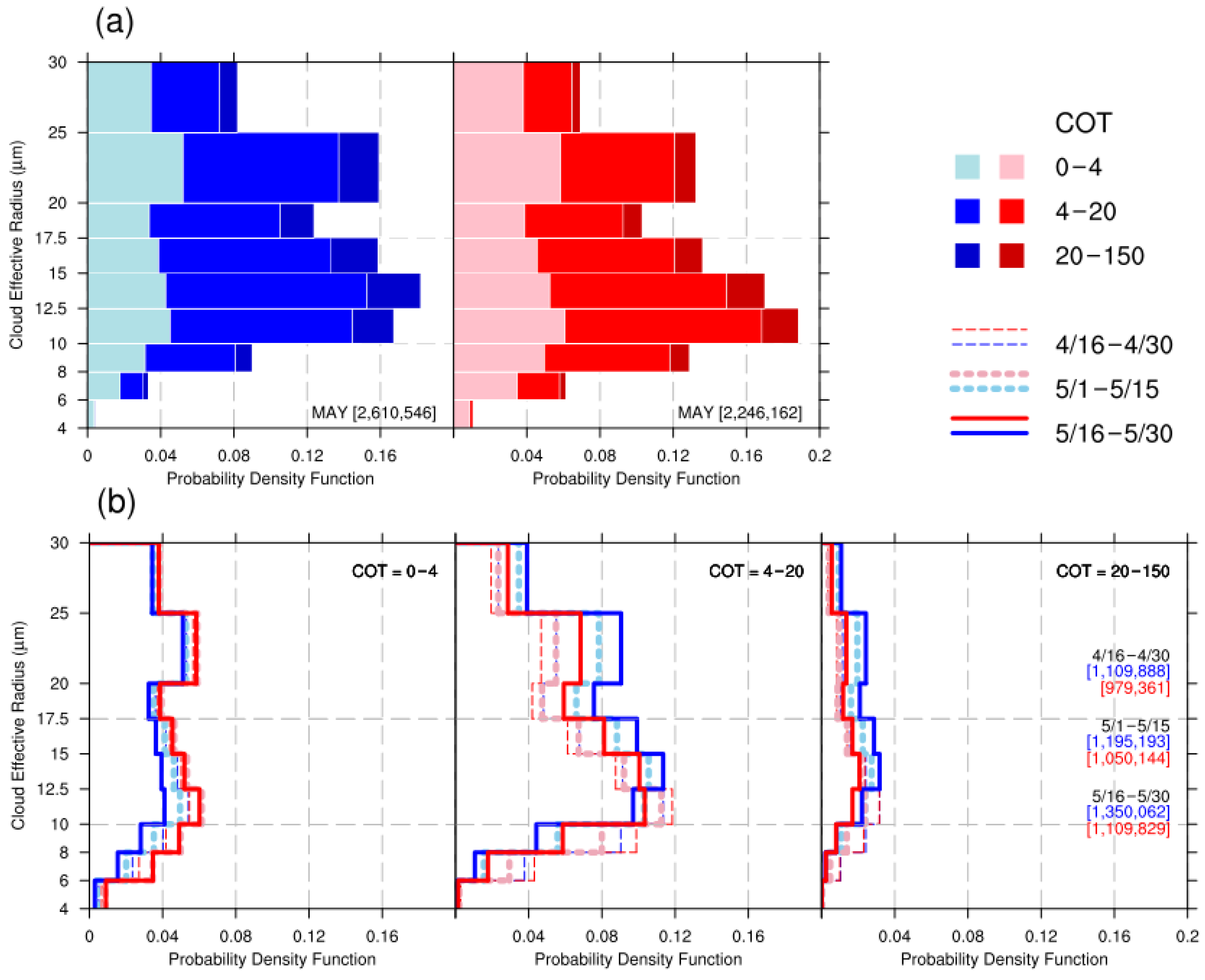
The monthly (May) and seasonal variation of the marginal probabilities of CER with respect to the three categories of COT compiled over the ICP as collected from cold (blue tone) and warm (red tone) years. The seasonal variation is revealed by the statistics of three 15-day periods from 16 April to 30 May of the cold and warm years. The numbers in square brackets are the total counts for these statistical periods. The COT and CER are for liquid water clouds in the daytime; COT is a dimensionless quantity, and CER is in μm. The marginal probabilities of CER are derived from the joint histograms of COT binned against CER. The COT is grouped into three categories of newly aggregated bins from the original COT histogram bins: 0–4, 4–20, and 20–150. Three sets of the marginal probabilities of CER are obtained by integrating the joint probability (relative frequency) over the specific ranges of the aggregated bins from the three corresponding COT categories, respectively. (a) The marginal probabilities of May displayed as stacked histograms. (b) The marginal probabilities of 15-day periods displayed as overlapping histograms, with each plot panel for each individual category. The x-axis is probability, the y-axis is CER.
Figure 7.
The monthly (May) and seasonal variation of the marginal probabilities of CER with respect to the three categories of COT compiled over the ICP as collected from cold (blue tone) and warm (red tone) years. The seasonal variation is revealed by the statistics of three 15-day periods from 16 April to 30 May of the cold and warm years. The numbers in square brackets are the total counts for these statistical periods. The COT and CER are for liquid water clouds in the daytime; COT is a dimensionless quantity, and CER is in μm. The marginal probabilities of CER are derived from the joint histograms of COT binned against CER. The COT is grouped into three categories of newly aggregated bins from the original COT histogram bins: 0–4, 4–20, and 20–150. Three sets of the marginal probabilities of CER are obtained by integrating the joint probability (relative frequency) over the specific ranges of the aggregated bins from the three corresponding COT categories, respectively. (a) The marginal probabilities of May displayed as stacked histograms. (b) The marginal probabilities of 15-day periods displayed as overlapping histograms, with each plot panel for each individual category. The x-axis is probability, the y-axis is CER.
![Remotesensing 14 04077 g007]()
Figure 8.
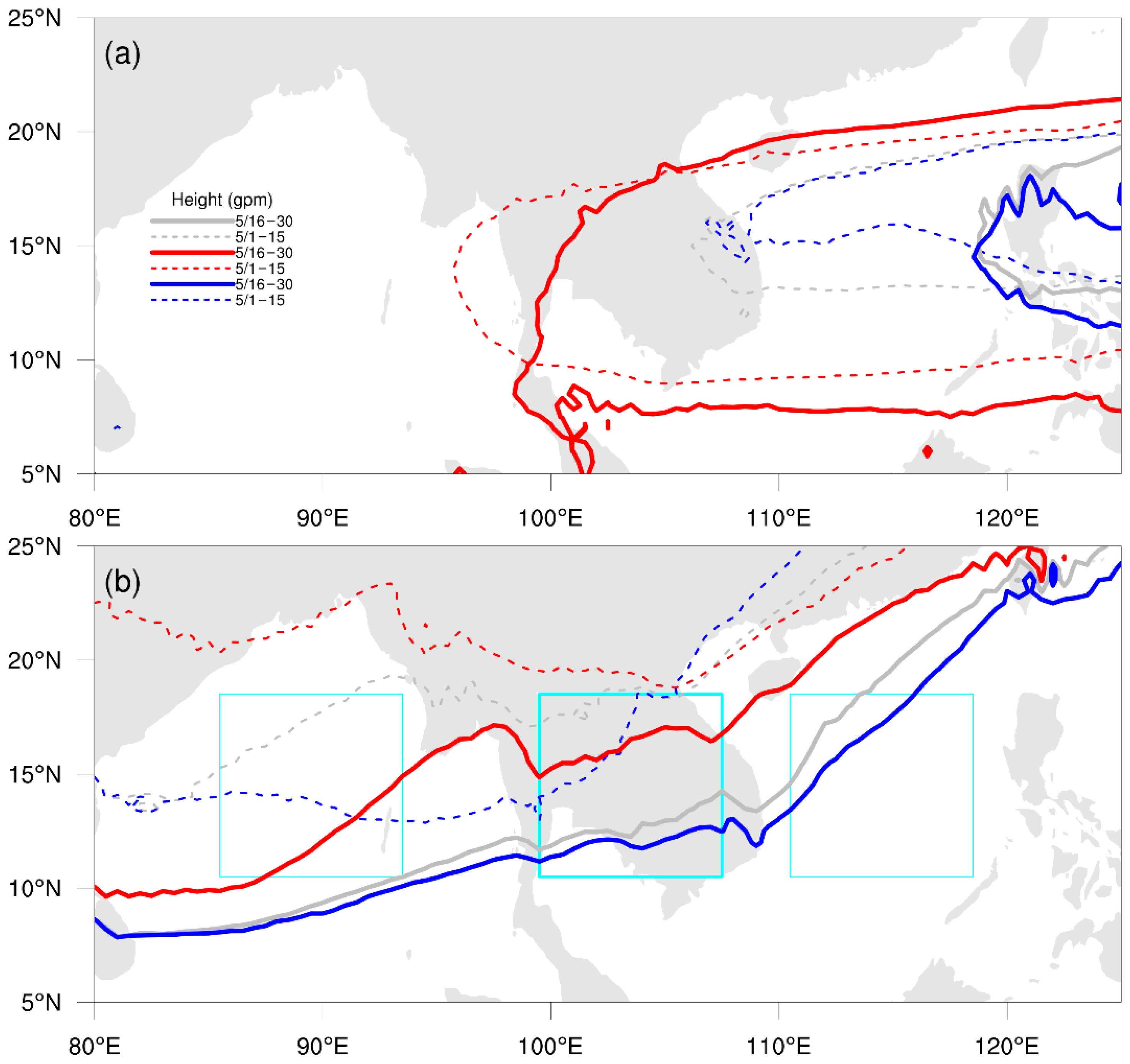
(a) The 5870-gpm (gray and blue) and 5880-gpm (red) contours derived from the composites of 500 hPa geopotential height for climatology, cold, and warm years, respectively. The 5870-gpm is shown for cold years because all the gridded values in the corresponding 500 hPa geopotential height composites over the plotting domain are below 5875-gpm. (b) The 1490-gpm contours derived from the composites of 850 hPa geopotential height for climatology (gray), cold (blue), and warm (red) years. All the composites were computed for the first (solid) and second (dashed) 15-day period of May for climatology (1979–2021), cold, and warm years. The cyan boxes denote the BoB, ICP, and SCS regions with the same area size.
Figure 8.
(a) The 5870-gpm (gray and blue) and 5880-gpm (red) contours derived from the composites of 500 hPa geopotential height for climatology, cold, and warm years, respectively. The 5870-gpm is shown for cold years because all the gridded values in the corresponding 500 hPa geopotential height composites over the plotting domain are below 5875-gpm. (b) The 1490-gpm contours derived from the composites of 850 hPa geopotential height for climatology (gray), cold (blue), and warm (red) years. All the composites were computed for the first (solid) and second (dashed) 15-day period of May for climatology (1979–2021), cold, and warm years. The cyan boxes denote the BoB, ICP, and SCS regions with the same area size.
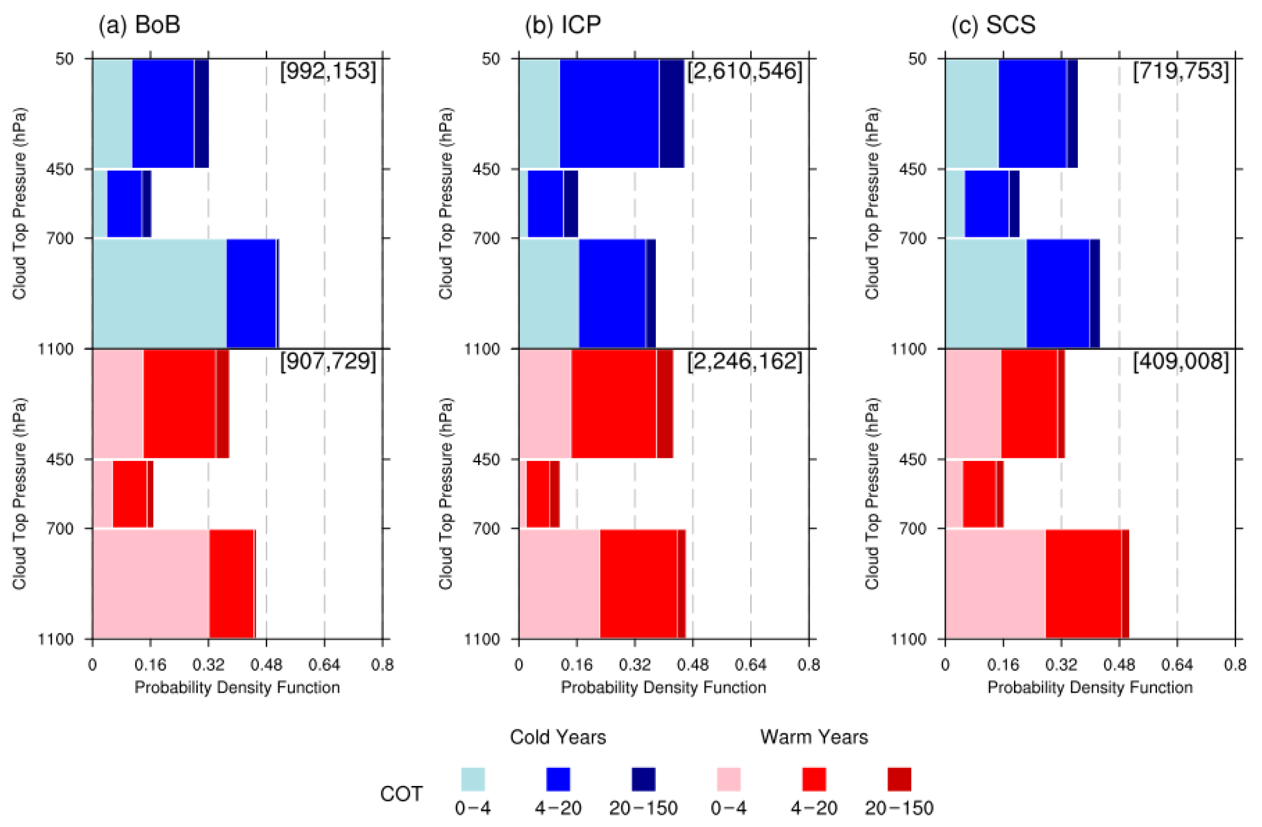
Figure 9.
The marginal probabilities of CTP with respect to three categories of COT compiled over the (
a) BoB, (
b) ICP, and (
c) SCS regions, collected from May of cold (blue tone) and warm (red tone) years. The BoB, ICP, and SCS regions are indicated in
Figure 8b. The COT is for liquid water cloud in the daytime and is a dimensionless quantity, CTP is in hPa. The numbers in square brackets are the total counts for these statistical periods. The marginal probabilities of CTP are derived from the joint histograms of COT binned against CTP and are displayed as stacked histograms with probability as the
x-axis and CTP as the
y-axis. The COT is grouped into three categories of newly aggregated bins from the original COT histogram bins: 0–4, 4–20, and 20–150, whereas the CTP are grouped into three categories of newly aggregated bins from the original CTP histogram bins: 50–450, 440–700, and 700–1100 hPa. For each plot panel, three sets of the marginal probabilities of CTP are obtained by integrating the joint probability (relative frequency) over the specific ranges of the aggregated bins from the three corresponding COT categories, respectively.
![Remotesensing 14 04077 g009]()
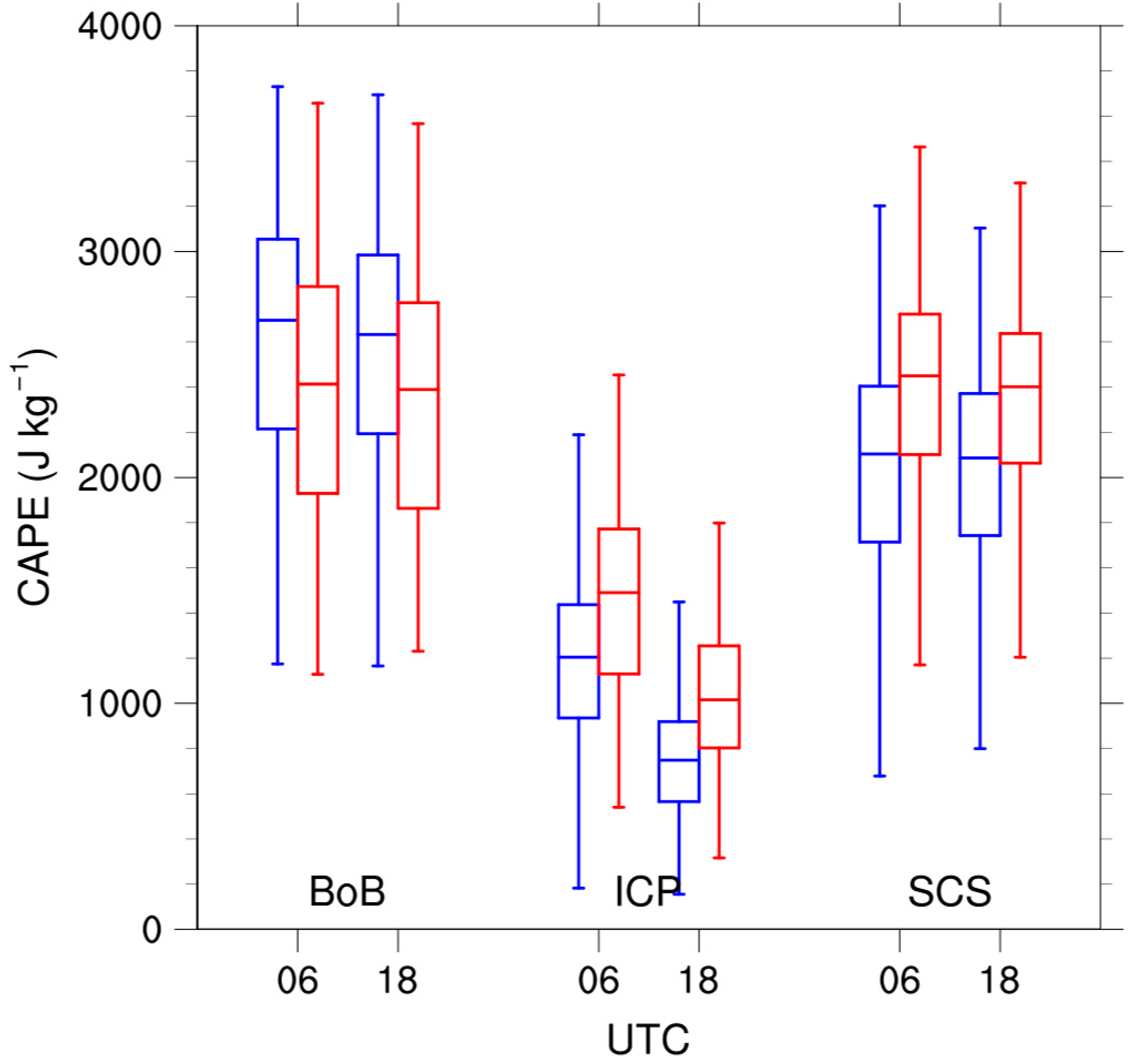
Figure 10.
The box-and-whisker plots for the daily CAPE in May for BoB, ICP, and SCS. The daily CAPE is averaged over the corresponding regions. Blue and red for cold and warm years, respectively. Outliers are excluded by 1.5 interquartile ranges.
Figure 10.
The box-and-whisker plots for the daily CAPE in May for BoB, ICP, and SCS. The daily CAPE is averaged over the corresponding regions. Blue and red for cold and warm years, respectively. Outliers are excluded by 1.5 interquartile ranges.
Figure 11.
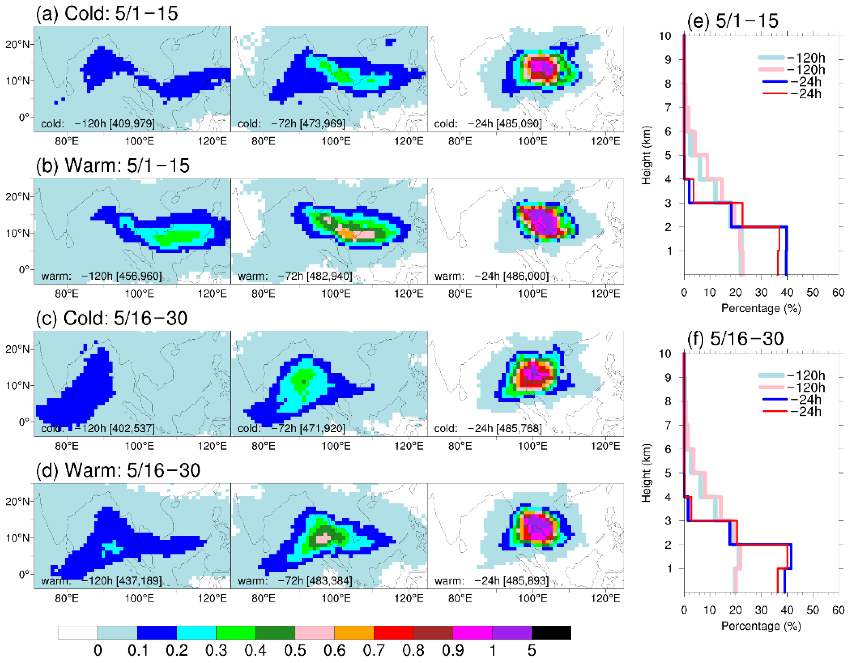
The density distributions of the backward trajectories from the ICP region started within a layer bounded with heights between 1000 and 2000 m above mean sea level. The horizontal distributions of the trajectory density for the 15-day periods of 1–15 May from the (a) cold and (b) warm years and of 16–30 May from the (c) cold and (d) warm years. For each 15-day period, there are 486,000 initial air parcels released and tracked, and their six-hourly horizontal positions are then binned onto a 1° × 1° latitude–longitude grid, from which the histograms are calculated. Using the histograms (count in each grid cell), the trajectory density per grid cell is computed as the percentage of the total. The density of the 120, 72, and 24 h backward trajectories are shown from left to right panels, respectively, in (a–d). The numbers in square brackets are the total counts of the trajectory remaining in the domain at the corresponding backward times. The vertical distributions of the trajectory density were collected in the 15-day periods of (e) 1–15 May and (f) 16–30 May. The six-hourly trajectory histograms of the horizontal positions are further binned with respect to the trajectory altitudes using 1 km increments, and the domain-wide trajectory density per 1 km increment is computed as the percentage of the total. Trajectory densities from warm and cold years are superimposed for comparison.
Figure 11.
The density distributions of the backward trajectories from the ICP region started within a layer bounded with heights between 1000 and 2000 m above mean sea level. The horizontal distributions of the trajectory density for the 15-day periods of 1–15 May from the (a) cold and (b) warm years and of 16–30 May from the (c) cold and (d) warm years. For each 15-day period, there are 486,000 initial air parcels released and tracked, and their six-hourly horizontal positions are then binned onto a 1° × 1° latitude–longitude grid, from which the histograms are calculated. Using the histograms (count in each grid cell), the trajectory density per grid cell is computed as the percentage of the total. The density of the 120, 72, and 24 h backward trajectories are shown from left to right panels, respectively, in (a–d). The numbers in square brackets are the total counts of the trajectory remaining in the domain at the corresponding backward times. The vertical distributions of the trajectory density were collected in the 15-day periods of (e) 1–15 May and (f) 16–30 May. The six-hourly trajectory histograms of the horizontal positions are further binned with respect to the trajectory altitudes using 1 km increments, and the domain-wide trajectory density per 1 km increment is computed as the percentage of the total. Trajectory densities from warm and cold years are superimposed for comparison.
![Remotesensing 14 04077 g011]()
Figure 12.
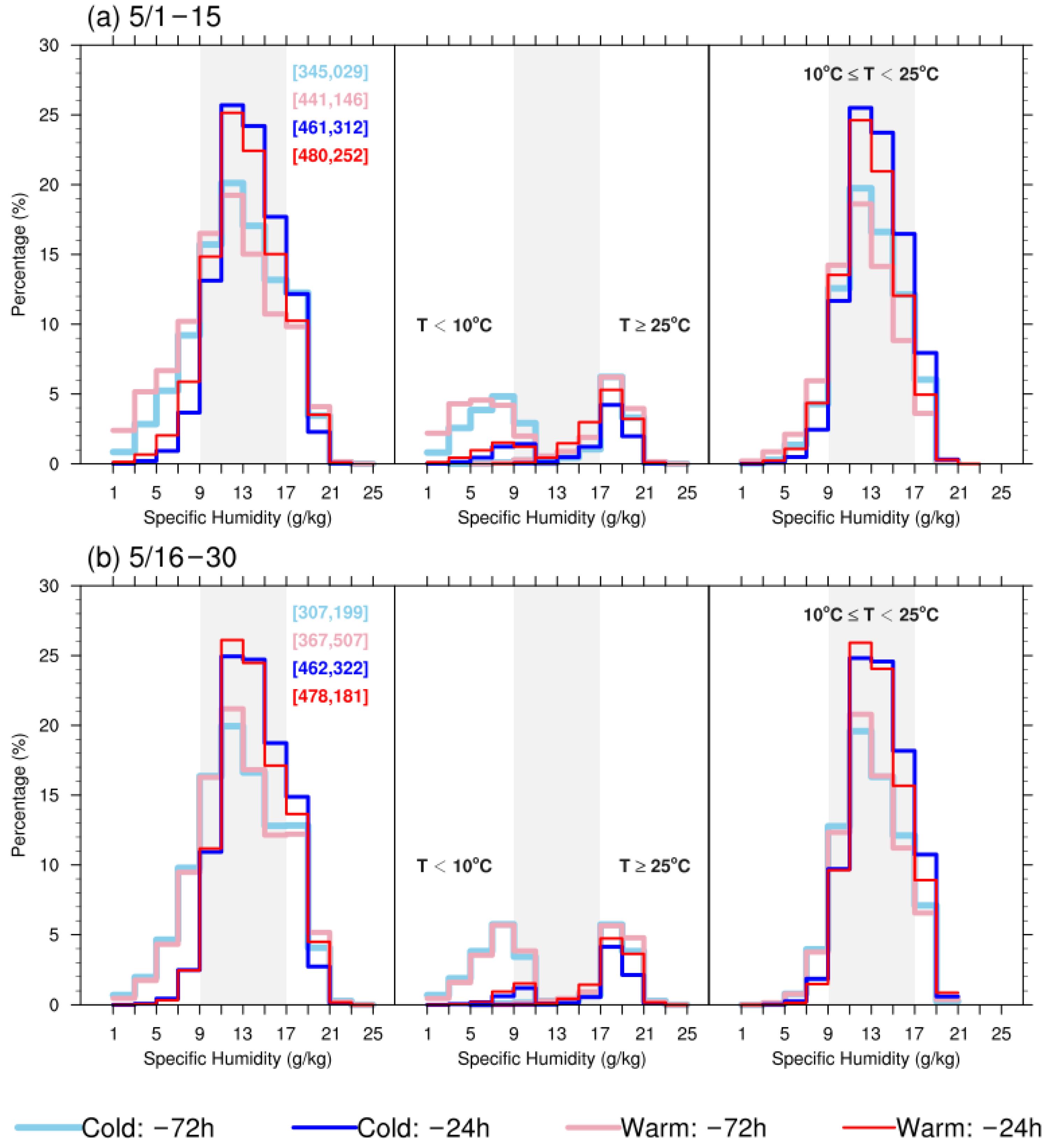
The probability distributions of the specific humidity carried by the backward trajectories at the backward times of 72 and 24 h are presented for the 15-day periods of (a) 1–15 May and (b) 16–30 May. The probability is computed as a relative frequency; that is, the counts in each humidity bin divided by the total counts of the trajectory remaining within a subdomain (5°–18°N, 80°–120°E) at the corresponding backward times. Similar patterns of distributions are obtained by using the calculation domain (10°S–25°N, 70°–130°E) for backward trajectory. The left panels are for the specific humidity from all trajectories; the central and right panels are the marginal probability of specific humidity with respect to the temperature values. The numbers in square brackets (left panels) are the total counts of the trajectory remaining in the subdomain at the corresponding backward times.
Figure 12.
The probability distributions of the specific humidity carried by the backward trajectories at the backward times of 72 and 24 h are presented for the 15-day periods of (a) 1–15 May and (b) 16–30 May. The probability is computed as a relative frequency; that is, the counts in each humidity bin divided by the total counts of the trajectory remaining within a subdomain (5°–18°N, 80°–120°E) at the corresponding backward times. Similar patterns of distributions are obtained by using the calculation domain (10°S–25°N, 70°–130°E) for backward trajectory. The left panels are for the specific humidity from all trajectories; the central and right panels are the marginal probability of specific humidity with respect to the temperature values. The numbers in square brackets (left panels) are the total counts of the trajectory remaining in the subdomain at the corresponding backward times.
Table 1.
The ICP cold and warm years and the corresponding seasonal ENSO conditions as revealed by the preceding winter and spring ONI. The cold, warm, and neutral conditions are denoted as characters C, W, and N, respectively, in the square brackets. The first (second) character is for winter (spring) ONI. Note that only seven cold years can be identified after the year 2003; the year 2004, with an anomalous value of −0.34, was selected to be a cold year to ensure the same sample size for the warm-year and cold-year composites.
| | ENSO-Related | Non-ENSO Factors |
|---|
| Cold years | 2006 [CC], 2008 [CC], 2009 [CC],
2011 [CC], 2012 [CC] | 2004 [NN], 2017 [NN]
2007 [WN] |
| Warm years | 2005 [WN], 2010 [WW], 2015 [WW],
2016 [WW], 2019 [WW] | 2014 [NN], 2020 [NN]
2021 [CC] |
Table 2.
The correlation coefficients between the preceding winter (spring) ONI and some monthly atmospheric variables over the ICP region of May for three different periods: 1979–2000, 2000–2021, and 1979–2021. The correlation coefficients calculated against spring ONI are given in parentheses. Correlation coefficient values that exceed 0.424 (df = 20) and 0.3 (df = 41) are statistically significant at the 95% level (p < 0.05). The bold numbers indicate that the differences between the correlation coefficients for 1979–2000 and 2000–2021 are statistically significant at the 95% level (p < 0.05).
| | Tmax | Tmin | H500 | H850 | U850 | Precip | CF |
|---|
| 1979–2000 | 0.80 (0.87) | 0.92 (0.89) | 0.68 (0.63) | 0.58 (0.61) | −0.07 (−0.06) | −0.41 (−0.52) | |
| 2000–2021 | 0.66 (0.69) | 0.69 (0.73) | 0.65 (0.70) | 0.40 (0.45) | −0.04 (−0.05) | −0.41 (−0.41) | −0.40 (−0.38) |
| 1979–2021 | 0.69 (0.73) | 0.68 (0.67) | 0.50 (0.47) | 0.45 (0.48) | −0.02 (−0.02) | −0.37 (−0.42) | |


