
Integration Data Model of the Bathymetric Monitoring System for Shallow Waterbodies Using UAV and USV Platforms †

 ,
,  ,
,  ,
,  ,
,  ,
,  ,
,
Abstract
1. Introduction
2. Materials and Methods
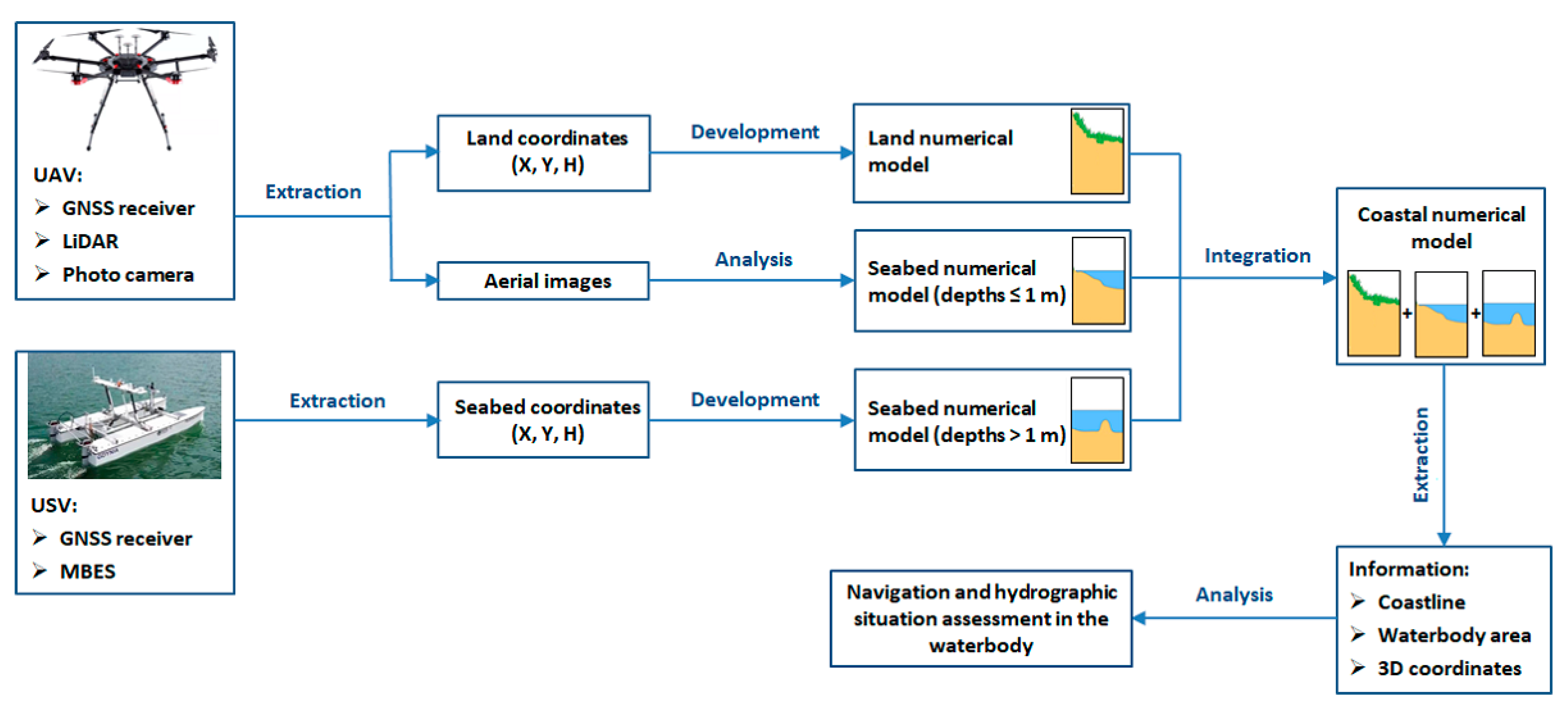
2.1. Hydroacoustic and Optoelectronic Data Integration Component
- Direction angles (δ) (°);
- Averaged rotation angle (θ) (°);
- Three elementary rotation matrices around the axes OX, OY and OZ of the 3D coordinate system (Rx, Ry, Rz) (–);
- Scale factor (S) (–);
- Three-dimensional coordinates of the translation vector () (–).
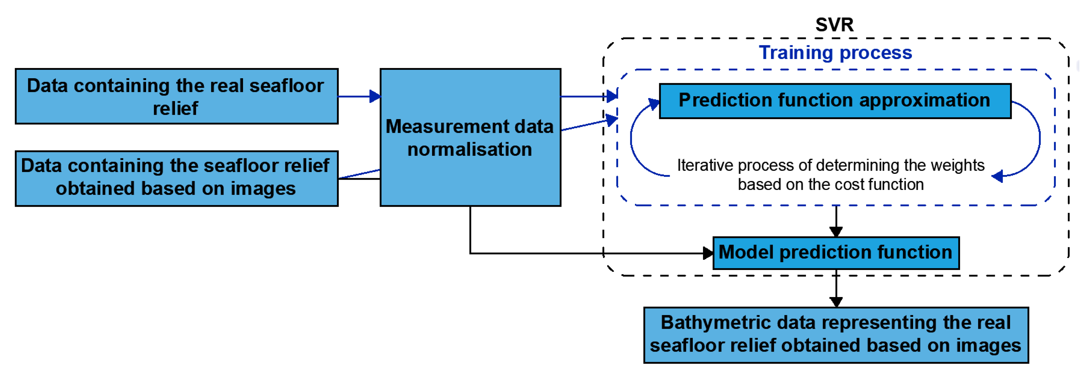
2.2. Radiometric Depth Determination Component Based on Optoelectronic Data
2.3. Coastline Extraction Component
- The method must only be used for the coastline extraction from a DTM or a point cloud;
- Measurement data will be obtained only by Airborne Laser Scanning (ALS). This means the rejection of methods based on multisensory fusion, even if the fusion involves ALS;
- Due to the rapid development of geoinformatics and computational techniques, the proposed method had to be published within the last 10 years (2011–2021).
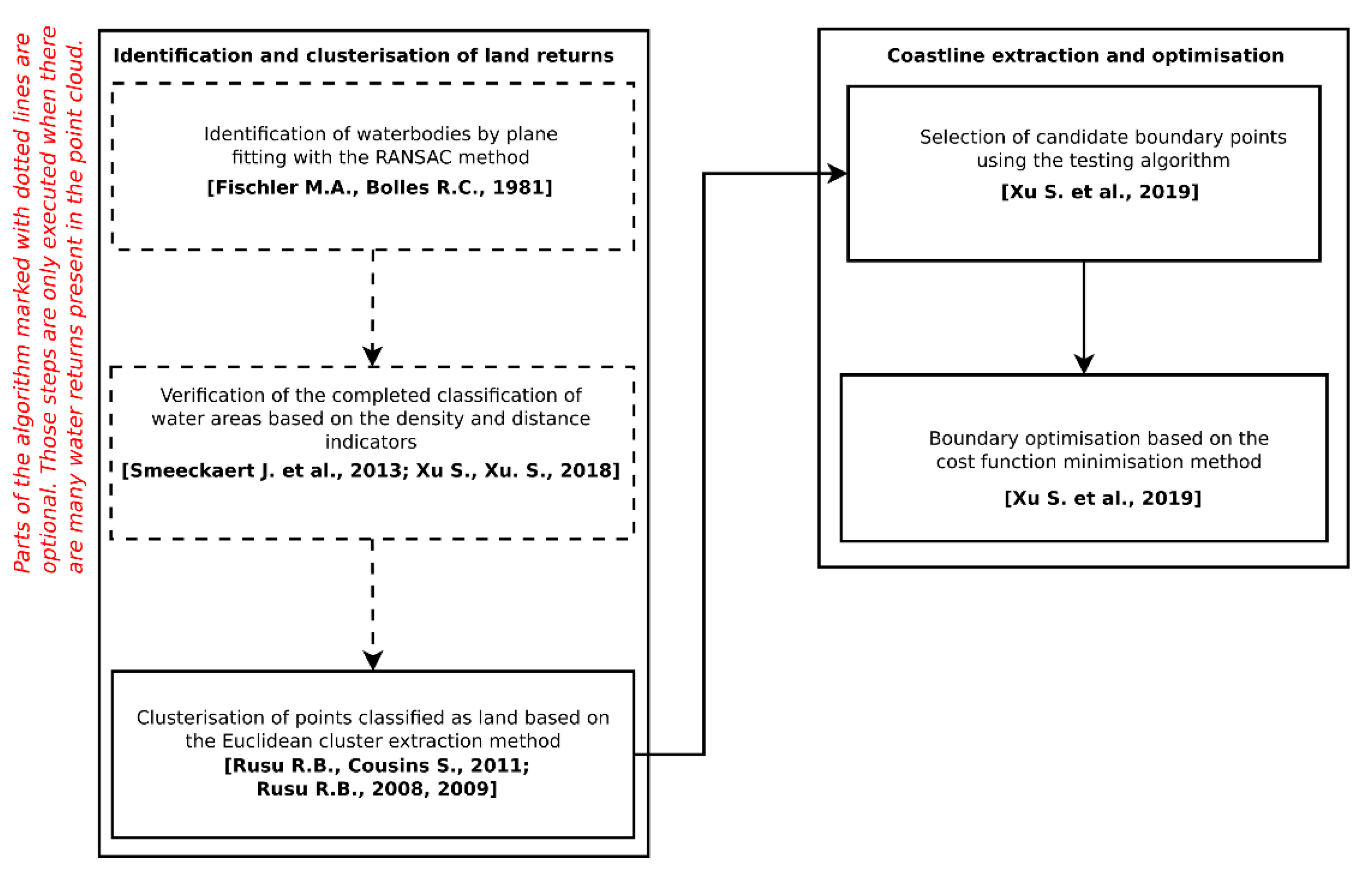
- This step is only performed if the user marks the original LiDAR point cloud, which contains many water returns. Classification of particular clusters as water or land clusters based on the assumption of water area flatness. To this end, plane fitting by the RANSAC method is used [97]. Successive steps of the RANSAC algorithm when solving the plane fitting problem can be described as follows [95]:
- Randomly select three non-collinear points p from the set of points P;
- Based on the selected points, calculate the coefficients of the plane model equation;
- Calculate the distance between the plane model and each point p;
- Calculate the number of points p whose distance from the plane is smaller than the threshold value Є provided by the user.
The RANSAC algorithm is iterative in nature. Its performance is repeated for a max of N times until the percentage of the points located within the tolerance limits Є is no greater than τ [98]. According to the authors [87], the above approach allows for identification of waterbodies larger than 500 m × 500 m. - This step is only performed if the user marks the original LiDAR point cloud, which contains many water returns. Verification of the completed classification of water areas based on the density and distance indicators [96] calculated for individual points. This is because the reflections from the water surface, identified based on the flatness index, can also originate from flat land areas. At this stage, two characteristics are calculated: point density (D), which is calculated in a rectangular window of the predefined size for every point in the cloud and the elevation of each point in the cloud above its nearest extracted plane (E). The above characteristics allow for reclassification of points. Points are converted to the land class if the point density Dc calculated in the predefined window is greater than the adopted threshold value TD:Moreover, selected points are removed from the LiDAR cloud. A point is removed if its elevation above the nearest plane E is greater than the threshold value Te:
- Clusterisation of points classified as land (or all points in case the previous steps were not performed) based on the Euclidean cluster extraction method [94,95,99]. The rejection of clusters containing fewer than np points. It should be noted that if not too many reflections from water were noted during laser scanning, this stage already enables a significant reduction in water points in the cloud. Otherwise (e.g., in shallow waterbodies), this procedure will not ensure the removal of water points from the cloud [84], hence why authors [87] proposed the two optional steps for the case of abundant water reflections, which were described above.
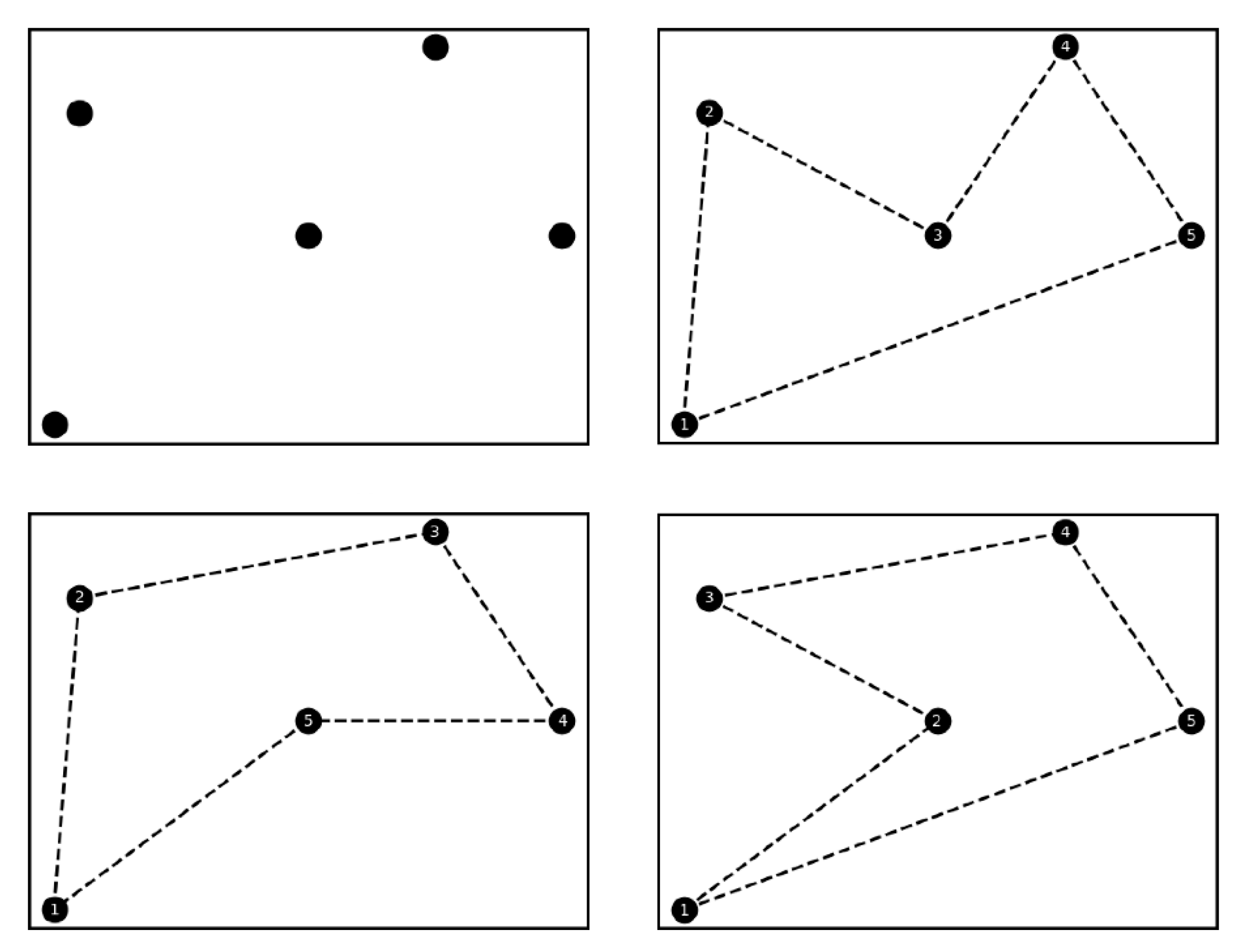
- Selection of candidate boundary points using the test algorithm [87]. During the initialisation, all points are regarded as indeterminate ones. In each step, if point p is an indeterminate point, it is necessary to select its k-nearest neighbours and, based on them, to construct a convex hull. It should be noted that in the convex hull, point p is not a boundary point of the convex set S, if it is located within a triangle whose vertices are located in S [100]. Hence, the points formed within the hull can be regarded as points that do not form the coastline. This process is iteratively repeated until there are no more points that can be eliminated in the above manner. Moreover, if a point is located further than Td from the remaining points, it will be regarded as an error and immediately removed. A problem at this stage of the algorithm operation is the ambiguity of determining the coastline course based on the obtained set of points. For example, for 5 points, it is possible to indicate many different ways to combine them, thus obtaining many different potential coastline courses (Figure 6).
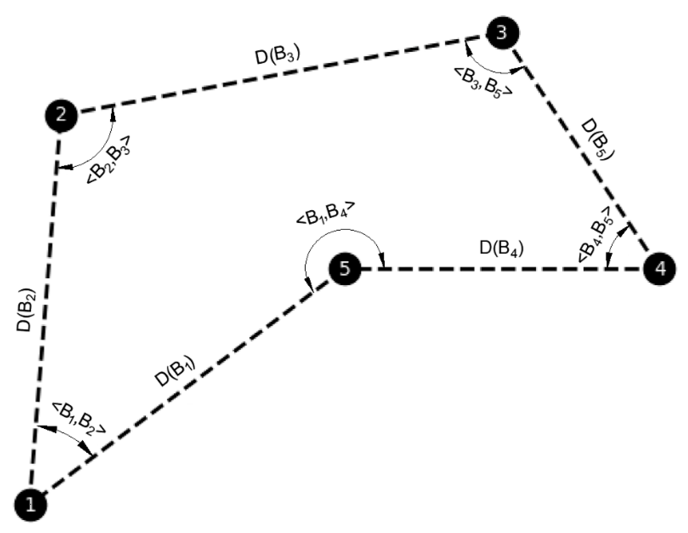
- Boundary optimisation based on the cost function minimisation method [87]. As there are many potential coastline courses, it is necessary to define the criterion for assessing individual connections. It is proposed that the principle of parsimony should be used [101], according to which, if a particular phenomenon or process can be explained in many ways, the one with the lowest cost (the simplest and most economical) will be the most probable. In order to assess the cost of coastline formation, the boundary cost β (m) is defined as follows:where:n—number of connections in the formed boundary (–),D(Bi)—length of the connection Bi (m),λ—weight coefficient (–),N—number of connections in the formed boundary (–),<Bi,Bj>—angle between connections Bi and Bj (°).It should be noted that the minimisation of Equation (15) occurs when the boundary points are located close to each other, and the angles between individual connections are wide (Figure 7).
3. Discussion and Conclusions
Author Contributions
Funding
Data Availability Statement
Conflicts of Interest
References
- Giordano, F.; Mattei, G.; Parente, C.; Peluso, F.; Santamaria, R. Integrating Sensors into a Marine Drone for Bathymetric 3D Surveys in Shallow Waters. Sensors 2016, 16, 41. [Google Scholar] [CrossRef] [PubMed]
- Giordano, F.; Mattei, G.; Parente, C.; Peluso, F.; Santamaria, R. MicroVEGA (Micro Vessel for Geodetics Application): A Marine Drone for the Acquisition of Bathymetric Data for GIS Applications. Int. Arch. Photogramm. Remote Sens. Spat. Inf. Sci. 2015, 40, 123–130. [Google Scholar] [CrossRef]
- Jin, J.; Zhang, J.; Shao, F.; Lyu, Z.; Wang, D. A Novel Ocean Bathymetry Technology Based on an Unmanned Surface Vehicle. Acta Oceanol. Sin. 2018, 37, 99–106. [Google Scholar] [CrossRef]
- Liang, J.; Zhang, J.; Ma, Y.; Zhang, C.-Y. Derivation of Bathymetry from High-resolution Optical Satellite Imagery and USV Sounding Data. Mar. Geod. 2017, 40, 466–479. [Google Scholar] [CrossRef]
- Lubczonek, J.; Kazimierski, W.; Zaniewicz, G.; Lacka, M. Methodology for Combining Data Acquired by Unmanned Surface and Aerial Vehicles to Create Digital Bathymetric Models in Shallow and Ultra-shallow Waters. Remote Sens. 2022, 14, 105. [Google Scholar] [CrossRef]
- Nikolakopoulos, K.G.; Lampropoulou, P.; Fakiris, E.; Sardelianos, D.; Papatheodorou, G. Synergistic Use of UAV and USV Data and Petrographic Analyses for the Investigation of Beachrock Formations: A Case Study from Syros Island, Aegean Sea, Greece. Minerals 2018, 8, 534. [Google Scholar] [CrossRef]
- Specht, M.; Specht, C.; Stateczny, A.; Marchel, Ł.; Lewicka, O.; Paliszewska-Mojsiuk, M.; Wiśniewska, M. Determining the Seasonal Variability of the Territorial Sea Baseline in Poland (2018–2020) Using Integrated USV/GNSS/SBES Measurements. Energies 2021, 14, 2693. [Google Scholar] [CrossRef]
- Specht, M.; Specht, C.; Szafran, M.; Makar, A.; Dąbrowski, P.; Lasota, H.; Cywiński, P. The Use of USV to Develop Navigational and Bathymetric Charts of Yacht Ports on the Example of National Sailing Centre in Gdańsk. Remote Sens. 2020, 12, 2585. [Google Scholar] [CrossRef]
- Stateczny, A.; Grońska, D.; Motyl, W. Hydrodron—New Step for Professional Hydrography for Restricted Waters. In Proceedings of the Baltic Geodetic Congress 2018 (BGC 2018), Olsztyn, Poland, 21–23 June 2018. [Google Scholar]
- Suhari, K.T.; Karim, H.; Gunawan, P.H.; Purwanto, H. Small ROV Marine Boat for Bathymetry Surveys of Shallow Waters—Potential Implementation in Malaysia. Int. Arch. Photogramm. Remote Sens. Spat. Inf. Sci.-ISPRS Arch. 2017, XLII-4/W5, 201–208. [Google Scholar] [CrossRef]
- Alevizos, E.; Oikonomou, D.; Argyriou, A.V.; Alexakis, D.D. Fusion of Drone-based RGB and Multi-spectral Imagery for Shallow Water Bathymetry Inversion. Remote Sens. 2022, 14, 1127. [Google Scholar] [CrossRef]
- Bagheri, O.; Ghodsian, M.; Saadatseresht, M. Reach Scale Application of UAV+SfM Method in Shallow Rivers Hyperspatial Bathymetry. Int. Arch. Photogramm. Remote Sens. Spat. Inf. Sci. 2015, XL-1/W5, 77–81. [Google Scholar] [CrossRef]
- Bandini, F.; Lopez-Tamayo, A.; Merediz-Alonso, G.; Olesen, D.; Jakobsen, J.; Wang, S.; Garcia, M.; Bauer-Gottwein, P. Unmanned Aerial Vehicle Observations of Water Surface Elevation and Bathymetry in the Cenotes and Lagoons of the Yucatan Peninsula, Mexico. Hydrogeol. J. 2018, 26, 2213–2228. [Google Scholar] [CrossRef]
- Bandini, F.; Olesen, D.; Jakobsen, J.; Kittel, C.M.M.; Wang, S.; Garcia, M.; Bauer-Gottwein, P. Technical Note: Bathymetry Observations of Inland Water Bodies Using a Tethered Single-beam Sonar Controlled by an Unmanned Aerial Vehicle. Hydrol. Earth Syst. Sci. 2018, 22, 4165–4181. [Google Scholar] [CrossRef]
- He, J.; Lin, J.; Ma, M.; Liao, X. Mapping Topo-bathymetry of Transparent Tufa Lakes Using UAV-based Photogrammetry and RGB Imagery. Geomorphology 2021, 389, 107832. [Google Scholar] [CrossRef]
- Kim, J.S.; Baek, D.; Seo, I.W.; Shin, J. Retrieving Shallow Stream Bathymetry from UAV-assisted RGB Imagery Using a Geospatial Regression Method. Geomorphology 2019, 341, 102–114. [Google Scholar] [CrossRef]
- Massuel, S.; Feurer, D.; El Maaoui, M.A.; Calvez, R. Deriving Bathymetries from Unmanned Aerial Vehicles: A Case Study of a Small Intermittent Reservoir. Hydrol. Sci. J. 2022, 67, 82–93. [Google Scholar] [CrossRef]
- Panlilio, K.; Pedido, S.M.; Ramos, R.; Tamondong, A. Bathymetric Mapping of Shallow Waters in Lian, Batangas Using Unmanned Aerial Vehicle (UAV). In Proceedings of the 40th Asian Conference on Remote Sensing (ACRS 2019), Daejeon, Korea, 14–18 October 2019. [Google Scholar]
- Cao, B.; Fang, Y.; Jiang, Z.; Gao, L.; Hu, H. Shallow Water Bathymetry from WorldView-2 Stereo Imagery Using Two-media Photogrammetry. Eur. J. Remote Sens. 2019, 52, 506–521. [Google Scholar] [CrossRef]
- Popielarczyk, D.; Marschalko, M.; Templin, T.; Niemiec, D.; Yilmaz, I.; Matuszková, B. Bathymetric Monitoring of Alluvial River Bottom Changes for Purposes of Stability of Water Power Plant Structure with a New Methodology for River Bottom Hazard Mapping (Wloclawek, Poland). Sensors 2020, 20, 5004. [Google Scholar] [CrossRef]
- Khazaei, B.; Read, L.K.; Casali, M.; Sampson, K.M.; Yates, D.N. GLOBathy, the Global Lakes Bathymetry Dataset. Sci. Data 2022, 9, 36. [Google Scholar] [CrossRef]
- Erena, M.; Atenza, J.F.; García-Galiano, S.; Domínguez, J.A.; Bernabé, J.M. Use of Drones for the Topo-bathymetric Monitoring of the Reservoirs of the Segura River Basin. Water 2019, 11, 445. [Google Scholar] [CrossRef]
- Pratomo, D.G.; Khomsin; Putranto, B.F.E. Analysis of the Green Light Penetration from Airborne LiDAR Bathymetry in Shallow Water Area. In IOP Conference Series: Earth and Environmental Science; IOP Publishing: Bristol, UK, 2019; Volume 389, p. 012003. [Google Scholar]
- Wang, D.; Xing, S.; He, Y.; Yu, J.; Xu, Q.; Li, P. Evaluation of a New Lightweight UAV-borne Topo-bathymetric LiDAR for Shallow Water Bathymetry and Object Detection. Sensors 2022, 22, 1379. [Google Scholar] [CrossRef]
- Hattori, N.; Sato, S.; Yamanaka, Y. Development of an Imagery-based Monitoring System for Nearshore Bathymetry by Using Wave Breaking Density. Coast. Eng. 2019, 61, 308–320. [Google Scholar] [CrossRef]
- Salameh, E.; Frappart, F.; Almar, R.; Baptista, P.; Heygster, G.; Lubac, B.; Raucoules, D.; Almeida, L.P.; Bergsma, E.W.J.; Capo, S.; et al. Monitoring Beach Topography and Nearshore Bathymetry Using Spaceborne Remote Sensing: A Review. Remote Sens. 2019, 11, 2212. [Google Scholar] [CrossRef]
- Specht, M.; Stateczny, A.; Specht, C.; Widźgowski, S.; Lewicka, O.; Wiśniewska, M. Concept of an Innovative Autonomous Unmanned System for Bathymetric Monitoring of Shallow Waterbodies (INNOBAT System). Energies 2021, 14, 5370. [Google Scholar] [CrossRef]
- IHO. IHO Standards for Hydrographic Surveys, 6th ed.; Special Publication No. 44; IHO: Monaco, Monaco, 2020. [Google Scholar]
- Specht, C.; Lewicka, O.; Specht, M.; Dąbrowski, P.; Burdziakowski, P. Methodology for Carrying out Measurements of the Tombolo Geomorphic Landform Using Unmanned Aerial and Surface Vehicles near Sopot Pier, Poland. J. Mar. Sci. Eng. 2020, 8, 384. [Google Scholar] [CrossRef]
- Hogrefe, K.R.; Wright, D.J.; Hochberg, E.J. Derivation and Integration of Shallow-water Bathymetry: Implications for Coastal Terrain Modeling and Subsequent Analyses. Mar. Geod. 2008, 31, 299–317. [Google Scholar] [CrossRef]
- Kulawiak, M.; Chybicki, A. Application of Web-GIS and Geovisual Analytics to Monitoring of Seabed Evolution in South Baltic Sea Coastal Areas. Mar. Geod. 2018, 41, 405–426. [Google Scholar] [CrossRef]
- Warnasuriya, T.W.S.; Gunaalan, K.; Gunasekara, S.S. Google Earth: A New Resource for Shoreline Change Estimation—Case Study from Jaffna Peninsula, Sri Lanka. Mar. Geod. 2018, 41, 546–580. [Google Scholar] [CrossRef]
- Lihua, Z.; Shuaidong, J.; Rencan, P.; Jian, D.; Ning, L. A Quantitative Method to Control and Adjust the Accuracy of Adaptive Grid Depth Modeling. Mar. Geod. 2013, 36, 408–427. [Google Scholar] [CrossRef]
- Makar, A. The Sea Bottom Surface Described by Coons Pieces. Sci. J. Marit. Univ. Szczec. 2016, 45, 187–190. [Google Scholar]
- Sassais, R.; Makar, A. Methods to Generate Numerical Models of Terrain for Spatial ENC Presentation. Annu. Navig. 2011, 18, 1–13. [Google Scholar]
- Aurelia Technologies Inc. Aurelia X8 Standard. Available online: https://aurelia-aerospace.com/product/aurelia-x8-standard/ (accessed on 19 August 2022).
- SBG Systems. Ellipse-D. Available online: https://www.sbg-systems.com/products/ellipse-series/#ellipse-d_rtk_gnss_ins (accessed on 19 August 2022).
- SBG Systems. Ekinox Series. Available online: https://www.sbg-systems.com/products/ekinox-series/ (accessed on 19 August 2022).
- Velodyne Lidar. Puck LITE. Available online: https://velodynelidar.com/products/puck-lite/ (accessed on 19 August 2022).
- Sony Corporation. α6500 Premium E-mount APS-C Camera. Available online: https://www.sony.com/en-ae/electronics/interchangeable-lens-cameras/ilce-6500-body-kit (accessed on 19 August 2022).
- Sony Corporation. E 35mm F1.8 OSS. Available online: https://www.sony.com/en-ae/electronics/camera-lenses/sel35f18 (accessed on 19 August 2022).
- Gremsy. GREMSY T3V3. Available online: https://gremsy.com/gremsy-t3v3-store (accessed on 19 August 2022).
- Burdziakowski, P.; Stateczny, A. Universal Autonomous Control and Management System for Multipurpose Unmanned Surface Vessel. Pol. Marit. Res. 2019, 26, 30–39. [Google Scholar]
- Ping DSP Inc. 3DSS-DX-450. Available online: https://www.pingdsp.com/3DSS-DX-450 (accessed on 19 August 2022).
- Dąbrowski, P.S.; Specht, C.; Specht, M.; Burdziakowski, P.; Makar, A.; Lewicka, O. Integration of Multi-source Geospatial Data from GNSS Receivers, Terrestrial Laser Scanners, and Unmanned Aerial Vehicles. Can. J. Remote Sens. 2021, 47, 621–634. [Google Scholar] [CrossRef]
- Genchi, S.A.; Vitale, A.J.; Perillo, G.M.E.; Seitz, C.; Delrieux, C.A. Mapping Topobathymetry in a Shallow Tidal Environment Using Low-cost Technology. Remote Sens. 2020, 12, 1394. [Google Scholar] [CrossRef]
- Gesch, D.; Wilson, R. Development of a Seamless Multisource Topographic/Bathymetric Elevation Model of Tampa Bay. Mar. Technol. Soc. J. 2001, 35, 58–64. [Google Scholar] [CrossRef][Green Version]
- Lewicka, O.; Specht, M.; Stateczny, A.; Specht, C.; Brčić, D.; Jugović, A.; Widźgowski, S.; Wiśniewska, M. Analysis of GNSS, Hydroacoustic and Optoelectronic Data Integration Methods Used in Hydrography. Sensors 2021, 21, 7831. [Google Scholar] [CrossRef]
- Burdziakowski, P.; Specht, C.; Dabrowski, P.S.; Specht, M.; Lewicka, O.; Makar, A. Using UAV Photogrammetry to Analyse Changes in the Coastal Zone Based on the Sopot Tombolo (Salient) Measurement Project. Sensors 2020, 20, 4000. [Google Scholar] [CrossRef] [PubMed]
- Grafarend, E. The Optimal Universal Transverse Mercator Projection. In Geodetic Theory Today; Sansò, F., Ed.; Springer: Berlin/Heidelberg, Germany, 1995; Volume 114, p. 51. [Google Scholar]
- Council of Ministers of the Republic of Poland. Ordinance of the Council of Ministers of 15 October 2012 on the National Spatial Reference System; Council of Ministers of the Republic of Poland: Warsaw, Poland, 2012. (In Polish) [Google Scholar]
- Ministry of National Defence of the Republic of Poland. Ordinance of the Minister of National Defense of 28 March 2018 on Minimum Requirements for Hydrographic Surveys; Ministry of National Defence of the Republic of Poland: Warsaw, Poland, 2018. (In Polish) [Google Scholar]
- Council of Ministers of the Republic of Poland. Ordinance of the Council of Ministers of 19 December 2019 Amending the Ordinance Regarding National Spatial Reference System; Council of Ministers of the Republic of Poland: Warsaw, Poland, 2019. (In Polish) [Google Scholar]
- Specht, M.; Specht, C.; Wąż, M.; Naus, K.; Grządziel, A.; Iwen, D. Methodology for Performing Territorial Sea Baseline Measurements in Selected Waterbodies of Poland. Appl. Sci. 2019, 9, 3053. [Google Scholar] [CrossRef]
- UKHO. ADMIRALTY Tide Tables; UKHO: Taunton, UK, 2019. [Google Scholar]
- Lewicka, O.; Specht, M.; Stateczny, A.; Specht, C.; Dyrcz, C.; Dąbrowski, P.; Szostak, B.; Halicki, A.; Stateczny, M.; Widźgowski, S. Analysis of Transformation Methods of Hydroacoustic and Optoelectronic Data Based on the Tombolo Measurement Campaign in Sopot. Remote Sens. 2022, 14, 3525. [Google Scholar] [CrossRef]
- Holman, R.; Plant, N.; Holland, T. cBathy: A Robust Algorithm for Estimating Nearshore Bathymetry. J. Geophys. Res. Oceans 2013, 118, 2595–2609. [Google Scholar] [CrossRef]
- Hashimoto, K.; Shimozono, T.; Matsuba, Y.; Okabe, T. Unmanned Aerial Vehicle Depth Inversion to Monitor River-mouth Bar Dynamics. Remote Sens. 2021, 13, 412. [Google Scholar] [CrossRef]
- Agrafiotis, P.; Skarlatos, D.; Georgopoulos, A.; Karantzalos, K. Shallow Water Bathymetry Mapping from UAV Imagery Based on Machine Learning. Int. Arch. Photogramm. Remote Sens. Spat. Inf. Sci. 2019, XLII-2/W10, 9–16. [Google Scholar] [CrossRef]
- Simarro, G.; Calvete, D.; Luque, P.; Orfila, A.; Ribas, F. UBathy: A New Approach for Bathymetric Inversion from Video Imagery. Remote Sens. 2019, 11, 2722. [Google Scholar] [CrossRef]
- Tonion, F.; Pirotti, F.; Faina, G.; Paltrinieri, D. A Machine Learning Approach to Multispectral Satellite Derived Bathymetry. ISPRS Ann. Photogramm. Remote Sens. Spatial Inf. Sci. 2020, V-3-2020, 565–570. [Google Scholar] [CrossRef]
- da Silva Santos, C.E.; Sampaio, R.C.; Coelho, L.D.S.; Bestard, G.A.; Llanos, C.H. Multi-objective Adaptive Differential Evolution for SVM/SVR Hyperparameters Selection. Pattern Recognit. 2021, 110, 107649. [Google Scholar] [CrossRef]
- Basak, D.; Pal, S.; Patranabis, D.C. Support Vector Regression. Neural Inf. Process.–Lett. Rev. 2007, 11, 203–224. [Google Scholar]
- Cao, B.; Deng, R.; Zhu, S. Universal Algorithm for Water Depth Refraction Correction in Through-water Stereo Remote Sensing. Int. J. Appl. Earth Obs. Geoinf. 2020, 91, 102108. [Google Scholar] [CrossRef]
- Condorelli, F.; Rinaudo, F.; Salvadore, F.; Tagliaventi, S. A Match-moving Method Combining AI and SFM Algorithms in Historical Film Footage. Int. Arch. Photogramm. Remote Sens. Spatial Inf. Sci. 2020, XLIII-B2-2020, 813–820. [Google Scholar] [CrossRef]
- Chandrashekar, A.; Papadakis, J.; Willis, A.; Gantert, J. Structure-from-Motion and RGBD Depth Fusion. In Proceedings of the IEEE Southeastcon 2018, St. Petersburg, FL, USA, 19–22 April 2018. [Google Scholar]
- Eltner, A.; Sofia, G. Chapter 1-Structure from Motion Photogrammetric Technique. In Developments in Earth Surface Processes; Elsevier: Amsterdam, The Netherlands, 2020; Volume 23, pp. 1–24. [Google Scholar]
- Anders, N.; Valente, J.; Masselink, R.; Keesstra, S. Comparing Filtering Techniques for Removing Vegetation from UAV-based Photogrammetric Point Clouds. Drones 2019, 3, 61. [Google Scholar] [CrossRef]
- Serifoglu Yilmaz, C.; Gungor, O. Comparison of the Performances of Ground Filtering Algorithms and DTM Generation from a UAV-based Point Cloud. Geocarto Int. 2018, 33, 522–537. [Google Scholar] [CrossRef]
- Wallace, L.; Lucieer, A.; Malenovský, Z.; Turner, D.; Vopěnka, P. Assessment of Forest Structure Using Two UAV Techniques: A Comparison of Airborne Laser Scanning and Structure from Motion (SfM) Point Clouds. Forests 2016, 7, 62. [Google Scholar] [CrossRef]
- Nadal-Romero, E.; Revuelto, J.; Errea, P.; López-Moreno, J. The Application of Terrestrial Laser Scanner and SfM Photogrammetry in Measuring Erosion and Deposition Processes in Two Opposite Slopes in a Humid Badlands Area (Central Spanish Pyrenees). SOIL 2015, 1, 561–573. [Google Scholar] [CrossRef]
- Kraus, K.; Pfeifer, N. Determination of Terrain Models in Wooded Areas with Airborne Laser Scanner Data. ISPRS J. Photogramm. Remote Sens. 1998, 53, 193–203. [Google Scholar] [CrossRef]
- Géron, A. Hands-On Machine Learning with Scikit-Learn, Keras, and TensorFlow: Concepts, Tools, and Techniques to Build Intelligent Systems, 2nd ed.; O’Reilly Media, Inc.: Newton, MA, USA, 2019. [Google Scholar]
- Patro, S.; Sahu, K.K. Normalization: A Preprocessing Stage. IARJSET 2015, 2, 20–22. [Google Scholar] [CrossRef]
- Smola, A.J.; Schölkopf, B. A Tutorial on Support Vector Regression. Stat. Comput. 2004, 14, 199–222. [Google Scholar] [CrossRef]
- Pedregosa, F.; Varoquaux, G.; Gramfort, A.; Michel, V.; Thirion, B.; Grisel, O.; Blondel, M.; Prettenhofer, P.; Weiss, R.; Dubourg, V.; et al. Scikit-learn: Machine Learning in Python. J. Mach. Learn. Res. 2011, 12, 2825–2830. [Google Scholar]
- Chia-Hua, H.; Chih-Jen, L. Large-scale Linear Support Vector Regression. J. Mach. Learn. Res. 2012, 13, 3323–3348. [Google Scholar]
- Lin, C.-J.; Moré, J.J. Newton’s Method for Large Bound-constrained Optimization Problems. SIAM J. Optim. 1999, 9, 1100–1127. [Google Scholar] [CrossRef]
- Lin, C.-J.; Weng, R.C.; Keerthi, S.S. Trust Region Newton Method for Large-scale Logistic Regression. J. Mach. Learn. Res. 2008, 9, 627–650. [Google Scholar]
- Farris, A.S.; Weber, K.M.; Doran, K.S.; List, J.H. Comparing Methods Used by the U.S. Geological Survey Coastal and Marine Geology Program for Deriving Shoreline Position from Lidar Data. Available online: https://pubs.usgs.gov/of/2018/1121/ofr20181121.pdf (accessed on 19 August 2022).
- Fernández Luque, I.; Aguilar Torres, F.J.; Aguilar Torres, M.A.; Pérez García, J.L.; López Arenas, A. A New, Robust, and Accurate Method to Extract Tide-coordinated Shorelines from Coastal Elevation Models. J. Coast. Res. 2012, 28, 683–699. [Google Scholar] [CrossRef]
- Hua, L.W.; Bi, Y.L.; Hao, L. The Research of Artificial Shoreline Extraction Based on Airborne LIDAR Data. J. Phys. Conf. Ser. 2021, 2006, 012048. [Google Scholar] [CrossRef]
- Liu, H.; Wang, L.; Sherman, D.J.; Wu, Q.; Su, H. Algorithmic Foundation and Software Tools for Extracting Shoreline Features from Remote Sensing Imagery and LiDAR Data. J. Geogr. Inf. Syst. 2011, 3, 99–119. [Google Scholar] [CrossRef]
- Xu, S.; Xu, S. A Minimum-cost Path Model to the Bridge Extraction from Airborne LiDAR Point Clouds. J. Indian Soc. Remote Sens. 2018, 46, 1423–1431. [Google Scholar] [CrossRef]
- Yousef, A.H.; Iftekharuddin, K.; Karim, M. A New Morphology Algorithm for Shoreline Extraction from DEM Data. In Proceedings of the SPIE Defense, Security, and Sensing 2013, Baltimore, MA, USA, 29–30 April 2013. [Google Scholar]
- Yousef, A.H.; Iftekharuddin, K.M.; Karim, M.A. Shoreline Extraction from Light Detection and Ranging Digital Elevation Model Data and Aerial Images. Opt. Eng. 2013, 53, 011006. [Google Scholar] [CrossRef]
- Xu, S.; Ye, N.; Xu, S. A New Method for Shoreline Extraction from Airborne LiDAR Point Clouds. Remote Sens. Lett. 2019, 10, 496–505. [Google Scholar] [CrossRef]
- Stockdonf, H.F.; Sallenger, A.H., Jr.; List, J.H.; Holman, R.A. Estimation of Shoreline Position and Change Using Airborne Topographic Lidar Data. J. Coast. Res. 2002, 18, 502–513. [Google Scholar]
- Lee, I.-C.; Wu, B.; Li, R. Shoreline Extraction from the Integration of LiDAR Point Cloud Data and Aerial Orthophotos Using Mean Shift Segmentation. In Proceedings of the American Society for Photogrammetry and Remote Sensing Annual Conference 2009 (ASPRS 2009), Baltimore, MD, USA, 9–13 March 2009. [Google Scholar]
- Di, K.; Wang, J.; Ma, R.; Li, R. Automatic Shoreline Extraction from High-resolution IKONOS Satellite Imagery. In Proceedings of the American Society for Photogrammetry and Remote Sensing Annual Conference 2003 (ASPRS 2003), Anchorage, AK, USA, 5–9 May 2003. [Google Scholar]
- Lee, I.-C.; Cheng, L.; Li, R. Optimal Parameter Determination for Mean-shift Segmentation-based Shoreline Extraction Using Lidar Data, Aerial Orthophotos, and Satellite Imagery. In Proceedings of the American Society for Photogrammetry and Remote Sensing Annual Conference 2010 (ASPRS 2010), San Diego, CA, USA, 26–30 April 2010. [Google Scholar]
- Liu, H.; Sherman, D.; Gu, S. Automated Extraction of Shorelines from Airborne Light Detection and Ranging Data and Accuracy Assessment Based on Monte Carlo Simulation. J. Coast. Res. 2007, 236, 1359–1369. [Google Scholar] [CrossRef]
- Niedermeier, A.; Romaneeßen, E.; Lehner, S. Detection of Coastlines in SAR Images Using Wavelet Methods. IEEE Trans. Geosci. Remote Sens. 2000, 38, 2270–2281. [Google Scholar] [CrossRef]
- Rusu, R.B. Semantic 3d Object Maps for Everyday Manipulation in Human Living Environments. KI-Künstliche Intell. 2010, 24, 345–348. [Google Scholar] [CrossRef]
- Rusu, R.B. Semantic 3d Object Maps for Everyday Manipulation in Human Living Environments. Ph.D. Thesis, Technische Universität München, München, Germany, 2009. [Google Scholar]
- Smeeckaert, J.; Mallet, C.; David, N.; Chehata, N.; Ferraz, A. Large-scale Classification of Water Areas Using Airborne Topographic LiDAR Data. Remote Sens. Environ. 2013, 138, 134–148. [Google Scholar] [CrossRef]
- Fischler, M.A.; Bolles, R.C. Random Sample Consensus: A Paradigm for Model Fitting with Applications to Image Analysis and Automated Cartography. Commun. ACM 1981, 24, 381–395. [Google Scholar] [CrossRef]
- Derpanis, K.G. Overview of the RANSAC Algorithm. Available online: http://www.cse.yorku.ca/~kosta/CompVis_Notes/ransac.pdf (accessed on 19 August 2022).
- Rusu, R.B.; Cousins, C. 3D Is Here: Point Cloud Library (PCL). In Proceedings of the IEEE International Conference on Robotics and Automation 2011 (ICRA 2011), Shanghai, China, 9–13 May 2011. [Google Scholar]
- Wang, J.; Shan, J. Segmentation of LiDAR Point Clouds for Building Extraction. In Proceedings of the American Society for Photogrammetry and Remote Sensing Annual Conference 2009 (ASPRS 2009), Baltimore, MD, USA, 9–13 March 2009. [Google Scholar]
- Jefferys, W.H.; Berger, J.O. Ockham’s Razor and Bayesian Analysis. Am. Sci. 1992, 80, 64–72. [Google Scholar]


| Author and the Year of Publication | Description of the Method |
|---|---|
| Erena M. et al., 2019 [22] | The method of data integration was developed based on GNSS, TLS, UAV, and USV measurements in the Segura River Basin (Spain). The aim of the study was to present an example of the use of data fusion in monitoring quantitative changes in water resources. |
| Dąbrowski P.S. et al., 2021 [45] | The method of data integration was developed based on land GNSS measurements, laser scanning, and hydrographic [29] and photogrammetric [49] surveys conducted in 2019 during the tombolo phenomenon measurement campaign in Sopot (Poland). The aim of the study was to discuss the geometric aspect of geodetic harmonisation, as well as present research results based on both theoretical aspects and practical verification of the methodology. |
| Genchi S.A. et al., 2020 [46] | The method of data integration was developed based on UAV and USV measurements conducted in November 2018 and January 2019, respectively, in the Bahia Blanca Estuary (Argentina). The aim of the study was to present a methodological proposal to generate a topobathymetric model, using low-cost unmanned platforms in a very shallow/shallow and turbid tidal environment. |
| Gesch D. and Wilson R., 2001 [47] | The method of data integration was developed based on the National Oceanic and Atmospheric Administration (NOAA), United States Geological Survey (USGS), as well as LiDAR data in Tampa Bay (USA). The aim of the study was to develop techniques and tools to facilitate the integration of data derived from different sources. |
| Measurement Accuracy | Method According to Dąbrowski P.S. et al. | Method According to Genchi S.A. et al. | Method According to Gesch D. and Wilson R. |
|---|---|---|---|
| dN 1 | 0.023 m | – | – |
| dE 2 | 0.16 m | – | – |
| dNH 3 | 0.027 m | – | – |
| RMSEx 4 | – | 0.15 m | – |
| RMSEy 5 | – | 0.18 m | – |
| RMSEz 6 | – | 0.007 m | – |
| RMSE 7 | – | 0.18 m | – |
| MAE 8 | – | 0.05 m | – |
| R2 9 | – | 0.90 | – |
| RMSE 10 | – | – | 0.43 m |
| Author and the Year of Publication | Description of the Method |
|---|---|
| Bagheri O. et al., 2015 [12] | The UAV-SfM method is based on the application of UAV imagery and SfM processing. To be able to validate this algorithm, photogrammetric surveys were conducted using the UAV (DJI Phantom 3 Pro) on the urban Victoria Beach located on the Alarm River (Iran). |
| Holman R. et al., 2013 [57] | The cBathy is based on observations of surface wave movements over long time series. The estimation of bathymetry is possible by determining the relation between the wave velocity and the depth. To be able to validate this algorithm, photogrammetric surveys were conducted using the Unmanned Aerial System (UAS) (3D Robotics X8+ platform) at two locations: on a waterbody located at the Field Research Facility (FRF) in Duck and on the Agate Beach coastline (USA). |
| Hashimoto K. et al., 2021 [58] | The Depth Inversion is based on wave propagation resulting from the combination of the wind force, its duration, and the gravitational force which is detected from video image. To be able to validate this algorithm, photogrammetric surveys were conducted using the UAV (DJI Phantom 4) in ocean waters located in the Suruga Bay (Japan). |
| Agrafiotis P. et al., 2019 [59] | The SVR is based on computation of the linear regression model in a multidimensional feature space. To be able to validate this algorithm, photogrammetric surveys were conducted using the UAV (Swinglet CAM) in Agia Napa and Amathouda (Cyprus). |
| Simarro G. et al., 2019 [60] | The uBathy is based on the Principal Component Analysis (PCA) of the Hilbert transform as a function of time. The process is carried out on video images in order to determine the frequency and wave number for individual wave components. To be able to validate this algorithm, photogrammetric surveys were conducted using the UAV (DJI Phantom 3 Pro) on the urban Victoria Beach located on the southwestern coast of Spain (Atlantic Ocean). |
| Tonion F. et al., 2020 [61] | The UDB is based on the Satellite-Derived Bathymetry (SDB) method, which uses algorithms that operate based on multi-spectral images, which are able to ensure a spectral resolution higher than RGB images by recording image data in specific electromagnetic spectrum range. To be able to validate this algorithm, photogrammetric surveys were conducted using the UAV (Spreading Wings S1000) in an area located on the Tyrrhenian Sea coast (Italy). |
| Method | RMSE (m) | ||
|---|---|---|---|
| cBathy | 0.17–0.34 | ||
| Depth Inversion | 0.33–0.52 | ||
| SVR | Depth range: 0.1–5.57 m | 0.11–0.19 | |
| Depth range: 0.2–14.8 m | 0.45–0.50 | ||
| uBathy | Video 1 | tf = 0 s | – |
| tf = 5 s | 0.42–0.73 | ||
| tf = 10 s | 0.47–0.59 | ||
| Video 2 | tf = 0 s | 0.38–0.44 | |
| tf = 5 s | 0.38–0.46 | ||
| UDB | Depth range: 0–5 m | Lyzenga | 0.24 |
| Stumpf | 0.37 | ||
| Depth range: 0–11 m | Lyzenga | 0.89 | |
| Stumpf | 1.06 | ||
| Author and the Year of Publication | The Manner of Method Validation |
|---|---|
| Farris A.S. et al., 2022 [80] | A discussion and comparison of three methods for extracting coastline (contour, grid, and profile). A visual comparison of the differences between individual methods. A quantitative comparison of differences by interpolating the shoreline coordinates to the transverse profiles distributed along the coastline every 50 m. Mean differences in shoreline positions, RMS differences in coastline positions, and RMS differences in shoreline positions were calculated after the mean difference was removed for each combination of methods. Statistical analysis of the uncertainty in the results for the grid and profile method. |
| Fernández Luque I. et al., 2012 [81] | Visual and quantitative assessment of the proposed method on a single dataset. The use of the contour method [80,88] as the reference method. Statistical analysis of the uncertainty of both methods. |
| Hua L.W. et al., 2021 [82] | Visual assessment of the results. A comparison of the original method with the contour method while not specifying its source. |
| Liu H. et al., 2011 [83] | The authors propose two methods which they validate based on a single dataset. They conduct a visual analysis of the obtained coastlines and the effect of certain parameters on the received results. |
| Xu S., Xu S., 2018 [84] | Visual and quantitative assessment of the coastline extraction. A comparison of the extraction results on five datasets. Accuracy metrics (correctness and completeness) were calculated. The comparison was carried out in relation to the manually marked coastline courses. The results were referred to four different papers. However, only the achieved accuracies obtained on different datasets were compared. |
| Yousef A.H. et al., 2013a [85] | Visual assessment of the coastline extraction using a proprietary morphological algorithm. The comparison was made for two datasets. There is no comparison of the obtained results with other methods. |
| Yousef A.H. et al., 2013b [86] | A supplement in relation to the above paper. The same datasets and one additional set (originating from the same source) were used. A quantitative assessment of the extraction results was conducted. The accuracy assessment was carried out based on the transverse profiles determined along the manually specified coastline. The obtained results were compared with the results obtained by the method [83,89], as well as the proprietary method using the SVM classifier [85]. The method [89] and the SVM classifier made use of the data from other sensors (aerial images and an orthophotomap). Additionally, the authors carried out an estimation of errors and standard deviations using a Monte Carlo simulation of both methods proposed by them. |
| Stage | Parameter | Range | Suggested Value | Unit |
|---|---|---|---|---|
| Removal of waterbodies | np | 500–10,000 | 500 | pt |
| Te | 0.5–5 | 2 | m | |
| TD | 0.1–0.5 | 0.3 | pt/m2 | |
| Coastline optimisation | k | 20–100 | 50 | pt |
| Td | 0.5–3 | 2 | m | |
| 1–10 | 3 | – | ||
| Tb | 0.1–1 | 0.5 | m |
Publisher’s Note: MDPI stays neutral with regard to jurisdictional claims in published maps and institutional affiliations. |
© 2022 by the authors. Licensee MDPI, Basel, Switzerland. This article is an open access article distributed under the terms and conditions of the Creative Commons Attribution (CC BY) license (https://creativecommons.org/licenses/by/4.0/).
Share and Cite
Lewicka, O.; Specht, M.; Stateczny, A.; Specht, C.; Dardanelli, G.; Brčić, D.; Szostak, B.; Halicki, A.; Stateczny, M.; Widźgowski, S. Integration Data Model of the Bathymetric Monitoring System for Shallow Waterbodies Using UAV and USV Platforms. Remote Sens. 2022, 14, 4075. https://doi.org/10.3390/rs14164075
Lewicka O, Specht M, Stateczny A, Specht C, Dardanelli G, Brčić D, Szostak B, Halicki A, Stateczny M, Widźgowski S. Integration Data Model of the Bathymetric Monitoring System for Shallow Waterbodies Using UAV and USV Platforms. Remote Sensing. 2022; 14(16):4075. https://doi.org/10.3390/rs14164075
Chicago/Turabian StyleLewicka, Oktawia, Mariusz Specht, Andrzej Stateczny, Cezary Specht, Gino Dardanelli, David Brčić, Bartosz Szostak, Armin Halicki, Marcin Stateczny, and Szymon Widźgowski. 2022. "Integration Data Model of the Bathymetric Monitoring System for Shallow Waterbodies Using UAV and USV Platforms" Remote Sensing 14, no. 16: 4075. https://doi.org/10.3390/rs14164075
APA StyleLewicka, O., Specht, M., Stateczny, A., Specht, C., Dardanelli, G., Brčić, D., Szostak, B., Halicki, A., Stateczny, M., & Widźgowski, S. (2022). Integration Data Model of the Bathymetric Monitoring System for Shallow Waterbodies Using UAV and USV Platforms. Remote Sensing, 14(16), 4075. https://doi.org/10.3390/rs14164075